HLRZ1998-59
Hyper-Systolic Matrix Multiplication

Abstract

A novel parallel algorithm for matrix multiplication is presented. The hyper-systolic algorithm makes use of a one-dimensional processor abstraction. The procedure can be implemented on all types of parallel systems. It can handle matrix-vector multiplications as well as transposed matrix products.

1 Introduction

Matrix multiplication is a fundamental operation in most numerical linear algebra applications. Its efficient implementation on parallel high performance computers, together with the implementation of other basic linear algebra operations, is therefore an issue of prime importance when providing these systems with scientific software libraries [1]. Consequently, considerable effort has been devoted in the past to the development of efficient parallel matrix multiplication algorithms, and this will remain a task in the future as well.

A general rule, which applies not only to matrix multiplication is, that the choice of a proper parallel algorithm strongly depends on the architecture of the parallel computer on which the algorithm is to run. System aspects, such as SIMD or MIMD mode of operation, distributed or shared memory organization, cache or memory bank structure, construction and latency of the communication network, processor performance and size of local memory, etc., may render an algorithm which is highly efficient for one system rather impractical for another system. Even on a given system it may be necessary to switch algorithms in different problem size domains.

As a consequence, one needs a diversity of algorithms for one and the same operation, as well as systematic design approaches which allow to construct new algorithms or to modify existing ones in such a way that they suit both a given implementation system and problem size domain. In the following, one such design approach is presented and applied to matrix multiplication. The procedure will lead us to a novel class of parallel matrix multiplication algorithms which are applicable to distributed memory computers whose interconnection pattern includes a ring as a subset of the system connectivity. This novel scheme is called the hyper-systolic matrix multiplication, as it is based on the hyper-systolic parallel computing concept [2]. The latter is generalizable to any kind of commutative and associative operation on abstract data types [3]. The communication complexity of the hyper-systolic matrix multiplication is $O(n^{2}\,p^{\frac{1}{2}})$, with $n$ being the matrix dimension and $p$ the number of processors, and thus, it is comparable to best parallel standard methods.

The work presented is part of a program to develop a novel practicable form of distributed BLAS-3 (PBLAS-3). In a forthcoming publication, we will give algorithms for transposed matrix products and level-2 linear algebra computations.

The paper is organized as follows: in Section 2, we shortly comment on systolic algorithms and the origin of hyper-systolic algorithms and review in brief the problem of distributed matrix multiplication. In Section 3, we develop the one-dimensional (1D) hyper-systolic matrix multiplication algorithm in a systematic way, starting from Fox’ algorithm on a two-dimensional (2D) mesh [4]. In Section 4, the concept of the hyper-systolic algorithm involving two data arrays is introduced. The algorithmic presentation of the hyper-systolic matrix multiplication is given in Section 5, Section 6 deals with the mapping of the problem onto parallel systems and finally, Section 7 presents some results from implementations on a SIMD computer.

2 Background

2.1 Systolic arrays

Systolic arrays are cellular automata models of parallel computing structures in which data processing and transfer are pipelined and the cells carry out functions of equal load between consecutive communication events. Systolic algorithms are parallel algorithms which, as far as abstract automata models are concerned, make efficient use of systolic arrays. For more precise definitions of systolic algorithms and arrays and for many examples, the reader is referred to the monographs under references [5] and [6] (for a number of systolic matrix multiplication algorithms see Chapter 3 of [6]). The original motivation behind the systolic array concept was its suitability for VLSI implementation [7, 8]. Only a few systolic algorithms, however, have been implemented in VLSI chips or hardware devices. With the advent of commercially available parallel computers, systolic algorithms have found an attractive implementation medium for they match the local regular interconnection structure as present in or easily implementable on many parallel architectures.

Systolic algorithms can efficiently be implemented in the SIMD model, where—being synchronous and regular—they avoid time consuming synchronization operations. Apart from these implementation issues, a very attractive feature is the availability of methodologies for the systematic design of systolic algorithms. Projection of regular dependence graphs has evolved as one such technique [5, 6, 9, 10, 11, 12, 13, 14, 15, 16].

As shown elsewhere [17, 18, 19], such structures can easily be transformed into data-parallel programs. The pattern of systolic arrays induces characteristic features into the respective data-parallel programs. In particular, a data-parallel program realizing a systolic algorithm consists of a sequence of identical steps organized in a loop whose counter corresponds to the clock of the underlying systolic array automaton model. Further, the local regular interconnection pattern of a systolic array results in the use of only local synchronized communication in the respective data-parallel program as exemplified by the shift-type operations (e.g. cshift and eoshift).

2.2 Hyper-systolic algorithms

Hyper-systolic algorithms have been introduced for various numerical applications in order to further reduce the communication expense of systolic algorithms. The advantage of the hyper-systolic over the systolic data flow first has been demonstrated for the case of so-called $n^{2}$-problems, i. e., numerical problems that involve $O(n^{2})$ computation events on pairs of elements in a system of $n$ elements [2].

The systolic computation of $n^{2}$-problems on a parallel computer equipped with $p$ processors involves $O(np)$ communication events. The hyper-systolic algorithm can reduce the communication complexity to $O(np^{\frac{1}{2}})$, as has been shown for a prototype $n^{2}$-problem, the computation of all $n^{2}$ two-body forces for a system of $n$ gravitatively interacting bodies [20]. This success makes us confident that hyper-systolic processing can be applied to a variety of numerical problems which lead to $n^{2}$ computation events. An important application is found in astrophysics where the investigation of the dynamics and evolution of globular clusters is of prime importance [21]. Further examples of applications are protein folding, polymer dynamics, polyelectrolytes, global and local all-nearest-neighbours problems, genome analysis, signal processing etc. [22].

Hyper-systolic algorithms are an extension of the systolic concept [2]. Similar to systolic algorithms, data processing and transfer are pipelined and the cells carry out functions of equal load. The three main differences are: (i) use of a changing interconnection pattern throughout the execution of the algorithm, (ii) use of multiple auxiliary data arrays for storage of intermediate results, and (iii) the possible separation of communication and computation. The combination of these three features leads to reduction of the communication overhead.

The use of a changing communication pattern is due to the communication of data by different strides along a 1D ring in different stages of a hyper-systolic algorithm. The regularity of the communication pattern is retained, however. As an example of a regular but changing communication pattern one can think of an algorithm in which each processor of a ring communicates data to its first, second, fourth, etc., neighbours in the first, second, etc., steps of the algorithm, respectively.

Auxiliary data arrays are needed for temporary storage of intermediate results. In conventional systolic algorithms such results are accumulated by shifting them from cell to cell. In the hyper-systolic algorithm they are generated and accumulated in place for many cycles, using multiple auxiliary data arrays, and are subsequently used to compute the final results.

Use of a regular but changing communication pattern can be found in some (conventional) systolic algorithms, such as the systolic implementation [6] of Eklund’s matrix transposition algorithm on a hyper-cube [23]. Use of multiple data arrays for solving specific tasks, e. g. problem partitioning, can also be found in systolic algorithm literature (see Chapter 12 in [23].), however, for purposes different of those aimed at in hyper-systolic algorithms. The unique combination of the two features mentioned above in the hyper-systolic concept aims at achieving new quality: substantial reduction of the communication overhead.

2.3 Matrix multiplication on parallel systems

In order to carry out matrix multiplications on distributed systems one has to take care for communication efficiency, parallelism and scalability of the implementation. For scalability of the implementation it appears very important that the data layout chosen is preserved in the course of the computation without need for reordering of initial or result matrices. Furthermore, the data flow organization should not hinder the efficient usage of register, vector or cache facilities that largely dominates the overall performance. A third requirement is the general applicability in linear algebra tasks such as block factorization algorithms, where, additionally, matrix-vector multiplication must be carried out effectively. It is a general observation that many parallel matrix multiplication algorithms [24, 25] meet the criteria of efficiency, parallelism and scalability only partially. For illustration, let us for instance consider one of the favorite matrix multiplication strategies, Cannon’s algorithm [26], applied to $n\times n$-matrix multiplication, $\mbox{\bf A}\times\mbox{\bf B}$.

Elements ${a}_{i,k}$ and ${b}_{i,k}$ of the matrices A and B are assigned to cells on a 2D grid, indexed by $i,j$. In a first step, Cannon’s method involves a pre-skewing of A and B along the rows and columns, respectively. Data movement with different strides for each row/column is required, cf. Fig. 1. We note that this pre-skewing cannot be organized in form of a regular communication pattern.

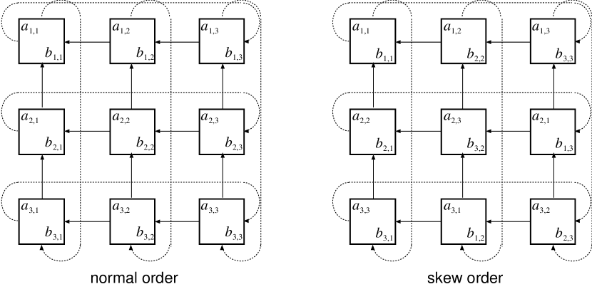
Figure 1: Preskewing of A and B.

The second systolic step of Cannon’s method consists of circular shifts of A along the rows and of B along the columns, followed by the computation event, cf. Fig. 2. We note that one can use blocks of elements as matrix entries.

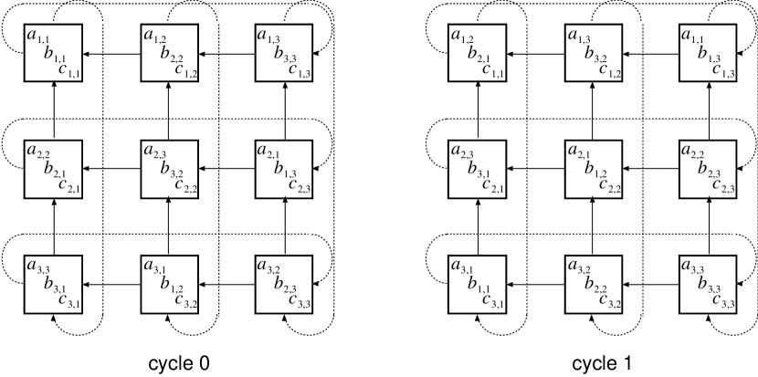
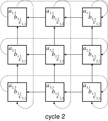
Figure 2: Systolic phase of Cannon’s algorithm.

The merit of Cannon’s algorithm lies in its memory efficiency, as it is possible to arrange the computation in such a way that no cell holds more than one element (block) of each matrix. Disadvantages of Cannon’s algorithm are pre-skewing and the fact that the optimal data layout for matrix multiplication requires one-to-all broadcast operations applied to matrix-vector multiplication. Furthermore the layout of the result vector differs from that of the input vector [27].

3 Design of a 1D Matrix Multiplication

In this section, we develop a 1D hyper-systolic matrix multiplication starting from a 2D algorithm that is related to the well known matrix product scheme of Fox [4]. In our systematic design approach the 2D scheme will be transformed to a 1D systolic array representation.

We have chosen a skew ordering as the fundamental representation of the matrices A, B and C. As a consequence, we will be able to carry out the computation fully in parallel without even the requirement for indexed addressing functionality of the target parallel computer. Furthermore, no reordering is required in the course of the computation because the skew representation is preserved.

3.1 Parallel Computational Problem

Given the $n\times m$ matrix A and the $m\times n$ matrix B, the matrix-matrix product reads

$$c_{i,j} = \sum_{k=1}^{m}a_{i,k}\,b_{k,j},\quad i,j=1,\dots,n.$$ (1)

On a distributed memory machine, the elements of A and B have to be spread appropriately across the different processor nodes.

In our design approach, we will first show how to multiply $4\times 4$ matrices A and B on a 2D grid of nodes of size $4\times 4$. Then, the algorithm is mapped onto a 1D processing array with $4$ nodes.

In Section 5, we present the hyper-systolic algorithm for matrix multiplication of $p\times p$ matrices on an array of $p$ processors.

In Section 6, we consider the general case Eq. 1 of multiplying a $n\times m$ matrix A and a $m\times n$ matrix B on a 1D system of $p$ processors. In order to map the systolic model onto a parallel implementation machine we choose hierarchy mapping with two different strategies, block and cyclic assignment.

3.2 2D Matrix Multiplication

3.2.1 Data alignment

In the following we make use of the concept of abstract processor arrays (APA) as defined in HPF [28].

The grid of boxes shown in Fig. 3 is such a 2D APA on which the matrices A, B and C involved in the operation $\mbox{\sf C}=\mbox{\sf A}\mbox{\sf B}$ are aligned in a column-skewed fashion.

Figure 3: Column-skewed distribution of the matrices A, B and C on a 2D APA.

3.2.2 Semi-systolic algorithm

Let the $p\times p$ matrices A, B and C be distributed on a $p\times p$ processor array and let for simplicity $p=4$.

The algorithm consists of $p$ (4) steps as follows: in the first step, the matrix elements $b_{1,1},b_{2,2},\dots,b_{p,p}$ of the matrix B in the first row of the APA are broadcast along the corresponding columns and subsequently are multiplied with the elements of the matrix A in the respective columns of the APA. The products (see Fig. 4a) are accumulated in the corresponding elements of the matrix C, according to the arrangement shown in Fig. 3.

At the end of the step, the elements of the matrix A are circularly shifted by one position to the left along the rows and by one position downwards along the columns (compare the positions of the elements of matrix A in Fig. 4a and Fig. 4b).

Figure 4: Computation of partial products on a 2D APA.

In the second step, the processors of the second row of the APA broadcast their corresponding elements of the matrix B in the respective columns of the APA, Fig.4b. This operation is followed by the same multiplication and accumulation operations and circular shifting of the elements of the matrix A as in the first step.

The algorithm proceeds with similar steps in which the processors of the third, through $p$-th row of the array broadcast in turn their elements of the matrix B, and the elements of matrix A are circularly shifted to the left and downwards by one position, cf. Fig.4c-d. After a total number of $p$ such steps all partial products which belong to the elements of the matrix C are accumulated in the corresponding processors.

The algorithm is called semi-systolic as it involves a broadcast operation of the row elements of B in each step.

3.2.3 Semi-hyper-systolic algorithm

We next consider the semi-hyper-systolic variant which corresponds to the semi-systolic algorithm just described. The initial distribution of data is shown in Fig. 5. The distribution of the matrices A and C is the same as the one shown in Fig. 3. The distribution of the matrix B is obtained from the distribution shown in Fig. 3 by circular shifting of the elements of B in the $i$-th row of the processor array by a stride of $(i-1){\,\mbox{{\footnotesize mod}}_{K}}$, with $K=2$ for $p=4$. In the particular example with $p=4$, the second and the fourth row of B are shifted by one position.

Figure 5: Initial distribution of data for the semi-hyper-systolic matrix product on a 2D APA.

The algorithm consists of $p$ (4) steps as shown in Fig. 6. In every step, each processor multiplies the elements of the matrix A with the elements of the matrix B which it receives via the associated broadcast line. The partial product thus computed is accumulated in one of two local variables. The local variables represent elements of two auxiliary arrays $\mbox{\sf C}^{(1)}$ and $\mbox{\sf C}^{(2)}$ which distributed across the processor array. They are used to accumulate partial results for the computations of the elements of the matrix C. Similar to the original systolic algorithm the processors in the first, second, …, $p$-th row broadcast the elements of the matrix B they contain to all the processors of the corresponding columns in the first, second, …, $p$-th step of the algorithm, respectively, see Fig. 6.

Figure 6: The products shown in the upper and the lower halves of the processors are accumulated in the auxiliary arrays $\mbox{\sf C}^{(1)}$ and $\mbox{\sf C}^{(2)}$.

At the end of each step the matrix A is cyclically shifted downwards by one position. Unlike the original algorithm the horizontal shift of the matrix A is performed only every second step by a stride of two elements.

The algorithm is completed by elemental addition of the auxiliary arrays $\mbox{\sf C}^{(1)}$ and $\mbox{\sf C}^{(2)}$ which is preceded by circular shifting of $\mbox{\sf C}^{(2)}$ by one position to the left.

3.2.4 Comparison to Cannon’s algorithm

The semi-hyper-systolic algorithm defined above can be compared with Cannon’s algorithm. Each of the two algorithms has merits and shortcomings: Cannon’s algorithm needs pre-skewing of the elements of the matrix A along the rows and the elements of matrix B along the columns of the 2D processor array which can be considered as a disadvantage since it gives rise to additional interprocessor communication that is not evenly distributed across the processors. On the other hand, the operations to be executed by each processor in a given step of the algorithm are rather simple, comprising one multiplication, one addition and two shift operations. Also, Cannon’s algorithm needs only local processor interconnections.

In contrast, the semi-hyper-systolic algorithm as illustrated in Fig. 6 needs broadcasting lines and more complex control of the operations which have to be carried out by the processors: in a given step, each processor has to broadcast an element to all other processors of the same column, and the matrix A is circularly shifted in two directions, where in horizontal direction a stride of $2$ is required for every second step while in vertical direction a stride of 1 is carried out in each step. On the other hand, this algorithm avoids pre-skewing of the matrices.

3.3 Matrix Multiplication on a 1D Processor Array

Next we transform the semi-systolic algorithm discussed above into a fully systolic one for a 1D processor array, in which a given processor executes in sequence the tasks assigned so far to the processors working on a given column of the 2D processor array. This procedure will eliminate the disadvantages of the semi-hyper-systolic 2D array algorithm since no broadcasting lines are needed, and moreover, control structures become simpler. Downward shifts of A merely amount to a re-assignment within the systolic cell and do not involve actual communication between cells. Note that the application of such a transformation on the algorithm of Cannon will not have the same effect as it would still be required to pre-skew one of the matrices.

3.3.1 Data alignment on a 1D processor array

In the case of a 1D processor array, we assign each column of the 2D array, Fig. 3, to one processor. The resulting layout of the matrices A, B and C is shown in Fig. 7. The dotted lines indicate the location of the elements in the cells of the previous 2D array.

Figure 7: APA with 1D systolic array alignment.

3.3.2 1D systolic algorithm

Again we start with the systolic computation. The algorithm needs $p$ (4) steps. It does not require a broadcast of the matrix elements of the matrix B. In the first step, the matrix elements $b_{1,1},b_{2,2},\dots,b_{p,p}$ of the matrix B which reside in the first, second, …, $p$-th processor, respectively, are multiplied with the elements of the respective columns of the matrix A. The products (see Fig. 8a) are accumulated in the corresponding elements of the matrix C, according to the arrangement shown in Fig. 7. At the end of the first step, the elements of the matrix A are circularly shifted by one position to the left along the rows.

Figure 8: APA for the systolic computation of partial products on a !D array.

In the second step, the second row of the matrix B is involved, see Fig. 8b. Its elements are multiplied by the elements of A and the partial products are accumulated in their proper locations, i. e., in the second step the products are copied to the elements of C which are circularly assigned one position downwards. Subsequently, A is circularly shifted to the left by one position.

The algorithm proceeds with similar steps in which the elements of the third, through $p$-th row the matrix B are multiplied with the elements of A, the products being assigned to a row of C at locations $i-1$ positions downwards the row in the $i$-th step, with the elements of matrix A being circularly shifted to the left, cf. Fig. 8c-d. After a total number of $p$ (4) steps all partial products which belong to the elements of the matrix C are accumulated in the corresponding processors.

3.3.3 1D hyper-systolic algorithm

Let us turn now to the 1D realization of the hyper-systolic algorithm. The initial distribution—as in the 2D case—requires a partial skewing of B along the rows, see Fig. 9. The distribution of the matrix B is obtained from the distribution shown in Fig. 7 by circular shifting of the elements of B in the $i$-th row of the processor array by a stride of $(i-1){\,\mbox{{\footnotesize mod}}_{K}}$, with $K=2$ for $p=4$.

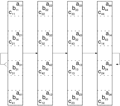
Figure 9: Initial distribution of data for the hyper-systolic matrix product on a 1D APA.

Step by step each processor multiplies the element of the matrix A it contains with the corresponding element of the matrix B. The partial product thus computed is accumulated in one of two local variables ($K=2$). The products computed in alternate steps are again stored alternately in one of the two local variables, in an analogous fashion as for the systolic algorithm, i. e., in the $i$-th step, the product is assigned to a row located $i-1$ elements downwards, cf. Fig. 10.

Figure 10: Hyper-systolic algorithm on a 1D array.

We emphasize again that A is shifted only every second step in horizontal direction to the left by two elements. For the general case with $p$ processors, we have to carry a shift by $\tilde{K}$ elements in every $K$-th step.

The algorithm is completed by elemental addition of the auxiliary arrays $\mbox{\sf C}^{(1)}$ and $\mbox{\sf C}^{(2)}$ which is preceded by circular shifting of $\mbox{\sf C}^{(2)}$ by one position to the left.

3.3.4 Summary

In a systematic design approach, we developed a matrix multiplication algorithm on a 1D abstract processor array, starting from an algorithm on a 2D APA. The algorithmic transformations led to a 1D hyper-systolic scheme

• that avoids broadcast lines required in the 2D case,

• that, given $p$ processors, shows a complexity of interprocessor communication on the 1D APA which is equal to that of Cannon’s 2D algorithm,

• that avoids skewing operations and reordering.

So far, we illustrated the scheme using $4\times 4$ matrices distributed column-wise over 4 systolic cells. In section 5, we generalize the $4\times 4$ problem to a $p\times p$ system, distributed on a $p$ processor array. In the case of the $4\times 4$ matrices, the shift constant was 2. For the general case, we shall introduce a stride $K$ which is carried out $\tilde{K}$ times, where the integer constants $K$ and $\tilde{K}$ fulfil $K\tilde{K}=p$.

4 Hyper-Systolic Bases

Before we present the general hyper-systolic matrix product, we define the hyper-systolic algorithm for two data streams. Such a situation is given in the computation of convolution and correlation problems. The scheme will later be adapted to the matrix multiplication [22].

4.1 Hyper-Systolic Recipe

Let x and z be two 1D arrays both of length $n$. Assume that functions

$$F_{i}=\bigoplus_{j=1}^{n}f(x_{i},z_{j})$$ (2)

for each $i$ have to be computed, with $\oplus$ being an associative and commutative operator. The computation can readily be carried out by usage of systolic algorithms on a ring of systolic cells [20]. However, one can observe redundant interprocessor communication in this process that can be removed in hyper-systolic processing. The general recipe to find optimal hyper-systolic bases reads:

Let the numerical problem be computable on two 1D systolic processor arrays by use of a 1D systolic algorithm. Let the two 1D data streams x and z both of length $n$ be mapped onto themselves by two sequences of (circular) shifts on the systolic array. The hyper-systolic scheme to compute the problem is constructed as follows:

1. For the systolic array x of length $n$, $k$ replicas are generated by shifting the array x $k$ times by strides $a_{t}$, $1\leq t\leq k$, where all shifted arrays are stored as intermediate elements on the cells as arrays $\hat{\mbox{\sf x}_{t}}$, $1\leq t\leq k$.

   For the systolic array z of length $n$, $k^{\prime}$ replicas are generated by shifting the array x $k^{\prime}$ times by strides $b_{t^{\prime}}$, $1\leq t^{\prime}\leq k^{\prime}$, where all shifted arrays are stored as intermediate elements on the cells as arrays $\hat{\mbox{\sf z}_{t^{\prime}}}$, $1\leq t^{\prime}\leq k^{\prime}$.

2. The sequences of strides $\{a_{t}\}$, $1\leq t\leq k$ and $\{b_{t^{\prime}}\}$, $1\leq t^{\prime}\leq k^{\prime}$ are determined such that

   1. all pairings of data elements are present at least once,

   2. the total communication cost is minimized.

3. After each communication event the computations can be carried out and the results are assigned to the corresponding intermediate result arrays $\hat{\mbox{\sf y}}_{t}$, $1\leq t\leq k+1$. If elements occur more than once they are accounted for by a multiplicity table in order to avoid multiple counting.

4. One collector array y is moved by strides that follow the inverse of the sequence $A_{k}$ of strides of the initial phase. In each step of the back-shift phase the required intermediate result arrays $\hat{\mbox{\sf y}}_{t}$ are added to y.

4.2 The Hyper-Systolic Optimization Problem

Parallel machines support logical 1D chains of processors in form of linear arrays or rings. However, circular shifts along the 1D ring in general lead to different hardware communication expenses for different strides.

The optimal sequence of strides for minimal interprocessor communication will depend on the interprocessor communication cost for a given stride. In order to minimize the communication cost effect on a given machine, we introduce a cost function ${C}(a_{i})$, as a function of the stride $a_{i}$.

For the sake of argumentation, let us first assume the costs of communication for each array x and z on the systolic ring to be constant for any stride $a_{i}$, $b_{i}$. $C(a_{i})=C(b_{\hat{i}})=\mbox{const}$.

Definition 1

- Optimization Problem for $C(a_{i})=C(b_{\hat{i}})=\mbox{const.}$
Let $I$ be the set of integers $m=\{0,1,2\dots,n-1\}\in{\mathbb{N}}^{n}_{0},n\in{\mathbb{N}}$. Find the two ordered multi-sets $A_{k}=(a_{0}=0,a_{1},a_{2},a_{3},\dots,a_{k})\in{\mathbb{N}}^{k+1}_{0}$ of $k+1$ integers and $B_{k^{\prime}}=(b_{0}=0,b_{1},b_{2},b_{3},\dots,b_{k^{\prime}})\in{\mathbb{N}}^{K+1}_{0}$ of $k^{\prime}+1$ integers, with $k+k^{\prime}$ being a minimum, where each $m\in I$, ($0\leq m\leq n-1$), can be represented at least once as the sum of two ordered partial sums

$$m=(a_{i}+a_{i+1}+\dots+a_{i+j})+(b_{\hat{i}}+b_{{\hat{i}}+1}+\dots+b_{{\hat{i}}+\hat{j}}),$$ (3)

with

$$0\leq i+j\leq k,\qquad i,j\in{\mathbb{N}}_{0},\qquad 0\leq\hat{i}+\hat{j}\leq k^{\prime},\qquad\hat{i},\hat{j}\in{\mathbb{N}}_{0}.$$ (4)

Lower bound on $k+k^{\prime}$

A lower bound for the minimal number of non-zero elements of $A_{k}$ can be derived that will deliver optimal complexity.

Theorem 1

Let $A_{k}$ and $B_{k^{\prime}}$ be two bases solving the optimization problem for the hyper-systolic algorithm with 2 arrays. Then the minimal length $k+k^{\prime}$ is given by

$$k=k^{\prime}=\sqrt{n}-1.$$ (5)

[Proof.] The total number of combinations required is $n^{2}$ as each element of the first array must come into contact with the $n$ elements of the second array. Let the matrices ${\cal H}_{1}$ and ${\cal H}_{2}$ be realized by $k-1$ and $k^{\prime}-1$ shifts respectively. In that case each element of the first matrix can be combined with $k^{\prime}$ elements of the second matrix, therefore the possible number of combinations will be $nkk^{\prime}$. Given $n=kk^{\prime}$, the minimum number of circular shifts $k+k^{\prime}$ is attained for $k=k^{\prime}=\sqrt{n}-1$. ∎

Therefore, the complexity for the interprocessor communication of a hyper-systolic algorithm for $C(a_{i})=C(b_{i})=\mbox{const.}$ is bounded from below by $3(\sqrt{n}-1)$ shifts, where we have already included the costs for the back-shifts.

4.3 ${C}(a_{i})$ and ${C}(b_{\hat{i}})\neq\mbox{const}$

We now assume that the cost for a circular shift is a function of the strides $a_{i}$. The optimization problem of definition 1 is modified only slightly, however, the construction of an optimal base can be quite complicated.

Definition 2

- Optimization Problem for $C(a_{i})=C(b_{\hat{i}})\neq\mbox{const.}$
Let $I$ be the set of integers $m=\{0,1,2\dots,n-1\}\in{\mathbb{N}}^{n}_{0},n\in{\mathbb{N}}$. Find the two ordered multi-sets $A_{k}=(a_{0}=0,a_{1},a_{2},a_{3},\dots,a_{k})\in{\mathbb{N}}^{k+1}_{0}$ of $k+1$ integers and $B_{k^{\prime}}=(b_{0}=0,b_{1},b_{2},b_{3},\dots,b_{k^{\prime}})\in{\mathbb{N}}^{K+1}_{0}$ of $k^{\prime}+1$ integers, with the total cost

$$C_{\mbox{\footnotesize total}}=\sum_{i=1}^{k}C(a_{i})+\sum_{\hat{i}=1}^{k^{\prime}}C(b_{\hat{i}})$$ (6)

being a minimum, where each $m\in I$, ($0\leq m\leq n-1$), can be represented at least once as the sum of two ordered partial sums

$$m=(a_{i}+a_{i+1}+\dots+a_{i+j})+(b_{\hat{i}}+b_{{\hat{i}}+1}+\dots+b_{{\hat{i}}+\hat{j}}),$$ (7)

with

$$0\leq i+j\leq k,\qquad i,j\in{\mathbb{N}}_{0},\qquad\hat{i}+\hat{j}\leq k^{\prime},\qquad\hat{i},\hat{j}\in{\mathbb{N}}_{0}.$$ (8)

4.4 Regular Bases

The $4\times 4$ problem presented in Section 3 uses so-called regular bases. This prescription turns out to be optimal for equal cost of any stride executed in circular shift operations on the ring. Regular hyper-systolic bases are advantageous as they require only two distinct strides.

Definition 3

- Regular Bases The regular bases are given by

$$\begin{array}[]{ccccccccc}A_{k=K-1}&:=&\Big{(}0,&1,1,\dots,1\Big{)}\\ &&&\underbrace{\makebox[34.14322pt]{}}&\\ &&&K-1\\ \end{array},\quad\begin{array}[]{ccccccccc}B_{k^{\prime}=\tilde{K}-1}&:=&\Big{(}0,&K,K,\dots,K\Big{)}\\ &&&\underbrace{\makebox[45.52458pt]{}}&\\ &&&\tilde{K}-1\\ \end{array},\quad K\times\tilde{K}=n.$$ (9)

The completeness of a base pair is defined in terms of the $h$-range of the base, a notion borrowed from additive number theory [29, 30]:

Theorem 2

The $h$-range of a regular base is $n$.

[Proof.] Let

$$r:=m{\,\mbox{{\footnotesize mod}}_{\tilde{K}}}\rightarrow r<K,$$ (10)

as $K\tilde{K}=n$. There are $K-1$ elements $a_{i}=1\in A_{k}$. Thus any $r$ with $0\leq r\leq K-1$ $r\in{\mathbb{N}}_{0}$ can be represented as partial sum by the elements $a_{i}=1$, $a_{i}\in A_{k}$. The partial sums of $B_{k^{\prime}}$,

$$\sum_{l=i}^{j}b_{l}=K\sum_{l=i}^{j}1=(j-i+1)K<n,$$ (11)

are integer multiples of K. Adding the partial sums to $r$ we can therefore represent any element $m\in I$. Thus, the $h$-range of the base pair $A_{k=K-1}$ and $B_{k^{\prime}=\tilde{K}-1}$ is $n$, i. e., the base pair is complete. ∎

Theorem 3

The lower bound to the minimal length of the regular bases for a given $h$-range $n$ is $K=\tilde{K}=\sqrt{n}$.

[Proof.] The regular base $A_{k}$ is complete.

$$k=K+\tilde{K}-1\rightarrow k=K+\frac{n}{K}-1.$$ (12)

Differentiation gives $K=\sqrt{n}$. ∎

Theorem 4

The communication gain factor $R$ that compares the regular hyper-systolic to the systolic algorithm is:

$$R=\frac{n-1}{2K+\tilde{K}-3}\approx\frac{\sqrt{n}}{3}.$$ (13)

[Proof.] Let $K=\tilde{K}=\sqrt{n}$. One needs $K-1$ shifts by $1$ and $\tilde{K}-1$ shifts by $K$ in forward direction and again $K-1$ shifts by $1$ in backward direction, respectively; therefore, the total number of shifts required turns out to be

$$T=(2K+\tilde{K}-3).$$ (14)

The standard systolic computation requires $n-1$ shifts altogether. ∎

5 Hyper-Systolic Matrix Product

Next we present the general formulation of the systolic and hyper-systolic matrix product in terms of a pseudo-code formulation. The size of the matrices is $p\times p$ and the 1D processor array consists of $p$ nodes.

5.1 Systolic Algorithm

The systolic version of the matrix product of two matrices A and B is given in Algorithm 1. The matrices are represented in skew order.

Algorithm 1

Systolic matrix-matrix multiplication.

foreach processor $i=1:p$ $\in$ systolic array
	for $j=1:p$
		for $l=1:p$
			$c_{l,i}=c_{l,i}+\mbox{{\sf cshift-col}}_{p}^{1-j}(a_{l,i})\,b_{j,i}$
		end for
		for $k=1:p$
			$a_{k,i}=\mbox{{\sf cshift-row}}_{p}^{1}(a_{k,i})$
		end for
	end for
end foreach

We have simplified the representation of data movements and assignments by introduction of two functions:

cshift-row: horizontal circular shift of data by a stride of $k$ on a ring of cells numbered from $1$ to $n$, cshift-row involves interprocessor communication.

$$\mbox{{\sf cshift-row}}_{n}^{k}(a_{j,i}):=a_{j,(i+k-1+n){\,\mbox{{\footnotesize mod}}_{n}}+1}.$$ (15)

cshift-col: vertical circular shift by a stride of $k$ for the vector of $n$ elements within the systolic cells. cshift-col only amounts to memory assignments.

$$\mbox{{\sf cshift-col}}_{n}^{k}(a_{j,i}):=a_{(j+k-1+n){\,\mbox{{\footnotesize mod}}_{n}}+1,i}.$$ (16)

The algorithm is completely regular. Each cell executes one compute operation together with an assignment followed by a circular shift of the matrix A in each systolic cycle. The skew order is not destroyed during execution of the algorithm. Note that for each processor inner cell assignment operations (col-cshift) are executed using equal strides in a given step of the parallel algorithm. Hence, one global address suffices and further address computations are not required!

5.2 Hyper-systolic Algorithm

It has been already noticed in section 3.3, that the complexity of the systolic computation is not competitive with Cannon’s algorithm. However, the hyper-systolic computation belongs to the same complexity class as Cannon’s algorithm. It is fully pipelined and parallel, and does not require any skewing steps to align or re-align matrix elements.

5.2.1 Regular Bases

We employ the regular bases constructed for the hyper-systolic system. We add a third base $C$ to account for the back shifts:

$$\begin{array}[]{rrrrrrrrrrrrrrrrrrrr}A_{k=\tilde{K}-1}&=\Big{(}&0,&K,&K,&\dots,K&\Big{)}\\ B_{k^{\prime}=K-1}&=\Big{(}&0,&-1,&-1,&\dots,-1&\Big{)}\\ C_{k^{\prime}=K-1}&=\Big{(}&0,&1,&1,&\dots,1&\Big{)}\\ \end{array}\,.$$ (17)

5.2.2 Hyper-systolic matrix multiplication

The hyper-systolic matrix multiplication, as given in Algorithm 2, proceeds within three steps. In the first part of the algorithm, matrix B is shifted $K-1$ times by strides of $1$ along the systolic ring and stored as $B^{i}$, $0\leq i\leq K-1$. However, as motivated above, for the case of matrix products, we can spare communication: it suffices to shift B in $\tilde{K}$ row blocks of $K$ rows each, where within each block the first row is shifted by a stride of $0$ and the last by a stride of $K-1$.

Algorithm 2

Hyper-systolic matrix multiplication.

foreach processor $i=1:p$ $\in$ systolic array
	for $j=1:p$				! pre-shift of matrix B
		$b_{j,i}=\mbox{{\sf cshift-row}}_{p}^{[(1-j){\,\mbox{{\footnotesize mod}}_{K}}]}\big{(}b_{j,i}\big{)}$
	end for
	for $j=1:\tilde{K}-1$				! multiplication and shift of matrix A
		for $l=1:K$
			for $n=1:p$
				$c^{l}_{n,i}=c^{l}_{n,i}+\mbox{{\sf cshift-col}}_{p}^{[1-(j-1)K-l]}\big{(}a_{n,i}\big{)}\,b_{[(j-1)K+l],i}$
			end for
		end for
		for $l=1:p$
			$a_{l,i}=\mbox{{\sf cshift-row}}_{p}^{K}\big{(}a_{l,i}\big{)}$
		end for
	end for
	for $l=1:K$
		for $n=1:p$
			$c^{l}_{n,i}=c^{l}_{n,i}+\mbox{{\sf cshift-col}}_{p}^{[1-(\tilde{K}-1)K-l]}\big{(}a_{n,i}\big{)}\,b_{[(\tilde{K}-1)K+l],i}$
		end for
	end for
	for $j=1:K-1$				! back shift and accumulation
		for $l=1:p$
			$c^{K-j}_{l,i}=c^{K-j}_{l,i}+\mbox{{\sf cshift-row}}_{p}^{1}\big{(}c^{K-j+1}_{l,i}\big{)}$
		end for
	end for
end foreach

After the preparatory shifts of B, the computation starts. $\tilde{K}$ times, the multiplication of A with $K$ rows of the pre-shifted matrix B is carried out. After each step, A is moved to the left by a shift of stride $K$. The result is accumulated within $K$ matrices $\mbox{\sf C}^{i}$.

Finally, the $K$ intermediate result matrices $\mbox{\sf C}^{i}$ are shifted back according to base $C_{k^{\prime}}$ while summed up to the final matrix C. The algorithm is very regular. The skew order is not destroyed during execution, and in any stage, only global addresses are required.

5.2.3 Complexity

The gain factor for the matrix product reads (note that matrix B is only partially shifted):

Theorem 5

The gain factor $R$ that compares the regular hyper-systolic matrix multiplication to the systolic algorithm is

$$R=\frac{p-1}{K+\tilde{K}-1}\approx\frac{\sqrt{p}}{2}.$$ (18)

[Proof.] One needs $1$ shift of the full matrix B, $\tilde{K}-1$ shifts by $K$ of matrix A and again $K-1$ shifts by $1$ of matrix C. Therefore, the total number of shifts required is

$$T=(K+\tilde{K}-1).$$ (19)

The standard systolic computation requires $p-1$ shifts of the matrix A. For the $K=\tilde{K}=\sqrt{p}$, $R\approx\frac{\sqrt{p}}{2}$. ∎

5.2.4 Comparison to Cannon’s algorithm

In order to compare Cannon’s algorithm and the hyper-systolic matrix multiplication, we consider a 2D $\sqrt{p}\times\sqrt{p}$ processor array, where Cannon’s algorithm is carried out, and a 1D ring array of $p$ processors where the hyper-systolic matrix product algorithm is computed.

The total number of shift operations of Cannon’s algorithm is $2\sqrt{p}-2=2K-2$, while the number of shift operations for the hyper-systolic algorithm was $2K-1$. Thus, the complexities in terms of circular shift operations of both algorithms are equal for large $p$. We will see below how this fact translates into execution times on mesh and grid based machines.

6 Mapping on Parallel Systems

So far we discussed the generic situation of the matrix dimension $p$ being equal to the number of processors $p$. We now turn to the general case of square $n\times m$-matrices with $n,m>p$.

In order to map the systolic system onto the parallel implementation machine we choose hierarchy mapping of the systolic array onto the processors with the option for two different strategies, block and cyclic assignment.

6.1 Block Mapping

The block assignment is applied in all standard algorithms, as it allows to exploit local BLAS-3 routines, like dgemm, by which a very high efficiency of local computations can be achieved. While a small block of the matrix A is hold in the cache or in the registers (thus avoiding cache-to-memory data transfer), in turn, only the columns of B and C must be exchanged, and all computations in which the given part of A is involved can be carried out. In this way, the ratio between the number of computations and the cache-to-memory traffic is minimized to nearly

$$\frac{2l^{3}}{(3nn+n^{2})}=\frac{l}{2}$$ (20)

floating point operations per word for real data, with $l$ being the dimension of the sub-block. Asymptotically, the full speed of the CPU should be exploitable.

A $n\times m$-matrix M is divided into $p\times p$ blocks of size $\left(\frac{n}{p}\times\frac{m}{p}\right)$ or $\left(\frac{m}{p}\times\frac{n}{p}\right)$,

$$\mbox{\bf M}\rightarrow\mbox{\sf M}_{i,j},\quad i=1,\dots,p,\quad j=1,\dots,p.$$ (21)

The multiplication of A and B proceeds via sub-matrix multiplication denoted as $(\otimes)$:

$$\mbox{\sf C}_{i,j} = \sum_{k=1}^{p}\mbox{\sf A}_{i,k}\otimes\mbox{\sf B}_{k,j},\quad i=1,\dots,p,\quad j=1,\dots,p,$$

C $$= \mbox{\bf A}\mbox{\bf B}.$$ (22)

Altogether a system of $p\times p$ of such blocks is assigned to the $p$ processor array. Now we can use each sub-matrix in the same manner as the scalar matrix elements before. Therefore, the $p\times p$ system of sub-matrices has to be row-skewed for A and column-skewed for B.

6.2 Cyclic Mapping

Each block is distributed across the processors as described above for the generic case. The blocking of the $n\times m$-matrix M into $\left(\frac{n}{p}\times\frac{m}{p}\right)$ blocks, leads to blocks of size $p\times p$,

$$\mbox{\bf M}\rightarrow\mbox{\sf M}_{i,j},\qquad i=1,\dots,\frac{n}{p},\;j=1,\dots,\frac{m}{p}.$$ (23)

The multiplication of A and B proceeds via block-multiplication, $(\otimes)$:

$$\mbox{\sf C}_{i,j} = \sum_{k=1}^{\frac{m}{p}}\mbox{\sf A}_{i,k}\otimes\mbox{\sf B}_{k,j},\qquad i=1,\dots,\frac{n}{p},\quad j=1,\dots,\frac{n}{p},$$

C $$= \mbox{\bf A}\mbox{\bf B}.$$ (24)

A skew representation is required for all blocks $\mbox{\sf M}_{i,k}$ separately. Cyclic mapping leads to a system of $\frac{n}{p}\times\frac{m}{p}$ systolic processes that run in parallel.

Cyclic assignment allows us to reduce the memory overhead of hyper-systolic computations. In general, $K$ full intermediate matrices C are necessary. Using cyclic mapping, one can organize the computation in such a way that only one row of the blocks of the intermediate matrix C must be stored in a given phase of the algorithm. All the required shifts of the given part of A can be carried out while this part of A will not be involved in a further computation. Eventually, the corresponding row of C is shifted back and accumulated.

A second interesting feature of cyclic mapping is the possibility to distribute the very blocks. This approach is interesting for machines with a hybrid architecture like the proposed Italian PQE2000 system [31]. In this approach, the rows of A and the columns of B are assigned to different processors each.

6.3 Block-Cyclic Mapping

One can combine block and cyclic mapping in a hybrid scheme that combines the advantages of both approaches. A good strategy is to choose the block size of the block mapping such that it is optimal for “local” BLAS-3. For the cyclic part one ends up with blocks of size $p\times p$, with the entries being the BLAS-3 blocks.

7 Implementation Issues

The class of algorithm presented can be useful on any type of massively parallel system with distributed memory. Mesh and grid-based connectivities might benefit as well as large work-station clusters.

In the previous section, we have presented complexities of interprocessor communication in terms of circular shifts, irrespective of the actual communication time of a shift. This time is a constant on workstation clusters usually connected via Ethernet, therefore complexities in terms of circular shifts will translate into real time in a straightforward way. On mesh and grid based machines 1D rings in general can be realized as a subset of their system connectivity.

Figure 11: Performance of systolic and hyper-systolic PBLAS-3 (block-cyclic mapping) on a 128-node APE100, for real and complex data.

As an example taken from real life, we have implemented a level-3 PBLAS code on the APE100 parallel computer. So far, on APE100 lack of indexed addressing has hindered an effective scalable implementation of PBLAS [32]. In our approach, we made use of a combination of block and cyclic mapping. Thus, we are able to use local BLAS, exploiting the CPU with high efficiency, and to reduce the memory overhead of the hyper-systolic algorithm.

On APE100, for real data, the optimal elementary blocks are of size $6\times 6$. For complex data, the size is $4\times 4$. The full matrix is blocked to $p\times p$ matrices which are distributed on the ring and the elements of which are the elementary blocks. Only the $p\times p$ matrices are skew, the elementary matrices remain in normal order.

We have benchmarked a 128-node APE/100Quadrics QH1 using real and complex data. Fig. 11 shows the performance results.

The theoretical peak performances (single node!) for Quadrics are $63$ % for real data and $88$ % for complex data, as can be inferred from the maximal ratio of computation vs. memory-to-register data transfer times. Hyper-systolic matrix multiplication leads to a peak performance of 65 % of peak speed, which translates into 75 % of the theoretical performance.

8 Summary

The 1D hyper-systolic matrix multiplication algorithm is a promising alternative to 2D matrix product algorithms. With equal complexity as standard methods, the hyper-systolic algorithm avoids non-regular communication and indexed local addressing. Hence, the hyper-systolic matrix product scheme is universal: it is applicable on any type of parallel system, even on machines that cannot compute local addresses. The method preserves the alignment of the matrices in the course of the computation. Besides the fact that transposed matrix products can be carried out on the same footing, alignments for the optimal hyper-systolic algorithm are efficient for matrix-vector operations as well.

So far, in a feasibility study, the hyper-systolic matrix product has been implemented on APE100/Quadrics systems [33, 34]. We will present details of the implementation on this system for matrix and transposed matrix products in Ref. [35].

References

- [1] J. Choi, J. J. Dongarra, and D. W. Walker: “The Design of Scalable Software Libraries for Distributed Memory Concurrent Computers”, in: J. J. Dongarra and B. Tourancheau (eds.): Environments and Tools for Parallel Scientific Computing (Elsevier, 1992).
- [2] Th. Lippert, A. Seyfried, A. Bode, K. Schilling: ‘Hyper-Systolic Parallel Computing’, IEEE Trans. on Parallel and Distributed Systems 9 (1998) 1.
- [3] A. Galli: ‘Generalized Hyper-Systolic Parallel Computing’, preprint server hep/lat, URL: http://xxx.lanl.gov/ps/hep-lat/9509011
- [4] G. C. Fox and S. W. Otto: ‘Matrix Algorithms on a Hypper-Cube I: Matrix Multiplication’, Parallel Computing 4 (1987) 17-31.
- [5] N. Petkov: Systolische Algorithmen und Arrays (Berlin: Akademie-Verlag, 1989).
- [6] N. Petkov: Systolic Parallel Processing (Amsterdam: North-Holland, 1993).
- [7] H.T. Kung and C. E. Leiserson: “Systolic arrays (for VLSI)”, Sparse Matrix Proc. 1978 (Society for Industrial and Applied Mathematics, 1979) pp.256-282; the same as “Algorithms for VLSI processor arrays”, in C. Mead and L. Conway: Introduction to VLSI Systems (Reading, MA: Addison-Wesley, 1980) sect.8.3.
- [8] H.T. Kung: “Why systolic architectures”, Computer 15 (1981) pp.37-47.
- [9] P.R. Cappello and K. Steiglitz: “Unifying VLSI design with geometric transformations”, Proc. Int. Conf. Parallel Processing (1983) 448-457.
- [10] P.R. Cappello: “Space time transformation of cellular algorithms”, in E.E. Swartzlander (ed.), Systolic Signal Processing Systems (N.Y., Basel: Dekker, 1987), 161-208.
- [11] P. Quinton: “Automatic synthesis of systolic arrays from uniform recurrent equations”, Proc. 11th Annual Int. Symp. Comput. Archit., Ann Arbor, Mich., 1984 (IEEE, N.Y., 1984) pp. 208-214.
- [12] D.I. Moldovan: ”On the analysis and synthesis of VLSI algorithms”, IEEE Trans. on Computers C-31 (1982) 1121-1126.
- [13] D.I. Moldovan: “On the design of algorithms for VLSI systolic arrays”, Proc. IEEE 71 (1983) 113-120.
- [14] P. Clauss, G. R. Perrin: “Optimal Mapping of Systolic Algorithms by Regular Instruction Shifts”, IEEE International Conference on Application-Specific Array Processors, ASAP (1994) 224-235.
- [15] A. Darte, Y. Robert: “Affine-by-Statement scheduling of uniform and affine loop nests over parametric domains”, Journal of Parallel and Distributed Computing, 29 (1995) 43-59.
- [16] P. Clauss , V. Loechner, “Parametric analysis of polyhedral iteration spaces”, IEEE International conference on Application Specific Array Processors, ASAP, 1996.
- [17] T. Dontje, Th. Lippert, N. Petkov and K. Schilling: “Statistical analysis of simulation-generated time series: Systolic vs. semi-systolic correlation on the Connection Machine”, Parallel Computing 18 (1992) 575-588.
- [18] N. Petkov: ‘Fuzzy number subtraction convolution on the CM-2’, Int. J. of Mod. Phys. C4 (1993) 181-196.
- [19] N. Petkov: ‘Fuzzy number subtraction convolution on the CM-2’, in: Th. Lippert, K. Schilling and P. Ueberholz (eds.) Science on the Connection Machine (Singapore: World Scientific, 1993), pp. 181-196.
- [20] Th. Lippert, U. Glaessner, H. Hoeber, G. Ritzenhöfer, K. Schilling, and A. Seyfried: ‘Hyper-Systolic Processing on APE100/Quadrics, I. -loop computations’, Int. Jour. Mod. Phys. C 7 (1996) 485.
- [21] G. Meylan and D. C. Heggie: ‘Internal Dynamics of Globular Clusters’, preprint HEP-ASTRO, http://xxx.lanl.gov/multi, in press in The Astronomy and Astrophysics Review.
- [22] Th. Lippert: ‘Hyper-Systolic Parallel Computing—Theory and Applications’, PhD-thesis, University of Groningen, 1998.
- [23] J. O. Eklundth: ‘A fast Computer Method for Matrix Transposing’, IEEE Trans. on Computers C 21 (1972) 801-803.
- [24] F. DePrez and M. Pourzandi: ‘A Comparison of three Parallel Matrix Product Algorithms’, Proc. of the Int. Conf. Advances in Numerical Methods & Applications, Sofia (1994) 234-244.
- [25] H. Gupta and P. Sadayappan: ‘Communication Efficient Matrix Multiplication on Hypercubes’, Parallel Computing 22 (1996) 75-99.
- [26] L. E. Cannon: ‘A Cellular Computer to Implement the Kalman Filter Algorithm’, PhD Thesis, Montana State University, 1969.
- [27] V. Kumar, A. Grama, A. Gupta, and G. Karypis: Introduction to Parallel Computing (Redwood City: Benjamin/Cummings, 1994).
- [28] ‘High Performance Fortran Language Specification,’ Rice University, version 1.1 November 1994. ‘High Performance Fortran’, Scientific Programming, 2 (1993).
- [29] M. Djawadi and G. Hofmeister: ‘The Postage Stamp Problem’, Mainzer Seminarberichte, Additive Zahlentheorie 3 (1993) 187.
- [30] R. K. Guy, Unsolved Problems in Number Theory, (Springer-Verlag, Berlin, New-York, 1994).
- [31] URL:(http://www.sede.enea.it/ hpcn/moshpce/hpcn01e.html)
- [32] M. Beccaria, G. Cella, A. Ciampa, G. Curci, and A. Viceré: ‘Matrix Inversion on APE100 Machines’, Preprint IFUP-TH 17/95.
- [33] Th. Lippert and K. Schilling: ‘Hyper-Systolic Matrix Multiplication’, in: H. R. Arabnia (ed.), Proceedings of the International Conference on Parallel and Distributed Processing Techniques and Applications, PDPTA ’96, Sunnyvale, California, USA, - August 9 - 11, 1996, (CSREA, 1996), pp. 919-930.
- [34] Th. Lippert, N. Petkov, and K. Schilling: ‘BLAS-3 for the Quadrics Parallel Computer’, in: B,. Hertzberger and P. Sloot (eds.), Proceedings of the International Conference on High Performance Computing and Networking, HPCN ’97, Vienna, Austria, April 1997, (Springer, Berlin, 1997) pp. 332-341. 919-930.
- [35] M. Coletta, Th. Lippert, P.Palazzari, N. Petkov, and K. Schilling: to appear.