Approximation Algorithms for PSPACE-Hard Hierarchically and Periodically Specified Problems

Abstract

We study the efficient approximability of basic graph and logic problems in the literature when instances are specified hierarchically as in [35] or are specified by 1-dimensional finite narrow periodic specifications as in [58]. We show that, for most of the problems $\Pi$ considered when specified using k-level-restricted hierarchical specifications or $k$-narrow periodic specifications, the following holds:

1. Let $\rho$ be any performance guarantee of a polynomial time approximation algorithm for $\Pi$, when instances are specified using standard specifications. Then $\forall\epsilon>0$, $\Pi$ has a polynomial time approximation algorithm with performance guarantee $(1+\epsilon)\rho$.

2. $\Pi$ has a polynomial time approximation scheme when restricted to planar instances.

These are the first polynomial time approximation schemes for PSPACE-hard hierarchically or periodically specified problems. Since several of the problems considered are PSPACE-hard, our results provide the first examples of natural PSPACE-hard optimization problems that have polynomial time approximation schemes. This answers an open question in Condon et. al. [8].

1 Introduction and motivation

Many practical applications of graph theory and combinatorial optimization in CAD systems, mechanical engineering, VLSI design and software engineering involve processing large objects constructed in a systematic manner from smaller and more manageable components. An important example of this occurs in VLSI technology. Currently, VLSI circuits can consist of millions of transistors. But such large circuits usually have a highly regular design and consequently are defined systematically, in terms of smaller circuits. As a result, the graphs that abstract the structure and operation of the underlying circuits (designs) also have a regular structure and are defined systematically in terms of smaller graphs. Methods for describing large but regular objects by small descriptions are referred to as succinct specifications. Over the last twenty years several theoretical models have been put forward to succinctly represent objects such as graphs and circuits. (see for example [5, 6, 11, 19, 23, 26, 27, 34, 48, 50, 57]). Here, we study two kinds of succinct specifications, namely, hierarchical and periodic specifications.

Hierarchical specifications allow the overall design of an object to be partitioned into the design of a collection of modules; which is a much more manageable task than producing a complete design in one step. Such a top down (or hierarchical design) approach also facilitates the development of computer aided design (CAD) systems, since low-level objects can be incorporated into libraries and can thus be made available as submodules to designers of large scale objects. Other areas where hierarchical specifications have found applications are VLSI design and layout [18, 19, 55], finite element analysis, software engineering and datalog queries (see [18, 43] and the references therein). Periodic specifications can also be used to define large scale systems with highly regular structures. Using periodic specifications, large objects are described as repetitive connections of a basic module. Frequently, the modules are connected in a linear fashion, but the basic modules can also be repeated in two or higher dimensional patterns. Periodic specifications are also used to model time variant problems, where the constraints or demands for any one period is the same as those for preceding or succeeding periods. Periodic specifications have applications in such diverse areas as transportation planning [18, 43, 48], parallel programming [18, 26] and VLSI design [23, 24].

Typically, the kinds of hierarchical and periodic specifications studied in the literature are generalizations of standard specifications used to describe objects. An important feature of both these kinds of specifications is that they can be much more concise in describing objects than standard specifications. In particular, the size of an object can be exponential in the size of its periodic or hierarchical specifications. As a result of this, problems for hierarchically and periodically specified inputs often become PSPACE-hard, NEXPTIME-hard, etc.

In this paper, we concentrate our attention on

1. the hierarchical specifications of Lengauer [31, 34, 35] (referred to as L-specifications) and

2. the 1-dimensional finite periodic specifications of Gale and Wanke [10, 58] (referred to as 1-FPN-specifications).

Both of these specifications have been used to model problems in areas such as CAD systems and VLSI design [35, 32, 36], transportation planning [10], parallel programming [58], etc. We give formal definitions of these specifications in §4 and §5.

Let $\Pi$ be a problem posed for instances specified using standard specifications. For example, if $\Pi$ is a satisfiability problem for CNF formulas, the standard specification is sets of clauses, with each clause being a set of literals. Similarly if $\Pi$ is a graph problem, the adjacency matrix representation or the adjacency list representation of the edges in the graph are standard specifications. For the rest of the paper, we use

1. l-$\Pi$ to denote the problem $\Pi$, when instances are specified using the hierarchical specifications of Lengauer [35] (see Definition 1), and

2. 1-fpn-$\Pi$ to denote the problem $\Pi$, when instances are specified using the 1-dimensional finite periodic specifications of Wanke [58] (see Definition 5).

Thus for example, l-3sat denotes the problem 3sat when instances are specified using L-specifications and 1-fpn-3sat denotes the problem 3sat when instances are specified using 1-FPN-specifications. For the rest of this paper, we use the term succinct specifications to mean both L-specifications and 1-FPN-specifications.

2 Summary of results

In this paper, we discuss a natural syntactic restriction on the L-specifications and call the resulting specifications level-restricted specifications. (For 1-FPN-specifications our notion of level-restricted specifications closely coincides with Orlin’s notion of narrow specifications [48].) Most of the problems considered in this paper are PSPACE-hard even for level-restricted specifications (see [37, 44, 48]). Consequently, we focus our attention on devising polynomial time approximation algorithms for level restricted L- or 1-FPN-specified problems. Recall that an approximation algorithm for a minimization problem $\Pi$ provides a performance guarantee of $\rho$ if for every instance $I$ of $\Pi$, the solution value returned by the approximation algorithm is within a factor $\rho$ of the optimal value for $I$. A polynomial time approximation scheme (PTAS) for problem $\Pi$ is a family of algorithms such that, for $\epsilon>0$, given an instance $I$ of $\Pi$, there is a polynomial time algorithm in the family that returns a solution which is within a factor $(1+\epsilon)$ of the optimal value for $I$. The main contributions of this paper include the following.

1. We design polynomial time approximation algorithms (for arbitrary instances ) and approximation schemes (for planar instances) for a variety of natural PSPACE-hard problems specified using level-restricted L- or 1-FPN-specifications. These are the first polynomial time approximation schemes in the literature for “hard” problems specified using either L- or 1-FPN-specifications.To obtain our results we devise a new technique called the partial expansion. The technique has two desirable features. First, it works for a large class of problems and second, it works well for both L-specified and 1-FPN-specified problems.

2. For problems specified using level-restricted L- or 1-FPN-specifications, we devise polynomial time approximation algorithms with performance guarantees that are asymptotically equal to the best possible performance guarantees for the corresponding problems specified using standard specifications.

3. The results presented in this paper are a step towards finding sufficient syntactic restrictions on the L- or 1-FPN-specifications that allow us to specify a number of realistic designs in a succinct manner while making them amenable for rapid processing.

Our results provide the first examples of natural PSPACE-complete problems whose optimization versions have polynomial time approximation schemes. Thus they affirmatively answer the question posed by Condon, Feigenbaum, Lund and Shor [8] of whether there exist natural classes of PSPACE-hard optimization problems that have polynomial time approximation schemes.

2.1 The meaning of approximation algorithms for succinctly specified problems

When objects are represented using L- or 1-FPN-specifications, there are several possible ways of defining what it means to “design a polynomial time approximation algorithm”. Corresponding to each decision problem $\Pi$, specified using either L- or 1-FPN-specifications, we consider four variants of the corresponding optimization problem. We illustrate this with an example.

Example 1: Consider the minimum vertex cover problem, where the input is an L-specification of a graph $G$. We provide efficient algorithms for the following versions of the problem.

1. The construction problem: Output an L-specification of the set of vertices in the approximate vertex cover $\mathcal{C}$.

2. The size problem: Compute the size of the approximate vertex cover $\mathcal{C}$ for $G$.

3. The query problem: Given any vertex $v$ of $G$ and the path from the root to the node in the hierarchy tree (see §2 for the definition of hierarchy tree) in which $v$ occurs, determine whether $v$ belongs to the vertex cover $\mathcal{C}$.

4. The output problem: Output the approximate vertex cover $\mathcal{C}$.

Note that our algorithms for the four variants of the problem apply to the same vertex cover $\mathcal{C}$. Our algorithms for (1), (2) and (3) above run in time polynomial in the size of the L-specification rather than the size of the graph obtained by expanding the L-specification. Our algorithm for (4) runs in time linear in the size of the expanded graph but uses space which is only polynomial in the size of the L-specification. $\Box$

Analogous variants of approximation algorithms can be defined for problems specified using 1-FPN-specifications. Therefore, we omit this discussion.

These variants are natural extensions of the definition of approximation algorithms for problems specified using standard specifications. This can be seen as follows: When instances are specified using standard specifications, the number of vertices is polynomial in the size of the description. Given this, any polynomial time algorithm to determine if a vertex $v$ of $G$ is in the approximate minimum vertex cover can be easily modified to obtain a polynomial time algorithm that lists all the vertices of $G$ in the approximate minimum vertex cover. Thus in the case when inputs are specified using standard specifications, (3) can be used to solve (2) and (4) in polynomial time. The above discussion also shows that given an optimization problem specified using standard specifications, variants (1), (3) and (4) discussed above are polynomial time inter-reducible.

The approximation algorithms given in this paper have another desirable feature. For an optimization problem or a query problem, our algorithms use space and time which is a low level polynomial in the size of the hierarchical or the periodic specification. This implies that for graphs of size $N$, that are specified using specifications of size $O(polylog\,N)$, the time and space required to solve problems is only $O(polylog\,N)$. Moreover when we need to output the subset of vertices, subset of edges, etc. corresponding to a vertex cover, maximum cut, etc., in the expanded graph, our algorithms take essentially the same time but substantially less (often logarithmically less) space than algorithms that work directly on the expanded graph. The graphs obtained by expanding hierarchical or periodic descriptions are frequently too large to fit into the main memory of a computer [31]. This is another reason for designing algorithms which exploit the regular structure of the underlying graphs. Indeed, most of the standard algorithms in the literature assume that the input completely resides in the main memory. As a result, even the most efficient algorithms incur a large number of page faults while executing on the graphs obtained by expanding the hierarchical or periodic specifications. Hence, algorithms designed for solving problems for graphs or circuits represented in a standard fashion are often impractical for succinctly specified graphs. We refer the reader to [31, 36] for more details on this topic.

The rest of the paper is organized as follows. Section 3 contains discussion of related research. In §4, §5 and §6 we give the basic definitions and preliminaries. In §7 we discuss our approximation algorithms for L-specified problems and 1-FPN-specified problems. Finally in §8, we give concluding remarks and directions for future research.

3 Related research

In the past, much work has been done on characterizing the complexity of various problems when instances are specified using L- or 1-FPN-specifications. For periodically specified graphs, several researchers [6, 7, 19, 26, 27, 49, 50] have given efficient algorithms for solving problems such as determining strongly connected components, testing for existence of cycles, finding minimum cost paths between a pair of vertices, bipartiteness, planarity and minimum cost spanning forests. Orlin [50] and Wanke [58] discuss NP- and PSPACE-hardness results for infinite and finite periodically specified graphs.

For L-specified graphs, Lengauer et al. [32, 34, 35] and Williams et al. [59] have given efficient algorithms to solve several graph theoretic problems including 2-coloring, minimum spanning forests and planarity testing. Lengauer and Wagner [37] show that the following problems are PSPACE-hard when graphs are L-specified: 3 coloring, Hamiltonian circuit and path, monotone circuit value problem, network flow, alternating graph accessibility and maximum independent set. In [38], Lengauer and Wanke consider a more general hierarchical specification of graphs based on graph grammars and gave efficient algorithms for several basic graph theoretic problems specified using this specification. We refer the reader to [18, 43] for a detailed survey of the work done in the area of hierarchical and periodic specifications.

A substantial amount of research has been done on finding polynomial time approximation algorithms with provable worst case guarantees for NP-hard problems. In contrast, until recently little work has been done towards investigating the existence of polynomial time approximation algorithms for PSPACE-hard problems. As a step in this direction, in [40, 41] we have investigated the existence and non-existence of polynomial time approximations for several PSPACE-hard problems for L-specified graphs. In [20], we considered geometric intersection graphs defined using the hierarchical specifications (HIL) of Bentley, Ottmann and Widmayer [5]. There, we devised efficient polynomial time approximation schemes for a number of problems for geometric intersection graphs, specified using a restricted form of HIL.

Condon, et al. [8, 9] also studied the approximability of several PSPACE-hard optimization problems. They characterize PSPACE in terms of probabilistically checkable debate systems and use this characterization to investigate the existence and non-existence of polynomial time approximation algorithms for a number of basic PSPACE-hard optimization problems.

4 The L-specifications

This section discusses the L-specifications. The following two definitions are essentially from Lengauer [32, 35, 37].

Definition 1.

An L-specification $\Gamma=(G_{1},...,G_{n})$ of a graph is a sequence of labeled undirected simple graphs $G_{i}$ called cells. The graph $G_{i}$ has $m_{i}$ edges and $n_{i}$ vertices. $p_{i}$ of the vertices are called pins. The other $(n_{i}-p_{i})$ vertices are called inner vertices. $r_{i}$ of the inner vertices are called nonterminals. The $(n_{i}-r_{i})$ vertices are called terminals. The remaining $n_{i}-p_{i}-r_{i}$ vertices of $G_{i}$ that are neither pins nor nonterminals are called explicit vertices.

Each pin of $G_{i}$ has a unique label, its name. The pins are assumed to be numbered from 1 to $p_{i}$. Each nonterminal in $G_{i}$ has two labels ($v,t$), a name and a type. The type $t$ of a nonterminal in $G_{i}$ is a symbol from $G_{1},...,G_{i-1}$. The neighbors of a nonterminal vertex must be terminals. If a nonterminal vertex $v$ is of the type $G_{j}$ in $G_{i}$, then $v$ has degree $p_{j}$ and each terminal vertex that is a neighbor of $v$ has a distinct label $(v,l)$ such that $1\leq l\leq p_{j}$. We say that the neighbor of $v$ labeled $(v,l)$ matches the $l$th pin of $G_{j}$.

Note that a terminal vertex may be a neighbor of several nonterminal vertices. Given an L-specification $\Gamma$, $N=\sum_{1\leq i\leq n}n_{i}$ denotes the vertex number, and $M=\sum_{1\leq i\leq n}m_{i}$ denotes the edge number of $\Gamma$. The size of $\Gamma$, denoted by $size(\Gamma)$, is $N+M$.

Definition 2.

Let $\Gamma=(G_{1},...,G_{n})$ be an L-specification of a graph $E(\Gamma)$ and let $\Gamma_{i}=(G_{1},...,G_{i})$ . The expanded graph $E(\Gamma)$ (i.e. the graph associated with $\Gamma$) is obtained as follows:
$k=1:$ $E(\Gamma)=G_{1}$.
$k>1:$ Repeat the following step for each nonterminal $v$ of $G_{k}$, say of the type $G_{j}$: delete $v$ and the edges incident on $v$. Insert a copy of $E(\Gamma_{j})$ by identifying the $l^{th}$ pin of $E(\Gamma_{j})$ with the node in $G_{k}$ that is labeled $(v,l)$. The inserted copy of $E(\Gamma_{j})$ is called a subcell of $G_{k}$.

Observe that the expanded graph can have multiple edges although none of the $G_{i}$ have multiple edges. Here however, we only consider simple graphs, i.e. there is at most one edge between a pair of vertices. This means that multi edges are treated simply as single edges. We assume that $\Gamma$ is not redundant in the sense that for each $j$, $1\leq j\leq n$, there is a nonterminal $v$ of type $G_{i}$ in the definition of $G_{j}$, $j>i$.

The expansion $E(\Gamma)$ is the graph associated with the L-specification $\Gamma$ with vertex number $N$. For $1\leq i\leq n$, $\Gamma_{i}=(G_{1},...,G_{i})$ is the L-specification of the graph $E(\Gamma_{i})$. Note that the total number of nodes in $E(\Gamma)$ can be $2^{\Omega(N)}$. (For example, a complete binary tree with $2^{\Omega(N)}$ nodes can be specified using an L-specification of size $O(N)$.) To each L-specification $\Gamma=(G_{1},...,G_{n})$, $(n\geq 1)$, we associate a labeled rooted unoriented tree $HT(\Gamma)$ depicting the insertions of the copies of the graphs $E(\Gamma_{j})$ $(1\leq j\leq n-1)$, made during the construction of $E(\Gamma)$ as follows: (see Figure 1)

Definition 3.

Let  $\Gamma=(G_{1},...,G_{n})$, $(n\geq 1)$ be an L-specification of the graph $E(\Gamma)$. The hierarchy tree of $\Gamma$, denoted by $HT(\Gamma)$, is the labeled rooted unordered tree defined as follows:

1. Let $r$ be the root of $HT(\Gamma)$. The label of $r$ is $G_{n}$. The children of $r$ in $HT(\Gamma)$ are in one-to-one correspondence with the nonterminal vertices of $G_{n}$ as follows: The label of the child $s$ of $r$ in $HT(\Gamma)$ corresponding to the nonterminal vertex $(v,G_{j})$ of $G_{n}$ is $(v,G_{j})$.

2. For all other vertices $s$ of $HT(\Gamma)$ and letting the label of $s=(v,G_{j})$, the children of $s$ in $HT(\Gamma)$ are in one-to-one correspondence with the nonterminal vertices of $G_{j}$ as follows: The label of the child $t$ of $s$ in $HT(\Gamma)$ corresponding to the nonterminal vertex $(w,G_{l})$ of $G_{j}$ is $(w,G_{l})$.

Given the above definition, we can naturally associate a hierarchy tree corresponding to each $\Gamma_{i}$, $1\leq i\leq n$. We denote this tree by $HT(\Gamma_{i})$. Note that, each vertex $v$ of $E(\Gamma)$ is either an explicit vertex of $G_{n}$ or is the copy of some explicit vertex $v^{\prime}$ of $G_{j}\,(1\leq j\leq n)$ in exactly one copy $C_{j}^{v}$ of the graph $E(\Gamma_{j})$ inserted during the construction of $E(\Gamma)$. This enables us to assign $v$ of $E(\Gamma)$ to the unique vertex $n_{v}$ of the $HT(\Gamma)$ given by

1. if $v$ is a terminal vertex of $G_{n}$, then $n_{v}$ is the root of $HT(\Gamma)$, and

2. otherwise, $v$ belongs to the node $n_{v}$ that is the root of the hierarchy tree $HT(\Gamma_{j})$, corresponding to $C_{j}^{v}$.

Given $HT(\Gamma)$, the level number of a node in $HT(\Gamma)$ is defined as the length of the path from the node to the root of the tree.

As noted in [35], L-specifications have the property that for each copy (instance) of a nonterminal, a complete boundary description has to be given. Thus if a nonterminal has a lot of pins, copying it is costly. Another property of the definition of L-specifications is that nonterminals are adjacent only to terminals. These properties ensure that the size of the “frontier” (or the number of neighbors) of any nonterminal is polynomial in the size of the specification. These properties weaken the L-specifications with respect to other notions of hierarchy involving a substitution mechanism that entails implicit connections to pins at a cell boundary [11, 57]. As a result, regular structures such as grids cannot be specified using small L-specifications. (see [32]). In contrast the graph glueing model of Galperin [11] allows a hierarchical description of pins; thus the size of the frontier can be exponentially large. As a result, graphs such as grids can be represented using descriptions of logarithmic size. However as demonstrated in [11, 32, 34, 35, 57], these properties seem to be a prerequisite for the construction of efficient exact algorithms for L-specified problems. As subsequent sections show, these restrictions are also necessary in part for devising efficient approximation algorithms for L-specified problems. The size of the frontier also has a significant impact on the complexity of several basic succinctly specified problems. For example, several basic NP-hard problems become PSPACE-hard when specified using L-specifications (see [37, 44]). In contrast, in a recent paper we show that these problems typically become NEXPTIME-hard when specified using the graph glueing specifications of [11] (see [45]).

By noting Definition 1, it follows that an L-specification is a restricted form of a context-free graph grammar. The substitution mechanism glues the pins of cells to neighbors of nonterminals representing these cells, as described in Definition 2. Such graph grammars are known as hyperedge replacement systems [15] or cellular graph grammars [38]. Two additional restrictions are imposed on cellular graph grammars to obtain L-specified graphs. First, for each nonterminal there is only one cell that can be substituted. Thus there are no alternatives for substitution. Second, the index of the substituted cell has to be smaller than the index of the cell in which the nonterminal occurs. The acyclicity condition together with the “no alternatives” condition implies that an L-specification defines a unique finite graph. We observe that $HT(\Gamma)$ is the parse tree of the unique graph generated by the context-free graph grammar $\Gamma$.

Example 2: Figure 1 depicts the L-specification $G=(G_{1},G_{2},G_{3})$ and the associate hierarchy tree $HT(G)$. Figure 2 depicts the graph $E(G)$ specified by $G$. The correspondence between pins of $G_{j}$ and neighbors of $G_{j}$ in $G_{i}$, $j<i$, is clear by the positions of the vertices and the pins. $\Box$

Fig. 1: An L-specification $G$ of a graph $E(G)$, and the associated hierarchy tree $HT(G)$. The mapping between the pins and its neighbors is clear by the relative positions of the pins and its neighbors.

Fig. 2: The graph $E(G)$ represented by $G$ specified in Figure 4.1.

Fig. 3: A static graph $G$, and the graph $G^{4}$ specified by the 1-FPN-specification $\Gamma=(G,4)$.

4.1 Level-restricted specifications

We discuss level restricted L-specifications now. This is also discussed in [40, 41].

Definition 4.

An L-specification $\Gamma=(G_{1},...,G_{n})\,(n\geq 1)$, of a graph $G$ is 1-level-restricted, if for all edges $(u,v)$of $E(\Gamma)$, either
(1)    $n_{u}$ and $n_{v}$ are the same vertex of $HT(\Gamma)$, or
(2)    one of $n_{u}$ or $n_{v}$ is the parent of the other in $HT(\Gamma)$.

Extending the above definition we can define $k$-level-restricted specifications. An L-specification $\Gamma=(G_{1},...,G_{n}),\,(n\geq 1),$ of a graph $E(\Gamma)$ is $k$-level-restricted, if for all edges $(u,v)$ of $E(\Gamma)$, either
(1)    $n_{u}$ and $n_{v}$ are the same vertex of $HT(\Gamma)$ or
(2)    one of $n_{u}$ or $n_{v}$ is an ancestor of the other in $HT(\Gamma)$ and the length of the path between $n_{u}$ and $n_{v}$ in $HT(\Gamma)$ is no more than $k$.

We note that for any fixed $k\geq 1$, $k$-level-restricted L-specifications can still lead to graphs that are exponentially large in the sizes of their specifications. Moreover, L-specifications (see [30, 31, 32]) for several practical designs are k-level-restricted for small values of $k$. (For example, it is easy to define a complete binary tree with $2^{\Omega(N)}$ nodes by a 1-level-restricted L-specification of size $O(N)$. Note however, that the specification depicted in Figure 4.1 is not 1-level-restricted.) For the rest of the paper, given a problem $\Pi$ specified using standard specifications, we use 1-l-$\Pi$ to denote the problem specified using 1-level-restricted L-specifications and $k$-l-$\Pi$ to denote the problem specified using $k$-level-restricted L-specifications.

5 1-FPN-specifications

Next, we give the definition of 1-dimensional periodic specifications due to Orlin [48], Wanke [58] and Höfting and Wanke [19]. For the rest of the paper N and Z denotes the set of non-negative integers and integers respectively.

Definition 5.

Let $G(V,E)$ (referred to as a static graph) be a finite directed graph such that each edge $(u,v)$ has an associated non-negative integral weight $t_{u,v}$. The undirected one way infinite graph $G^{\infty}(V^{\prime},E^{\prime})$ is defined as follows:

1. $V^{\prime}=\{v(p)~{}|~{}v\in V$ and    $p\in{\bf N}\}$

2. $E^{\prime}=\{(u(p),v(p+t_{u,v}))~{}|~{}(u,v)\in E~{}~{}$, $t_{u,v}$ is the weight associated with the edge $(u,v)$ and $p\in{\bf N}\}$

A 1-dimensional periodic specification $\Gamma$ (referred to as 1-P-specification) is given by $\Gamma=(G(V,E))$ and specifies the graph $G^{\infty}(V^{\prime},E^{\prime})$ (referred to as 1-P-specified graph).

A 1-P-specification $\Gamma$ is said to be narrow or 1-level-restricted if $\forall(u,v)\in E$, $t_{u,v}\in\{0,1\}$. This implies that $\forall(u(p),v(q))\in E^{\prime}$, $|p-q|\leq 1$. Similarly, a 1-P-specification is $k$-narrow or $k$-level-restricted if $\forall(u,v)\in E$, $t_{u,v}\in\{0,1,\ldots k\}$.

We note that if we replace ${\bf N}$ by ${\bf Z}$ in Definition 5, we obtain a two way infinite periodically specified graph defined in Orlin [48]. It is sometimes useful to imagine a narrow periodically specified graph $G^{\infty}$ as being obtained by placing a copy of the vertex set $V$ at each integral point (also referred to as lattice point) on the X-axis (or the time line) and joining vertices placed on neighboring lattice points in the manner specified by the edges in $E$.

$G^{m}$ is the subgraph of the infinite periodic graph $G^{\infty}$ induced by the vertices associated with nonnegative lattice points less than or equal to $m$. Formally,

Definition 6.

Let $G(V,E)$ denote a static graph. Let $G^{\infty}(V^{\prime},E^{\prime})$ denote the one way infinite 1-PN-specified graph as in Definition 5. Let $m\geq 0$ be an integer specified using binary numerals. Let $G^{m}(V^{m},E^{m})$ be a subgraph of $G^{\infty}(V^{\prime},E^{\prime})$ induced by the vertices $V^{m}=\{v(p)|v\in V$ and $0\leq p\leq m\}$. A 1-dimensional finite periodic specification $\Gamma$ (referred to as 1-FPN-specification) is given by $\Gamma=(G(V,E),m)$ and specifies the graph $G^{m}$ (referred to as 1-FPN-specified graph).

An example of a 1-FPN-specified graph appears in Figure 3. In [48], Orlin defined the concept of two way infinite 1-dimensional periodically specified 3CNF formulas and the associated 3sat problem [12]. It is straightforward to restrict Orlin’s definition along the lines of Definition 5 to define 1-FPN-specified satisfiability problems. As a consequence, we omit the definition here. (See [44, 48, 54] for formal definitions of periodically specified satisfiability problems.) We only give an example of 1-FPN-specified 3CNF formula to illustrate the concept.

Example 3: Let $U=\{x_{1},x_{2},x_{3}\}$ be a set of static variables. Let $C$ be a set of static clauses given by $(x_{1}(0)+x_{2}(0)+x_{3}(0))\wedge(x_{1}(1)+x_{3}(0))\wedge(x_{3}(1)+x_{2}(0))$. Let $F=(U,C,3)$ be a 1-FPN-specification. Then $F$ specifies the 3CNF formula $F^{3}(U^{3},C^{3})$ given by

$$(x_{1}(0)+x_{2}(0)+x_{3}(0))\wedge(x_{1}(1)+x_{3}(0))\wedge(x_{3}(1)+x_{2}(0))\bigwedge$$

$$(x_{1}(1)+x_{2}(1)+x_{3}(1))\wedge(x_{1}(2)+x_{3}(1))\wedge(x_{3}(2)+x_{2}(1))\bigwedge$$

$$(x_{1}(2)+x_{2}(2)+x_{3}(2))\wedge(x_{1}(3)+x_{3}(2))\wedge(x_{3}(3)+x_{2}(2))\bigwedge$$

$$(x_{1}(3)+x_{2}(3)+x_{3}(3))$$

6 Other preliminaries

Recall that a graph is said to be planar if it can be laid out in the plane in such a way that there are no crossovers of edges. For the rest of the paper, we use l-pl-$\Pi$, 1-l-pl-$\Pi$ and 1-fpn-pl-$\Pi$ to denote the problem $\Pi$ restricted to L-specified planar instances, 1-level-restricted L-specified planar instances and 1-FPN-specified planar instances respectively. As shown in Lengauer [35], given an L-specification $\Gamma$, there is a polynomial time algorithm to determine if $E(\Gamma)$ is planar. Similarly as pointed out in [18], given a 1-FPN-specification $\Gamma$, there is a polynomial time algorithm to determine if $E(\Gamma)$ is planar. Thus for solving L- or 1-FPN-specified problems restricted to planar instances, we can assume without loss of generality that the inputs to our algorithms consist of planar instances.

Next, we define the problems max sat(S). The definition is essentially an extension of the definition of sat(S) given in Schaefer [56].

Definition 7.

(Schaefer [56])
Let S $=\{R_{1},R_{2},\cdots,R_{m}\}$ be a finite set of finite arity Boolean relations. (A Boolean relation is defined to be any subset of $\{0,1\}^{p}$ for some integer $p\geq 1$. The integer $p$ is called the arity of the relation.) An S-formula is a conjunction of clauses each of the form $\hat{R}_{i}(\xi_{1},\xi_{2},\cdots)$, where $\xi_{1},\xi_{2},\cdots$ are distinct, unnegated variables whose number matches the arity of $R_{i},i\in\{1,\cdots m\}$ and $\hat{R}_{i}$ is the relation symbol representing the relation $R_{i}$. The S-satisfiability problem is the problem of deciding whether a given S-formula is satisfiable.

Given a S-formula $F$, the problem max sat(S) is to determine the maximum number simultaneously satisfiable clauses in $F$.

As in Schaefer [56], given S, $Rep({\bf S})$ is the set of relations that are representable by existentially quantified ${\bf S}$-formulas with constants.

Recall from [39] that a ${\bf S}$-formula $f$ is said to be planar if its associated bipartite graph is planar. The problem pl-3sat [39] is the problem of determining if a given planar 3CNF formula is satisfiable. Lichtenstein [39] showed that the problem pl-3sat is NP-complete.

Next, we define L-specified S-formulas. Such formulas are built by defining larger S-formulas in terms of smaller S-formulas. Just as L-specifications of graphs can represent graphs that are exponentially larger than the specification, L-specified S-formulas can specify formulas that are exponentially larger than the size of the specification.

Definition 8.

An instance $F=(F_{1}(X^{1}),\ldots,F_{n-1}(X^{n-1}),F_{n}(X^{n}))$ of l-sat(S) is of the form

$$F_{i}(X^{i})=(\bigwedge_{1\leq j\leq l_{i}}F_{i_{j}}(X^{i}_{j},Z^{i}_{j}))\bigwedge f_{i}(X^{i},Z^{i})$$

for $1\leq i\leq n$ where $f_{i}$ are S-formulas, $X^{n}=\phi$, $X^{i},X^{i}_{j},Z^{i},Z^{i}_{j},$ $1\leq i\leq n-1$, are vectors of Boolean variables such that $X^{i}_{j}\subseteq X^{i}$, $Z^{i}_{j}\subseteq Z^{i}$ , $0\leq i_{j}<i$. Thus, $F_{1}$ is just a S-formula. An instance of l-sat(S) specifies a S-formula $E(F)$, that is obtained by expanding the $F_{j}$, $2\leq j\leq n$, where the set of variables Z’s introduced in any expansion are considered distinct. The problem l-sat(S) is to decide whether the formula $E(F)$ specified by $F$ is satisfiable. The corresponding optimization problems denoted by l-max-sat(S) is to find the maximum number of simultaneously satisfiable clauses in $E(F)$.

Let $n_{i}$ be the total number of variables used in $F_{i}$ (i.e. $|X^{i}|+|Z^{i}|$) and let $m_{i}$ be the total number of clauses in $F_{i}$. The size of $F$, denoted by $size(F)$, is equal to $\sum_{1\leq i\leq n}(m_{i}n_{i})$. Given a formula $E(F)$ specified by an L-specification $F$, $BG(E(F))$ denotes the bipartite graph associated with $E(F)$. We use $H[BG(E(F))]$ to denote the L-specification of $BG(E(F))$. It is easy to define level-restricted l-sat(S) formulas along the lines of Definition 4. Hence we omit this definition here.

Example 4: Let $F=(F_{1}(x_{1},x_{2}),F_{2}(x_{3},x_{4}),F_{3})$ be an instance of l-3sat where each $F_{i}$ is defined as follows:

$$F_{1}(x_{1},x_{2})=(x_{1}+x_{2}+z_{1})\wedge(z_{2}+z_{3})$$

$$F_{2}(x_{3},x_{4})=F_{1}(x_{3},z_{4})\wedge F_{1}(z_{4},z_{5})\wedge(z_{4}+z_{5}+x_{4})$$

$$F_{3}=F_{1}(z_{7},z_{6})\wedge F_{2}(z_{8},z_{7})$$

The formula $E(F)$ denoted by $F$ is $(z_{7}+z_{6}+z_{1}^{1})\wedge(z_{2}^{1}+z_{3}^{1})\wedge(z_{8}+z_{4}+z_{1}^{2})\wedge(z_{2}^{2}+z_{3}^{2})\wedge$ $(z_{4}+z_{5}+z_{1}^{3})\wedge(z_{2}^{3}+z_{3}^{3})\wedge(z_{4}+z_{5}+z_{7})$.

We now extend the definition of pl-3sat given in [39] to define the l-pl-3sat.

Definition 9.

The problem l-pl-3sat is to decide whether the planar 3CNF formula $E(F)$ specified by an L-specification $F$ is satisfiable. The corresponding optimization problem denoted by l-pl-max-3sat is to find the maximum number of simultaneously satisfiable clauses in $E(F)$.

Extensions of the above definition to 1-l-pl-3sat,1-l-pl-max-3sat,l-pl-sat(S), l-pl-max-sat(S), 1-l-pl-sat(S), 1-l-pl-max-sat(S), 1-fpn-pl-sat(S)
and 1-fpn-pl-max-sat(S) are straightforward and are omitted.

Finally we state the following PSPACE-completeness results proved in a sequel paper [44]. The definitions of the problems mentioned in the following theorems can be found in [12].

Theorem 10.

The following problems are PSPACE-complete for 1-level-restricted L-specified planar instances:  independent set, vertex cover, partition into triangles and sat(S) such that $Rep({\bf S})$ is the set of all finite arity Boolean relations.

Theorem 11.

The following problems are PSPACE-complete for 1-FPN-specified planar instances:  independent set, vertex cover, partition into triangles and sat(S) such that $Rep({\bf S})$ is the set of all finite arity Boolean relations.

7 Approximation algorithms

The hardness results in Theorems 10 and 11 motivate the study of polynomial time approximation algorithms with good performance guarantees for these problems. We show that several basic combinatorial problems (including the ones in Theorems 10 and 11) have approximation algorithms with performance guarantees asymptotically equal to the best known performance guarantees, when instances are specified using standard specifications. As an immediate corollary, most of the problems shown to have polynomial time approximation schemes (PTASs) in [3, 21] when instances are represented using standard specifications, have PTASs when instances are specified either by $k$-level-restricted L-specifications or 1-FPN-specifications.

7.1 The basic technique: Partial expansion

We outline the basic technique behind the approximation algorithms for the 1-level-restricted L-specified problems. Consider one of the maximization problems $\Pi$ in this paper. Let $\cal A$ be an approximation algorithm with performance guarantee $FBEST$, for $\Pi$ when specified using standard specifications. Also, let $T(N)$ denote an increasing function that is an upper bound on the running time of $\cal A$ used to solve $\Pi$ specified using standard specifications of size $O(N)$. Then, given a fixed $l\geq 1$, our approximation algorithm for 1-l-$\Pi$ takes time $O(N\cdot T(N^{l+1}))$ and has a performance guarantee of $(\frac{l+1}{l})\cdot FBEST$. Informally, the algorithm consists of ($l+1$) iterations. During an iteration $i$ we delete all the explicit vertices which belong to nonterminals defined at level $j$, $~{}j=i\;\bmod(l+1)$. This breaks up the given hierarchy tree into a collection of disjoint trees. The algorithm finds a near-optimal solution for the vertex induced subgraph defined by each small tree and outputs the union of all these solutions as the solution for the problem $\Pi$. It is important to observe that the hierarchy tree can have an exponential number of nodes. Hence the deletion of nonterminals and the determination of near-optimal solutions for each subtree has to be done in such a manner so that the whole process takes only polynomial time. This is achieved by observing that the subtrees can be divided into $n$ distinct equivalence classes and that the number of subtrees in each equivalence class can be counted in polynomial time in the size of the specification.

We remark that our idea of dividing the graph into vertex (edge) disjoint subgraphs is similar to the technique used by Baker [3] for obtaining approximation schemes for planar graph problems.

7.2 maximum independent set problem for 1-level-restricted L-specified planar graphs

We illustrate the technique by giving a polynomial time approximation scheme for the maximum independent set problem for 1-level-restricted L-specified planar graphs. The independent set problem is defined as follows. Given a graph $G=(V,E)$ and a positive integer $K\leq|V|$, is there an independent of size $K$ or more for $G$, i.e., a subset $V^{\prime}\subseteq V$ with $|V^{\prime}|\geq K$ such that for each $u,v\in V^{\prime}$ $(u,v)\not\in E$ ? The optimization problem called the maximum independent set problem (mis) requires one to find an independent set of maximum size. In [40], we showed that given an L-specification that has edges between pins in the same cell, there is a polynomial time algorithm to construct a new L-specification such that there is no edge between pins in the same cell. Consequently, we assume without loss of generality that in the given L-specification there is no edge between two pins in the same nonterminal.

In the following description, we use $HIS(G_{i})$ to denote the approximate independent set for the graph $E(\Gamma_{i})$ obtained by our algorithm H-MIS. We also use F-MIS to denote the algorithm of Baker [3] for finding an approximate independent set in a planar graph specified using a standard specification. Before we discuss the details of the heuristic we define the concept of partial expansion of an L-specification. Recall that, for each nonterminal $G_{i}$ there is a unique hierarchy tree $HT(G_{i})$ rooted at $G_{i}$.

Definition 12.

Let $\Gamma=(G_{1},...,G_{n})$ be an L-specification of a graph $E(\Gamma)$. The partial expansion $PE(G_{i}^{j})$, of the nonterminal $G_{i}$ is constructed as follows:
$j=0$: $PE(G_{i}^{j})=G_{i}-$ {all the explicit vertices defined in $G_{i}\}$ (Thus the definition of $PE(G_{i}^{j})$ now consists of a collection of the nonterminals and pins called in the definition of $G_{i}$ ).
$j\geq 1:$ Repeat the following step for each nonterminal $G_{r}$ called by $G_{i}$: Insert a copy of $PE(G_{r}^{j-1})$ by identifying the $l^{th}$ pin of $PE(G_{r}^{j-1})$ with the node in $G_{i}$ that is labeled $(v,l)$. (Observe that the definition of $PE(G_{i}^{j})$ consists of (i) explicit vertices defined in all the nonterminals at depth $r$, $0\leq r\leq j-1$ in $HT(G_{i})$ and (ii) a multiset of nonterminals $G_{k}$, such that the nonterminal $G_{k}$ occurs at depth $j+1$ in the hierarchy tree $HT(G_{i})$.)

Let $Ex(PE(G_{i}^{j}))$ denote the subgraph induced by the set of explicit vertices in the definition of $PE(G_{i}^{j})$. Also let $V(E(\Gamma_{i}))$ denote the set of vertices in $E(\Gamma_{i})$.

Heuristic H-MIS

• Input: A 1-level-restricted L-specification $\Gamma=(G_{1},...,G_{n})$ of a planar graph $G$ and an integer $l\geq 1$.
  

• Output: An L-specification of an independent set for $E(\Gamma)$ whose size is at least $(\frac{l}{l+1})^{2}$ times the size of an optimal independent set in $E(\Gamma)$.

• 1. For each $1\leq i\leq l$, find a near-optimal independent set in $E(\Gamma_{i})$ using F-MIS.

  2. For each $l+1\leq i\leq n-1$

     1. Compute the partial expansion $PE(G^{l}_{i})$ of $G_{i}$.

     2. Find an independent set in the subgraph $Ex(PE(G_{i}^{l}))$ using heuristic F-MIS. Denote this by $A_{i}^{l}$.

     3. Let $G_{i_{1}},\cdots G_{i_{p}}$ denote the multiset of nonterminals in $PE(G^{l}_{i})$. Then the independent set for the whole graph for the iteration $i$ denoted by $HIS(G_{i})$ is given by

        $$HIS(G_{i})=A_{i}^{l}\cup\bigcup_{1\leq r\leq p}HIS(G_{i_{r}}).$$

        Remark: The explicit vertices in $PE(G^{l}_{i})$ do not have an edge to any of the nonterminals $G_{i_{1}},\cdots G_{i_{p}}$. From this observation and the definition of hierarchical specification the independent set $HIS(G_{i})$ can now be calculated as follows.

     4. $$|HIS(G_{i})|=|A_{i}^{l}|+\sum_{1\leq r\leq p}|HIS(G_{i_{r}})|$$

  3. For each $0\leq i\leq l$

     1. Compute the partial expansion $PE(G^{i}_{n})$ of $G_{n}$.

     2. Find a near-optimal independent set of all the explicit vertices in $PE(G^{i}_{n})$ using F-MIS. Denote this by $A_{n}^{i}$.

     3. Let $G_{n_{1}},\cdots G_{n_{p}}$ denote the multiset of nonterminals in $PE(G^{i}_{n})$. The independent set for the whole graph for the iteration $i$, denoted by $HIS_{i}(G_{n})$, is given by

        $$HIS_{i}(G_{n})=A_{n}^{i}\cup\bigcup_{1\leq r\leq p}HIS(G_{n_{r}}).$$

        Remark: By a remark similar to one in Step 2(c) of the algorithm, we have the following.

     4. $$|HIS_{i}(G_{n})|=|A_{n}^{i}|+\sum_{1\leq r\leq p}|HIS(G_{n_{r}})|.$$

  4. The independent set $HIS(G)$ is the largest among all the independent sets $HIS_{i}(G_{n})$ computed in Step 3(c).

  5. $\displaystyle{|HIS(G)|=\max_{0\leq i\leq l}|HIS_{i}(G_{n})|}$

7.3 Analysis and Performance Guarantee

The correctness of H-MIS and the proof of its performance guarantee is based on the following intermediate results.

Lemma 13.

The set $HIS(G)$ computed by the algorithm H-MIS in Step 4 is an independent set.

Proof.

We first prove that the set for $1\leq i\leq n-1$, $HIS(G_{i})$, is an independent set. The proof is by induction on the depth of the hierarchy tree $HT(\Gamma)$.

Basis: If the depth is $\leq l$, the proof follows by the correctness of algorithm F-MIS.

Induction: Assume that the lemma holds for all hierarchy trees of depth at most $m>l$. Consider a hierarchy tree of depth $m+1$. Step 2(c) of the algorithm, computes a partial expansion $PE(G_{i}^{l})$. This implies that the explicit vertices in $PE(G_{i}^{l})$ do not have edges incident on the nonterminals in $PE(G_{i}^{l})$. Thus, by the definition of 1-level-restricted L-specifications and partial expansion, it follows that the independent sets $A_{i}^{l}$, and the sets $HIS(G_{i_{r}})$, $1\leq r\leq p$ computed in Steps 2(b) and 2(c) are disjoint. Also, the nonterminals in $PE(G_{i}^{l})$ are at level $l+1$ in $HT(G_{i})$, and have an associated hierarchy tree of depth $\leq m$. Thus by induction hypothesis and the above stated observations, it follows that $HIS(G_{m})$ computed in Step 2(c) is an independent set. This completes the proof that $1\leq i\leq n-1$, $HIS(G_{i})$ is an independent set.

A similar inductive argument proves that the set $HIS_{i}(G_{n})$ computed in each iteration of Step 3(c) is also an independent set. By Step 4, we have that $HIS(G)$ is an independent set.   ∎

Lemma 14.

1. In each iteration $i$, $l+1\leq i\leq n-1$, of Step 2 of algorithm H-MIS, all the explicit vertices in nonterminals at levels $j=l\;\bmod(l+1)$ in the hierarchy tree $HT(G_{i})$ are deleted.

2. In each iteration $i$ of Step 3 of algorithm H-MIS, all the explicit vertices in nonterminals at levels $j=i\;\bmod(l+1)$ in the hierarchy tree $HT(G_{n})$ are deleted.

Proof.

Proof of Part 1: Induction on the depth of the hierarchy tree associated with $G_{i}$.

Basis: If the depth is $l+1$, the proof follows directly by Step 1 and the definition of partial expansion.

Induction: Assume that the lemma holds for all hierarchy trees of depth at most $m>(l+1)$. Consider a hierarchy tree of depth $m+1$. Step 2(c) of the algorithm, computes the partial expansion $PE(G_{i}^{l})$. This implies that all the explicit vertices at level $l$ in the hierarchy tree $HT(G_{i})$ were deleted. Each nonterminal occurring in the definition of $PE(G_{i}^{l})$ is at level $l+1$ in $HT(G_{i})$, and has an associated hierarchy tree of depth $\leq m$. The proof now follows by induction hypothesis.

Proof of Part 2: Consider a hierarchy tree $HT(G_{n})$. In iteration $i$ of Step 3 we compute $PE(G_{n}^{i})$. This removes all the explicit vertices defined in nonterminals at level $i$. Also, by the definition of partial expansion it follows that all explicit vertices defined in nonterminals at levels 1 to $i$ appear explicitly in the partially expanded graph. Therefore, the partially expanded graph now has nonterminals defined at level $i+1$ in the hierarchy tree $HT(G_{n})$. The theorem now follows as a consequence of Part 1 of the theorem.   ∎

Given the decomposition of $E(\Gamma)$ into a forest (as a result of removing explicit vertices, in nonterminals at levels $j=i\;\bmod(l+1)$ in the hierarchy tree $HT(G_{n})$) we can associate a hierarchy tree with each of the subgraphs in the forest. Each such tree is a subtree of the original hierarchy tree $HT(\Gamma)$. Label each subtree by the type of nonterminal that is the root of the subtree. The proof of the following lemma is straightforward.

Lemma 15.

1. During each iteration $i$ of Step 3 of the algorithm H-MIS, the root of each subtree is labeled by one of the elements of the set $\{G_{1},\cdots,G_{n-1}\}$.

2. For $1\leq i\leq n$, let $H^{i}_{1},\ldots,H^{i}_{r_{i}}$ be the set of graphs corresponding to the subtrees labeled $G_{i}$. Then for each $i$ the graphs $H^{i}_{1},\ldots,H^{i}_{r_{i}}$ are isomorphic.

7.3.1 At Least One Good Iteration Exists

Next we prove that, at least one iteration of Step 3 has the property that the number of nodes of an optimal independent set that are deleted is a small fraction of the optimal independent set.

Let $F_{i}$ denote the set of vertices obtained by deleting the explicit nodes in iteration $i$ in Step 3 of algorithm H-MIS. By Lemma 14 it follows that for each iteration $i$ we did not consider the explicit vertices in levels $j_{i_{1}},j_{i_{2}}\cdots j_{i_{p}}$ such that $1\leq i_{p}\leq n$ and $j_{i_{q}}=i\;\bmod(l+1)$, $1\leq q\leq p$. Let $S_{i}$, $0\leq i\leq l$, be the set of vertices not considered in iteration $i$ of Step 3. Let $IS(G_{n})$ denote an optimum independent set in the graph $E(\Gamma)$. Let $IS_{opt}(S_{i})$ denote the nodes in $S_{i}$ included in the maximum independent set $IS(G_{n})$.

Lemma 16.

$$\max_{0\leq i\leq l}|IS(F_{i})|\geq\frac{l}{(l+1)}|IS(G_{n})|$$

Proof.

By Lemma 14 and the algorithm H-MIS, it follows that

$$S_{i}\cap S_{j}=\phi,~{}~{}~{}\cup_{t=0}^{t=l}S_{t}=V(E(\Gamma)),~{}~{}{\rm and}$$

$$|IS_{opt}(S_{0})|+|IS_{opt}(S_{1})|+\cdots+|IS_{opt}(S_{l})|=|IS(G_{n})|.$$

Therefore,

$$\min_{0\leq i\leq l}|IS_{opt}(S_{i})|\leq|IS(G_{n})|/(l+1)$$

$$\max_{0\leq i\leq l}|IS(F_{i})|\geq|IS(G_{n})|-\min_{0\leq i\leq l}|IS_{opt}(S_{i})|\geq\frac{l}{(l+1)}|IS(G_{n})|.$$

∎

7.3.2 Performance Guarantee and running time

We now prove that the above algorithm computes a near-optimal independent set. Given any $\epsilon>0$, for some choice of positive integer $l$ such that $(\frac{l}{l+1})^{2}\geq(1-\epsilon)$, we show that algorithm H-MIS computes an independent set whose size is at least $(1-\epsilon)$ times the size of an optimal independent set. We first recall a similar lemma in [3] for planar graphs specified using standard specifications.

Theorem 17.

[3] For all fixed $l\geq 1$, given a planar graph $G$ there is linear time algorithm that computes an independent set $FIS(G)$ such that $|FIS(G)|\geq(\frac{l}{l+1})\cdot|IS(G)|$, where $IS(G)$ denotes a maximum independent set in $G$.

Lemma 18.

$|HIS_{i}(G_{n})|\geq(\frac{l}{l+1})\cdot|IS(F_{i})|$.

Proof.

Induction on the number of nonterminals in the definition of $\Gamma$. The base case is fairly straightforward. Consider the induction step. By the definition of partial expansion it follows that,

$$|IS(F_{i})|=|IS(Ex(PE(G_{n}^{i}))|+\sum_{1\leq r\leq p}|IS(PE(G_{n_{r}}))|.$$

From Step 3(c) of the algorithm H-MIS we also know that

$$|HIS_{i}(G_{n})|=|A_{n}^{i}|+\sum_{1\leq r\leq p}|HIS(G_{n_{r}})|.$$

From the induction hypothesis and Theorem 17 it follows that

$|A_{n}^{i}|$	$\geq$	$(\frac{l}{l+1})\cdot|IS(Ex(PE(G_{n}^{i}))|$   and
$|HIS(G_{n_{r}})|$	$\geq$	$(\frac{l}{l+1})\cdot|IS(PE(G_{n_{r}}))|.$

The lemma now follows.  ∎

Theorem 19.

$|HIS(G)|\geq(\frac{l}{l+1})^{2}\cdot|IS(G)|$.

Proof.

Follows from Lemma 16 and repeated application of Lemma 18.  ∎

Theorem 20.

Let $\Gamma$ be an L-specification with vertex number $N$. Given any $\epsilon>0$, let $l\geq 1$ be an integer such that $(\frac{l}{l+1})^{2}\geq(1-\epsilon)$. Then the approximation algorithm H-MIS runs in time $O(N^{l+2})$ and finds an independent set in $E(\Gamma)$ that is at least $(\frac{l}{l+1})^{2}$ times the size of an optimal independent set in $E(\Gamma)$.

Proof.

The performance guarantee follows by Theorem 19. Therefore we only prove the claimed time bounds.

First consider Step 1. Note that by Euler’s formula, the number of edges in a planar graph with $O(N^{l})$ vertices is also $O(N^{l})$. Thus, the size of the graphs $E(\Gamma_{i})$, $1\leq i\leq l$ is $O(N^{l})$. Hence the time required to compute the partial expansion is $O(N^{l})$. By Theorem 17, the time needed to compute an independent set in $E(\Gamma_{i})$ is $O(N^{l})$. Thus the total running time of Step 1 is $O(N^{l})$.

Next consider each iteration of Step 2 of the algorithm H-MIS. Step 2(a) takes time $O(N^{l+1})$ since the size of the graph $PE(G_{i}^{l})$ can be $O(N^{l+1})$. By Theorem 17, the time needed for executing Step 2(b) is $O(N^{l})$, since the number of nodes in $Ex(PE(G_{i}^{l}))$ can be $O(N^{l})$. By Lemma 15, Step 2(c) and 2(d) together take time $O(N)$. Therefore the total running time for executing one iteration of Step 2 is $O(N^{l+1})$. Thus the total running time of Step 2 is $nO(N^{l+1})=O(N^{l+2})$.

A similar calculation shows that the total time needed to execute one iteration of Step 3 is $O(N^{l+1})$. Thus the total time needed to execute Step 3 is $(l+1)O(N^{l+1})=O(N^{l+1})$.

Thus the total running time of the algorithm is $O(N^{l+2})$.   ∎

7.4 L-Specification of the solution and the query problem

In §7.3, we showed how to solve the size problem for 1-l-mis. We now discuss the construction problem. As noted in §2.1 our algorithms for the four variants of the problem apply to the same independent set $HIS(G)$.

The L-specification of the solution can be easily constructed by slightly modifying the algorithm H-MIS as follows. Consider the iteration $i$ of Step 3 which gives the maximum independent set. Denote the iteration by $i^{*}$. The L-specification $H$ of the solution consists of nonterminals $H_{1},\cdots,H_{n}$. For $1\leq j\leq n$ the explicit vertices of $H_{j}$ are the explicit vertices in $PE(G_{j}^{i})$ that are in the independent set. If $PE(G_{j}^{l})$ calls nonterminals $G_{j_{1}},\cdots,G_{j_{m}}$ then the nonterminal $H_{j}$ calls the nonterminals $H_{j_{1}},\cdots,H_{j_{m}}$. Observe that some of the nonterminals $H_{i}$ may be redundant and these can removed from the final specification. Given the L-specification of the solution, the query problem be easily solved by examining if the given vertex occurs in the set of nodes specified by the L-specification of the solution. Given an L-specification of the solution, we can solve the output problem as follows: We traverse the hierarchy tree associated with $H$ in a depth first manner and output the vertices in the nonterminals visited during the traversal.

Observe that the only place we used planarity was to obtain a near-optimal solution for the maximum independent set problem for each partially expanded graph. In §7.7 we use this observation to compute near-optimal solutions for problems for arbitrary 1-level-restricted L-specified graphs.

7.5 Other L-specified planar problems

Our technique can be applied to obtain efficient approximation algorithms for the following additional optimization problems: minimum vertex cover, maximum partition into triangles, minimum edge dominating set, maximum cut and max sat(S) for any finite set of finite set of finite arity Boolean relations S. The basic idea behind devising approximation schemes for these problems is similar to the ideas used to solve the maximum independent set problem. Therefore, we only briefly discuss the method for minimum vertex cover and max sat(S).

(1) minimum vertex cover:

Given a graph $G=(V,E)$ and a positive integer $K\leq|V|$, is there a vertex cover of size $K$ or less for $G$, i.e., a subset $V^{\prime}\subseteq V$ with $|V^{\prime}|\leq K$ such that for each edge $(u,v)\in E$ either $u$ or $v$ belongs to $V^{\prime}$ ? The optimization problem requires one to find a vertex cover of minimum size.

In order to approximate the 1-l-pl-minimum vertex cover problem we do the following. Given an $\epsilon$, we choose an $l$ such that $(\frac{l+1}{l})^{2}\leq(1+\epsilon)$. Next, we modify the definition of partial expansion so that instead of deleting the explicit vertices at levels $(l+1)$ apart, we consider them in both sides of the partition. For each $0\leq i<l$, the algorithm finds a near-optimal solution for the overlapping planar graphs induced by explicit vertices in levels $(jl+i)$ to $((j+1)l+i)$, for $j\geq 0$. The algorithm picks the best among all the vertex covers obtained for the different values of $i$. Let $OPT(G)$ denote an optimal vertex cover for $G$. The following lemma points out that the solution obtained is at most $(\frac{l+1}{l})^{2}$ times the optimal vertex cover. The proof of the lemma follows the same general argument given for the maximum independent set problem.

Lemma 21.

The size of the vertex cover obtained is no more than

$$(\frac{l+1}{l})^{2}|OPT(G)|$$

Proof.

Consider an optimal solution $OPT(G)$ to the vertex cover problem. Then for some $0\leq t<l$, at most $|OPT(G)|/l$ nodes in $OPT(G)$ are in levels congruent to $t\bmod(l)$. Consider the iteration when the planar graphs are obtained by overlapping at levels congruent to $t\bmod(l)$. Hence the size of an optimal vertex cover in this iteration is $(|OPT(G)|+|OPT(G)|/l)$. Now applying the known approximation scheme [3] for computing a near-optimal vertex cover for each of smaller subgraphs, we obtain a near-optimal vertex cover for the whole graph for iteration $t$. The size of the vertex cover obtained in this iteration is no more than $(|OPT(G)|+|OPT(G)|/l)\frac{l+1}{l}$. The reason is that the explicit vertices in the overlapping levels are counted twice and the near-optimal vertex cover heuristic yields a vertex cover of size $(l+1)/l$ times the optimal vertex cover for each subgraph. Since the heuristic picks the minimum vertex over all values of $i$, it follows that the size of the vertex cover produced by the heuristic is no more than $(\frac{l+1}{l})^{2}|OPT(G)|$.  ∎

(2) max sat(S):

In the following, we will assume that an instance $F$ of 1-l-pl-max-sat(S) is specified by $H[BG(E(F))]$ (i.e the specification of the associated bipartite graph.). The basic idea behind the approximation schemes for 1-l-max-pl-sat(S) is as follows: For each $i$, $0\leq i\leq 2l$ in increments of 2, we remove the explicitly defined clauses which are in levels $j$ and $j+1$, such that $j=i\;\bmod(l+1)$. This breaks the bipartite graph into a number of smaller bipartite graphs such that the formulas they denote do not share any variables or clauses. It is not difficult to modify the definition of partial expansion to obtain a decomposition as described above. Figure 4 shows how the variables in levels $j$ and $j+1$ are redistributed. As in the case of maximum independent set problem, it is easy to see that there exists an iteration $t$, $0\leq t\leq 2l$, such that at most $\frac{OPT}{(l+1)}$ clauses in $OPT$ are deleted. Next, by the results in [21] the problem can be solved near-optimally for each smaller subformulas. The union of the clauses satisfied for each small formula constitutes a solution for a given value of $i$. We pick the best solution for different values of $i$. This ensures that the best assignment to the variables over all values of $i$ is at least $(\frac{l}{l+1})^{2}$ of an optimal assignment to the variables of the 1-l-pl-max-sat(S) instance.

Fig. 4: Basic idea behind the approximation algorithm for 1-l-max-pl-sat(S). The black dots represent variables and the ellipses denote clauses. The figure depicts the set of clauses to be deleted and the redistribution of the variables.

7.6 Extension to $k$-level-restricted instances

The technique used to solve various problems for 1-level-restricted L-specifications can be generalized to solve problems specified using $k$-level-restricted L-specifications. We only point out the essential differences. Again, for the purposes of illustration consider the problem $k$-l-pl-mis. First note that we need to extend the definition of partial expansion so that we delete the explicit vertices in nonterminals at $k$ consecutive levels. This implies that the time to compute $PE(G_{i}^{l})$, $1\leq i\leq n-1$ is $O(N^{l+k})$. The rest of the algorithm follows the same outline as that of H-MIS. The proof of correctness and the performance guarantee also follow similar arguments as in §7.3. Thus the total running time of the algorithm is $O(N^{k+l+1})$ and its performance guarantee is $(\frac{l+1}{l})^{2}$. Hence we have the following theorem.

Theorem 22.

For any fixed $k\geq 1$, there are polynomial time approximation schemes for the problems maximum independent set, minimum vertex cover, minimum edge dominating set, maximum partition into triangles and maximum cut, and max sat(S), for each finite set of finite arity Boolean relations S, when restricted to planar instances specified using $k$-level-restricted L-specifications.

7.7 Extension to level restricted arbitrary instances

Our results in §7.2 through §7.6 can be extended for problems on arbitrary graphs specified using $k$-level-restricted L-specifications. To do this, observe that to obtain the results in §7.2 through §7.6 we used planarity only to obtain approximation schemes for smaller subgraphs (formulas) obtained as a result of partial expansion. If the graphs were not planar we could use the best known approximation algorithms for solving the problem near-optimally and in turn get a performance guarantee which reflects this bound. For example, consider the problem 1-l-max-2sat. Let $\epsilon>0$ be the required performance guarantee. $l\geq 1$ is an integer satisfying the inequality $~{}\frac{l}{l+1}\geq(1-\epsilon)$. For the problem max-2sat, the recent work of Goemans and Williamson [14] provides an approximation algorithm with performance guarantee of 1.137. Using their algorithm as a subroutine to solve the small max-2sat instances obtained as a result of partial expansion, we can devise an approximation algorithm for 1-l-max-2sat with performance guarantee $~{}\left(\frac{l+1}{l}\right)1.137$. A similar idea applies to other optimization problems considered. Again, it is easy to generalize our results for $k$-level-restricted L-specifications. Thus we have the following theorem.

Let $\Pi$ be one of the problems: maximum independent set, minimum vertex cover, minimum edge dominating set, maximum partition into triangles, maximum cut and max-sat(S), for finite set of Boolean relations ${\bf S}$, such that $Rep({\bf S})$ is the set of all finite arity Boolean relations.

Theorem 23.

For all fixed $k\geq 1$, $\epsilon>0$ and for all of the problems $\Pi$, there are polynomial time approximation algorithms with performance guarantee $(1+\epsilon)\cdot FBEST_{\Pi}$ for problems $\Pi$, when specified using $k$-level-restricted L-specifications. Here $FBEST_{\Pi}$ denotes the best known performance guarantee of an algorithm for the problem $\Pi$ for instances specified using standard specifications.

Using the results of Arora et al.[2], Bellare et. al. [4] and our results in [22] we get the following theorem.

Theorem 24.

Unless P = NP, the problems $\Pi$, when specified using $k$-level-restricted L-specifications, do not have polynomial time approximation schemes.

7.8 Approximation algorithms for 1-FPN-specified problems

Next, we briefly discuss how to extend our ideas developed in §7.2 through §7.7 in order to devise approximation schemes for several PSPACE-hard problems for 1-FPN-specified instances.

The basic idea is simple. Once again we illustrate our ideas by describing our approximation algorithm for the problem 1-fpn-pl-mis. Given a 1-FPN-specification $\Gamma=(G(V,E),m)$ of a planar graph $G^{m}$ and an $\epsilon>0$, we find the corresponding integer $l$ that satisfies the inequality $(\frac{l}{l+1})^{2}\geq(1-\epsilon)$. For $0\leq i\leq l$, we remove the vertices placed at the lattice points $j$ such that $j=i~{}mod(l+1)$. This partitions the graph $G^{m}$ into a number of smaller disjoint subgraphs, each induced by $l$ consecutive lattice points.

Specifically, for a given $i$, let $l_{p}^{i}=\max\{0,(p-1)(l+1)+(i+1)\}$ and $r_{p}^{i}=\min\{m,p(l+1)+(i-1)\}$, where $0\leq p\leq t_{i}$. Here $t_{i}=\lceil\frac{m-(i-1)}{(l+1)}\rceil$. Let the subgraph induced by vertices $v(j_{p})$, where $l^{i}_{p}\leq j_{p}\leq r_{p}^{i}$, be denoted by $H(l_{p}^{i},r_{p}^{i})$. For a given $\epsilon>0$, the graphs $H(l_{p}^{i},r_{p}^{i})$ are linear in the size of $\Gamma$. Figure 5 shows a schematic diagram of the vertices removed in a given iteration $i$. Next, we solve the mis problem near-optimally on each of the subgraphs. This can be done by using the linear time algorithm stated in Theorem 17. The union of these independent sets is the independent set obtained in iteration $i$. The heuristic simply picks up the largest independent set obtained over all $l+1$ iterations. By arguments similar to the ones we presented for approximating 1-l-pl-mis (Subsections 7.2 to 7.4), it follows that the approximation algorithm has a performance guarantee of $(\frac{l+1}{l})^{2}$.

We note the following important point. If a near-optimal independent set were to be obtained for each subgraph $H(l_{p}^{i},r_{p}^{i})$, we would take an exponential amount of time in each iteration $i$. This is because $p=O(m)$. Hence we can not afford to solve the problem explicitly for each subgraph. But observe that each iteration $i$ the subgraphs $H(l_{p}^{i},r_{p}^{i})$, $1\leq p\leq\lceil\frac{m-(i-1)}{(l+1)}\rceil-1$ are isomorphic. Hence we need to solve the mis problem for the graphs $H(l_{0}^{i},r_{0}^{i}),H(l^{i}_{1},r_{1}^{i})$ and $H(l_{t_{i}}^{i},r_{t_{i}}^{i})$, where $t_{i}=\lceil\frac{m-(i-1)}{(l+1)}\rceil$. Let $IS(H(l_{p}^{i},r_{p}^{i}))$ denote the independent set obtained by the heuristic for the graph $H(l_{p}^{i},r_{p}^{i}))$. Furthermore, let the approximate maximum independent set for the whole graph for a given iteration $i$ be denoted by $IS(G^{m}(i))$. Then the size of $IS(G^{m}(i))$ is given by the following equation:

$$|IS(G^{m}(i))|=|IS(H(l_{0}^{i},r_{0}^{i}))|+\lfloor\frac{m-(i-1)}{(l+1)}\rfloor|IS(H(l^{i}_{1},r_{1}^{i}))|+|IS(H(l_{t_{i}}^{i},r_{t_{i}}^{i}))|$$

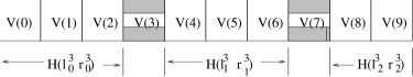
Fig. 5: A schematic diagram showing the vertices to be removed in each iteration $i$ while computing a near-optimal independent set for 1-FPN-specified planar graphs. In our example $i=3$, $l+1=4$, and $m=9$. Each box represents a copy of the vertices in the original static graph. The shaded area represents the vertices that are removed.

This completes the discussion of the approximation algorithm for 1-fpn-pl-mis. By combining the above arguments along with those in §7.2 through §7.7, we can show that several other optimization problems can be approximated in a similar fashion. Again it is easy to see that the technique extends to problems for arbitrary instances and also to problems for instances specified using $k$-narrow 1-FPN-specifications. Thus we have the following theorem.

Theorem 25.

For all fixed $k\geq 1$, $\epsilon>0$ and for all of the problems $\Pi$ stated in §7.7, there are polynomial time approximation algorithms with performance guarantee $(1+\epsilon)\cdot FBEST_{\Pi}$ for problems $\Pi$, when specified using $k$-level-restricted 1-FPN-specifications. Here $FBEST_{\Pi}$ denotes the best known performance guarantee of an algorithm for the problem $\Pi$ for instances specified using standard specifications.

Observe that the technique used to devise approximation algorithms for problems restricted to $k$-narrow 1-FPN-specified instances is very similar to the technique used to devise approximation algorithms for $k$-level-restricted L-specified problems. But there are two important differences in the details of the algorithms.

1. In case of algorithms for L-specified problems, the number of equivalence classes is $O(n)$ where $n$ is the number of nonterminals. In contrast, the number of equivalence classes in case of algorithms for 1-FPN-specified problems is only $O(1)$.

2. The size of the subgraphs for which the problem is solved near-optimally also differs significantly. Specifically, the number of explicit vertices in $PE(G_{i}^{l})$ can be $O(N^{l})$. Moreover the time required to compute $PE(G_{i}^{l})$ can be $O(N^{l+k})$. In contrast, the number of explicit vertices in each $H(l_{p}^{i},r_{p}^{i})$ is only $O(N)$ and the time required to construct each $H(l_{p}^{i},r_{p}^{i})$ is only $O(N)$. In both cases we use $N$ to be the vertex number of the respective specifications $\Gamma$ ( $N$ can be $O(size(\Gamma)$).

These important differences allow us to devise linear time approximation schemes for 1-FPN-specified problems.

8 Conclusions

8.1 Summary

We have investigated the polynomial time approximability of several PSPACE-hard optimization problems for both L- and 1-FPN-specified instances. A general approach was given to obtain polynomial time approximation schemes for several PSPACE-hard optimization problems for planar graphs specified using $k$-level-restricted L- or 1-FPN-specifications. We believe that the partial expansion technique can be used to obtain efficient approximations for other problems specified using L- or 1-FPN-specifications as well as for problems specified using other succinct specifications.

In an accompanying paper [44], we investigate the decision complexity of various combinatorial problems specified using various kinds of L-specifications and 1-FPN-specifications. There we give a general method to obtain PSPACE-hard lower bounds for such problems including the ones discussed here.

8.2 Open Problems

We conclude with a list of open problems for future research.

1. Can we use the concept of Probabilistically Checkable Debate systems [8, 9] to prove non-approximability results for problems specified using arbitrary (not level-restricted) L-specifications ?

   Recently, Agarwal and Condon [1] have partially answered this question by showing that unless P = PSPACE, there is no polynomial time approximation scheme for the problem l-max-3sat. The result was proved by using the characterization of PSPACE in terms of random debate systems. In [22], we extended their result to hold for any l-max-sat(S) such that $Rep({\bf S})$ denotes the set of all finite arity Boolean relations.

2. Recently, several researchers have considered logical definability of a number of optimization problems and defined appropriate classes such as MAX SNP MAX $\Pi_{1}$ MAX NP and MAX #P (cf. [25, 28, 51, 53]). All these researchers have assumed the the input is specified using standard specifications. What happens if the instances (finite or infinite) are specified succinctly ?

   Some work has been done along these lines by Hirst and Harel [17]. Specifically, they considered infinite recursive versions of several NP optimization problems. They prove that some problems become highly undecidable (in terms of Turing degrees) while others remain on low levels of arithmetic hierarchy. As a corollary of their results they provide a method for proving (finitary) problems to be outside the syntactic class MAX NP and hence outside MAX SNP.

Acknowledgments: We thank the referees for invaluable comments that greatly improved the presentation. We also thank Anne Condon, Ashish Naik, Egon Wanke, Joan Feigenbaum, R. Ravi, S.S. Ravi and Thomas Lengauer for many helpful conversations during the course of writing this paper.

References

- [1] S. Agarwal and A. Condon, On Approximation Algorithms for Hierarchical MAX-SAT, Proc. 10th IEEE Annual Conference on Structure in Complexity Theory, June 1995, pp. 181-190.
- [2] S. Arora, C. Lund, R. Motwani, M. Sudan and M Szegedy, Proof Verification and Hardness of Approximation Problems, Proc. 33rd IEEE Symposium on Foundations of Computer Science (FOCS), 1992, pp. 14-23.
- [3] B.S. Baker, Approximation Algorithms for NP-Complete Problems on Planar Graphs, Journal of the ACM (J. ACM), Vol. 41, No. 1, 1994, pp. 153-180.
- [4] M. Bellare, O. Goldreich and M. Sudan, Free Bits, PCPs and Non-Approximability – Towards Tight Results, Proc. 36rd IEEE Symposium on Foundations of Computer Science (FOCS’95), Oct. 1995, pp. 422-431.
- [5] J.L. Bentley, T. Ottmann and P. Widmayer, The Complexity of Manipulating Hierarchically Defined set of Rectangles, Advances in Computing Research, ed. F.P. Preparata, Vol. 1, (1983), pp. 127-158.
- [6] E. Cohen and N. Megiddo, Recognizing Properties of Periodic graphs, Applied Geometry and Discrete Mathematics, Vol. 4, The Victor Klee Festschrift, P. Gritzmann and B. Sturmfels, eds., ACM, New York, 1991, pp. 135-146.
- [7] , Strongly Polynomial-time and NC Algorithms for Detecting Cycles in Dynamic Graphs, Journal of the ACM (J. ACM) Vol. 40, No. 4, September 1993, pp. 791-830.
- [8] A. Condon, J. Feigenbaum, C. Lund and P. Shor, Probabilistically Checkable Debate Systems and Approximation Algorithms for PSPACE-Hard Functions, in Chicago Journal of Theoretical Computer Science, Vol. 1995, No. 4. http://www.cs.uchicago.edu/publications/cjtcs/articles/1995/4/contents.html. A preliminary version of the paper appears in Proc. 25th ACM Symposium on Theory of Computing (STOC), 1993, pp. 305-313.
- [9] , Random Debaters and the Hardness of Approximating Stochastic Functions, SIAM Journal on Computing, 26(2), April 1997, pp. 369-400. A preliminary version of the paper appears in Proc. 9th IEEE Annual Conference on Structure in Complexity Theory, June 1994, pp. 280-293.
- [10] D. Gale, Transient Flows in Networks, Michigan Mathematical Journal, No. 6, 1959 , pp. 59-63.
- [11] H. Galperin, Succinct Representation of Graphs, Ph.D. Thesis, Princeton University, 1982.
- [12] M.R. Garey and D.S. Johnson, Computers and Intractability. A Guide to the Theory of NP-Completeness, Freeman, San Francisco CA, 1979.
- [13] C. Ghezzi, M. Jazayeri and D. Mandrioli, Fundamentals of Software Engineering, Prentice Hall, Englewood Cliffs, NJ, 1991.
- [14] M.X. Goemans and D.P. Williamson, Improved approximation algorithms for maximum cut and satisfiability problems using semidefinite programming, Journal of the ACM (J. ACM), 42(6):1115-1145, November 1995. A preliminary version appeared as .878 Approximation Algorithms for MAX CUT and MAX 2SAT, Proc. 26th Annual ACM Symposium on Theory of Computing, (STOC), May 1994, pp. 422-431.
- [15] A. Habel and H.J. Kreowski, May we Introduce to you: Hypergraph Languages Generated by Hyperedge Replacement, Proc. 13th International Workshop on Graph-Theoretic Concepts in Computer Science (WG’87), Springer Verlag, LNCS, Vol. 291, 1987, pp. 15-26.
- [16] F.O. Hadlock, Finding a Maximum Cut in a Planar Graph in Polynomial Time, SIAM Journal on Computing, No. 4, 1975, pp. 221-225.
- [17] T. Hirst, D. Harel, Taking it to the Limit: On Infinite Variants of NP-Complete Problems, Journal of Computer and System Sciences (JCSS), 53(2), October 1996, pp. 180-193.
- [18] F. Höfting, T. Lengauer and E. Wanke, Processing of Hierarchically Defined Graphs and Graph Families, Data Structures and Efficient Algorithms (Final Report on the DFG Special Joint Initiative), Springer-Verlag, LNCS 594, 1992, pp. 44-69.
- [19] F. Höfting and E. Wanke, Minimum Cost Paths in Periodic Graphs, SIAM Journal on Computing, Vol. 24, No. 5, 1995, pp. 1051-1067.
- [20] H. B. Hunt III, M. V. Marathe, V. Radhakrishnan, S. S. Ravi, D. J. Rosenkrantz and R. E. Stearns, A Unified Approach to Approximation Schemes for NP- and PSPACE-Hard Problems for Geometric Graphs, Proc. 2nd Annual European Symposium on Algorithms (ESA’94), September, 1994, pp. 424-435. To appear in J. Algorithms.
- [21] H.B. Hunt III, M.V. Marathe, V. Radhakrishnan, D.J. Rosenkrantz and R.E. Stearns, Designing Approximation Schemes Using L-Reductions, in Proc. of the 14th Annual Foundations of Software Technology and Theoretical Computer Science (FST &TCS), Madras, India, December, 1994, pp. 342-353. A complete version of the paper titled Parallel Approximation Schemes for Planar and Near-Planar Satisfiability and Graph Problems is available as Technical Report No. LA-UR-96-2723, Los Alamos National Laboratory, 1996.
- [22] H.B. Hunt III, M.V. Marathe and R.E. Stearns, Generalized CNF Satisfiability Problems and Non-Efficient Approximability, Proc. 9th IEEE Conf. on Structure in Complexity Theory, June-July 1994, pp. 356-366. A detailed version of the paper appears as University at Albany Technical Report, TR-95-27, May 1995.
- [23] K. Iwano and K. Steiglitz, Testing for Cycles in Infinite Graphs with Periodic Structure, Proc. 19th Annual ACM Symposium on Theory of Computing, (STOC), 1987, pp. 46-53.
- [24] , Planarity Testing of Doubly Connected Periodic Infinite Graphs, Networks, No. 18, 1988, pp. 205-222.
- [25] V. Kann, On the Approximability of NP-complete Optimization Problems, Ph.D. Thesis, Dept. of Numerical Analysis and Computing Science, Royal Institute of Technology, Stockholm, Sweden, May 1992.
- [26] R.M. Karp, R.E. Miller and S. Winograd, The Organization of Computations for Uniform Recurrence Equations, Journal of the ACM (J. ACM), Vol. 14, No. 3, 1967, pp. 563-590.
- [27] M. Kodialam and J.B. Orlin, Recognizing Strong Connectivity in Periodic graphs and its relation to integer programming, Proc. 2nd ACM-SIAM Symposium on Discrete Algorithms (SODA), 1991, pp. 131-135.
- [28] P. G. Kolaitis and M.N. Thakur, Logical Definability of NP Optimization Problems, Information and Computation, No. 115, 1994, pp. 321-353.
- [29] K. R. Kosaraju and G.F. Sullivan, Detecting Cycles in Dynamic Graphs in Polynomial Time, Proc. 29th IEEE Symposium on Foundations of Computer Science (FOCS), 1988, pp. 398-406.
- [30] T. Lengauer, The Complexity of Compacting Hierarchically Specified Layouts of Integrated Circuits, Proc. 23rd IEEE Symposium on Foundations of Computer Science (FOCS), 1982, pp. 358-368.
- [31] , Exploiting Hierarchy in VLSI Design, Proc. AWOC ’86, Springer Verlag, LNCS 227, 1986, pp. 180-193.
- [32] T. Lengauer and E. Wanke, Efficient Solutions for Connectivity Problems for Hierarchically Defined Graphs, SIAM Journal on Computing, Vol. 17, No. 6, 1988, pp. 1063-1080.
- [33] T. Lengauer and C. Weiner, Efficient Solutions Hierarchical Systems of Linear Equations, Computing, Vol 39, 1987, pp. 111-132.
- [34] T. Lengauer, Efficient Algorithms for Finding Minimum Spanning Forests of Hierarchically Defined graphs, Journal of Algorithms, Vol. 8, 1987, pp. 260-284.
- [35] , Hierarchical Planarity Testing, Journal of the ACM (J. ACM), Vol. 36, No. 3, July 1989, pp. 474-509.
- [36] , Combinatorial Algorithms for Integrated Circuit Layout, John Wiley and Sons, 1990.
- [37] T. Lengauer and K.W. Wagner, The Correlation Between the Complexities of Non-Hierarchical and Hierarchical Versions of Graph Problems, Journal of Computer and System Sciences (JCSS), Vol. 44, 1992, pp. 63-93.
- [38] T. Lengauer and E. Wanke, Efficient Decision Procedures for Graph Properties on Context-Free Graph Languages, Journal of the ACM (J. ACM), Vol. 40, No. 2, 1993, pp. 368-393.
- [39] D. Lichtenstein, Planar Formulae and their Uses, SIAM Journal on Computing, Vol 11, No. 2, May 1982 , pp. 329-343.
- [40] M.V. Marathe H.B. Hunt III, and S.S. Ravi, The Complexity of Approximating PSPACE-Complete Problems for Hierarchical Specifications, Nordic Journal of Computing, Vol. 1, 1994, pp. 275-316.
- [41] M.V. Marathe, V. Radhakrishnan, H.B. Hunt III, and S.S. Ravi, Hierarchical Specified Unit Disk Graphs, in Theoretical Computer Science, 174(1-2), pp. 23-65, March 1997. A preliminary version of the paper appears in Proc. 19th International Workshop on Graph-Theoretic Concepts in Computer Science (WG ’93), June, 1993, pp. 21-32.
- [42] M.V. Marathe, H.B. Hunt III, R.E. Stearns and V. Radhakrishnan, Approximation Schemes for PSPACE-Complete Problems for Succinct Specifications, Proc. 26th ACM Annual Symposium on Theory of Computing (STOC), 1994, pp. 468-477.
- [43] M.V. Marathe, Complexity and Approximability of NP- and PSPACE-hard Optimization Problems, Ph.D. thesis, Department of Computer Science, University at Albany, Albany, NY August, 1994.
- [44] M.V. Marathe, H.B. Hunt III, R.E. Stearns and V. Radhakrishnan, Complexity of Hierarchically and 1-Dimensional Periodically Specified Problems, to appear in Proc. DIMACS Workshop on Satisfiability Problem: Theory and Applications, 1996. Also available as Technical Report LAUR-93-3348, Los Alamos National Laboratory, August, 1995.
- [45] M.V. Marathe, H.B. Hunt III and R.E. Stearns, A Uniform Approach to prove NEXPTIME-hardness for problems specified by G.C.R, S.C.R and BOW Specifications, manuscript, November 1995.
- [46] J.O. McClain, L.J. Thomas and J.B. Mazzola, Operations Management, Prentice Hall, Englewood Cliffs, 1992.
- [47] C. Mead and L. Conway, Introduction to VLSI systems, Addison Wesley, 1980.
- [48] J.B. Orlin, The Complexity of Dynamic/Periodic Languages and Optimization Problems, Sloan W.P. No. 1679-86, July 1985, Working paper, Alfred P. Sloan School of Management, MIT, Cambridge, MA 02139. A Preliminary version of the paper appears in Proc. 13th ACM Annual Symposium on Theory of Computing (STOC), 1981, pp. 218-227.
- [49] , Maximum Convex Cost Dynamic Network Flows, Mathematics for Operations Research, Vol. 9, No. 2, May 1984, pp. 190-206.
- [50] , Some Problems on Dynamic/Periodic Graphs, Progress in Combinatorial Optimization, Academic Press, May 1984, pp. 273-293.
- [51] A. Panconesi and D. Ranjan, Quantifiers and Approximations, Theoretical Computer Science, 107, 1993, pp. 145-163.
- [52] C. Papadimitriou and M. Yannakakis, A note on Succinct Representation of Graphs, Information and Computation, No. 71, 1986, pp. 181-185.
- [53] , Optimization, Approximation and Complexity Classes, Journal of Computer and System Sciences (JCSS), No. 43, 1991, pp. 425-440.
- [54] C. Papadimitriou, Computational Complexity, Addison-Wesley, Reading, Massachusetts, 1994.
- [55] D.J. Rosenkrantz and H.B. Hunt III, The Complexity of Processing Hierarchical Specifications, SIAM Journal on Computing, Vol. 22, No. 3, 1993, pp. 627-649.
- [56] T. Schaefer, The Complexity of Satisfiability Problems, Proc. 10th ACM Symposium on Theory of Computing (STOC), 1978, pp. 216-226.
- [57] K.W. Wagner, The Complexity of Problems Concerning Graphs with Regularities, Proc. 11th Symposium on Math. Foundations of Computer Science (MFCS), LNCS 176, Springer-Verlag, 1984, pp. 544-552.
- [58] E. Wanke, Paths and Cycles in Finite Periodic Graphs, Proc. 20th Symposium on Math. Foundations of Computer Science (MFCS), LNCS 711, Springer-Verlag, 1993, pp. 751-760.
- [59] M. Williams, Efficient Processing of Hierarchical Graphs, TR 90-06, Dept of Computer Science, Iowa Sate University. (Parts of the report appeared in WADS’89, pp. 563-576 and SWAT’90, pp. 320-331 coauthored with Fernandez-Baca.)
- [60] M. Yannakakis, On the Approximation of Maximum Satisfiability, J. of Algorithms, Vol. 17, 1994, pp. 475–502.