On The Capacity Of Time-Varying Channels With Periodic Feedback

Abstract

The capacity of time-varying channels with periodic feedback at the transmitter is evaluated. It is assumed that the channel state information is perfectly known at the receiver and is fed back to the transmitter at the regular time-intervals. The system capacity is investigated in two cases: i) finite state Markov channel, and ii) additive white Gaussian noise channel with time-correlated fading. In the first case, it is shown that the capacity is achievable by multiplexing multiple codebooks across the channel. In the second case, the channel capacity and the optimal adaptive coding is obtained. It is shown that the optimal adaptation can be achieved by a single Gaussian codebook, while adaptively allocating the total power based on the side information at the transmitter.

I Introduction

Communications theory over time-varying channels has been widely studied from different perspectives regarding the availability of the channel state information (CSI) at the transmitter and/or the receiver. Communication with perfect CSI at the transmitter is studied by Shannon in [1], where the capacity is expressed as that of an equivalent memoryless channel without side information at either the transmitter or the receiver. Communication with perfect CSI at the receiver is investigated, for example, in [2]. With the assumption of perfect CSI at both the transmitter and the receiver, the capacity of finite state Markov channels (FSMCs) and compound channels is studied in [3] and [4], respectively. In practice, the assumption of perfect CSI is not practical due to estimation inaccuracy, limited feedback channel capacity, or feedback delay. Communication with imperfect side information is well investigated in the literature[5, 6, 7, 8]. In [5], the capacity of FSMCs is evaluated based on the assumed statistical relationship of the channel state and side information at the transmitter. The channel capacity, when feedback delay is taken into account, is studied in [9, 10]. The optimal transmission and feedback strategies with finite feedback alphabet cardinality is investigated in [11].

In this paper, we consider a point-to-point time-varying channel with perfectly known CSI at the receiver. It is assumed that the channel is constant during a channel use and varies from one channel use to the next, based on a Markov random process. The CSI is provided at the transmitter through a noiseless feedback link at regularly-spaced time intervals. Every $T$ channel use, the CSI of the current channel use is fed back to the transmitter. We obtain the channel capacity of the system and show that it is achievable by multiplexing $T$ codebooks across the channel. It is worth mentioning that for FSMCs, the results of [5] apply directly to compute the channel capacity, if the side information at the transmitter and receiver are jointly stationary. However, in our model, the side information at the transmitter is not stationary.

Adaptive transmission is an efficient technique to increase the spectral efficiency of time-varying wireless channel by adaptively modifying the transmission rate, power, etc., according to the state of the channel seen by the receiver. Adaptive transmission, which requires accurate channel estimates at the receiver and a reliable feedback path between the receiver and transmitter, was first proposed in the late 1960’s [12]. A variable-rate and variable-power MQAM modulation scheme for high-speed data transmission over fading channels is studied in [13][14], where the transmission rate and power are optimized to maximize the spectral efficiency. We utilize the introduced feedback model to obtain the capacity of additive white Gaussian noise (AWGN) channel with time-correlated fading. It is shown that the capacity is achievable using a single codebook with adaptively allocating power based on the side information at the transmitter. Also, the optimum power allocation is derived.

The rest of the paper is organized as follows. In Section II, the system model is described and the channel capacity is obtained. The capacity of time-correlated fading channel with periodic feedback is derived in Section III. The impact of channel correlation and feedback error on the capacity is evaluated in Section IV. Finally, the paper is concluded in Section V.

Throughout this paper, upper case letters represent random variables; lower case letters denote a particular value of the random variable; $a_{m}^{n}$ represents the sequence $(a_{m},\cdots,a_{n})$ and $a^{*}$ is the complex conjugate of $a$.

II Markov Channel With Feedback State

We consider a channel with discrete input $X_{n}\in\mathcal{X}$ and discrete output $Y_{n}\in\mathcal{Y}$ at time instant $n$. The channel state is characterized as a finite-state first order Markov process:

$$\mbox{Pr}(u_{n}|u_{1}^{n-k})=\mbox{Pr}(u_{n}|u_{n-k})$$ (1)

The state process, $U_{n}\in\mathcal{U}$, is independent of the channel input and channel output:

$$\mbox{Pr}(x_{1}^{N},y_{1}^{N}|u_{1}^{N})=\prod_{n=1}^{N}\mbox{Pr}(x_{n},y_{n}|u_{n}).$$ (2)

It is assumed that CSI is perfectly known at the receiver. The CSI is provided at the transmitter through a noiseless feedback link periodically at every $T$ symbols, i.e., $U_{1},U_{T+1},U_{2T+1},\cdots$ are sent over the feedback link and instantly received at the transmitter. Assume that the codeword length, $N$, is an integer factor of $T$ and $M\triangleq\frac{N}{T}$. Let us define $V_{i}\triangleq U_{T(i-1)+1}$ for $1\leq i\leq M$ and $\tilde{n}\triangleq\lfloor\frac{n}{T}\rfloor+1$.

Encoding and Decoding

Assume that $W\in\mathcal{W}$ is the message to be sent by the transmitter and $A_{w}=2^{NR}$ is the cardinality of $\mathcal{W}$. A codeword of length $N$ is a sequence of the encoding function $\varphi_{n}$ which maps the set of messages to the channel input alphabets. The input codeword at time $n$ depends on the message $w$ and the CSI at the transmitter up to time $n$, i.e. $v_{1}^{\tilde{n}}$,

$$x_{n}=\varphi_{n}(w,v_{1}^{\tilde{n}}).$$ (3)

The decoding function, $\phi$, maps a received sequence of $N$ channel outputs using CSI at the receiver to the message set such that the decoded message is $\hat{w}=\phi(y_{1}^{N},u_{1}^{N})$.

Theorem 1

The capacity of a finite state Markov channel with periodic feedback is given by

$$\frac{1}{T}\sum_{t=1}^{T}\sum_{v}{\mathrm{Pr}}(v)\max_{q_{t}(x|v)}\sum_{u}P_{t}(u|v)I(X;Y|u,v),$$ (4)

where $T$ is the feedback period, $P_{t}(u|v)={\mathrm{Pr}}_{u_{i}|u_{i-t+1}}(u|v)$ and $q_{t}(x|v)$ is the random coding probability distribution function (PDF) parametrized with subscript $t$ to reflect the dependency on time.

II-A Achievability

We state a result on the capacity of FSMCs, which we then apply in the proof. It is shown that the capacity of FSMCs with perfectly known CSI, $U$, at the receiver and side information $V$ at the transmitter is [5]

$$C=\sum_{v}\mbox{Pr}(v)\max_{q(x|v)}\sum_{u}\mbox{Pr}(u|v)I(X;Y|u,v),$$ (5)

where $U$ and $V$ are jointly stationary and ergodic with joint PDF $\mbox{Pr}(U,V)$ and $V$ is a deterministic function of $U$.

We consider the channel as $T$ parallel subchannels where the $t^{\rm{th}}$ subchannel ($1\leq t\leq T$) occurs in time instances $(i-1)T+t,1\leq i\leq M$. Noting that the channel state of the $t^{\rm{th}}$ subchannel $\{U_{(i-1)T+t}\}_{i=1}^{M}$ and the side information at the transmitter $\{V_{i}\}_{i=1}^{M}=\{U_{(i-1)T+1}\}_{i=1}^{M}$ are jointly stationary and ergodic, we define $P_{t}(u|v)=\mbox{Pr}_{u_{i}|u_{i-t+1}}(u|v)$ for $1\leq t\leq T$. Using (5), the achievable rate of the $t^{\rm{th}}$ subchannel is

$$R_{t}=\sum_{v}\mbox{Pr}(v)\max_{q_{t}(x|v)}\sum_{u}P_{t}(u|v)I(X;Y|u,v).$$ (6)

$T$ codebooks are designed corresponding to $R_{t}$ for $1\leq t\leq T$ and multiplexed across the $T$ subchannels, i.e., at time instants $(i-1)T+t$ for $1\leq i\leq M$, the channel inputs from the $t^{\rm{th}}$ codebook are sent over the channel. Therefore, the achievable rate is

$$R=\frac{1}{T}\sum_{t=1}^{T}\sum_{v}\mbox{Pr}(v)\max_{q_{t}(x|v)}\sum_{u}P_{t}(u|v)I(X;Y|u,v).$$ (7)

II-B Converse

In this part, we prove the converse to the capacity theorem. The proof is motivated by the proof in [5]. From the Fano’s inequality[15], we have

$$H(W|Y_{1}^{N},U_{1}^{N})\leq P_{e}\log A_{w}+h(P_{e})=N\epsilon_{N},$$ (8)

where $P_{e}=\mbox{Pr}(W\neq\hat{W})$ and $\epsilon_{N}\to 0$ as $N\to\infty$.

$$H(W|Y_{1}^{N},U_{1}^{N}) = H(W|U_{1}^{N})-I(W;Y_{1}^{N}|U_{1}^{N})$$ (9)

$$= NR-I(W;Y_{1}^{N}|U_{1}^{N}).$$

Using (8) and (9), we can write

$$R\leq\frac{1}{N}I(W;Y_{1}^{N}|U_{1}^{N})+\epsilon_{N}.$$ (10)

Then we have,

$$I(W;Y_{1}^{N}|U_{1}^{N}){}$$ (11)

$$= \sum_{n=1}^{N}I(W;Y_{n}|U_{1}^{N},Y_{1}^{n-1})$$

$$= \sum_{n=1}^{N}H(Y_{n}|U_{1}^{N},Y_{1}^{n-1})-H(Y_{n}|U_{1}^{N},Y_{1}^{n-1},W)$$

$$\leq \sum_{n=1}^{N}H(Y_{n}|U_{n},V_{1}^{\tilde{n}})-H(Y_{n}|U_{1}^{N},Y_{1}^{n-1},W)$$

$$\stackrel{{\scriptstyle a}}{{\leq}} \sum_{n=1}^{N}H(Y_{n}|U_{n},V_{1}^{\tilde{n}})-H(Y_{n}|U_{n},X_{n},V_{1}^{\tilde{n}})$$

$$= \sum_{n=1}^{N}I(X_{n};Y_{n}|U_{n},V_{1}^{\tilde{n}}),$$ (12)

where ($a$) follows from the fact that the channel output is independent of the message and past channel outputs given the state of the channel and the channel input. On the other hand, for a given $n$, we have

$$I(X_{n};Y_{n}|U_{n},V_{1}^{\tilde{n}}){}$$ (13)

$$= \sum_{u_{n},v_{1}^{\tilde{n}}}\mbox{Pr}(u_{n}|v_{\tilde{n}},v_{1}^{\tilde{n}-1})\mbox{Pr}(v_{1}^{\tilde{n}-1}|v_{\tilde{n}})\mbox{Pr}(v_{\tilde{n}})I(X_{n};Y_{n}|u_{n},v_{1}^{\tilde{n}-1},v_{\tilde{n}})$$

$$\stackrel{{\scriptstyle b}}{{=}} \sum_{u_{n},v_{\tilde{n}}}\mbox{Pr}(u_{n}|v_{\tilde{n}})\mbox{Pr}(v_{\tilde{n}})\sum_{v_{1}^{\tilde{n}-1}}\mbox{Pr}(v_{1}^{\tilde{n}-1}|v_{\tilde{n}})I(X_{n};Y_{n}|u_{n},v_{1}^{\tilde{n}-1},v_{\tilde{n}})$$

$$\stackrel{{\scriptstyle c}}{{\leq}} \sum_{u_{n},v_{\tilde{n}}}\mbox{Pr}(u_{n}|v_{\tilde{n}})\mbox{Pr}(v_{\tilde{n}})\max_{q(x_{n}|v_{\tilde{n}})}I(X_{n};Y_{n}|u_{n},v_{\tilde{n}}),$$

where ($b$) follows from the property in (1), and ($c$) results from the concavity of mutual information with respect to the input distribution, and $q(x_{n}|v_{\tilde{n}})\triangleq\sum_{v_{1}^{\tilde{n}-1}}\mbox{Pr}(v_{1}^{\tilde{n}-1}|v_{\tilde{n}})\mbox{Pr}(x_{n}|v_{1}^{\tilde{n}})$. Replacing $n=(\tilde{n}-1)T+t$ in (13) and using (12), we have

$$I(W;Y_{1}^{N}|U_{1}^{N}){}$$ (15)

$$\leq \sum_{\tilde{n}=1}^{M}\sum_{t=1}^{T}\sum_{v_{\tilde{n}}}\sum_{u_{(\tilde{n}-1)T+t}}\mbox{Pr}(u_{(\tilde{n}-1)T+t}|v_{\tilde{n}})\mbox{Pr}(v_{\tilde{n}})\times$$

$$\max_{q(x_{(\tilde{n}-1)T+t}|v_{\tilde{n}})}I(X_{(\tilde{n}-1)T+t};Y_{(\tilde{n}-1)T+t}|u_{(\tilde{n}-1)T+t},v_{\tilde{n}})$$

$$= M\sum_{t=1}^{T}\sum_{u,v}P_{t}(u|v)\mbox{Pr}(v)\max_{q_{t}(x|v)}I(X;Y|u,v),$$

where (15) follows from the fact that $\{V_{i}\}_{i=1}^{M}$ and $\{U_{(i-1)T+t}\}_{i=1}^{M}$ are jointly stationary and ergodic and the right-hand side of (LABEL:fano33) does not depend on $\tilde{n}$. Using (10) and (15), we have

$$R\leq\frac{1}{T}\sum_{t=1}^{T}\sum_{v}\mbox{Pr}(v)\max_{q_{t}(x|v)}\sum_{u}P_{t}(u|v)I(X;Y|u,v)+\epsilon_{N}.$$ (16)

$\blacksquare$

III Gaussian Channel

In this section, we consider a point to point transmission over a time-correlated fading channel. It is assumed that the channel gain is constant over each channel use (symbol) and varies from symbol to symbol, following a first order Markovian random process. The signal at the receiver is

$$r_{n}=h_{n}x_{n}+z_{n},$$ (17)

where $h_{n}\in\mathbb{C}$ is the fading gain and $z_{n}$ is AWGN with zero mean and unit variance. It is assumed that the CSI is perfectly known to the receiver. Every $T$ channel use, the instantaneous fading gain is sent to the transmitter through a noiseless feedback link, i.e., $|h_{1}|,|h_{T+1}|,\cdots,|h_{(M-1)T+1}|$ are fed back and instantly received at the transmitter.

Let us define $u_{n}\triangleq|h_{n}|^{2}$ for $1\leq n\leq N$, $v_{i}\triangleq|h_{(i-1)T+1}|^{2}$ for $1\leq i\leq M$ and $P_{t}(u|v)\triangleq\mbox{Pr}_{u_{i}|u_{i-t+1}}(u|v)$. The average input power is subject to the constraint $\mathbb{E}[|x_{n}|^{2}]\leq\mathcal{P}$. In the following, $\mathbb{E}_{t}[g(U,V)]$ denotes the expectation value over $g(u,v)$ where $U$ and $V$ have joint PDF $P_{t}(u,v)$.

Theorem 2

The capacity of time-correlated fading channel with periodic feedback is

$$\max_{\overline{\rho}_{1}\cdots\overline{\rho}_{T}}\frac{1}{T}\sum_{t=1}^{T}\mathbb{E}_{t}[\log(1+U\overline{\rho}_{t}(V))],$$ (18)

subject to $\frac{1}{T}\sum_{t=1}^{T}\mathbb{E}[\overline{\rho}_{t}(V)]\leq\mathcal{P}$, where $T$ is the feedback period.

First, we recount some results on the capacity of single user channels, which is applied in the proof. A general formula for the capacity of single user channels which is not necessarily information stable or stationary is obtained in [16]. Consider input $X$ and output $Y$ as sequences of finite-dimensional distribution, where $Y$ is induced by $X$ via a channel which is an arbitrary sequence of finite-dimensional conditional output distribution from input alphabets to the output alphabets. The general formula for the channel capacity is as follows:

$$C=\sup_{X}\underline{I}(X;Y),$$ (19)

where $\underline{I}(X;Y)$ is defined as the liminf in probability of the normalized information density [16]

$$i_{N}(X_{1}^{N};Y_{1}^{N})=\frac{1}{N}\log\frac{\mbox{Pr}(Y_{1}^{N}|X_{1}^{N})}{\mbox{Pr}(Y_{1}^{N})}.$$ (20)

Assume that the channel state information, $Q$, is available at the receiver. Considering $Q$ as an additional output, the channel capacity is $C=\sup_{X}\underline{I}(X;Y,Q)$. If $Q$ is not available at the transmitter and is consequently independent of $X$, then the capacity is [17]

$$C=\sup_{X}\underline{I}(X;Y|Q),$$ (21)

where $\underline{I}(X;Y|Q)$ is the liminf in probability of the normalized conditional information density

$$i_{N}(X_{1}^{N};Y_{1}^{N}|Q_{1}^{N})=\frac{1}{N}\log\frac{\mbox{Pr}(Y_{1}^{N}|X_{1}^{N},Q_{1}^{N})}{\mbox{Pr}(Y_{1}^{N}|Q_{1}^{N})}.$$ (22)

Now, we are ready to prove Theorem 2, where the proof is motivated by the proof in [5].

III-A Achievability

Noting (17), the processed received signal at time $n$ is

$$y_{n}=r_{n}\frac{h_{n}^{*}}{|h_{n}|}=|h_{n}|x_{n}+z^{\prime}_{n},$$ (23)

where $z^{\prime}_{n}=\frac{h_{n}^{*}}{|h_{n}|}z_{n}$, which has the same distribution as $z_{n}$. The transmitter sends

$$x_{n}=\sqrt{\rho_{n}(v_{\tilde{n}})}s_{n},$$ (24)

over the channel where $s_{n}$ is an i.i.d. Gaussian codebook with zero mean and unit variance, and $\rho_{n}:\mathbb{R}_{+}\to\mathbb{R}_{+}$ is the power allocation function. Using (23) and (24), we can write

$$y_{n}=\sqrt{q_{n}}s_{n}+z^{\prime}_{n},$$ (25)

where $q_{n}=\rho_{n}(v_{\tilde{n}})|h_{n}|^{2}=\rho_{n}(v_{\tilde{n}})u_{n}$. Noting (25), we have a channel with input $S$ and output $Y$ and channel state $Q$, which is known at the receiver. Since $Q_{1}^{N}$ is independent of $S_{1}^{N}$, we can use (21) to obtain the achievable rate.

$$i_{N}(S_{1}^{N};Y_{1}^{N}|Q_{1}^{N}) = \frac{1}{N}\log\frac{\mbox{Pr}(Y_{1}^{N}|S_{1}^{N},Q_{1}^{N})}{\mbox{Pr}(Y_{1}^{N}|Q_{1}^{N})}$$ (26)

$$\stackrel{{\scriptstyle d}}{{=}} \frac{1}{N}\sum_{n=1}^{N}\log\frac{\mbox{Pr}(Y_{n}|S_{n},Q_{n})}{\mbox{Pr}(Y_{n}|Q_{n})}$$

$$= \frac{1}{N}\sum_{n=1}^{N}\left(\log(1+Q_{n})+\frac{|Y_{n}|^{2}}{1+Q_{n}}-|Z^{\prime}_{n}|^{2}\right),$$

where $(d)$ results from the fact that $S_{1}^{N}$ and ${Z^{\prime}}_{1}^{N}$ are i.i.d. sequences and the last line follows from the fact that $Y_{n}$ conditioned on $Q_{n}$ is Gaussian with zero mean and variance $1+Q_{n}$. Note that as $N\to\infty$, $\frac{1}{N}\sum_{n=1}^{N}\frac{|Y_{n}|^{2}}{1+Q_{n}}=\frac{1}{N}\sum_{n=1}^{N}|Z^{\prime}_{n}|^{2}=1$ with probability one. Therefore, with probability one, we have

$$i_{N}(S_{1}^{N};Y_{1}^{N}|Q_{1}^{N}){}$$ (27)

$$= \frac{1}{N}\sum_{n=1}^{N}\log(1+Q_{n})$$

$$= \frac{1}{MT}\sum_{t=1}^{T}\sum_{i=1}^{M}\log(1+Q_{(i-1)T+t})$$

$$= \frac{1}{T}\sum_{t=1}^{T}\frac{1}{M}\sum_{i=1}^{M}\log\left(1+U_{(i-1)T+t}\rho_{(i-1)T+t}(V_{i})\right).$$

Noting that $\{U_{(i-1)T+t}\}_{i=1}^{M}$ and $\{V_{i}\}_{i=1}^{M}$ are jointly stationary and ergodic for $1\leq t\leq T$, we define $P_{t}(u,v)$ to be their joint PDF. We set $\rho_{(i-1)T+t}=\overline{\rho}_{t}$ for $1\leq i\leq M$ and $1\leq t\leq T$. As $M\to\infty$ in (27), the sample mean converges in probability to the expectation. Therefore, the achievable rate is

$$R=\frac{1}{T}\sum_{t=1}^{T}\mathbb{E}_{t}[\log(1+U\overline{\rho}_{t}(V))].$$ (28)

III-B Converse

Using (11), we have

$$I(W;Y_{1}^{N}|U_{1}^{N}) \leq \sum_{n=1}^{N}H(Y_{n}|U_{n},V_{1}^{\tilde{n}})-H(Y_{n}|U_{n},X_{n},V_{1}^{\tilde{n}})$$ (29)

$$\leq \sum_{n=1}^{N}\mathbb{E}[\log(1+U_{n}\mathbb{E}[|X_{n}|^{2}|V_{1}^{\tilde{n}}])].$$

The above inequality relies on the facts that

$$H(Y_{n}|U_{n},X_{n},V_{1}^{\tilde{n}})=H(Z_{n})=\log 2\pi e$$ (30)

and

$$H(Y_{n}|U_{n},V_{1}^{\tilde{n}})\leq\mathbb{E}[\log(2\pi e(1+U_{n}\mathbb{E}[|X_{n}|^{2}|V_{1}^{\tilde{n}}]))].$$ (31)

The upper-bound in (31) is achieved if $X_{n}$ conditioned on $V_{1}^{\tilde{n}}$ has a Gaussian distribution. We set $x_{n}=\sqrt{f_{n}(v_{1}^{\tilde{n}})}s_{n}$ where $f_{n}:\mathbb{R}_{+}^{\tilde{n}}\to\mathbb{R}_{+}$ and $S_{1}^{N}$ is an i.i.d. Gaussian sequence with zero mean and unit variance. On the other hand,

$$\mathbb{E}[\log(1+U_{n}f_{n}(V_{1}^{\tilde{n}}))] = \mathbb{E}[\mathbb{E}[\log(1+U_{n}f_{n}(V_{1}^{\tilde{n}}))|U_{n},V_{\tilde{n}}]]$$ (32)

$$\stackrel{{\scriptstyle d}}{{\leq}} \mathbb{E}[\log(1+\mathbb{E}[U_{n}f_{n}(V_{1}^{\tilde{n}})|U_{n},V_{\tilde{n}}])]$$

$$= \mathbb{E}[\log(1+U_{n}\mathbb{E}[f_{n}(V_{1}^{\tilde{n}})|V_{\tilde{n}}])],$$

where $(d)$ follows from the concavity of the logarithm. Let us define $\rho_{n}(V_{\tilde{n}})\triangleq\mathbb{E}[f_{n}(V_{1}^{\tilde{n}}))|V_{\tilde{n}}]$. By using (29) and (32), we obtain

$$\frac{1}{N}I(W;Y_{1}^{N}|U_{1}^{N}){}$$ (33)

$$\leq \frac{1}{N}\sum_{n=1}^{N}\mathbb{E}[\log(1+U_{n}\rho_{n}(V_{\tilde{n}}))]$$

$$= \frac{1}{T}\sum_{t=1}^{T}\frac{1}{M}\sum_{i=1}^{M}\mathbb{E}[\log(1+U_{(i-1)T+t}\rho_{(i-1)T+t}(V_{i}))]$$

$$\leq \frac{1}{T}\sum_{t=1}^{T}\mathbb{E}[\log(1+\frac{1}{M}\sum_{i=1}^{M}U_{(i-1)T+t}\rho_{(i-1)T+t}(V_{i}))].$$

Using (33) and noting the fact that that $\{U_{(i-1)T+t}\}_{i=1}^{M}$ and $\{V_{i}\}_{i=1}^{M}$ are jointly stationary and ergodic for $1\leq t\leq T$, we can write

$$\frac{1}{N}I(W;Y_{1}^{N}|U_{1}^{N}) \leq \frac{1}{T}\sum_{t=1}^{T}\mathbb{E}_{t}[\log(1+U\overline{\rho}_{t}(V))],$$ (34)

where $\overline{\rho}_{t}(.)\triangleq\frac{1}{M}\sum_{i=1}^{M}\rho_{(i-1)T+t}(.)$. Combining (10) and (34), we conclude that

$$R\leq\frac{1}{T}\sum_{t=1}^{T}\mathbb{E}_{t}[\log(1+U\overline{\rho}_{t}(V))],$$ (35)

subject to $\frac{1}{T}\sum_{t=1}^{T}\mathbb{E}[\overline{\rho}_{t}(V)]\leq\mathcal{P}$.

$\blacksquare$

Remark: In Section II, we prove that the capacity of Markov channels is generally achieved by using multiple code multiplexing technique. However, for AWGN channel with time-correlated fading, the proof relies on using one Gaussian codebook, where the symbols are adaptively scaled by the appropriate power allocation function based on the side information at the transmitter.

IV Performance Evaluation

We study the impact of the channel correlation and feedback period on the capacity of the time-correlated Rayleigh fading channel. Let us assume that time-correlated Rayleigh fading channel is a Markov random process with the following PDF[18]:

$$\mbox{Pr}(u)=\left\{\begin{array}[]{ll}e^{-u}&u\geq 0\\ 0.&\textrm{otherwise}\end{array}\right.$$ (38)

$$P_{1}(u|v) = \delta(v)$$

$$P_{t}(u|v) = \Phi(u,v,\alpha^{t-1}),$$ (39)

where

$$\scriptstyle{\Phi(u,v,\sigma)=\left\{\begin{array}[]{ll}\frac{1}{1-\sigma^{2}}\exp\left(-\frac{u+\sigma^{2}v}{1-\sigma^{2}}\right)\mathcal{I}_{0}(\frac{2\sigma\sqrt{uv}}{1-\sigma^{2}})&u\geq 0,\\ 0&\textrm{otherwise.}\end{array}\right.}$$ (42)

In (42), $0<\sigma<1$ describes the channel correlation coefficient and $\mathcal{I}_{0}(.)$ denotes the modified Bessel function of order zero. Noting that the capacity in (18) is a strictly concave region of $\overline{\rho}_{t},1\leq t\leq T$, we numerically solve the convex optimization problem. In Figure 1, the capacity is depicted versus the feedback period for various channel correlation coefficients and compared to the capacity when no CSI is available at the transmitter.

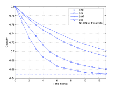
Figure 1: Capacity of time-correlated Rayleigh fading channel versus $T$ for $\mbox{SNR}=1$ and channel correlation coefficients $\alpha=0.97,0.95,0.9,0.8$. The dash-dot line is the capacity with no side information at the transmitter.

V Conclusion

We have obtained the capacity of finite state Markov channel with periodic feedback at the transmitter. Also, the channel capacity and optimal adaptive coding is derived for the time-correlated fading channel with periodic feedback. It is shown that the optimal adaptation can be achieved by a single Gaussian codebook, while scaling by the appropriate power.

References

- [1] C. E. Shannon, “Channels with side information at the transmitter,” IBM J. Res. Devel., no. 289-293, 1958.
- [2] L. H. Ozarow, S. Shamai, and A. D. Wyner, “Information theoretic considerations for cellular mobile radio,” IEEE Trans. Veh. Technology, vol. 43, pp. 359–378, May 1994.
- [3] A. Goldsmith and P. Varaiya, “Capacity of fading channels with channel side information,” IEEE Trans. Inform. Theory, vol. 43, pp. 1986–1992, Nov. 1997.
- [4] J. Wolfowitz, Coding Theorems of Information Theory. New York: Springer-Verlag, 1978.
- [5] G. Caire and S. Shamai, “On the capacity of some channels with channel state information,” IEEE Trans. Inform. Theory, vol. 45, pp. 2007 – 2019, Sept. 1999.
- [6] S. Gelfand and M. Pinsker, “Coding for channels with random parameters,” Probl. Control Inform. Theory, vol. 9, pp. 19–31, 1980.
- [7] M. Medard and R. Srikant, “Capacity of nearly-decomposable markovian fading channels under asymmetric receiver-sender side information,” in Int. Symp. Inform. Theory, p. 413, 2000.
- [8] T. E. Klein, “Capacity of Gaussian noise channels with side information and feedback,” Ph.D. thesis, MIT, Feb. 2001.
- [9] V. K. N. Lau, “Channel capacity and error exponents of variable rate adaptive channel coding for rayleigh fading channels,” IEEE Trans. Commun., vol. 47, pp. 1345 – 1356, Sept. 1999.
- [10] H. Viswanathan, “Capacity of markov channels with receiver CSI and delayed feedback,” IEEE Trans. Inform. Theory, vol. 45, pp. 761 – 771, March 1999.
- [11] Vincent K. N. Lau, Youjian Liu, and Tai-Ann Chen, “Capacity of memoryless channels and block-fading channels with designable cardinality-constrained channel state feedback,” IEEE Trans. Inform. Theory, vol. 50, pp. 2038 – 2049, Sept. 2004.
- [12] J. F. Hayes, “Adaptive feedback communications,” IEEE Trans. Commun. Technol., vol. COM-16, pp. 29–34, Feb. 1968.
- [13] Goldsmith, A.J.; Soon-Ghee Chua, “Variable-rate variable-power MQAM for fading channels,” IEEE Trans. Commun., vol. 45, pp. 1218 – 1230, Oct. 1997.
- [14] A. Goldsmith and S. Chua, “Adaptive coded modulation for fading channels,” IEEE Trans. Commun., vol. 46, pp. 595–602, May 1998.
- [15] R. G. Galager, Information theory and Reliable communication. J. Wiley, New York, 1968.
- [16] S. Verdu and T. S. Han, “A general formula for channel capacity,” IEEE Trans. Infor. Theory, vol. 40, pp. 1147–1157, July 1994.
- [17] A. Das and P. Narayan, “On the capacities of a class of finite-state channels with side information,” in Proc. CISS’98, March 1998.
- [18] A. N. Trofimov, “Convolutional codes for channels with fading,” in Proc. Inform Transmission, vol. 27, pp. 155–165, Oct. 1991.