Pragmatic Space-Time Trellis Codes for Block Fading Channels

Abstract

A pragmatic approach for the construction of space-time codes over block fading channels is investigated. The approach consists in using common convolutional encoders and Viterbi decoders with suitable generators and rates, thus greatly simplifying the implementation of space-time codes.

For the design of pragmatic space-time codes a methodology is proposed and applied, based on the extension of the concept of generalized transfer function for convolutional codes over block fading channels. Our search algorithm produces the convolutional encoder generators of pragmatic space-time codes for various number of states, number of antennas and fading rate.

Finally it is shown that, for the investigated cases, the performance of pragmatic space-time codes is better than that of previously known space-time codes, confirming that they are a valuable choice in terms of both implementation complexity and performance.

I Introduction

It is known since many years that the use of multiple receiving antennas, sufficiently spaced apart each other to obtain independent copies of the transmitted signal, is an efficient way to mitigate the effects of multipath propagation (see, e.g., [1, 2, 3]). However, only recently it has been realized that even the use of multiple transmitting antennas can give similar improvements [4, 5, 6]. With the introduction of space-time codes (STC) it has been shown how, with the use of proper trellis codes, multiple transmitting antennas can be exploited to improve system performance obtaining both diversity and coding gain, without sacrificing spectral efficiency [6, 7, 8, 9, 10, 11].

In particular, the design of STC over quasi-static flat fading (i.e., fading level constant over a frame and independent frame by frame) has been addressed in [8], where some handcrafted trellis codes for two transmitting antennas have been proposed. A number of extensions of this work have eventually appeared in the literature to design good codes for different scenarios, and STC with improved coding gain have been presented in [12, 13, 14]. In [15] it is pointed out that the diversity achievable by STC for binary phase shift keying (BPSK) and quaternary phase shift keying (QPSK) modulations can also be investigated by a binary design criteria, instead of looking for the distances among complex transmitted sequences. This approach has been extended to multiple input multiple output (MIMO) block fading channels (BFC) in [16].

The determination of the STC with maximum diversity gain and largest coding gain remains a difficult task, especially for a large number of transmitting antennas and trellis code states. Moreover, the design of STC for fast fading channels is still an open problem.

In this paper we present an approach to STC to simplify the encoder and decoder structures, that also allows a feasible method to search for good codes in BFC [17, 18, 19]. In fact, a criterion to achieve maximum diversity is given in [8], where, however, coding gain optimization is not addressed. Moreover, the STC in [8] require ad-hoc encoders and decoders. For these reasons, we present another possible approach to space-time coding, denominated pragmatic space-time codes (P-STC) [20]. Here, the “pragmatic” approach (the name following [21]) consists in the use of common convolutional encoders and Viterbi decoders over multiple transmitting and receiving antennas. We show that P-STC achieve maximum diversity and excellent performance, with no need of specific encoder or decoder different from those used for convolutional codes (CC); the Viterbi decoder requires only a simple modification in the metrics computation.

We use the BFC model to investigate the design and the performance of STC. The BFC represents a simple and powerful model to include a variety of fading rates, from ”fast” fading (i.e., ideal symbol interleaving) to quasi-static.

Here, after the proposal of the P-STC structure, we first derive the pairwise error probability (PEP) of STC over block fading channels. Then, we propose a method based on suitable error trellis diagrams and generalized transfer function to evaluate a bound on the performance of STC over BFC, with a discussion on geometrical uniformity over the BFC.

A new algorithm for searching good P-STC over BFC is then presented and applied to obtain the optimum (with respect to our performance bound) convolutional generators for various constraint lengths and fading rates. The numerical results, which compares our P-STC with the best known STC, confirm the validity of the approach.

For simplicity we will focus on the BPSK and QPSK modulation formats, but the extension to other formats such as M-ary quadrature amplitude modulation (M-QAM) is straightforward.

The paper is organized as follows: in section II the channel model and the general architecture of a system with STC are described; in section III the P-STC are presented; in section IV the PEP for STC over BFC is derived; in section V the frame error probability for STC over BFC is analyzed; in section VI the search methodology for P-STC in BFC is illustrated; in section VII numerical results are provided, followed by the conclusions in section VIII.

II System architecture and channel model

The general low-pass equivalent scheme for space time codes is depicted in Fig. 1, where $n$ and $m$ denote the number of transmitting and receiving antennas, respectively.

We indicate with ${\bf C}^{(t)}=\left[c_{1}^{(t)},\ldots,c_{n}^{(t)}\right]^{T}$ a super-symbol, that is a vector of symbols simultaneously transmitted at discrete time $t$ on the $n$ antennas, each having unitary norm and generated according to the modulation format by proper mapping. Thus, $n$ symbols are sent in parallel on the $n$ transmitting antennas. A codeword is a sequence $\underline{c}=\left({\bf C}^{(1)},\ldots,{\bf C}^{(N)}\right)$ of $N$ super-symbols generated by the encoder.

This codeword $\underline{c}$ is first interleaved (we refer to intra-codeword interleaving) to obtain the sequence $\underline{c}_{I}={\mathcal{I}}(\underline{c})=\left({\bf C}^{(\sigma_{1})},\ldots,{\bf C}^{(\sigma_{N})}\right)$, where $\sigma_{1},\ldots,\sigma_{N}$ is a permutation of the integers $1,\ldots,N$ and ${\mathcal{I}}(\cdot)$ is the interleaving function.

The channel model includes additive white gaussian noise (AWGN) and multiplicative flat fading, with Rayleigh distributed amplitudes assumed constant over blocks of $B$ consecutive transmitted space-time symbols and independent from block to block [17, 18, 19]. Perfect channel state information is assumed at the decoder.

The transmitted super-symbol at time $\sigma_{t}$ goes through the channel described by the $(n\times m)$ channel matrix ${\bf H}^{(\sigma_{t})}=\left\{h_{i,s}^{(\sigma_{t})}\right\}$ with ${i=1,\ldots,n;\ s=1,\ldots,m}$, where $h_{i,s}^{(\sigma_{t})}$ is the channel gain between transmitting antenna $i$ and receiving antenna $s$ at time $\sigma_{t}$.

In the BFC model these channel matrices do not change for $B$ consecutive transmissions, so that we actually have only $L=N/B$ possible distinct channel matrix instances per codeword. By denoting with ${\bf\mathcal{Z}}=\left\{{\bf Z}_{1},\ldots,{\bf Z}_{L}\right\}$ the set of $L$ channel instances, we have

$${\bf H}^{(\sigma_{t})}={\bf Z}_{l}\qquad{\text{for}}\ \sigma_{t}=(l-1)B+1,...,lB\qquad,\qquad\ l=1,\ldots,L\,.$$ (1)

When the fading block length, $B$, is equal to one, we have the ideally interleaved fading channel (i.e., independent fading levels from symbol to symbol), while for $L=1$ we have the quasi-static fading channel (fading level constant over a codeword); by varying $L$ we can describe channels with different correlation degrees [17, 18, 19].

At the receiving side the sequence of received signal vectors is $\underline{r}_{I}=\left({\bf R}^{(\sigma_{1})},\ldots,{\bf R}^{(\sigma_{N})}\right)$, and after de-interleaving we have $\underline{r}={{\mathcal{I}}^{-1}}(\underline{r}_{I})=\left({\bf R}^{(1)},\ldots,{\bf R}^{(N)}\right)$, where the received vector at time $t$ is ${\bf R}^{(t)}=\left[r_{1}^{(t)}r_{2}^{(t)}\cdots r_{m}^{(t)}\right]^{T}$ with components

$$r_{s}^{(t)}=\sqrt{E_{s}}\sum_{i=1}^{n}h_{i,s}^{(t)}c_{i}^{(t)}+\eta_{s}^{(t)},\;\;\;\;\;s=1,\ldots,m\,.$$ (2)

In this equation $r_{s}^{(t)}$ is the signal-space representation of the signal received by antenna $s$ at time $t$, the noise terms $\eta_{s}^{(t)}$ are independent, identically distributed (i.i.d.) complex Gaussian random variables, with zero mean and variance $N_{0}/2$ per dimension, and the r.v.s $h_{i,s}^{(t)}$ represent the de-interleaved complex Gaussian fading coefficients. Since we assume spatially uncorrelated channels, these are i.i.d. with zero mean and variance $1/2$ per dimension, and, consequently, $|h_{i,s}^{(t)}|$ are Rayleigh distributed r.v.s with unitary power. The constellations are multiplied by a factor $\sqrt{E_{s}}$ in order to have a transmitted energy per symbol equal to $E_{s}$, which is also the average received symbol energy (per transmitting antenna) due to the normalization adopted on fading gains.

The total energy transmitted per super-symbol is $E_{s_{T}}=nE_{s}$ and the energy transmitted per information bit is $E_{b}=E_{s}/(hR)$ where $h$ is the number of bits per modulation symbol and $R$ is the code-rate. Thus, with ideal pulse shaping the spectral efficiency is $nhR$  $[bps/Hz]$.

For the discussion in the following sections it is worthwhile to recall that, over a Rayleigh fading channel, the system achieves a diversity $\mathcal{D}$ if the asymptotic error probability is $P_{e}\approx{K}{\left(\frac{E_{s}}{N_{0}}\right)^{-\mathcal{D}}}$ where $K$ is a constant depending on the asymptotic coding gain [1, 22]. In other words, a system with diversity $\mathcal{D}$ is described by a curve of error probability with a slope approaching $10/\mathcal{D}$ [dB/decade] for large signal-to-noise ratio (SNR).

III A Pragmatic approach to space-time codes

In this section we present what we called pragmatic space-time codes, a low-complexity architecture for STC that allows an easy code design and optimization over fading channels [20]. The ”pragmatic” approach consists in using common convolutional codes as space-time codes, with the architecture presented in Fig. 2. Here, $k$ information bits are encoded by a convolutional encoder with rate $k/(nh)$. The $nh$ output bits are divided into $n$ streams, one for each transmitting antenna, of BPSK ($h=1$) or QPSK ($h=2$) symbols that are obtained from a natural (Gray) mapping of $h$ bits. By natural mapping we mean that for BPSK an information bit $b\in\{0,1\}$ is mapped into the antipodal symbol $c=2b-1$, giving $c\in\{-1,+1\}$; for QPSK a pair of information bits $a,b$ is mapped into a complex symbol $c=(2a-1)/\sqrt{2}+j(2b-1)/\sqrt{2}$, giving $c\in\{\pm 1/\sqrt{2}\pm j/\sqrt{2}\}$, with $j=\sqrt{-1}$. Then, each stream of symbols is eventually interleaved.

We indicate the STC obtained with this scheme as $(nh,k,\mu)$ $n$-P-STC, where $\mu$ is the encoder constraint length and the associated trellis has $N_{s}=2^{k(\mu-1)}$ states. For example, we report in Fig. 3 the four states (2,1,3) $2$-P-STC encoder scheme for $n=2$ transmitting antennas and BPSK modulation, obtained with a rate $1/2$ convolutional encoder with generator polynomials $(5,7)_{8}$. We can describe P-STC by using the trellis of the encoder (the same as for the CC), labelling the generic branch from state $S_{i}$ to state $S_{j}$ with the super-symbol $\widetilde{\bf C}_{S_{i}\rightarrow S_{j}}=[\widetilde{c}_{1},\ldots,\widetilde{c}_{n}]^{T}$, where for BPSK $\widetilde{c}_{l}$ is the output of the $l-th$ generator (in antipodal version). In Fig. 4 we report the trellis for the P-STC in Fig. 3.

Similarly, in Fig. 5 we report the $4$ states (4,2,2) 2-P-STC encoder scheme for $n=2$ transmitting antennas and QPSK modulation, obtained with a rate $2/4$ convolutional encoder with generator polynomials $(06,13,11,16)_{8}$.

It is clear now that with the pragmatic architecture the maximum likelihood (ML) decoder is the usual Viterbi decoder for the convolutional encoder adopted (same trellis), with a simple modification of the branch metrics. For example, in Fig. 6 we show the receiver architecture for the previous P-STC, that simply consists in the usual Viterbi decoder for the convolutional code adopted in transmission, with the only change that the metric on a generic trellis branch is $\sum_{s=1}^{m}|r_{s}^{(t)}-\sqrt{E_{s}}\left(h^{(t)}_{1,s}\widetilde{c}_{1}+h^{(t)}_{2,s}\widetilde{c}_{2}\right)|^{2}$, being $\left\{\widetilde{c}_{i}\right\}$ the set of length $n$ of the output symbols labelling the branch. In general, for $n$ transmitting antennas, the branch metric for the Viterbi decoder is

$$\sum_{s=1}^{m}|r_{s}^{(t)}-\sqrt{E_{s}}\sum_{i=1}^{n}h^{(t)}_{i,s}\widetilde{c_{i}}|^{2}\,.$$ (3)

Thus, we can resume the advantages of P-STC with respect to STC as in the following:

• the encoder is a common convolutional encoder;

• the (Viterbi) decoder is the same as for a convolutional code, except for a change in the metric evaluation;

• P-STC are easy to study and optimize, even over BFC.

These aspects will be further investigated in the next sections.

IV The pairwise error probability for space-time codes over BFC

In this section we address the performance analysis for the general class of STC over BFC.

Given the transmitted codeword $\underline{c}$, the PEP, that is the probability that the ML decoder chooses the codeword $\underline{g}\neq\underline{c}$, conditional to the set of fading levels ${\bf\mathcal{Z}}$, can be written as

$${\mathbb{P}}\left\{{\underline{c}\rightarrow\underline{g}|{\bf\mathcal{Z}}}\right\}=\frac{1}{2}\ \text{erfc}\sqrt{\frac{E_{s}}{4N_{0}}d^{2}\left(\underline{c},\underline{g}|{\bf\mathcal{Z}}\right)}\,,$$ (4)

where $\text{erfc}(x)\triangleq\frac{2}{\sqrt{\pi}}\int_{x}^{\infty}e^{-t^{2}}dt$ is the complementary Gaussian error function, and the conditional Euclidean squared distance at the channel output, $d^{2}\left(\underline{c},\underline{g}|{\bf\mathcal{Z}}\right)$, is given by [8]

$$d^{2}\left(\underline{c},\underline{g}|{\bf\mathcal{Z}}\right)=\sum_{t=1}^{N}\sum_{s=1}^{m}\left|\sum_{i=1}^{n}h_{i,s}^{(t)}\cdot\left(c_{i}^{(t)}-g_{i}^{(t)}\right)\right|^{2}\,.$$ (5)

To specialize this expression to the BFC we first rewrite the squared distance as follows

$$d^{2}\left(\underline{c},\underline{g}|{\bf\mathcal{Z}}\right) = \sum_{t=1}^{N}\sum_{s=1}^{m}{\bf h}_{s}^{(t)}\left({\bf C}^{(t)}-{\bf G}^{(t)}\right)\cdot\left({\bf C}^{(t)}-{\bf G}^{(t)}\right)^{H}{\bf h}_{s}^{(t)H\,}$$ (6)

$$= \sum_{t=1}^{N}\sum_{s=1}^{m}{\bf h}_{s}^{(t)}{{\bf A}}^{(t)}(\underline{c},\underline{g}){\bf h}_{s}^{(t)H\,}\,,$$

where ${\bf h}_{s}^{(t)}=\left[h_{1,s}^{(t)},h_{2,s}^{(t)},...,h_{n,s}^{(t)}\right]$ is the $(1\times n)$ vector of the fading coefficients related to the receiving antenna $s$, and ${\bf C}^{(t)},{\bf G}^{(t)}$ are the super-symbols at time $t$ in the sequence $\underline{c},$ and $\underline{g}$, respectively. In (6) the ($n\times n$) matrix

$${{\bf A}}^{(t)}(\underline{c},\underline{g})=\left({\bf C}^{(t)}-{\bf G}^{(t)}\right)\left({\bf C}^{(t)}-{\bf G}^{(t)}\right)^{H}$$

with elements

$$A^{(t)}_{p,q}=\left(c_{p}^{(t)}-g_{p}^{(t)}\right)\left(c_{q}^{(t)}-g_{q}^{(t)}\right)^{*}$$

is Hermitian and non-negative definite.

Due to the BFC assumption, for each frame and each receiving antenna the fading channel is described by only $L$ different vectors ${\bf h}_{s}^{(t)}\in\left\{{\bf z}_{s}^{(1)},{\bf z}_{s}^{(2)},\ldots,{\bf z}_{s}^{(L)}\right\}$ , $s=1,\ldots,m$, where ${\bf z}_{s}^{(l)}$ is the $s$-th row of ${\bf Z}_{l}$. By grouping these vectors, we can rewrite (6) as

$$d^{2}\left(\underline{c},\underline{g}|{\bf\mathcal{Z}}\right)=\sum_{l=1}^{L}\sum_{s=1}^{m}{\bf z}_{s}^{(l)}{{\bf F}}^{(l)}(\underline{c},\underline{g}){\bf z}_{s}^{(l)\,H}\,,$$ (7)

where

$${{\bf F}}^{(l)}(\underline{c},\underline{g})\triangleq\sum_{t\in T(l)}{{\bf A}}^{(t)}(\underline{c},\underline{g})=\sum_{t\in T(l)}\left({\bf C}^{(t)}-{\bf G}^{(t)}\right)\cdot\left({\bf C}^{(t)}-{\bf G}^{(t)}\right)^{H}\,\,\,l=1,\ldots,L$$ (8)

and $T(l)\triangleq\{t:{\bf H}^{(\sigma_{t})}={\bf Z}_{l}\}$ is the set of indexes $t$ where the channel fading gain matrix is equal to ${\bf Z}_{l}$. This set depends on the interleaving strategy adopted. Note that in our scheme (Fig. 2) the interleaving is done “horizontally” for each transmitting antenna and that the set $T(l)$ is independent on $s$, that means, in other words, that the interleaving rule is the same for all antennas.

The matrix ${{\bf F}}^{(l)}(\underline{c},\underline{g})$ is also Hermitian non-negative definite, being the sum of Hermitian non-negative definite matrices. It has, therefore, real non-negative eigenvalues. Moreover, it can be written as ${{\bf F}}^{(l)}(\underline{c},\underline{g})={{\bf U}}^{(l)}{{\bf\Lambda}}^{(l)}{{\bf U}}^{(l)H}$, where ${{\bf U}}^{(l)}$ is a unitary matrix and ${{\bf\Lambda}}^{(l)}$ is a real diagonal matrix, whose diagonal elements $\lambda_{i}^{(l)}$ with $i=1,\ldots,n$ are the eigenvalues of ${{\bf F}}^{(l)}(\underline{c},\underline{g})$ counting multiplicity. Note that ${{\bf F}}^{(l)}$ and its eigenvalues $\lambda_{i}^{(l)}$ are a function of $\underline{c}-\underline{g}$. As a result, we can express the squared distance $d^{2}\left(\underline{c},\underline{g}|{\bf\mathcal{Z}}\right)$ by utilizing the eigenvalues of ${{\bf F}}^{(l)}(\underline{c},\underline{g})$ as follows:

$$d^{2}\left(\underline{c},\underline{g}|{\bf\mathcal{Z}}\right) = \sum_{l=1}^{L}\sum_{s=1}^{m}{\bf z}_{s}^{(l)}{{\bf U}}^{(l)}{{\bf\Lambda}}^{(l)}{{\bf U}}^{(l)H}{\bf z}_{s}^{(l)\,H}$$ (9)

$$= \sum_{l=1}^{L}\sum_{s=1}^{m}{\bf B}_{s}^{(l)}{{\bf\Lambda}}^{(l)}{\bf B}_{s}^{(l)\,H}$$

$$= \sum_{l=1}^{L}\sum_{s=1}^{m}\sum_{i=1}^{n}\lambda_{i}^{(l)}\left|\beta_{i,s}^{(l)}\right|^{2}$$

where ${\bf B}_{s}^{(l)}=\left[\beta_{1,s}^{(l)},\beta_{2,s}^{(l)},...,\beta_{n,s}^{(l)}\right]={\bf z}_{s}^{(l)}{{\bf U}}^{(l)}$.

The difference between (9) and the similar expression reported in [8] is that, through (8), the eigenvalues in (9) are referred to the portions of the coded sequences with a given fading level.

Since ${{\bf U}}^{(l)}$ represents a unitary transformation, ${\bf B}_{s}^{(l)}$ has the same statistical description of ${\bf z}_{s}^{(l)}$. Hence, in the case of Rayleigh distribution, ${\bf B}_{s}^{(l)}$ has independent, complex Gaussian elements, with zero mean and variance 1/2 per dimension. Moreover, for BFC, vectors ${\bf B}_{s}^{(l)}$ and ${\bf B}_{s}^{(j)}$ are independent $\forall l\neq j$. Hence, the unconditional PEP becomes

$${\mathbb{P}}\left\{{\underline{c}\rightarrow\underline{g}}\right\}={\mathbb{E}}\left\{{\frac{1}{2}\text{erfc}\sqrt{\frac{E_{s}}{4N_{0}}\sum_{s=1}^{m}\sum_{l=1}^{L}\sum_{i=1}^{n}\lambda_{i}^{(l)}\left|\beta_{i,s}^{(l)}\right|^{2}}}\right\}$$ (10)

where ${\mathbb{E}}\left\{{.}\right\}$ indicates expectation with respect to fading. By evaluating the asymptotic behavior for large SNR of (10) we obtain (see [24])

$$P\left(\underline{c}\rightarrow\underline{g}\right)\leq K(m\eta)\left[\prod_{l=1}^{L}\prod_{i=1}^{{}^{\eta_{l}}}\lambda_{i}^{(l)}\left(\frac{E_{s}}{4N_{0}}\right)^{\eta}\right]^{-m}$$ (11)

where

$$K({d})=\frac{1}{2^{2{d}}}\binom{2{d}-1}{{d}}\,,$$

the integer $\eta_{l}=\eta_{l}(\underline{c},\underline{g})$ is the number of non-zero eigenvalues of ${{\bf F}}^{(l)}(\underline{c},\underline{g})$, and $\eta$ (that we can call the pairwise transmit diversity) is the sum of the ranks of ${{\bf F}}^{(l)}(\underline{c},\underline{g})$, i.e.

$$\eta=\eta(\underline{c},\underline{g})=\sum_{l=1}^{L}\text{rank}\left[{{\bf F}}^{(l)}(\underline{c},\underline{g})\right]=\sum_{l=1}^{L}\eta_{l}\,.$$ (12)

The PEP between $\underline{c}$ and $\underline{g}$ shows a diversity $m\eta$ that is the product of transmit and receive diversity.

Equation (11) can be seen as the generalization to BFC of the PEP for the quasi-static channel in [8]: for the BFC, to obtain the PEP we must compute the product and the number of non-zero eigenvalues of the set of suitably defined matrices ${{\bf F}}^{(l)}(\underline{c},\underline{g})\,$, $l=1,\ldots,L$, accounting, through (8), for the number of fading levels per codeword and for the interleaving rule. The analysis is valid for STC and will be applied also to P-STC.

V Error probability analysis for STC over BFC

Given the transmitted codeword $\underline{c}$ the frame error probability, $P_{w}(\underline{c})$, can be bounded through the union bound as

$$P_{w}(\underline{c})\leq\sum_{\underline{g}\neq\underline{c}}{\mathbb{P}}\left\{{\underline{c}\rightarrow\underline{g}}\right\}\,,$$ (13)

that, using (11), gives for large SNR

$$P_{w}(\underline{c})\leq\sum_{\underline{g}\neq\underline{c}}K(m\eta)\left[\prod_{l=1}^{L}\prod_{i=1}^{{\eta_{l}}}\lambda_{i}^{(l)}\left(\frac{E_{s}}{4N_{0}}\right)^{\eta}\right]^{-m}\,\,\,,$$ (14)

where the dominant terms are those with minimum $\eta$. It should be reminded that the parameters ${\eta_{l}}$ and $\lambda_{i}^{(l)}$ depend on codewords $\underline{c}$ and $\underline{g}$. By retaining dominant terms only, the conditional asymptotic error probability bound becomes

$$P_{w_{\infty}}(\underline{c})\approx K(m\eta_{\min}(\underline{c}))\left(\frac{E_{s}}{4N_{0}}\right)^{-\eta_{\min}(\underline{c})\cdot m}\sum_{\underline{g}\in{\mathcal{E}}(\underline{c},\eta_{\min}(\underline{c}))}\left[\prod_{l=1}^{L}\prod_{i=1}^{{\eta_{l}}}\lambda_{i}^{(l)}\right]^{-m}$$ (15)

where $\eta_{\min}(\underline{c})=\min_{\underline{g}}\eta(\underline{c},\underline{g})$ and ${\mathcal{E}}(\underline{c},x)=\left\{\underline{g}\neq\underline{c}:\eta(\underline{c},\underline{g})=x\right\}$ is the set of codeword sequences at minimum diversity. The asymptotic bound shows that the achievable diversity (also called diversity gain), $\eta_{\min}(\underline{c})\cdot m$, increases linearly with the number of receiving antenna. Note that, here, the transmit diversity order $\eta_{\min}(\underline{c})$ has the same significant role of the code free distance, $d_{f}$, in AWGN channels.

When dealing with codes for which the conditional error probability, $P_{w}(\underline{c})$, does not depend on the transmitted codeword $\underline{c}$ (see also the discussion in a following subsection), the unconditional error probability can be evaluated by arbitrarily selecting a reference codeword $\underline{c}_{0}$. In the same way we may use $P_{w}(\underline{c}_{0})$ as a bound for those codes for which we can prove that $\underline{c}_{0}$ is the worst case reference codeword. However, in general the error probability bound must be evaluated as

$$\tilde{P}_{w}=\sum_{\underline{c}}{\mathbb{P}}\left\{{\underline{c}}\right\}P_{w}(\underline{c})\leq\sum_{\underline{c}}\sum_{\underline{g}\neq\underline{c}}{\mathbb{P}}\left\{{\underline{c}}\right\}{\mathbb{P}}\left\{{\underline{c}\rightarrow\underline{g}}\right\}\,,$$ (16)

where ${\mathbb{P}}\left\{{\underline{c}}\right\}$ is the probability of transmitting the codeword $\underline{c}$ (i.e., for P-STC, equal to $2^{-kN}$ for equiprobable input bit sequence and $2^{-k(N-\mu+1)}$ for a zero tailed code). By using (15), and by observing that the retained dominant terms are those with transmit diversity $\tilde{\eta}_{\min}=\min_{\underline{c}}\eta_{\min}(\underline{c})$, the asymptotic error probability bound can be written

$$\tilde{P}_{w_{\infty}}\approx K(\tilde{\eta}_{\min}m)\left(\frac{E_{s}}{4N_{0}}\right)^{-\tilde{\eta}_{\min}\cdot m}\sum_{\underline{c}}{\mathbb{P}}\left\{{\underline{c}}\right\}\sum_{\underline{g}\in{\mathcal{E}}(\underline{c},\tilde{\eta}_{\min})}\left[\prod_{l=1}^{L}\prod_{i=1}^{{\eta_{l}}}\lambda_{i}^{(l)}\right]^{-m}\,.$$ (17)

From (17) we observe that the asymptotic performance of STC over BFC depends on both the achievable diversity, $\tilde{\eta}_{\min}\cdot m$, and the performance factor

$$\tilde{F}_{\min}(m)=\sum_{\underline{c}}{\mathbb{P}}\left\{{\underline{c}}\right\}F_{\min}(\underline{c},m)\triangleq\sum_{\underline{c}}{\mathbb{P}}\left\{{\underline{c}}\right\}\sum_{\underline{g}\in{\mathcal{E}}(\underline{c},\tilde{\eta}_{\min})}\left[\prod_{l=1}^{L}\prod_{i=1}^{{\eta_{l}}}\lambda_{i}^{(l)}\right]^{-m}\,,$$ (18)

which is related to the coding gain in (17).

Note also that $\tilde{\eta}_{\min}$ and the weights $\prod_{l=1}^{L}\prod_{i=1}^{{}^{\eta_{l}}}\lambda_{i}^{(l)}$ for each $\underline{c}$ and $\underline{g}$ do not depend on the number of receiving antennas. Therefore, when a code is found to reach the maximum diversity $\tilde{\eta}_{\min}$ in a system with one receiving antenna, the same code reaches the maximum diversity $\tilde{\eta}_{\min}\cdot m$ when used with multiple receiving antennas. However, due to the presence of the exponent $m$ in each term of the sum in (18), the best code (i.e., the code having the smallest performance factor) for a given number of antennas is not necessarily the best for a different number of receiving antennas. Thus, a search for optimum codes in terms of both diversity and performance factor must in principle be pursued for each $m$.

To summarize, the derivation of the asymptotic behavior of a given STC with a given length requires computing the matrices ${{\bf F}}^{(l)}(\underline{c},\underline{g})$ in (8) with their rank and product of non-zero eigenvalues. In relation with [25], we also observe that:

• By restricting in the bound the set of sequences $\underline{g}$ to those corresponding to paths in the trellis diagram of the code diverging only once from the path of codeword $\underline{c}$, the union bound becomes tighter.

• By restricting in the bound the set of sequences $\underline{g}$ to those corresponding to paths in the trellis diagram of the code diverging only once and only at time $t$ from the path of codeword $\underline{c}$, we obtain the first event error probability at time $t$. In the particular case of periodical interleaving over the BFC we can use the first event error probability at $t=0$ to obtain a simpler but looser union bound, in the following form:

  $$\tilde{P}_{w}\leq N\sum_{\underline{c}}{\mathbb{P}}\left\{{\underline{c}}\right\}\sum_{\underline{g}\in{\mathcal{E}_{0}}(\underline{c})}{\mathbb{P}}\left\{{\underline{c}\rightarrow\underline{g}}\right\}\,,$$ (19)

  where ${\mathcal{E}_{0}}(\underline{c})$ is the set of codewords $\underline{g}$ restricted to the first event error; this set must be used to evaluate the asymptotic performance (15) and the performance factor in (18).

• From the error probability bound we can easily obtain an approximation by truncating the number of terms in the asymptotic expression (17) to the most significant terms, i.e, by keeping those terms with product of the non-zero eigenvalues smaller than a selected threshold $\delta_{P}$, or those terms corresponding to pairs $(\underline{c},\underline{g})$ with Hamming distance smaller than a selected threshold $\delta_{H}$.

V-A The New Concept of Space-Time Generalized Transfer Function for P-STC in BFC

The evaluation of the error probability bound for P-STC can be carried out in an effective way, by extending the methodology in [24] for CC over BFC. This leads to the definition of the novel concept of space-time generalized transfer function (ST-GTF) for BFC. With respect to CC some modifications are required, as explained here, to account for the space-time fading channel.

In order to define the ST-GTF let us first introduce the error sequences and discuss their role in the evaluation of error probability. P-STC are built using common binary convolutional codes, therefore they are group-trellis codes [26]. If we consider the input bit sequences $\underline{b}_{c}$ and $\underline{b}_{g}$, of length $kN$, that generate the output codewords $\underline{c}$ and $\underline{g}$, and define $\underline{e}=\underline{b}_{c}\oplus\underline{b}_{g}$ as the input error sequence for the transmitted codeword $\underline{c}$ and decoded codeword $\underline{g}$, we can say that:
- by encoding the input bit sequence $\underline{e}$ with the P-STC encoder we obtain a valid codeword;
- given a transmitted sequence $\underline{c}$ (or the corresponding input $\underline{b}_{c}$), the whole set of error sequences can be represented with the same trellis diagram used to describe the code. The all-zero path in this case describes the event of correct decoding.
Having this in mind, we can rewrite the frame error probability bound as

$$\tilde{P}_{w}\leq\sum_{\underline{e}\neq\underline{0}}\sum_{\underline{b}_{c}}{\mathbb{P}}\left\{{\underline{b}_{c}}\right\}{\mathbb{P}}\left\{{{\cal C}(\underline{b}_{c})\rightarrow{\cal C}(\underline{b}_{c}\oplus\underline{e})}\right\}\,,$$ (20)

where ${\cal C}(.)$ is the encoding function, ${\mathbb{P}}\left\{{\underline{b}_{c}}\right\}$ is the probability to encode the input bit sequence ${\underline{b}_{c}}$, and ${\mathbb{P}}\left\{{{\cal C}(\underline{b}_{c})\rightarrow{\cal C}(\underline{b}_{c}\oplus\underline{e})}\right\}$ is the PEP related to input sequence $\underline{b}_{c}$ and input error sequence $\underline{e}$. As before, the bound is preserved by restricting the set of error sequences to those represented by paths in the trellis diverging only once from the all-zero path. The bound is also simplified by considering the error paths diverging from the all-zero path at $t=0$.

Thus, within this framework we can be proceed with the following steps to the definition and the exploitation of the ST-GTF of the code, for which an example is given in Appendix:

a) construction of the error trellis diagram of the P-STC, starting from the trellis diagram of length $N$ branches describing the P-STC. As observed, this trellis can be used both for the set of input sequences $\underline{b}_{c}$ and for the set of error sequences $\underline{e}$ (they both have the same trellis diagram of the convolutional code but with different meanings of input and output sequences). Let us denote with $s_{b}^{(t)}$ and $s_{e}^{(t)}$ the binary vectors representing the generic state at time $t$ when the trellis is referred to the input sequence and to the error sequence, respectively. Recall that in our notation the number of states is $N_{s}=2^{k(\mu-1)}$, where $\mu$ is the constraint length of the convolutional code. Let us build the error trellis diagram according to [27, Chap. 12] by labeling the edges of the trellis referred to the error sequences $\underline{e}$ with $N_{s}\times N_{s}$ matrices ${\bf E}(s_{e}^{(t)},s_{e}^{(t+1)})$, whose generic element $i,j$ depends on the label $\widetilde{{\bf C}}_{S_{i}\rightarrow S_{j}}$ of the transition from state $S_{i}$ to state $S_{j}$, and is given by

$$\widetilde{{\bf C}}_{S_{i}\rightarrow S_{j}}-\widetilde{{\bf C}}_{s_{e}^{(t)}\oplus S_{i}\rightarrow s_{e}^{(t+1)}\oplus S_{j}}$$

where $\widetilde{{\bf C}}_{s_{e}^{(t)}\oplus S_{i}\rightarrow s_{e}^{(t+1)}\oplus S_{j}}$ is the label of the transition from state $s_{e}^{(t)}\oplus S_{i}$ to $s_{e}^{(t+1)}\oplus S_{j}$.

b) Construction of a modified error trellis diagram by labelling the generic transition $s_{e}^{(t)}\rightarrow s_{e}^{(t+1)}$ of the error trellis with a new matrix label ${\bf E}^{\prime}(s_{e}^{(t)},s_{e}^{(t+1)})$ whose generic element $i,j$ is given by

$$\Delta_{t}^{2^{-k}{\bf A}^{(t)}_{i\rightarrow j}}\,,$$ (21)

where $\Delta_{1},\ldots,\Delta_{N}$ are indeterminates and ${\bf A}^{(t)}_{i\rightarrow j}$ is the $n\times n$ matrix given by

$${\bf A}^{(t)}_{i\rightarrow j}=\left(\widetilde{{\bf C}}_{S_{i}\rightarrow S_{j}}-\widetilde{{\bf C}}_{s_{e}^{(t)}\oplus S_{i}\rightarrow s_{e}^{(t+1)}\oplus S_{j}}\right)\left(\widetilde{{\bf C}}_{S_{i}\rightarrow S_{j}}-\widetilde{{\bf C}}_{s_{e}^{(t)}\oplus S_{i}\rightarrow s_{e}^{(t+1)}\oplus S_{j}}\right)^{H}\,.$$

This trellis diagram, named error trellis with error matrices, depends on the sequence of dummy variables ${\mathbf{\Delta}}=\left(\Delta_{1},\ldots,\Delta_{N}\right)$ related to the multiple-input fading channel level as seen by each super symbol of the codeword. As before, due to finite interleaving, for each realization there are only a few different fading levels per frame. As an example, in case of quasi-static channels only one indeterminate must be used. In the opposite case of perfect symbol interleaving, although the number of indeterminates could be taken equal to the frame length, $N$, for the description of the average error probability over fading only one indeterminate may be used.

c) Construction of the error trellis with error matrices for the BFC by using the same indeterminate variable for super-symbols subjected to the same fading gain. This can be simply done with the position:

$${\mathbf{\Delta}}={\mathcal{I}}^{-1}\left(\underbrace{D_{1},\ldots,D_{1}}_{B\,times},\ldots,\underbrace{D_{L},\ldots,D_{L}}_{B\,times}\right)\,,$$ (22)

which makes the trellis labels a function of the new set of dummy variables ${\bf D}=\{D_{1},...,D_{L}\}$, each related to one of the $L$ fading levels.

d) Evaluation, by using standard techniques, of the transfer function for the error trellis diagram as in [28], but with error matrices and by using the rules:

$$D_{l}^{{\bf{A}}_{1}}\cdot D_{l}^{{\bf{A}}_{2}}=D_{l}^{{\bf{A}}_{1}+{\bf{A}}_{2}}$$ (23)

$$a\cdot D_{l}^{{\bf{A}}_{1}}+b\cdot D_{l}^{{\bf{A}}_{1}}=(a+b)D_{l}^{{\bf{A}}_{1}}$$ (24)

$$a\cdot D_{l}^{{\bf{O}}}=1$$ (25)

where ${\bf{A}}_{1},{\bf{A}}_{2}$ are generic non-negative definite matrices, ${\bf{O}}$ is the zero matrix, $a$ and $b$ are scalars. In fact, we have to define for each node of the error trellis with error matrices, that is for each state $s_{e}^{(t)}=s$ at time $t$, a $N_{s}\times 1$ weighting vector polynomial ${\bf Q}_{s}({\bf D})$ which can be evaluated as the sum over all the transitions reaching $s$ of the polynomials obtained by multiplying each transition label, which is a $N_{s}\times N_{s}$ matrix, by the weight of the node at time $t-1$ from which the branch departs. Next, if we set to $1$ the weight of the initial state of the trellis, denoted by $O_{0}$ (the zero-state at the time 0), we can obtain what we call the space-time generalized transfer function (ST-GTF) as

$$T_{M}({\bf D})={\bf Q}_{O_{N}}({\bf D})^{T}{\bf U}_{0}-1\,,$$ (26)

where ${\bf U}_{0}^{T}=[1\;0\;0\dots 0]$, $O_{N}$ is the final state of the trellis (the zero-state at time $N$) and the contribution of the correct sequence (the polynomial $1$) is subtracted.

In (26) the ST-GTF has the form of a polynomial in the indeterminates $D_{1},\ldots,D_{L}$ with matrix exponents

$$T_{M}(D_{1},...,D_{L})=\sum_{{\scriptsize({\bf{F}}^{(1)},\ldots,{\bf{F}}^{(L)})\neq({\bf{0}},\ldots,{\bf{0}})}}w({\bf{F}}^{(1)},\ldots,{\bf{F}}^{(L)})\cdot D_{1}^{{\bf{F}}^{(1)}}\cdot\cdot\cdot D_{L}^{{\bf{F}}^{(L)}}$$ (27)

where each pairwise error event is characterized by a set of $L$ matrices $({\bf{F}}^{(1)},\dots,{\bf{F}}^{(L)})\neq({\bf{0}},\ldots,{\bf{0}})$, and $w({\bf{F}}^{(1)},\ldots,{\bf{F}}^{(L)})$ enumerates (including the weight ${\mathbb{P}}\left\{{\underline{b}_{c}}\right\}$) the error sequences producing ${\bf{F}}^{(1)},\dots,{\bf{F}}^{(L)}$. Among the terms in (27), the most important are those related to matrices ${\bf{F}}^{(1)},\ldots,{\bf{F}}^{(L)}$ having minimum diversity, that is, the minimum value of $\sum_{l=1}^{L}\text{rank}\left[{\bf{F}}^{(l)}\right]$. For these, it is important to evaluate the weight $\prod_{l=1}^{L}\prod_{i=1}^{{}^{\eta_{l}}}\lambda_{i}^{(l)}$ given by the product of the all non-zero eigenvalues of ${\bf{F}}^{(1)},\ldots,{\bf{F}}^{(L)}$.

e) Symbolic substitution of the powers in the ST-GTF with distances, by using the linear operator defined as

$${\cal T}\left[\alpha\cdot\prod_{l=1}^{L}D_{l}^{{\bf{F}}^{(l)}}\right]=\alpha\cdot d_{1,1}^{\lambda_{1}^{(1)}}\cdots d_{1,\eta_{1}}^{\lambda_{\eta_{1}}^{(1)}}\cdots d_{L,1}^{\lambda_{1}^{(L)}}\cdots d_{L,\eta_{L}}^{\lambda_{\eta_{L}}^{(L)}}\,,$$ (28)

where $\alpha\in\mathbb{R}$ is an arbitrary number and $\lambda_{1}^{(l)},\ldots,\lambda_{\eta_{l}}^{(l)}$ are the $\eta_{l}$ non-zero eigenvalues of ${\bf{F}}^{(l)}$.

With the same approach usually adopted for trellis codes, the ST-GTF in (27) can now be directly used to evaluate the error probability as

$$\tilde{P}_{w}\leq{1\over 2}\,{\mathbb{E}}\left\{{{\cal T}[T_{M}({\bf D})]\left|{d_{l,i}={\rm exp}\left(-{E_{b}\over N_{0}}{R}\sum_{s=1}^{m}|\beta_{i,s}^{(l)}|^{2}\right)}\right.}\right\}\,.$$ (29)

This result is due to the well known bound $\text{erfc}(x)\leq e^{-x^{2}}$ for $x>0$. Tighter bounds and approximations can be obtained by using the results in [29], for example with the exponential bound $\text{erfc}(x)\leq\frac{1}{2}e^{-2x^{2}}+\frac{1}{2}e^{-x^{2}}<e^{-x^{2}}$, or with the approximation $\text{erfc}(x)\simeq\frac{1}{6}e^{-x^{2}}+\frac{1}{2}e^{-\frac{4}{3}x^{2}}$. For large SNR the asymptotic union bound becomes, as in (17):

$$\tilde{P}_{w\infty}\approx K(m\tilde{\eta}_{\min})\ \tilde{F}_{\min}(m)\ \left(\frac{E_{s}}{4N_{0}}\right)^{-\tilde{\eta}_{\min}\cdot m}\,,$$ (30)

where

$$\tilde{F}_{\min}(m)=\sum_{({\bf{F}}^{(1)},\ldots,{\bf{F}}^{(L)})\in I}w\left({\bf{F}}^{(1)},\ldots,{\bf{F}}^{(L)}\right)\cdot\left[{\prod_{l=1}^{L}\prod_{i=1}^{{\eta_{l}}}\lambda_{i}^{(l)}}\right]^{-m}\,,$$ (31)

$\lambda_{i}^{(l)}$ are the eigenvalues of ${\bf{F}}^{(l)}$, ${\eta_{l}}$ is the rank of ${\bf{F}}^{(l)}$, $\tilde{\eta}_{\min}=\min{\sum_{l}\eta_{l}}$ and

$$I=\left\{({\bf{F}}^{(1)},\ldots,{\bf{F}}^{(L)}):\sum_{l=1}^{L}\eta_{l}=\tilde{\eta}_{\min}\right\}$$

is the set of error matrices giving $\tilde{\eta}_{\min}$.

We conclude the section with few remarks:

1) The ST-GTF depends on both encoder and interleaver structures, which have been suitably considered to build the error state diagram specialized to BFC.

2) If we are interested in the evaluation of $P_{w}(\underline{c})$ conditioned to a selected reference codeword $\underline{c}_{0}$ (usually the one obtained with the all-zero input sequence) we need to define a ST-GTF referred to that sequence $\underline{c}_{0}$, which can be easily obtained by using scalar (not matrix) labels in the error trellis diagram and the modified error trellis diagram. In this case, the generic transition $s_{e}^{(t)}\longrightarrow s_{e}^{(t+1)}$ of the error trellis has to be labeled with $\Delta_{t}^{{\bf A}^{(t)}}$ where ${\bf A}^{(t)}$ is the $(n\times n)$ matrix given by ${\bf A}^{(t)}=\left(\widetilde{{\bf C}}_{s_{b}^{(t)}\rightarrow s_{b}^{(t+1)}}-\widetilde{{\bf C}}_{s_{e}^{(t)}\oplus s_{b}^{(t)}\rightarrow s_{e}^{(t+1)}\oplus s_{b}^{(t+1)}}\right)\left(\widetilde{{\bf C}}_{s_{b}^{(t)}\rightarrow s_{b}^{(t+1)}}-\widetilde{{\bf C}}_{s_{e}^{(t)}\oplus s_{b}^{(t)}\rightarrow s_{e}^{(t+1)}\oplus s_{b}^{(t+1)}}\right)^{H}$ and $s_{b}^{(0)},\ldots,s_{b}^{(N)}$ is the sequence of encoder states for sequence $\underline{c}_{0}$ (usually the all-zero state sequence). Moreover, at each state $s_{e}^{(t)}=s$ the weighting polynomial is a scalar (not a vector), ${Q}_{s}({\bf D})$, and the ST-GTF is simply obtained as $T_{M}({\bf D})={Q}_{O_{N}}({\bf D})-1$.

3) In a similar way, if the goal is to find the error probability according to (19) or to a tighter bound obtained by limiting the set of decoded sequences $\underline{g}$ to those corresponding to paths in the trellis diagram of code diverging only once from the path of codeword $\underline{c}$, we can define a modified error trellis diagram by splitting the all-zero state at each time $t$, denoted by $O_{t}$, into two states: $\hat{O}_{t}$, having only transitions departing to all the other states $s_{e}^{(t+1)}\neq O_{t+1}$, and $\dot{O}_{t}$, having only the transition departing to $O_{t+1}$ and all the transitions arriving from $s_{e}^{(t-1)}$. By defining the time-t ST-GTF of this diagram as $T_{Mt}({\bf D})\triangleq{\bf Q}_{\dot{O}_{N}}({\bf D})^{T}{\bf U}_{0}$, when the initial settings are ${\bf Q}_{s_{e}^{(0)}\neq\hat{O}_{0}}({\bf D})=(0,\ldots,0)^{T}$, ${\bf Q}_{\hat{O}_{t}}({\bf D})=(1,\ldots,1)^{T}$ and ${\bf Q}_{\hat{O}_{t^{\prime}}}({\bf D})=(0,\ldots,0)^{T}$ for $t^{\prime}\neq t$, we can obtain:
- the $time-0$ ST-GTF $T_{M0}({\bf D})$ whose use to evaluate (19) is straightforward,
- the transfer function $T^{\prime}_{M}({\bf D})=\sum_{t=0}^{N-1}T_{Mt}({\bf D})$ which can be used in place of $T_{M}({\bf D})$ to refine the error probability bound.

An example of evaluation of the ST-GTF for P-STC over BFC is given in Appendix.

V-B Discussion on the geometrical uniformity for STC and P-STC

Note that the error probability given in (14) is in general a function of the reference codeword $\underline{c}$. The conditions under which there is no dependence on the transmitted codeword are related to the concept of geometrical uniformity, that has been introduced in [30] with respect to Euclidean distance.

Geometrically uniform codes are codes with the same distance profile for all pairs of codewords. In AWGN channels, the geometrical uniformity guarantees that the performance is independent on the particular transmitted codeword. Thus, the frame error probability can be evaluated by assuming the transmission of a particular codeword, that can be the ’all-zero’ codeword generated when all the information (input) bits are $0$. Clearly, this condition greatly simplifies the code design.

However, the application of the concept of geometrical uniformity to STC requires a careful investigation, as highlighted in [31]. Indeed, it can be noticed that the PEP depends on the Euclidean distance of the coded signals after the multiple-input multiple-output channel an hence on the eigenvalues of matrices like those defined in (8), that can change with the reference codeword. For this reason, in general the design of STC should consider all possible transmitted codewords.

For the P-STC introduced in section III we can easily see that:

• The P-STC before the channel (the set of codewords $\underline{c}$) are geometrically uniform with respect to the Euclidean distance. In fact, for the P-STC with Gray mapping the Euclidean distance between the symbols of two generic codewords, $\underline{c},\underline{g}$, is $d_{E}(\underline{c},\underline{g})=\sqrt{\sum_{t}\sum_{i}|c_{i}^{(t)}-g_{i}^{(t)}|^{2}}=2\sqrt{d_{H}(\underline{c},\underline{g})}$ for BPSK, and $d_{E}(\underline{c},\underline{g})=\sqrt{\sum_{t}\sum_{i}|c_{i}^{(t)}-g_{i}^{(t)}|^{2}}=\sqrt{2}\sqrt{d_{H}(\underline{c}^{I},\underline{g}^{I})+d_{H}(\underline{c}^{Q},\underline{g}^{Q})}$ for QPSK, where $d_{H}$ denotes Hamming distance and the superscripts $I$, $Q$ refer to the real and imaginary parts, respectively. Since we are using convolutional codes, the Hamming distance spectrum is independent of the reference codeword, and therefore the same is true for the Euclidean distance spectrum.

• In a system with ideal symbol interleaving (BFC with $L=N$), the PEP in (10) depends only on the Hamming distance between the two codewords, but not on the specific reference codeword chosen. In fact, the PEP depends on the statistical distribution of the distance after the channel, defined in (5). In Rayleigh fading channels, each $h_{i,s}^{(t)}$ is a complex zero-mean Gaussian distributed r.v. with variance $1/2$ per dimension; then the generic term $h_{i,s}^{(t)}\left(c_{i}^{(t)}-g_{i}^{(t)}\right)$ is still zero-mean complex Gaussian with variance $0.5\left|c_{i}^{(t)}-g_{i}^{(t)}\right|^{2}$. Note that the variance is thus proportional to the Hamming distance previously discussed between $c_{i}^{(t)}$ and $g_{i}^{(t)}$. The resulting overall variable $\sum_{i}h_{i,s}^{(t)}\left(c_{i}^{(t)}-g_{i}^{(t)}\right)$ is still zero-mean complex Gaussian, with a variance that depends only on the Hamming distance between the codewords $\underline{c}$ and $\underline{g}$. Since for ideal interleaving the r.v.s $h_{i,s}^{(t)}$ are i.i.d. also in $t$, we can conclude that the distribution of the r.v. defined in (5) depends only on the Hamming distance between the codewords. Thus, since for P-STC the Hamming distance spectrum is invariant with the reference codeword, the same applies to the error probability bound (13).

• In the other cases and especially for quasi-static fading channels ($L=1$), although the code is geometrically uniform before the channel, we could expect that the PEP depends in general on the reference codeword. In fact, it depends, through (9), on the eigenvalues of the matrix ${{\bf F}}^{(1)}(\underline{c},\underline{g})$ defined in (8). However, in many cases we have numerically verified that the conditional error probability does not change significantly with the selected reference codeword. This happens in particular when:
  - The number of fading blocks $L$ in the BFC is large enough with respect to the length of the error sequences; in this case the behavior of the ideally interleaved code is approached.
  - The memory of the code is small, and consequently the error sequences are short. In this case for many codes the distance in (9) has a distribution over the set of all possible codewords $\underline{c}$ which is mainly driven by the sum of the eigenvalues, i.e., the trace of ${{\bf F}}^{(l)}(\underline{c},\underline{g})$. This is again related to terms $\left|c_{i}^{(t)}-g_{i}^{(t)}\right|^{2}$ and therefore to the Hamming distance between the codewords. Thus, the performance is mainly determined by the Hamming distance spectrum that, in P-STC, is invariant with the reference codeword. This will be verified numerically in section VII.
  Moreover, it is also worth noting that for P-STC with $n=2$ antennas and BPSK modulation the error probability evaluated with the all-zero sequence as a reference codeword is always the worst-case error probability.

In general we will not rely on the geometrically uniformity assumption (that holds before the channel but not after the channel), and so we analyze and design the P-STC by averaging over all possible transmitted sequences. We will also show, however, that fixing a particular reference codeword gives often similar results.

VI Search for the optimum P-STC on BFC

In this section we address the issue of doing an efficient search of the optimum (in the sense defined later) generators for P-STC in BFC. Our search criterion is based on the asymptotic error probability in (17), so that the optimum code with fixed parameters $(n,k,h,\mu)$, among the set of non-catastrophic codes, is the code that

- maximizes the achieved diversity, $\tilde{\eta}_{\min}$;

- minimizes the performance factor $\tilde{F}_{\min}(m)$;

where the values of $\tilde{\eta}_{\min}$ and $\tilde{F}_{\min}(m)$ can be extracted from the ST-GTF of the code. Therefore, an exhaustive search algorithm should evaluate the ST-GTF for each code of the set.

Another search criterion for STC has been addressed in [12, 14] where a method based on the evaluation of the worst PEP was proposed. Although the worst PEP carries information about the achievable diversity, $\tilde{\eta}_{\min}$, it is incomplete with respect to coding gain, thus producing a lower bound for the error probability. Even though our method based on the union bound is still approximate with respect to coding gain (giving an upper bound) it includes more information than the other method, leading often to the choice of codes with better performance.

When applying our search criterion we must consider that, as shown in [32], the union bound for the average error probability is loose and in some cases (long codes and small diversity) is very far from the actual value. This problem can be partially overcome by truncating the sum to the most significant terms, but this technique leads to an approximation. However, this approach gives good results in reproducing the correct performance ranking of the codes among those achieving the same diversity $\tilde{\eta}_{\min}$, as will be checked in the numerical results section.

Of course, the achievable diversity is the most important design parameter. Since $\tilde{\eta}_{\min}$ can not be larger than both $\eta(\underline{c},\underline{g})\leq nL$ and the free distance $d_{f}$ of the convolutional code used to build the P-STC, it appears that to capture the maximum diversity per receiving antenna offered by the channel, $nL$, the free distance of a good code for a given BFC should be at least $nL$ or larger. On the other hand, there is a fundamental limit on the achievable diversity related to the Singleton bound for BFC [19]. In fact, if we define the reference block fading channel (RBFC) for the system as the ideal equivalent BFC with $nL$ fading blocks that would describe the space-time fading channel if the $n$ transmitters determine $n$ independent channels, the achievable diversity, which can not be larger than the diversity achievable on the reference BFC, is bounded by

$$\tilde{\eta}_{\min}\leq 1+\left\lfloor Ln\left(1-{k\over nh}\right)\right\rfloor\,.$$ (32)

As an example, to achieve full diversity $n$ with a P-STC on a quasi-static channel ($L=1$) the value $k/h$ can not be larger than $1$, thus the code rate of the convolutional code can not be larger than $1/n$, or the value of $h$ can not be smaller than $k$ (see also [8]).

Different methodologies can be used to compute the ST-GTF of the error trellis diagram: we can easily derive an error state diagram (by splitting all-zero error state) from the related trellis and in principle use classical techniques to evaluate $T_{M0}({\bf D})$, but this approach is limited to long codewords with periodical interleaving since it could be computationally difficult to handle large matrices. The most efficient method to compute the ST-GTF is to proceed along the error trellis with an iterative algorithm which evaluates for each state $s_{e}^{(t)}=s$ the weighting vector polynomials ${\bf Q}_{s}({\bf D})$ starting from $t=1$ and ending in $t=N$ with the initial conditions ${\bf Q}_{O_{0}}({\bf D})=(1,\ldots,1)^{T}$ and ${\bf Q}_{s_{e}^{(0)}}({\bf D})=(0,\ldots,0)^{T}$. This method is also considered in [24]. Since $2^{k}N_{s}$ branches connect the states of the trellis at each step, there are $2^{k}N_{s}^{3}$ products of polynomials (that can be reduced to $2^{2k}N_{s}^{2}$ to account for zeros in matrix labels, and further reduced to $2^{k}N_{s}$ if labels are scalars).

With the view to utilize the ST-GTF to compare different codes in a systematic search for best codes, the previous algorithm still maintains a large complexity due to growth of the number of polynomial terms in the node weights when $t$ increases, and only conventional simplification rules are available to reduce the evaluation complexity, which do not allow a significant improvement in the efficiency of the computation.

This last issue is addressed in [24] for convolutional codes over BFC, where some simplification rules are given to largely reduce the computation complexity. Similar rules can be applied to derive the most significant terms of the ST-GTF, namely, those having small diversity order and product-degree, which allow the evaluation of $\tilde{\eta}_{\min}$ and $\tilde{F}_{\min}(m)$.

In order to formulate this method let us consider the error state diagram modified by splitting the all-zero states at each time $t$ and, for each state $s_{e}^{(t)}=s$, the weighting vector polynomials ${\bf Q}_{s,r}({\bf D})$ which can be evaluated for the state $s$ by using the initial settings ${\bf Q}_{s_{e}^{(0)}\neq\hat{O}_{0}}({\bf D})=(0,\ldots,0)^{T}$, ${\bf Q}_{\hat{O}_{t-r}}({\bf D})=(1,\ldots,1)^{T}$ and ${\bf Q}_{\hat{O}_{t^{\prime}}}({\bf D})=(0,\ldots,0)^{T}$ for $t^{\prime}\neq t-r$. Let us also denote with ${\cal U}_{r}^{(t)}({\bf D})$ the set of $N_{s}$ vector polynomials ${\bf Q}_{S_{t},r}({\bf D})$, obtainable for each $s_{e}^{(t)}=s$ at time $t$. The sets of vector polynomials ${\cal U}_{r}^{(t)}({\bf D})$ can be computed along the error trellis, as for scalar weighting polynomials (see Appendix of [24]), with an iterative algorithm which starts from $t=1$ and ends at $t=N$ with the required initial setting for the all-zero state polynomial. We obtain at the end of the trellis $T^{\prime}_{M}({\bf D})=\sum_{r=1}^{N}{\bf Q}_{\dot{O}_{N},r}({\bf D})^{T}{\bf U}_{0}$ and, if useful, $T_{M0}({\bf D})={\bf Q}_{\dot{O}_{N},N}({\bf D})^{T}{\bf U}_{0}$.

The evaluation of the codeword error probability through the iterative computation for each $r$ of the sequence ${\cal U}_{r}^{(1)}({\bf D}),...,{\cal U}_{r}^{(N)}({\bf D})$ leads to the possibility of setting up much more efficient computation of a truncated asymptotic bound. To this aim we use the two following properties of non-negative definite Hermitian matrices [33]:

P1) the rank of the sum of two non-negative definite Hermitian matrices is greater than, or equal to, the rank of each matrix;

P2) the product of non-zero eigenvalues of the sum of two non-negative definite Hermitian matrices is greater than, or equal to, the product of non-zero eigenvalues of each matrix.

Then, additional simplification rules are possible in order to eliminate polynomial terms which do not affect the final value of $\tilde{\eta}_{\min}$ and $\tilde{F}_{\min}(m)$). In fact, by means of P1 and P2, respectively, at each step $t$ it is possible:
- to eliminate from each element of ${\bf Q}_{s,r}({\bf D})$ the polynomial terms with rank of the exponent strictly greater than the minimum rank of the exponent of the polynomial terms in ${\bf Q}_{O,r}({\bf D})$;
- to eliminate from each element of vector ${\bf Q}_{s,r}({\bf D})$ the polynomial terms with product of non-zero eigenvalues of the exponent much greater (a threshold should be fixed) than the minimum product of non-zero eigenvalues of the polynomial terms with minimum rank in ${\bf Q}_{O,r}({\bf D})$.

VII Numerical results

This section presents the results of the previously proposed search algorithm used to design P-STC in BFC, and their performance (by simulation) in terms of frame error rate (FER) versus the SNR defined as $E_{b}/N_{0}$ per receiving antenna element. In addition, comparisons with the performance of previously known STCs are also given. All simulations are performed with random generation of information bits, thus without fixing a reference transmitted codeword, and with MIMO($n$,$m$) we refer to a system with $n$ transmit antennas and $m$ receive antennas.

First we investigate how the P-STC architecture exploits the diversity in BFC. To this aim, we evaluate the suitability of the pragmatic approach considering some P-STC obtained using the known optimal convolutional code designed for the AWGN channel. As an example, for BPSK modulation with $n$ transmitting antennas, a rate $1/n$ binary code is used, with a spectral efficiency of $1bps/Hz$.

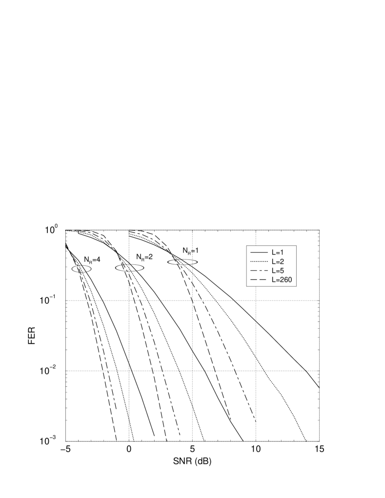
Figure 8: FER vs. SNR for P-STC obtained with the rate $1/2$, $64$ states convolutional encoder with generators $(133,171)_{8}$, $1\,bps/Hz$ BPSK, $n=2$ transmitting antennas and $m=1,2,4$ receiving antennas in BFC for various $L$.

In Fig. 8 the FER for a BPSK modulated P-STC obtained with the de-facto standard $64$ states convolutional encoder with octal generators $(133,171)_{8}$ is shown, assuming a BFC. In particular, $n=2$ transmitting antennas and $m=1,2,4$ receiving antennas are considered for various fading rates given by $L=1,2,5,260$ fading levels per codeword with $N=130$. Note that even with this not-optimized choice of the generators, P-STC are able to reach the maximum achievable spatial diversity; in particular for $L=1$ (i.e., quasi-static fading channel, meaning absence of time diversity), the diversity order is given by the product $n\cdot m$. For $L$ greater than $1$, thus in the presence of available time-diversity, the achieved diversity order increases, depending also on the number of states. For MIMO(2,2) P-STC, typical values of interest for the FER (i.e., in the order of $10^{-2}$) can be reached with $E_{b}/N_{0}$ per receiving antenna element of about $6$ dB (quasi-static channel), $3.8$ dB ($L=2$), $2.5$ dB ($L=5$) and $2$ dB (fully-interleaved case), whereas with $4$ receiving antennas the required SNR decreases to $0.2$ dB, $-1.1$ dB, $-1.6$ dB and $-2.1$ dB, respectively.

The low complexity of the P-STC architecture makes also feasible the use of a larger number of transmitting antennas. As an example, the case of $n=4$ is shown in Fig. 9 for quasi-static Rayleigh fading, $N=130$ and $m=1,2,4$. Here, the convolutional encoder with optimal AWGN generators $(135,135,147,163)_{8}$ is adopted [2]. Note that the case MIMO(4,2) achieves FER equal to $10^{-2}$ at $4.2$ dB, that is greater than the $0.2$ dB of the case MIMO(2,4) seen before; this is due to both the different power repartition on transmitting antennas and power combining at receiving antennas as well as the different code-rate.

Similarly, by using the generators for CC over AWGN it is possible to design $n$-P-STC for QPSK ($2$ bps/Hz) by using the rate $2/2n$ convolutional codes.

Let us now consider the search for optimum generators (in the sense defined in section VI). In Tab. I we report, for the quasi-static fading channel and QPSK, the characteristic parameters and performance of the best generators for the $(4,2,2)2$-P-STC, compared with the code proposed in [8] . Note that all codes achieve the available diversity $n\cdot m$, but with different performance factors $\tilde{F}_{\min}(m)/N$. It is remarkable that the ratio between performance factors is almost the same as the ratio of the simulated FERs. Moreover, even at SNR of $15$ dB, the asymptotic bound is sufficiently close to FER. Note also that the performance factor evaluated by fixing a reference codeword (${F}_{\min}(\underline{c}_{0},m)/N$) provides a slightly different ranking of generators, giving as best code the generator $(06,13,11,16)_{8}$. This code is not the best according to $\tilde{F}_{\text{min}}(m)$ (that would give $(05,11,06,16)_{8}$), but is very close to it terms of performance factor and the best in terms of FER. As will be clarified in the following, we checked that there are $11$ codes out of $2^{16}$ behaving as the first and $47$ behaving as the second, meaning that there is not a single best code but several codes that perform similarly.

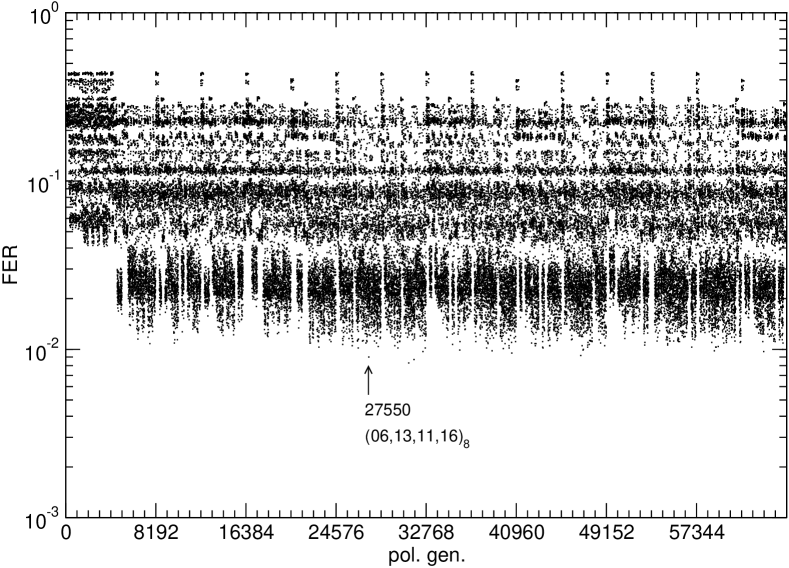
Figure 10: Exhaustive search for MIMO(2,2) P-STC in terms of FER: QPSK, quasi-static fading channel ($L=1$), $E_{b}/N_{0}=9$dB.

This fact suggests us to carefully investigate the performance differences among generators through exhaustive simulations. Thus, we performed an exhaustive simulation for all possible 4 states $n=2,m=2$ P-STC in terms of FER for QPSK in quasi-static fading channel, with $E_{b}/N_{0}=9$ dB. In Fig. 10 we report the FER for all $4$-states P-STC obtained through $2/4$ convolutional encoders (i.e., $2^{16}$ generators that are ordered in abscissa). A remarkable outcome is that also for P-STC it is verified a phenomenon similar to what already discussed in [24] for convolutional codes in BFC: non-catastrophic codes can be divided in few classes, with almost the same performance for codes in the same class. Note that within the class of codes providing the best performance, there is the one obtained through our searching methodology, that gives a FER of about $0.01$. Even for this simple case of $4$ states generators, the exhaustive search by simulation required one entire week on a Pentium 4 personal computer, whereas with our code searching algorithm we saved about two order of magnitude in time. An exhaustive search for a larger number of states is impractical, while our search algorithm works still well, emphasizing the importance of algorithmic methods.

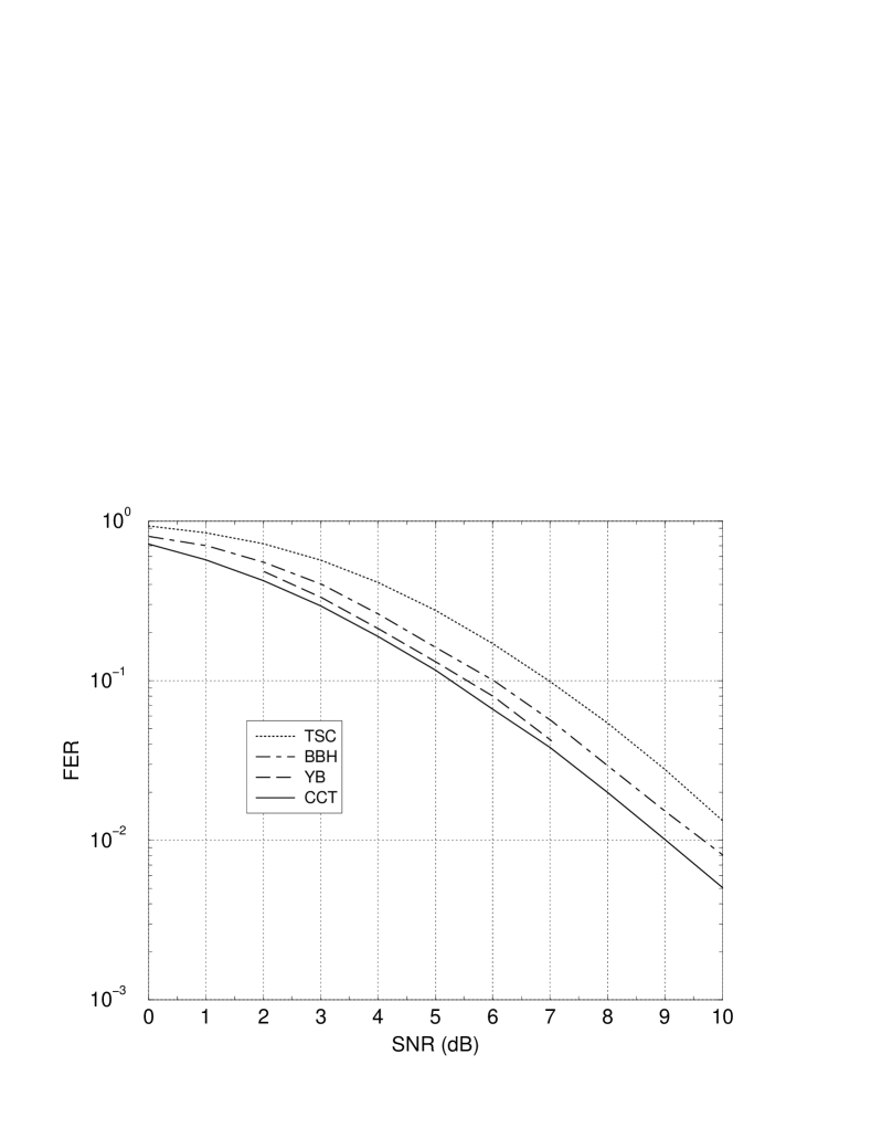
Figure 11: Comparison of our $4$ states QPSK MIMO(2,2), $2bps/Hz$, P-STC (continuous line) and previously known space-time codes. TSC: [8], BBH: [12], and YB: [14], quasi-static fading channel.

Hence, it is important to note that the pragmatic structure is not only interesting from the implementation point of view, but it also provides interesting performance, that, in all cases we investigated, outperformed the previously known STCs. In order to make the comparison between P-STC and STC possible, in the following numerical results we assume $N=130$ [8, 12, 14]. As an example, the performance of our best MIMO(2,2) QPSK (4,2,2) 2-P-STC (with generators $(06,13,11,16)_{8}$) is compared in Fig. 11 with other STC known in the literature for quasi-static channel [8, 12, 14]. These results show that out P-STC outperform previously known STC.

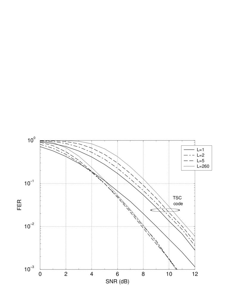
Figure 12: Comparison of our $4$ states QPSK MIMO(2,2), $2bps/Hz$, P-STC and the STC in [8] (TSC) for different fading rates.

Moreover, the proposed code search methodology also enables to find P-STC for various fading rates, that is, for various values of the parameter $L$. As an example, in the case of MIMO(2,2) QPSK (4,2,2) 2-P-STC, we obtain that the best generator is $(05,06,13,17)_{8}$ when $L\geq 2$, as shown in Fig. 12 for $L=1,2,5$, and $260$. At the author knowledge no other results for the BFC are present in the literature, so we compare our codes with the original STC in [8] even if the latter was designed for the quasi-static case. Note that with only $4$ states codes are not able to exploit all available time diversity, but the proposed codes already achieve the available spatial diversity.

Then, we investigate the impact of the number of states on the performance of MIMO(2,1) P-STC with BPSK in quasi-static fading channel. In Tab. II we report best codes obtained through the search algorithm for $2,4,8,16$ states, for which we indicate the achieved diversity, the performance factor and the FER. We also report the performance factor for AWGN optimal generators with the same number of states. Note that all codes achieve the maximum diversity, and that increasing the number of states does not produce relevant performance improvements. Moreover, on the quasi-static channel the error probability bound tends to become looser, especially when the free distance of the convolutional code increases with respect to the achieved diversity.

The behavior is different in BFC with time diversity available. This case is illustrated in Tab. III for $L=8$, where it is shown that increasing the number of states results in a larger diversity. Note also that the optimum P-STC are able to achieve a diversity equal to that achieved by using the optimal generators for the AWGN channel, and that are not able to reach the diversity achievable on the RBFC with $nL$ fading levels per codeword. This means that convolutional codes are more capable to collect time diversity than spatial diversity.

Finally, we report in Tabs. IV, V, and VI the optimum generators obtained through the search algorithm for $n=2,3,4,$ respectively, with BPSK and QPSK modulations, and for different number of states. The corresponding performance factors are also reported. It is worth noting that, although the codes are not geometrically uniform, in most cases the code search based on the ST-GTF with a fixed reference codeword leads to the same code as the search over all possible transmitted codewords, or to a code with similar performance.

VIII Conclusions

In this paper we investigated the feasibility of a pragmatic approach to space-time codes, where common convolutional encoders and decoders are used, with suitably defined branch metrics.

We extended to pragmatic space-time codes the concept of generalized transfer function for convolutional codes in block fading channels, that results in the possibility to rank different codes with an efficient algorithm, based on the asymptotic error probability union bound. A search methodology to obtain optimum generators for different fading rates has then been proposed.

It has been shown that P-STC achieve better performance compared to previously known STC and that they are suitable for systems with different spectral efficiencies, number of antennas and fading rates, and are therefore a valuable choice both in terms of implementation complexity and performance.

Appendix

An example of computation of the ST-GTF for P-STC is reported here. We consider a (2,1,2) 2-PSTC used with $m=1$ receiving antenna over a quasi-static BFC and obtained from a $1/2$ convolutional code with generators $(1,3)_{8}$ and BPSK modulation format. These generators are the best for two-states CC in AWGN, with free distance 3; when used to build a P-STC we checked that this choice of generators produces the second best code in quasi-static fading channels, achieving diversity 2, i.e. the maximum available diversity. This code has been chosen since simple enough to allow the evaluation of $time-0$ ST-GTF, $T_{M0}({\bf D})$, using standard algorithm on the modified error state diagram. The two-states trellis is depicted in Fig. 7 (up-left).

The associated possible output symbols $[c_{1};c_{2}]$ and $[g_{1};g_{2}]$ are in the set $\{X_{0},X_{1},X_{2},X_{3}\}$ with $X_{0}=[-1;-1]$, $X_{1}=[-1;1]$, $X_{2}=[1;-1]$ and $X_{3}=[1;1]$. Thus, the matrix ${\bf A}(\underline{c},\underline{g})$ is in the set $\{{\bf a,b,c,d,e}\}$ with

$${\bf a}=\begin{pmatrix}0&0\\ 0&0\end{pmatrix}\qquad{\bf b}=\begin{pmatrix}4&0\\ 0&0\end{pmatrix}\qquad{\bf c}=\begin{pmatrix}0&0\\ 0&4\end{pmatrix}\qquad{\bf d}=\begin{pmatrix}4&4\\ 4&4\end{pmatrix}\qquad{\bf e}=\begin{pmatrix}4&-4\\ -4&4\end{pmatrix}.$$

The error state diagram modified by splitting the all-zero state with different labeling $\hat{0}$ and $\dot{0}$ is given in Fig. 7 (up-right). Thus, by following the steps in Sec.V-A we rewrite the error state diagram for quasi-static fading channel as in Fig. 7 (down-left) where

$${\bf\alpha}(D)=1/2\begin{pmatrix}D^{\bf c}&D^{\bf c}\\ D^{\bf c}&D^{\bf c}\end{pmatrix}\qquad{\bf\beta}(D)=1/2\begin{pmatrix}D^{\bf b}&D^{\bf b}\\ D^{\bf b}&D^{\bf b}\end{pmatrix}\qquad{\bf\gamma}(D)=1/2\begin{pmatrix}D^{\bf d}&D^{\bf e}\\ D^{\bf d}&D^{\bf e}\end{pmatrix}.$$

The corresponding ST-GTF results in

$$\begin{cases}{\bf Q}_{S}^{T}(D)={\bf U}_{0}^{T}{\bf\alpha}(D)+{\bf Q}_{S}^{T}{\bf\beta}(D)&\\ {\bf Q}_{\dot{0}}^{T}(D)={\bf Q}_{S}^{T}(D){\bf\gamma}(D)&\\ \end{cases}\Rightarrow\begin{cases}{\bf Q}_{S}^{T}(D)={\bf U}_{0}^{T}{\bf\alpha}(D)\left({\bf I}-{\bf\beta}(D)\right)^{-1}&\\ {\bf Q}_{\dot{0}}^{T}(D)={\bf U}_{0}^{T}{\bf\alpha}(D)\left({\bf I}-{\bf\beta}(D)\right)^{-1}{\bf\gamma}(D)&\\ \end{cases}$$ (33)

giving

$$T_{M0}(D)={\bf Q}_{\dot{0}}^{T}(D){\bf U}_{0}=\frac{1}{4}[D^{\bf c}\ D^{\bf c}]\left({\bf I}-{\bf\beta}(D)\right)^{-1}[D^{\bf d}\ D^{\bf d}]^{T}=\frac{D^{{\bf c}+{\bf d}}}{1-D^{\bf b}}\,,$$ (34)

which can also be expanded in

$$T_{M0}(D) = D^{{\bf c}+{\bf d}}(1+D^{b}/(1-D^{\bf b}))=D^{{\bf c}+{\bf d}}+D^{{\bf c}+{\bf d}+{\bf b}}(1+D^{\bf b}/(1-D^{\bf b}))=\ldots$$ (35)

$$= D^{{\bf c}+{\bf d}}+D^{{\bf c}+{\bf d}+{\bf b}}+D^{{\bf c}+{\bf d}+2{\bf b}}+\ldots\,.$$

Therefore, to obtain the ST-GTF of the code we need to compute the eigenvalues of matrices of the form ${\bf c}+{\bf d}+i{\bf b}$ with $i\geq 0$ integer, and

$$\mathcal{T}\left[T_{M0}(D)\right]=\sum_{i=0}^{+\infty}d_{1}^{\lambda_{i1}}d_{2}^{\lambda_{i2}}\,,$$ (36)

where $\lambda_{i1}$ and $\lambda_{i2}$ are the two eigenvalues of ${\bf c}+{\bf d}+i{\bf b}$ (e.g., $\lambda_{01}=\lambda_{02}=6\pm\sqrt{20}$) while their product is simply $\lambda_{i1}\lambda_{i2}=2i+1$. Then, we obtain $\tilde{\eta}_{\text{min}}=2$ and $\tilde{F}_{\text{min}}(1)\approx(N/16)(1+1/3+1/5+\ldots)$. It is interesting to note that both ${\bf\alpha}(D)$ and ${\bf\beta}(D)$ have equal elements, that ${\bf e}$ and ${\bf e}$ can be interchanged without altering the eigenvalues, and thus the ST-GTF does not depend on the particular reference sequence. Therefore this code is geometrically uniform even at the output of the channel. As check we can evaluate $T_{0}(D)$ for the all-zero reference codeword $\underline{c}=\underline{c}_{0}$ by exploiting the error state diagram with scalar labels; to this aim it is sufficient to replace $\alpha(D)=D^{\bf c}$, $\beta(D)=D^{\bf b}$ and $\gamma(D)=D^{\bf d}$, so obtaining

$$T_{0}(D)=\alpha(D)(1-\beta(D))^{-1}\gamma(D)=\frac{D^{{\bf c}+{\bf d}}}{1-D^{\bf b}}\,,$$ (37)

which is equal to $T_{M0}(D)$ in (34).

To evaluate the ST-GTF of the P-STC in a BFC with $L=2$ and periodical interleaving, i.e., $\mathbf{\Delta}=\left(D_{1}D_{2}D_{1}D_{2}\ldots\right)$, we can extend the error state diagram by replacing the state $S$ with two states $S_{1}$ and $S_{2}$, thus obtaining transitions $\hat{0}\rightarrow S_{1}$ with output $D_{1}^{\bf c}$, $S_{1}\rightarrow S_{2}$ with output $D_{2}^{\bf b}$, $S_{2}\rightarrow S_{1}$ with output $D_{1}^{\bf b}$, $S_{1}\rightarrow\dot{0}$ with output $D_{2}^{\bf d}$ and $S_{2}\rightarrow\dot{0}$ with output $D_{1}^{\bf d}$ (see Fig. 7 down-right). The ST-GTF is then

$$\begin{cases}Q_{S_{1}}(D_{1},D_{2})=D_{1}^{\bf c}+Q_{S_{2}}(D_{1},D_{2})D_{1}^{\bf b}&\\ Q_{S_{2}}(D_{1},D_{2})=Q_{S_{1}}(D_{1},D_{2})D_{2}^{\bf b}&\\ Q_{\dot{0}}(D_{1},D_{2})=Q_{S_{1}}(D_{1},D_{2})D_{2}^{\bf d}+Q_{S_{2}}(D_{1},D_{2})D_{1}^{\bf d}&\\ \end{cases}\Rightarrow\begin{cases}Q_{S_{1}}(D_{1},D_{2})=\frac{D_{1}^{\bf c}}{1-D_{1}^{\bf b}D_{2}^{\bf b}}&\\ Q_{S_{2}}(D_{1},D_{2})=\frac{D_{1}^{\bf c}D_{2}^{b}}{1-D_{1}^{\bf b}D_{2}^{\bf b}}&\\ Q_{\dot{0}}(D_{1},D_{2})=\frac{D_{1}^{\bf c}D_{2}^{\bf b}+D_{1}^{{\bf c}+{\bf d}}D_{2}^{\bf b}}{1-D_{1}^{\bf b}D_{2}^{\bf b}}&\\ \end{cases}$$ (38)

and after expansion

$$T_{0}(D_{1},D_{2})=T_{M0}(D_{1},D_{2})=D_{1}^{\bf c}D_{2}^{d}+D_{1}^{{\bf c}+{\bf d}}D_{2}^{\bf b}+D_{1}^{{\bf c}+{\bf b}}D_{2}^{{\bf d}+{\bf b}}+D_{1}^{{\bf c}+{\bf d}+{\bf b}}D_{2}^{2{\bf b}}+\ldots\,,$$ (39)

in which only $D_{1}^{\bf c}D_{2}^{\bf d}$ has two terms with rank $1$. Therefore $\mathcal{T}[D_{1}^{\bf c}D_{2}^{\bf d}]=d_{11}^{1}d_{21}^{1}$ implying $\tilde{\eta}_{\text{min}}=2$ and $\tilde{F}_{\text{min}}(1)\approx N/16$.

Figure 1: Equivalent low-pass scheme for space-time codes.

Figure 2: Equivalent low-pass scheme for the proposed pragmatic space-time codes.

Figure 3: Example of $1\ bps/Hz$ pragmatic space-time encoder for $n=2$ transmitting antennas and BPSK modulation, obtained with a rate $1/2$ convolutional encoder with $4$ states and generator polynomials $(5,7)_{8}$.

Figure 4: Trellis for the pragmatic space-time code of Fig. 3. On each branch the first is the input bit, followed by the two output antipodal symbols.

Figure 5: Example of $2\ bps/Hz$ pragmatic space-time encoder for $n=2$ transmitting antennas and QPSK modulation, obtained with a rate $2/4$ convolutional encoder with $4$ states and generator polynomials $(06,13,11,16)_{8}$.

Figure 6: Receiver structure for the proposed pragmatic space-time codes. In the figure the Viterbi decoder is the usual for the convolutional code adopted in transmission, with the only change that the metric on a generic branch is, for $n=2$, $\sum_{s=1}^{m}|r_{s}^{(t)}-\sqrt{E_{s}}\left(h^{(t)}_{1,s}\widetilde{c_{1}}+h^{(t)}_{2,s}\widetilde{c_{2}}\right)|^{2}$, being $\widetilde{c_{1}},\widetilde{c_{2}}$ the two symbols associated to the branch.

Figure 7: Trellis and state diagrams for the P-STC investigated in appendix.

Figure 9: FER vs. SNR for P-STC obtained with $1/4$ convolutional encoder, $64$ states, BPSK, $1\ bps/Hz$, $4$ transmitting antennas and $1,2,4$ receiving antennas in quasi-static Rayleigh fading channel.

TABLE I: Comparison of rate $2/4$ P-STC with QPSK, $n=m=2$, $\mu=2$ on BFC with $L=1$, $E_{b}/N_{0}=15dB$ and $N=130$. The performance factor is truncated with $\delta_{H}=9$. The first two codes are the best produced by the search (there are 12 first-class codes with almost the same behavior, and 48 second-class codes). The third code is the code proposed in [8].

Generators	$d_{f}$	$\tilde{\eta}_{min}m$	$\tilde{F}_{\min}(2)/N$	${F}_{\min}(\underline{c}_{0},2)/N$	$\tilde{P}_{w\infty}$	$FER$
$(06,13,11,16)_{8}$	4	4	0.076	0.048	$3.5\ 10^{-4}$	$9.3\ 10^{-5}$
$(05,11,06,16)_{8}$	4	4	0.073	0.092	$3.4\ 10^{-4}$	$1.0\ 10^{-4}$
$(01,02,04,10)_{8}$	2	4	0.125	0.125	$5.7\ 10^{-4}$	$2.4\ 10^{-4}$

TABLE II: Optimum rate $1/2$ P-STC with BPSK, $n=2$, $m=1$ on BFC with $L=1$. Parameters with superscript ⁽¹⁾ refer to the codes obtained with best convolutional codes for AWGN channel. The performance factor is truncated with $\delta_{H}=2d_{f}^{(1)}-1$. Error performance refers to $E_{b}/N_{0}=20dB$ and $N=130$.

$\mu$	Generators	Generators(1)	$d_{f}$	$\tilde{\eta}_{min}$	$\tilde{F}_{\min}(1)/N$	$d_{f}^{(1)}$	$\tilde{F}_{\min}^{(1)}(1)/N$	$FER$	$FER^{(1)}$
2	$(1,2)_{8}$	$(1,3)_{8}$	2	2	0.083	3	0.096	$2.7\ 10^{-3}$	$3.2\ 10^{-3}$
3	$(3,4)_{8}$	$(5,7)_{8}$	3	2	0.151	5	0.191	$1.7\ 10^{-3}$	$1.8\ 10^{-3}$
4	$(13,15)_{8}$	$(15,17)_{8}$	6	2	0.217	6	0.359	$1.0\ 10^{-3}$	$1.3\ 10^{-3}$
5	$(23,31)_{8}$	$(23,35)_{8}$	6	2	0.372	7	0.79	$0.8\ 10^{-3}$	$0.9\ 10^{-3}$

TABLE III: Optimum rate 1/2 P-STC with BPSK, $n=2$, $m=1$ on BFC with $L=8$. Parameters with superscript ⁽¹⁾ refer to the codes obtained with best convolutional codes for AWGN channel. The performance factor is truncated with $\delta_{H}=2d_{f}^{(1)}-1$. $\tilde{\eta}_{min}^{(R\acs{BFC})}$ is the diversity achievable on the RBFC with $nL$ fading blocks [24]; the value of the Singleton bound is 9.

$\mu$	Generators	$\tilde{\eta}_{min}$	$\tilde{F}_{\min}(1)/N$	$\tilde{\eta}_{min}^{(1)}$	$\tilde{F}_{\min}^{(1)}(1)/N$	$\tilde{\eta}_{min}^{(R\acs{BFC})}$
2	(1,3)	2	0.031	2	0.031	4
3	(5,7)	3	0.0039	3	0.0039	5
4	(07,15)	4	9.8 $10^{-4}$	4	14.6 $10^{-4}$	6
5	(13,36)	5	3.7 $10^{-4}$	5	7.5 $10^{-4}$	7
6	(57,75)	6	2.3 $10^{-4}$	6	2.3 $10^{-4}$	8
7	(115,163)	6	2.3 $10^{-5}$	6	1.0 $10^{-4}$	8

TABLE IV: Optimum P-STC for a system with $n=2$, $m=1$ on BFC with $L=1$. Symbol $*$ indicates that the search based on ${F}_{\min}(\underline{c}_{0},m)$ leads to the same code as the full search.

n	k	$\mu$	h	Generators	$\tilde{\eta}_{min}$	$\tilde{F}_{\min}(1)/N$	${F}_{\min}(\underline{c}_{0},1)/N$	$\tilde{F}_{\min}(2)/N$
2	1	2	1	(1,2)	2	0.083	0.083 *	0.0048 *
2	1	3	1	(3,4)	2	0.15	0.16	0.017
2	1	4	1	(13,15)	2	0.22	0.27	0.011 *
4	1	2	2	(1,2,3,1)	2	0.082	0.087	0.003 *
4	1	3	2	(2,5,7,6)	2	0.12	0.14	0.0011 *
4	1	4	2	(11,15,17,13)	2	0.24	0.30	0.00083 *
4	2	2	2	(06,13,11,16)	2	1.37	1.29 *	0.073

TABLE V: Optimum P-STC for a system with $n=3$, $m=1$ on BFC with $L=1$. Symbol $*$ indicates that the search based on ${F}_{\min}(\underline{c}_{0},m)$ leads to the same code as the full search. N.E.=Not evaluated.

n	k	$\mu$	h	Generators	$\tilde{\eta}_{min}$	$\tilde{F}_{\min}(1)/N$	${F}_{\min}(\underline{c}_{0},1)/N$
3	1	2	1	(1,2,3)	2	0.026	0.021 *
3	1	3	1	(2,3,4)	3	0.030	0.033
3	1	4	1	(11,12,15)	3	0.033	0.044
6	1	2	2	(1,1,2,2,3,3)	2	0.027	0.021 *
6	1	3	2	(1,5,3,2,6,1)	3	0.017	0.019
6	2	2	2	(05,05,06,11,11,13)	2	N.E.	0.05

TABLE VI: Optimum P-STC for a system with $n=4$, $m=1$ on BFC with $L=1$. Symbol * indicates that the search based on ${F}_{\min}(\underline{c}_{0},m)$ leads to the same code as the full search. N.E.=Not evaluated.

n	k	$\mu$	h	Generators	$\tilde{\eta}_{min}$	$\tilde{F}_{\min}(1)/N$	${F}_{\min}(\underline{c}_{0},1)/N$
4	1	2	1	(1,1,2,3)	2	0.016	0.013 *
4	1	3	1	(1,3,5,7)	3	0.0045	0.0039
4	1	4	1	(03,05,11,16)	4	N.E.	0.0057

References

- [1] M. Schwarz, W. R. Bennett, and S. Stein, Communications Systems and Techniques, classic reissue ed. Piscataway, New Jersey, 08855-1331: IEEE Press, 1996.
- [2] J. G. Proakis, Digital Communications, 4th ed. New York, NY, 10020: McGraw-Hill, Inc., 2001.
- [3] J. H. Winters, “Smart antennas for wireless systems,” IEEE Pers. Commun. Mag., pp. 23–27, Feb. 1998.
- [4] S. M. Alamouti, “A simple transmit diversity technique for wireless communications,” IEEE J. Select. Areas Commun., vol. 16, no. 8, pp. 1451–1458, Oct. 1998.
- [5] A.Narula, M.D.Trott, and G.W.Wornell, “Performance limits of coded diversity methods for transmitter antenna arrays,” IEEE Trans. Inform. Theory, vol. 45, no. 7, pp. 2418–2433, Nov. 1999.
- [6] A.Wittneben, “A new bandwidth efficient transmit antenna modulation diversity scheme for linear digital modulation,” Proc. IEEE Int. Conf. on Comm., pp. 1630–1634, June 1993, Geneve.
- [7] J.-C.Guey, M.P.Fitz, M.R.Bell, and W.-Y. Kuo, “Signal design for transmitter diversity wireless communication systems over rayleigh fading channels,” Proc. 46th Annual Int. Veh. Technol. Conf., pp. 136–140, Sept. 1996, atlanta, GA.
- [8] V. Tarokh, N. Seshadri, and A. R. Calderbank, “Space-time codes for high data rate wireless communication: performance criterion and code construction,” IEEE Trans. Inform. Theory, vol. 44, no. 2, pp. 744–765, Mar. 1998.
- [9] V. Tarokh, A. F. Naguib, N. Seshadri, and A. R. Calderbank, “Space-time codes for high data rate wireless communication: performance criteria in the presence of channel estimation errors, mobility, and multiple paths,” IEEE Trans. Commun., vol. 47, no. 2, pp. 199–207, Feb. 1999.
- [10] B. Vucetic and J. Yuan, Space-Time Coding. John Wiley & Sons Ltd, The Atrium, Southern Gate, Chichester, West Sussex PO19 8SQ, England: Wiley, 2003.
- [11] H. Jafarkhani, Space-Time Coding Theory and Practice. Cambridge University Press: Cambridge, 2005.
- [12] S.Baro, G.Bauch, and A.Hansmann, “Improved codes for space-time trellis-coded modulation,” IEEE Commun. Lett., vol. 4, no. 1, pp. 20–22, Jan. 2000.
- [13] Z. Chen, J. Yuan, and B. Vucetic, “Improved space-time trellis coded modulation scheme on slow Rayleigh fading channels,” Electron. Lett., vol. 37, no. 7, pp. 440–441, Mar. 2001.
- [14] Q.Yan and R.S.Blum, “Improved space-time convolutional codes for quasi-static slow fading channels,” IEEE Trans. on Wireless Commun., vol. 1, no. 4, pp. 563–571, Oct. 2002.
- [15] A.R.Hammons and H. El Gamal, “On the theory of space-time codes for psk modulation,” IEEE Trans. Inform. Theory, vol. 46, no. 2, pp. 524–542, Mar. 2000.
- [16] H. El Gamal and A.R.Hammons, “On the design of algebraic space-time codes for MIMO block-fading channels,” IEEE Trans. Inform. Theory, vol. 49, no. 1, pp. 151–163, Jan. 2003.
- [17] R.J.McEliece and W.E.Stark, “Channels with block interference,” IEEE Trans. Inform. Theory, vol. 30, no. 1, pp. 44–53, Jan. 1984.
- [18] M. Chiani, “Error probability for block codes over channels with block interference,” IEEE Trans. Inform. Theory, vol. 44, no. 7, pp. 2998–3008, Nov. 1998.
- [19] E. Malkamaki and H.Leib, “Coded diversity on block-fading channels,” IEEE Trans. Inform. Theory, vol. 45, no. 2, pp. 771–781, Mar. 1999.
- [20] M. Chiani, A. Conti, and V. Tralli, “A pragmatic approach to space-time coding,” in Proc. IEEE Int. Conf. on Commun., vol. 9, Helsinki, FI, June 2001, pp. 2794 – 2799.
- [21] A.J.Viterbi, J.K.Wolf, E.Zehavi, and R.Padovani, “A pragmatic approach to trellis-coded modulation,” IEEE Commun. Mag., vol. 27, no. 7, pp. 11–19, July 1989.
- [22] J. H. Winters, J. Salz, and R. D. Gitlin, “The impact of antenna diversity on the capacity of wireless communication system,” IEEE Trans. Commun., vol. 42, no. 2/3/4, pp. 1740–1751, Feb./Mar./Apr. 1994.
- [23] M. Chiani, A. Conti, and V. Tralli, “Bit-interleaved pragmatic space-time codes: design and code construction,” in Proc. IEEE Global Telecomm. Conf., vol. 2, Taipei, TW, Nov. 2002, pp. 1940–1944.
- [24] ——, “Further results on convolutional code search for block-fading channels,” IEEE Trans. Inform. Theory, vol. 50, no. 6, pp. 1312–1318, June 2004.
- [25] G.Caire and E.Viterbo, “Upper bound on the frame error probability of terminated trellis codes,” IEEE Commun. Lett., vol. 2, no. 1, pp. 2–4, Jan. 1998.
- [26] C. Schlegel, “Evaluating distance spectra and performance bounds of trellis codes on channels with intersymbol interference,” IEEE Trans. Inform. Theory, vol. 37, no. 3, pp. 627–634, May 1991.
- [27] S. Benedetto and E. Biglieri, Principles of Digital Transmission with Wireless Applications. Kluwer Academic, 1998.
- [28] M. Chiani, A. Conti, and V. Tralli, “Further results on convolutional code search for block-fading channels,” IEEE Trans. Inform. Theory, vol. 50, no. 6, pp. 1312 – 1318, June 2004.
- [29] M. Chiani, D. Dardari, and M. K. Simon, “New exponential bounds and approximations for the computation of error probability in fading channels,” IEEE Trans. Wireless Commun., vol. 2, no. 4, pp. 840 – 845, July 2003.
- [30] G. D. Forney Jr., “Geometrically uniform codes,” IEEE Trans. Inform. Theory, vol. 37, no. 5, pp. 1241–1260, Sept. 1991.
- [31] Z. Yan and D. M. Ionescu, “Geometrical uniformity of a class of space-time trellis codes,” IEEE Trans. Inform. Theory, vol. 50, no. 12, pp. 3343–3347, Dec. 2004.
- [32] E. Malkamaki and H.Leib, “Evaluating the performance of convolutional codes over block fading channels,” IEEE Trans. Inform. Theory, vol. 45, no. 5, pp. 1643–1646, July 1999.
- [33] R.A.Horn and C.R.Johnson, Matrix Analysis. UK: Cambridge University Press, 1999.