Adaptive Methods for Linear Programming Decoding

Abstract

Detectability of failures of linear programming (LP) decoding and the potential for improvement by adding new constraints motivate the use of an adaptive approach in selecting the constraints for the underlying LP problem. In this paper, we make a first step in studying this method, and show that it can significantly reduce the complexity of the problem, which was originally exponential in the maximum check-node degree. We further show that adaptively adding new constraints, e.g. by combining parity checks, can provide large gains in the performance.

I Introduction

Linear programming (LP) decoding, as an approximation to maximum-likelihood (ML) decoding, was proposed by Feldman et al. [1]. Many observations suggest similarities between the performance of LP and iterative message-passing decoding methods. For example, we know that the existence of low-weight pseudocodewords degrades the performance of both types of decoders [1], [2], [3]. Therefore, it is reasonable to try to exploit the simpler geometrical structure of LP decoding to make predictions about the performance of message-passing decoding algorithms.

On the other hand, there are differences between these two decoding approaches. For instance, given an LDPC code, we know that adding redundant parity checks that are satisfied by all the codewords can not degrade the performance of LP decoding, while with message-passing algorithms, these parity checks may have a negative effect by introducing short cycles in the corresponding Tanner graph. This property of LP decoding allows performance improvement by tightening the relaxation. Another characteristic of LP decoding – the ML certificate property – is that its failure to find an ML codeword is always detectable. More specifically, the decoder always gives either an ML codeword or a nonintegral pseudocodeword as the solution.

These two properties motivate the use of an adaptive approach in LP decoding which can be summarized as follows: Given a set of constraints that describe a code, start the LP decoding with a few of them, then sequentially and adaptively add more of the constraints to the problem until either an ML codeword is found or no further “useful” constraint exists. The goal of this paper is to explore the potential of this idea for improving the performance of LP decoding.

We show that by incorporating adaptivity into the LP decoding procedure, we can achieve with a small number of constraints an error-rate performance comparable to that obtained when standard LP decoding is applied to a relaxation defined by a much larger number of constraints. In particular, we observe that while the number of constraints per check node required for convergence of LP decoding is exponential in the check node degrees, the adaptive method generally converges with a (small) constant number of constraints that does not appear to be dependent upon the underlying code s degree distribution. This property makes it feasible to apply LP decoding to higher-density graph codes.

Along the way, we prove several general properties of LP relaxations of ML decoding that shed light upon the performance of LP and iterative decoding algorithms.

The rest of this paper is organized as follows. In Section II, we review Feldman’s LP decoding. In Section III, we introduce and analyze an adaptive algorithm to solve the original LP problem more efficiently. In Section IV, we study how adaptively imposing additional constraints can improve the LP decoder performance. Section V concludes the paper.

II LP Relaxation of ML Decoding

Consider a binary linear code $\mathscr{C}$ of length $n$. If a codeword $\underline{y}\in\mathscr{C}$ is transmitted through a memoryless binary-input output-symmetric (MBIOS) channel, the ML codeword given the received vector $\underline{r}\in\mathbb{R}^{n}$ is the solution to the optimization problem

minimize $$\underline{\gamma}^{T}\underline{x}$$

subject to $$\underline{x}\in\mathscr{C},$$ (1)

where $\underline{\gamma}$ is the vector of log-likelihood ratios defined as

$$\gamma_{i}=\log\left(\frac{\Pr(r_{i}|y_{i}=0)}{\Pr(r_{i}|y_{i}=1)}\right).$$ (2)

As an approximation to ML decoding, Feldman et al. proposed a relaxed version of this problem by first considering the convex hull of the local codewords defined by each row of the parity-check matrix, and then intersecting them to obtain what is called the fundamental polytope, $\mathscr{P}$, by Koetter et al. [3]. This polytope has a number of integral and nonintegral vertices, but the integral vertices exactly correspond to the codewords of $\mathscr{C}$. Therefore, whenever LP decoding gives an integral solution, it is guaranteed to be an ML codeword.

In Feldman’s relaxation of the decoding problem, constraints are derived from a parity-check matrix as follows. For each row $j=1,\ldots,m$ of the parity-check matrix, define the neighborhood set $N(j)\subset\{1,2,\ldots,n\}$ of the corresponding check node in the Tanner graph to be the variable nodes that are directly connected to it. (For convenience, we often identify check nodes and variable nodes with their respective index sets $j=1,\ldots,m$ and $i=1,\ldots,n$.) Then, for $j=1,\ldots,m$ the LP relaxation includes all of the following constraints:

$$\sum_{i\in V}x_{i}-\sum_{i\in N(j)\backslash V}x_{i}\leq|V|-1,\ \ \forall\ V\subset N(j)\ \textrm{such that}\ |V|\ \textrm{is odd}.$$ (3)

Throughout the paper, we refer to the constraints of this form as parity-check constraints. In addition, for any element $x_{i}$ of the optimization variable, $\underline{x}$, the constraint that $0\leq x_{i}\leq 1$ is also added.

III Adaptive LP Decoding

As any odd-sized subset $V$ of the neighborhood $N$ of each check node introduces a unique parity-check constraint, there are $2^{d_{c}-1}$ constraints corresponding to each check node of degree $d_{c}$. Therefore, the total number of constraints and hence, the complexity of the problem, is exponential in terms of the maximum check node degree, $d_{c}^{max}$. This becomes more significant in a high density code where $d_{c}^{max}$ increases with the code length, $n$. In this section, we show that Feldman s LP relaxation has some properties that allow us to solve the optimization problem by using a much smaller number of constraints.

III-A Properties of the Relaxation Constraints

Definition 1

Given a constraint of the form

$$\underline{a}_{i}^{T}\underline{x}\leq b_{i},$$ (4)

and a vector $\underline{x}_{0}\in\mathbb{R}^{n}$, we call (4) an active constraint at $\underline{x}_{0}$ if

$$\underline{a}_{i}^{T}\underline{x}_{0}=b_{i},$$ (5)

and a violated constraint or, equivalently, a cut at $\underline{x}_{0}$ if

$$\underline{a}_{i}^{T}\underline{x}_{0}>b_{i}.$$ (6)

A constraint that generates a cut at point $\underline{x}$ corresponds to a subset $V\subset N$ of odd cardinality such that

$$\sum_{i\in V}x_{i}-\sum_{i\in N\backslash V}x_{i}>|V|-1.$$ (7)

This condition implies that

$$|V|-1<\sum_{i\in V}x_{i}\leq|V|$$ (8)

and

$$0\leq\sum_{i\in N\backslash V}\!\!\!x_{i}<x_{\ell},\ \forall\ell\in V.$$ (9)

The following theorem reveals a special property of the constraints of the LP decoding problem.

Theorem 1

At any given point $\underline{x}\in[0,1]^{n}$, at most one of the constraints introduced by each check node can be a cut.

Proof:

Consider a check node with neighborhood $N\subset\{1,2,\ldots,n\}$ and two subsets $V_{1}\subset N$ and $V_{2}\subset N$ of odd sizes $\left|V_{1}\right|$ and $\left|V_{2}\right|$, respectively, that each introduce a cut at point $\underline{x}$. We prove the theorem by showing that these two cuts must be identical, i.e. $V_{1}=V_{2}$.

Partition $N$ into four disjoint subsets $S=V_{1}\cap V_{2}$, $\overline{V}_{1}=V_{1}\backslash V_{2}$, $\overline{V}_{2}=V_{2}\backslash V_{1}$, and $\overline{N}=N\backslash(V_{1}\cup V_{2})$. Now we can write the two corresponding constraints as

$$\sum_{i\in S}x_{i}+\sum_{i\in\overline{V}_{1}}x_{i}-\sum_{i\in\overline{V}_{2}}x_{i}-\sum_{i\in\overline{N}}x_{i}>|S|+\left|\overline{V}_{1}\right|-1,$$ (10)

and

$$\sum_{i\in S}x_{i}+\sum_{i\in\overline{V}_{2}}x_{i}-\sum_{i\in\overline{V}_{1}}x_{i}-\sum_{i\in\overline{N}}x_{i}>|S|+\left|\overline{V}_{2}\right|-1.$$ (11)

Now, we add the two inequalities and divide both sides by 2 to get

$$\sum_{i\in S}x_{i}-\sum_{i\in\overline{N}}x_{i}>|S|+\frac{\left|\overline{V}_{1}\right|+\left|\overline{V}_{2}\right|}{2}-1.$$ (12)

Since $x_{i}\in[0,1]$ for every $i$, the left-hand side is less than or equal to $|S|$. Hence, for the right-hand side, we should have

$$|S|+\frac{\left|\overline{V}_{1}\right|+\left|\overline{V}_{2}\right|}{2}-1<|S|,$$ (13)

which yields

$$\left|\overline{V}_{1}\right|+\left|\overline{V}_{2}\right|<2.$$ (14)

Knowing that $\left|V_{1}\right|=\left|S\right|+\left|\overline{V}_{1}\right|$ and $\left|V_{2}\right|=\left|S\right|+\left|\overline{V}_{2}\right|$ are both positive odd numbers, we conclude that their difference, $\left|V_{1}\right|-\left|V_{2}\right|=\left|\overline{V}_{1}\right|-\left|\overline{V}_{2}\right|$ is an even number. Therefore $\left|\overline{V}_{1}\right|+\left|\overline{V}_{2}\right|$ is an even number, as well. Hence, (14) can hold only if $\left|\overline{V}_{1}\right|+\left|\overline{V}_{2}\right|=0$, which means that $\left|\overline{V}_{1}\right|=\left|\overline{V}_{2}\right|=0$. It follows that $V_{1}$ and $V_{2}$ are identical. ∎

Given an $(n,k)$ linear code with $m=n-k$ parity checks, a natural question is how we can find all the cuts defined by the LP relaxation at any given point $\underline{x}\in\mathbb{R}^{n}$. Referring to (9), we see that for any check node and any odd-sized subset $V$ of its neighborhood $N$ that introduces a cut, the variable nodes in $V$ have the largest values among all of the nodes in $N$. Therefore, sorting the elements of $\underline{x}$ can simplify the process of searching for a cut. This observation is reflected in Algorithm 1 below.

Consider a check node with neighborhood $N$. Without loss of generality, assume that variable nodes in $N$ have indices $1,2,\ldots,|N|$, and that their values satisfy $x_{1}\geq x_{2}\geq\cdots\geq x_{|N|}$. The following algorithm provides an efficient way to find the unique cut generated by this check node at $\underline{x}$, if a cut exists.

Algorithm 1

Step 1: Set $v=1$, $V=\{1\}$ and $V^{c}\triangleq N\backslash V=\{2,3,\ldots,|N|\}$.

Step 2: Check the constraint (3). If it is violated, we have found the cut. Exit.

Step 3: Set $v=v+2$. If $v\leq|N|$, move $x_{v-1}$ and $x_{v}$ (the two largest members of $V^{c}$) from $V^{c}$ to $V$

Step 4: If $v\leq|N|$ and (8) is satisfied, go to Step 2; otherwise, the check node does not provide a cut at $x$.

Note that the failure of condition (8) provides a definitive termination criterion for the algorithm when no cut exists. If redundant calculations are avoided in calculating the sums in (3), this algorithm can find the cut generated by the check node, if it exists, in $O(d_{c})$ time, where $d_{c}=|N|$ is the degree of the check node. Repeating the procedure for each check node, and considering $O(n\log n)$ complexity for sorting $\underline{x}$, the time required to find all the cuts at point $\underline{x}$ becomes $O(md_{c}^{max}+n\log n)$ .

III-B The Adaptive Procedure

The fundamental polytope for a parity-check code is defined by a large number of constraints (hyperplanes), and a linear programming solver finds the vertex of this polytope that minimizes the objective function, or, in other words, the pseudocodeword that is closest to the received vector. For example, the Simplex algorithm starts from an initial vertex and visits different vertices of the polytope by traveling along the edges, until it finds the optimum vertex. The time required to find the solution is approximately proportional to the number of vertices that have been visited, and this, in turn, is determined by the number and properties of the constraints in the problem. Hence, if we eliminate some of the intermediate vertices and only keep those which are close to the optimum point, we can reduce the complexity of the algorithm. To implement this idea in the adaptive LP decoding scheme, we run the LP solver with a minimal number of constraints to ensure boundedness of the solution, and depending on the LP solution, we add only the “useful constraints” that cut the current solution from the feasible region. This procedure is repeated until no further cut exists, which means that the solution is a vertex on the fundamental polytope.

To start the procedure, we need at least $n$ constraints to determine a vertex that can become the solution of the first iteration. Recalling that $0\leq x_{i}\leq 1$, we add for each $i$ exactly one of the constraints implied by these bounds. The choice depends upon whether increasing $x_{i}$ leads to an increase or decrease in the objective function. Specifically, for each $i\in\{1,2,\ldots,n\}$, we introduce the initial constraint

$$0\leq x_{i}\ \ \text{if}\ \gamma_{i}>0,$$

or

$$x_{i}\leq 1\ \ \text{if}\ \gamma_{i}<0.$$ (15)

Note that the optimum (and only) vertex satisfying this initial problem corresponds to the result of an (uncoded) bit-wise, hard decision based on the received vector.

The following algorithm describes the adaptive LP decoding procedure.

Algorithm 2

Step 1: Setup the initial problem according to (III-B).

Step 2: Run the LP solver.

Step 3: Find all cuts for the current solution.

Step 4: If one or more cuts are found, add them to the problem constraints and go to Step 2. If not, we have found the solution. Exit.

Lemma 1

If no cut is found after any iteration of Algorithm 2, the current solution represents the solution of the LP decoding problem incorporating all of the relaxation constraints given in Section II.

Proof:

At any intermediate step of the algorithm, the space of feasible points with respect to the current constraints contains the fundamental polytope $\mathscr{P}$, as these constraints are all among the original constraints used to define $\mathscr{P}$. If at any iteration, no cut is found, we conclude that all the original constraints given by (3) are satisfied by the current solution, $\underline{x}$, which means that this point is in $\mathscr{P}$. Hence, since $\underline{x}$ has the lowest cost in a space that contains $\mathscr{P}$, it is also the optimum point in $\mathscr{P}$. ∎

To further speed up the algorithm, we can use a “warm start” after adding a number of constraints at each iteration. In other words, since the intermediate solutions of the adaptive algorithm converge to the solution of the original LP problem, we can use the solution of each iteration as a starting point for the next iteration. Since the initial point will, in principle, be close to the next solution, the number of steps of the Simplex algorithm, and therefore, the overall running time, is expected to decrease. On the other hand, each of these warm starts represents an infeasible point for the subsequent problem, since it will not satisfy the new constraints. As a result, the LP solver will have to first take a number of steps to move back into the feasible region. In Subsection D, we will discuss in more detail the effect of using warm starts on the speed of the algorithm.

III-C A Bound on the Complexity

Theorem 2

The adaptive algorithm (Algorithm 2) converges after at most $n$ iterations.

Proof:

The solution produced by the algorithm is a vertex $\underline{x}_{f}$ of the problem space determined by the initial constraints along with those added by the successive iterations of the cut-finding procedure. Therefore, we can find $n$ such constraints

$$\kappa_{i}:\ \underline{\alpha}_{i}^{T}\underline{x}\leq\beta_{i},\ i=1,2,\ldots n,$$

whose corresponding hyperplanes uniquely determine this vertex. This means that if we set up an LP problem with only those $n$ constraints, the optimal point will be $\underline{x}_{f}$. Now, consider the $k$th intermediate solution, $\underline{x}_{k}$, that is eliminated at the end of the $k$th iteration. At least one of the constraints, $\kappa_{1},\ldots,\kappa_{n}$, should be violated by $\underline{x}_{k}$; otherwise, since $\underline{x}_{k}$ has a lower cost than $\underline{x}_{f}$, $\underline{x}_{k}$ would be the solution of LP with these $n$ constraints. But we know that the cuts added at the $k$th iteration are all the possible constraints that are violated at $\underline{x}_{k}$. Consequently, at least one of the cuts added at each iteration should be among $\{\kappa_{i}:i=1,2,\ldots,n\}$; hence, the number of iterations is at most $n$. ∎

Remark 1

The adaptive procedure and convergence result can be generalized to any LP problem defined by a fixed set of constraints. In general, however, there may not be an analog of Theorem 1 to facilitate the search for cut constraints.

Remark 2

If for a given code of length $n$, the adaptive algorithm converges with at most $q<n$ final parity-check constraints, then each pseudocodeword of this LP relaxation should have at least $n-q$ integer elements. To see this, note that each pseudocodeword corresponds to the intersection of at least $n$ active constraints. If the problem has at most $q$ parity-check constraints, then at least $n-q$ constraints of the form $x_{i}\geq 0$ or $x_{i}\leq 1$ should be active at each pseudocodeword, which means that at least $n-q$ positions of the pseudocodeword are integer-valued.

Corollary 1

The final application of the LP solver in the adaptive decoding algorithm uses at most $n(m+1)$ constraints.

Proof:

The algorithm starts with $n$ constraints, and according to Theorem 1, at each iteration no more than $m$ new constraints are added. Since there are at most $n$ iterations, the final number of constraints is less than or equal to $n(m+1)$. ∎

For high-density codes of fixed rate, this bound guarantees convergence with $O(n^{2})$ constraints, whereas the standard LP relaxation requires a number of constraints that is exponential in $n$, and the high-density polytope representation given in [1, Appendix II] involves $O(n^{3})$ variables and constraints.

III-D Numerical Results

To empirically investigate the complexity reduction due to the adaptive approach for LP decoding, we performed simulations over random regular LDPC codes of various lengths, degrees, and rates on the AWGN channel. All the experiments were performed with the low SNR value of $-1.0$ dB, since in the high SNR regime the received vector is likely to be close to a codeword, in which case the algorithm converges fast, rather than demonstrating its worst-case behavior.

In the first scenario, we studied the effect of changing the check node degree $d_{c}$ from $4$ to $40$ while keeping the code length at $n=360$ and the rate at $R=\frac{1}{2}$. The simulation was performed over 400 blocks for each value of $d_{c}$. The average (resp. maximum) number of iterations required to converge started from around $14.5$ (resp. $30$) for $d_{c}=4$, and decreased monotonically down to $5.9$ (resp. $9$) for $d_{c}=40$. The average and maximum numbers of parity-check constraints in the final iteration of the algorithm are plotted in Fig. 1. We see that both the average and the maximum values are almost constant, and remain below $270$ for all the values of $d_{c}$. For comparison, the total number of constraints required for the standard (non-adaptive) LP decoding problem, which is equal to $2^{d_{c}-1}$, is also included in this figure. The decrease in the number of required constraints translates to a large gain for the adaptive algorithm in terms of the running time.

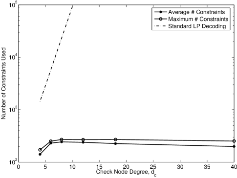
Figure 1: The average and maximum number of parity-check constraints used versus check node degree, $d_{c}$, for fixed length $n=360$ and rate $R=\frac{1}{2}$.

​​​​​​​​

In the second case, we studied random (3,6) codes of lengths $n=30$ to $n=1920$. For all values of $n$, the average (resp. maximum) number of required iterations remained between $5$ and $11$ (resp. $10$ and $16$). The average and maximum numbers of parity-check constraints in the final iteration are plotted versus $n$ in Fig. 2. We observe that the number of constraints is generally between $0.6n$ and $0.7n$.

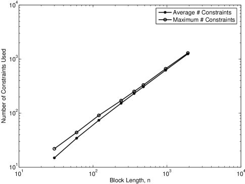
Figure 2: The average and maximum number of parity-check constraints used versus block length, $n$, for fixed rate $R=\frac{1}{2}$ and check node degree $d_{c}=6$.

​​​​​​​​

In the third experiment, we investigated the effect of the rate of the code on the performance of the algorithm. Fig. 3 shows the average and maximum numbers of parity-check constraints in the final iteration where the block length is $n=120$ and the number of parity checks, $m$, increases from $15$ to $90$. The variable node degree is fixed at $d_{v}=3$. We see that the average and maximum numbers of constraints are respectively in the ranges $1.1m$ to $1.2m$ and $1.4m$ to $1.6m$ for most values of $m$. The relatively large drop in the average number for $m=90$ with respect to the linear curve can be explained by the fact that at this value of $m$ the rate of failure of LP decoding was less than $0.5$ at $-1.0$ dB, whereas for all the other values of $m$, this rate was close to $1$. Since the success of LP decoding generally indicates proximity of the received vector to a codeword, we expect the number of parity checks required to converge to be small in such a case, which decreases the average number of constraints.

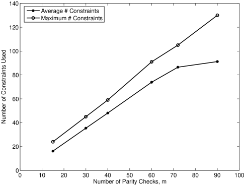
Figure 3: The average and maximum number of parity-check constraints used versus the number of parity checks, $m$, for $n=120$ and $d_{v}=3$.

​​​​​​​​

Finally, in Fig. 4, we compare the average decoding time of different algorithms at the low SNR of $-1.0$ dB. It is important to note that the running times of the LP-based techniques strongly depend on the underlying LP solver. In this work, we have used the open-source GNU Linear Programming Kit (GLPK [4]) for solving the LPs. The numerical results demonstrate that the adaptive algorithm significantly reduces the gap between the speed of standard LP decoding and that of the sum-product message-passing algorithm. Comparing the results for the (3,6) codes (dashed lines) and the (4,8) codes (solid lines) further shows that while the decoding time for the standard LP increases very rapidly with the check node degree of the code, the adaptive technique is not significantly affected by the change in the check node degree.

Our simulations indicate that the decoding time of the adaptive algorithm does not change significantly even if the code has a high-density parity-check matrix. This result can be explained by two factors. First, Fig. 1 shows that the number of constraints used in the algorithm does not change with the check node degree of the code. Second, while having a smaller check degree makes the matrix of constraints sparser, the LP solver that we are using does not benefit from this sparsity. A similar behavior was also observed when we used a commercial LP solver, MOSEK, instead of GLPK. We expect that by designing a special LP solver than can effectively take advantage of the sparsity of this problem, the time complexities of the LP-based techniques may become closer to those of the message-passing techniques.

Fig. 4 also shows the average decoding time when warm starts are used in the iterations of the adaptive decoding algorithm. We can see that warm starts slightly decrease the slope of the decoding-time curve when plotted against the logarithm of the block length. This translates into approximately a factor of 3 improvement in the decoding time at a block length of 1000.

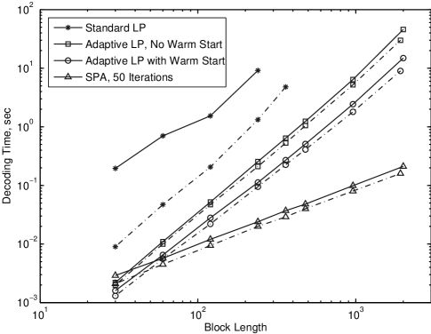
Figure 4: The average decoding time versus the length of the code for regular (3,6) LDPC codes (dashed lines) and (4,8) LDPC codes (solid lines) at SNR=$-1.0$ dB.

​​​​​​​​

Based on the simulation results, we observe that in practice the algorithm performs much faster than is guaranteed by Theorem 2. These observations suggest the following conjecture.

Conjecture 1

For a random parity-check code of length $n$ with $m=n(1-R)$ parity checks and arbitrary degree distributions, as $n$ and $m$ increase, the adaptive LP decoding algorithm converges with probability arbitrarily close to $1$ in at most $\alpha$ iterations and with at most an average of $\beta$ final parity-check constraints per check node, where $\alpha$ and $\beta$ are constants independent of the length, rate and degree distribution of the code.

IV Generating Cuts to Improve the Performance

The complexity reduction obtained by adaptive LP decoding inspires the use of cutting-plane techniques to improve the error rate performance of the algorithm. Specifically, when LP with all the original constraints gives a nonintegral solution, we try to cut the current solution, while keeping all the possible integral solutions (codewords) feasible.

In the decoding problem, the new cuts can be chosen from a pool of constraints describing a relaxation of the maximum-likelihood problem which is tighter than the fundamental polytope. In this sense, the cutting-plane technique is equivalent to the adaptive LP decoding of the previous section, with the difference that there are more constraints to choose from. The effectiveness of this method depends on how closely the new relaxation approximates the ML decoding problem, and how efficiently we can search for those constraints that introduce cuts. Feldman et al. [1] have mentioned some ways to tighten the relaxation of the ML decoding, including adding redundant parity checks (RPC), and using lift-and-project methods. (For more on lift-and-project, see [5] and references therein.) Gomory’s algorithm [6] is also one of the most well-known techniques for general integer optimization problems, although it suffers from slow convergence. Each of these methods can be applied adaptively in the context of cutting-plane techniques.

The simple structure of RPCs makes them an interesting choice for generating cuts. There are examples, such as the dual code of the (4,7) Hamming code, where even the relaxation obtained by adding all the possible RPC constraints does not guarantee convergence to a codeword. In other words, it is possible to obtain a nonintegral solution for which there is no RPC cut. Understanding the effect of RPCs in general requires further study. Also, finding efficient methods to search for RPC cuts for a given nonintegral solution remains an open issue. On the other hand, as observed in simulation results, RPC cuts are generally strong, and a reasonable number of them makes the resulting LP relaxation tight enough to converge to an integer-valued solution. In this work, we focus on cutting-plane algorithms that use RPC cuts.

IV-A Finding Redundant Parity-Check Cuts

An RPC is obtained by modulo-2 addition of some of the rows of the parity-check matrix, and this new check introduces a number of constraints that may include a cut. There is an exponential number of RPCs that can be made this way, and in general, most of them do not introduce cuts. Hence, we need to find the cuts efficiently by exploiting the particular structure of the decoding problem. In particular, we observe that cycles in the graph have an important role in determining whether an RPC generates a cut. To explain this property, we start with some definitions.

Definition 2

Given a current solution, $\underline{x}$, the subset $T\subset\{1,2,\ldots,m\}$ of check nodes is called a cut-generating collection if the RPC made by modulo-2 addition of the parity-checks corresponding to $T$ introduces a cut. If no proper of $T$ other that itself has this property, we call it a minimal cut-generating collection.

Definition 3

Given a pseudo-codeword $\underline{x}$, we denote by $\phi$ the set of variable nodes in the Tanner graph of the code whose corresponding elements in $\underline{x}$ have fractional values. Also, let $F$ be the subgraph made up of these variable nodes, the check nodes directly connected to them, and all the edges that connect them. We call $F$ the fractional subgraph and any cycle in $F$ a fractional cycle at $\underline{x}$.

Theorem 3 below explains the relevance of the concept of fractional cycles. Its proof makes use of the following lemma.

Lemma 2

Suppose that $c_{1}$ and $c_{2}$ are two parity checks whose constraints are satisfied by the current solution, $\underline{x}$. Then, $c\triangleq c_{1}\oplus c_{2}$, the modulo-2 combination of these checks, can generate a cut only if the neighborhoods of $c_{1}$ and $c_{2}$ have at least two fractional-valued variable nodes in common.

Proof:

See Appendix I. ∎

Theorem 3

Let $T$ be a collection of check nodes in the Tanner graph of the code. If $T$ is a cut-generating collection at $\underline{x}$, then there exists a fractional cycle such that all the check nodes on it belong to $T$.

Proof:

We first consider the case where $T$ is a minimal cut-generating collection. Note that any cut-generating collection must contain at least two check nodes, since no single check node generates a cut. Pick an arbitrary check node $c_{j}$ in $T$. We make an RPC $c_{r}$ by linearly combining the parity checks in $T\backslash\{c_{j}\}$. From Lemma 2 and the minimality of $T$, it follows that there are at least two fractional-valued variable nodes common to the neighborhoods of $c_{j}$ and $c_{r}$. Applying this reasoning to every check node in $T$, we conclude that any check node in the collection $T$ is connected to at least two fractional-valued variable nodes of degree at least 2. Therefore, the subgraph $G$ corresponding to the check nodes in $T$ and their neighboring variable nodes must contain a cycle which passes through only fractional-valued variable nodes, as claimed.

If $T$ is not a minimal cut-generating collection, then it must contain a minimal cut-generating collection, $T_{0}$. To see this, observe that there must be a check node in $T$ whose removal leaves a cut-generating collection of check nodes. Iteration of this check node removal process must terminate in a non-empty minimal cut-generating collection $T_{0}$ containing at least two check nodes. The subgraph $G_{0}$ corresponding to $T_{0}$ is contained in the subgraph $G$ corresponding to $T$, so the fractional cycle in $G_{0}$ constructed as above is also a fractional cycle in $G$.

∎

The following theorem confirms that a fractional cycle always exists for any non-integer pseudocodeword. We can represent the fractional subgraph $F$ corresponding to the pseudocodeword $\underline{x}$ as a union of disjoint, connected subgraphs $\{F_{i}\}$, $i=1,\cdots,K$, for some $K\geq 1$. We refer to each connected subgraph $F_{i}$ as a cluster.

Theorem 4

Let $\underline{x}$ be the solution of an LP decoding problem with Tanner graph $G$ and log-likelihood vector $\gamma$. Let $F$ denote the fractional subgraph corresponding to $\underline{x}$. Then each cluster $F_{i}$, $i=1,\cdots,K$ in $F$ contains a cycle.

Proof:

See Appendix II. ∎

The results above motivate the following algorithm to search for RPC cuts.

Algorithm 3

Step 1: Given a solution $\underline{x}$, prune the Tanner graph by removing all the variable nodes with integer values.

Step 2: Starting from an arbitrary check node, randomly walk through the pruned graph until a cycle is found.

Step 3: Create an RPC by combining the rows of the parity-check matrix corresponding to the check nodes in the cycle.

Step 4: If this RPC introduces a cut, add it to the Tanner graph and exit; otherwise go to Step 2.

When the fractional subgraph contains many cycles and it is feasible to check only a small fraction of them, the randomized method described above can efficiently find cycles. However, when the cycles are few in number, this algorithm may actually check a number of cycles several times, while skipping some others. In this case, a structured search, such as one based on the depth-first search (DFS) technique, can be used to find all the simple cycles in the fractional subgraph. One can then check to see if any of them introduces an RPC cut. However, to guarantee that all the potential RPCs are checked, one will still need to modify this search to include complex cycles, as, in general, a complex cycle is more likely to generate an RPC cut than a simple cycle with a comparable number of edges.

As shown above, by exploiting some of the properties of the linear code LP decoding problem, one can expedite the search for RPC cuts. However, there remains a need for more efficient methods of finding RPC cuts.

IV-B Complexity Considerations

There are a number of parameters that determine the complexity of the adaptive algorithm with RPC cuts, including the number of iterations of Algorithm 3 to find a cut, the total number of cuts that are needed to obtain an integer solution, and the time taken by each run of the LP solver after adding a cut. In particular, we observe empirically that a number of cuts less than the length of the code is often enough to ensure convergence to the ML codeword. By using each solution of the LP as a warm start for the next iteration after adding further cuts, the time that each LP takes can be significantly reduced. For example, for a regular (3,4) code of length 100 with RPC cuts, although as many as 70 LP problems may have to be solved for a successful decoding, the total time that is spent on these LP problems is no more than 10 times that of solving the standard problem (with no RPC cuts). Moreover, if we allow more than one cut to be added per iteration, the number of these iterations can be further reduced.

Since Algorithm 3 involves a random search, there is no guarantee that it will find a cut (if one exists) in a finite number of iterations. In particular, we have observed cases where, even after a large number of iterations, no cut was found, while a number of RPCs were repeatedly visited. This could mean that either no RPC cut exists for these cases, or the cuts have a structure that makes them unlikely to be selected by our random search algorithm.

In order to control the complexity, we can impose a limit, $C^{max}$, on the number of iterations of the search, and if no cut is found after $C^{max}$ trials, we declare failure. By changing $C^{max}$, we can trade complexity with performance. Alternatively, we can put a limit, $T^{max}$, on the total time that is spent on the decoding process. In order to find a proper value for this maximum, we ran the algorithm with a very large value of $C^{max}$ and measured the total decoding time for the cases where the algorithm was successful in finding the ML solution. Based on these observations, we found that 10 times the worst-case running time of the adaptive LP decoding algorithm of Section III serves as a suitable value for $T^{max}$.

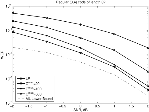
Figure 5: WER of cutting-plane LP versus SNR for different values of $C^{max}$.

​​​​​​​​

IV-C Numerical Results

To demonstrate the performance improvement achieved by using the RPC cutting-plane technique, we present simulation results for random regular $(3,4)$ LDPC codes on the AWGN channel. We consider codes of length 32, 100, and 240 bits.

In Fig. 5, for the length-32 code, we plot the word error rate (WER) versus SNR for different values of $C^{max}$, demonstrating the trade-off between performance and complexity. As in all subsequent figures, the SNR is defined as the ratio of the variance of the transmitted discrete-time signal to the variance of the noise sample.

For purposes of comparison, the WER of LP decoding with no RPC cut, as well as a lower bound on the WER of the ML decoder have been included in the figure. In order to obtain the ML lower bound, we counted the number of times that the cutting-plane LP algorithm, using a large value of $C^{max}$, converged to a codeword other than the transmitted codeword, and then divided that by the number of blocks. Due to the ML certificate property of LP decoding, we know that ML decoding would fail in those cases, as well. On the other hand, ML decoding may also fail in some of the cases where LP decoding does not converge to an integral solution. Therefore, this estimate gives a lower bound on the WER of ML decoding.

However, this method for computing the ML lower bound could not be applied to the codes of length greater that 32 bits. Therefore, as an alternative, we used the performance of the Box-and-Match soft decision decoding algorithm (BMA) developed by Valembois and Fossorier [8] as an approximation of the ML decoder performance.

In Figs. 6-8, the performance of LP decoding with RPC cuts is compared to that of standard LP decoding, sum-product decoding, and also the BMA. Each figure corresponds to a fixed block length, and in all three cases the sum-product decoding had 100 iterations. The curves show that, as the SNR increases, the proposed method outperforms the LP and the SPA, and significantly closes the gap to the ML decoder performance. However, one can see that, as the code length increases, the relative improvement provided by RPC cuts becomes less pronounced. This may be due to the fact that, for larger code lengths, the Tanner graph becomes more tree-like, and therefore the negative effect of cycles on LP and message-passing decoding techniques becomes less important, especially at low SNR.

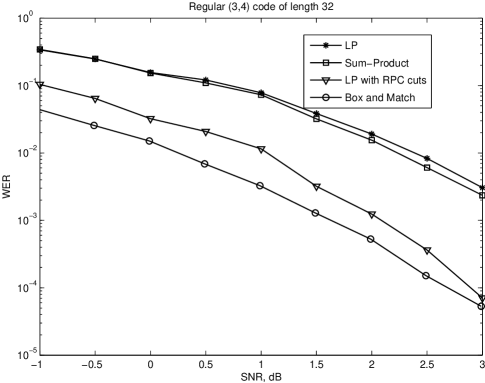
Figure 6: WER of cutting-plane LP versus SNR for length 32 and maximum decoding time 10 times that of the LP decoding.

​​​​​​​​

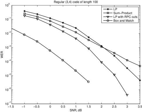
Figure 7: WER of cutting-plane LP versus SNR for length 100 and maximum decoding time 10 times that of the LP decoding.

​​​​​​​​

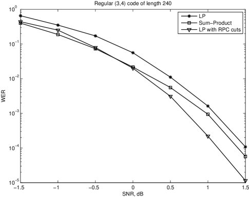
Figure 8: WER of cutting-plane LP versus SNR for length 240 and maximum decoding time 10 times that of the LP decoding.

​​​​​​​​

V Conclusion

In this paper, we studied the potential for improving LP decoding, both in complexity and performance, by using an adaptive approach. Key to this approach is the ML certificate property of LP decoders, that is, the ability to detect the failure to find the ML codeword. This property is shared by message-passing decoding algorithms only in specific circumstances, such as on the erasure channel. The ML certificate property makes it possible to selectively and adaptively add only those constraints that are “useful,” depending on the current status of the LP decoding process.

We proposed an adaptive LP decoding algorithm with decoding complexity that is independent of the code degree distributions, making it possible to apply LP decoding to parity-check codes of arbitrary densities. However, since general purpose LP solvers are used at each iteration, the complexity is still a super-linear function of the block length, as opposed to a linear function as achieved by the message-passing decoder. It remains an open question whether special LP solvers for decoding of LDPC codes might take advantage of the sparsity of the constraints and other properties of the LP decoding problem to provide linear complexity.

We also explored the application of cutting-plane techniques in LP decoding. We showed that redundant parity checks provide strong cuts, even though they may not guarantee ML performance. The results indicate that it would be worthwhile to find more efficient ways to search for strong RPC cuts by exploiting their properties, as well as to determine specific classes of codes for which RPC cuts are particularly effective. It would also be interesting to investigate the effectiveness of cuts generated by other techniques, such as lift-and-project cuts, Gomory cuts, or cuts specially designed for this decoding application.

Appendix A proof of Lemma 2

Proof:

Let $N_{1}$, $N_{2}$, and $N$ denote the sets of variable nodes in the neighborhoods of $c_{1}$, $c_{2}$, and $c$, respectively, and define $S\triangleq N_{1}\cap N_{2}$. Hence, we will have $N=(N_{1}\cup N_{2})\backslash S$. We can write $S$ as a union of disjoint sets $S_{0}$, $S_{1}$, and $S_{f}$, where they respectively represent the members of $S$ whose values are equal to $0$, equal to $1$, or in the range $(0,1)$. In order to prove the lemma, it is enough to show that $|S_{f}|\geq 2$.

Parity check $c$ generates a cut, hence there is an odd-sized subset $V\subset N$ of its neighborhood, for which we can write

$$\sum_{i\in V}x_{i}-\sum_{i\in N\backslash V}x_{i}>|V|-1.$$ (16)

Since $N_{1}$ and $N_{2}$ have no common member in $N$, we can write

$$V=V_{1}\cup V_{2},$$ (17)

where $V_{1}\subset N_{1}\backslash S$ and $V_{2}\subset N_{2}\backslash S$ are disjoint, and exactly one of them has an odd size. and $|V_{2}|$ is even. Now, (16) can be rewritten as

$$M\triangleq\sum_{i\in V_{1}}x_{i}+\sum_{i\in V_{2}}x_{i}-\sum_{i\in N_{1}\backslash V_{1}\backslash S}x_{i}-\sum_{i\in N_{2}\backslash V_{2}\backslash S}x_{i}>|V_{1}|+|V_{2}|-1.$$ (18)

Since $c_{1}$ and $c_{2}$ do not generate cuts, all the constraints they introduce should be satisfied by $\underline{x}$. Now consider the two sets $V_{1}\cup S_{1}$ and $V_{2}\cup S_{1}$. As $S_{1}$ is disjoint from both $V_{1}$ and $V_{2}$, and exactly one of $V_{1}$ and $V_{2}$ is odd-sized, we further conclude that exactly one of $V_{1}\cup S_{1}$ and $V_{2}\cup S_{1}$ is odd-sized, as well. Without loss of generality, assume that $|V_{1}\cup S_{1}|$ is odd and $|V_{2}\cup S_{1}|$ is even.

Depending on whether $|S_{f}|$ is even or odd, we proceed by dividing the problem into two cases:

Case 1 ( $|S_{f}|$ is even): Consider the following constraint given by $c_{1}$

$$\sum_{i\in V_{1}}x_{i}+\sum_{i\in S_{1}}x_{i}+\sum_{i\in S_{f}}x_{i}-\sum_{i\in N_{1}\backslash(V_{1}\cup S_{1}\cup S_{f})}x_{i}\leq|V_{1}|+|S_{1}|+|S_{f}|-1.$$ (19)

Since $\sum_{i\in S_{1}}x_{i}=|S_{1}|$ and $\sum_{i\in S_{0}}x_{i}=0$, we can simplify (19) as

$$\sum_{i\in V_{1}}x_{i}+\sum_{i\in S_{f}}x_{i}-\sum_{i\in N_{1}\backslash(V_{1}\cup S)}x_{i}\leq|V_{1}|+|S_{f}|-1.$$ (20)

Now, starting from (18) and using the fact that $N_{1}\backslash(V_{1}\cup S)\subset N\backslash V$, we have

$$|V_{1}|+|V_{2}|-1\!\!\! < \!\!\!M=\sum_{i\in V_{1}}x_{i}+\sum_{i\in V_{2}}x_{i}-\sum_{i\in N\backslash V}x_{i}$$ (21)

$$< \!\!\!\sum_{i\in V_{1}}x_{i}+\sum_{i\in V_{2}}x_{i}-\sum_{i\in N_{1}\backslash(V_{1}\cup S)}x_{i}$$

$$\leq \!\!\!|V_{1}|+\sum_{i\in V_{2}}x_{i}-1+|S_{f}|-\sum_{i\in S_{f}}x_{i},$$

where for the last inequality we used (20). Since $\sum_{i\in V_{2}}x_{i}\leq|V_{2}|$, (21) yields

$$|V_{1}|+|V_{2}|-1<|V_{1}|+|V_{2}|-1+|S_{f}|-\sum_{i\in S_{f}}x_{i},$$ (22)

Hence, $S_{f}$ is a non-empty set, and since it is even in size, we must have $|S_{f}|\geq 2$.

Case 2 ( $|S_{f}|$ is odd): In this case, we swap the roles of $c_{1}$ and $c_{2}$, and write for $c_{2}$

$$\sum_{i\in V_{2}}x_{i}+\sum_{i\in S_{1}}x_{i}+\sum_{i\in S_{f}}x_{i}-\sum_{i\in N_{2}\backslash(V_{2}\cup S_{1}\cup S_{f})}x_{i}\leq|V_{2}|+|S_{1}|+|S_{f}|-1,$$ (23)

and for $c_{1}$

$$\sum_{i\in V_{1}}x_{i}+\sum_{i\in S_{1}}x_{i}-\sum_{i\in N_{1}\backslash(V_{1}\cup S_{1}\cup S_{f})}x_{i}-\sum_{i\in S_{f}}x_{i}\leq|V_{1}|+|S_{1}|-1.$$ (24)

By adding (23) and (24), we obtain after some cancellation

$$\sum_{i\in V_{1}}x_{i}+\sum_{i\in V_{2}}x_{i}-\sum_{i\in N_{1}\backslash(V_{1}\cup S)}x_{i}-\sum_{i\in N_{2}\backslash(V_{2}\cup S)}x_{i}\leq|V_{1}|+|V_{2}|+|S_{f}|-2.$$ (25)

Note that

$$N\backslash V=[N_{1}\backslash(V_{1}\cup S)]\cup[N_{2}\backslash(V_{2}\cup S)].$$ (26)

Hence, combining (18) and (25) yields

$$|V_{1}|+|V_{2}|-1<|V_{1}|+|V_{2}|+|S_{f}|-2,$$ (27)

which means that $|S_{f}|\geq 2$. ∎

Appendix B Proof of Theorem 4

Proof:

Assume, to the contrary, that for some $i\in\{1,\ldots,K\}$ the cluster $F_{i}\subseteq F$ is a tree. Denote by $V=\{v_{1},\cdots,v_{r}\}$ the set of indices of variable nodes of the Tanner graph that are in $F_{i}$, and by $V^{C}$ the complement of this set with respect to $I=\{1,\cdots,n\}$. For a vector $\underline{u}$ of length $n$ and any set $A\subset I$, let $\underline{u}_{A}$ represent the projection of $\underline{u}$ onto the coordinate indices in $A$. Using this notation, we note that $x_{V}\in(0,1)^{r}$.

We now show that there exists a point $\underline{x^{\prime}}$ in the fundamental polytope for which $\underline{x^{\prime}}_{V}\in\{0,1\}^{r}$, $\underline{x^{\prime}}_{V^{C}}=\underline{x}_{V^{C}}$, and $\underline{\gamma}^{T}\underline{x^{\prime}}\leq\underline{\gamma}^{T}\underline{x}$. That is, we identify a point in the fundamental polytope with cost strictly lower than the cost of $\underline{x}$, contradicting the fact that $\underline{x}$ is a solution to the LP problem.

To accomplish this, we formulate an LP decoding subproblem on a Tanner graph $\hat{G}$, which is constructed as follows. Let $G^{\prime}$ be the union of $F_{i}$ with all the edges and variable nodes in $G\backslash F_{i}$ that were directly connected to a check node of $F_{i}$ in the original graph, $G$. Clearly, since $F_{i}$ is disjoint from the other connected components of $F$, any such variable node $v$ lies in $G\backslash F$ and therefore has an integer value $x_{v}$ in the solution $\underline{x}$.

A variable node in $G^{\prime}\backslash F_{i}$ might be connected to $k>1$ check nodes in $F_{i}$, in which case $G^{\prime}$ will contain cycles. To break these cycles, we replicate any such variable node, creating $k$ distinct nodes, each connected to a distinct one of the $k$ check nodes. We refer to the resulting graph as $\hat{G}$, and think of $F_{i}$ as a subgraph of $\hat{G}$. We call the variable nodes in $F_{i}$ and $\hat{G}\backslash F_{i}$ basic and auxiliary variable nodes, respectively.

To each basic variable node $v$ in $F_{i}$, we assign the corresponding cost $\gamma_{v}$ in the original LP problem. To each auxiliary variable node $\hat{v}$ derived from a parent node $v$ in $G\backslash F_{i}$, we assign a cost $\Gamma$ or $-\Gamma$, according to whether the corresponding value $x_{v}$ in the pseudocodeword $\underline{x}$ is 0 or 1. Here $\Gamma$ is a positive constant that can be chosen, as described below, to ensure that, in the solution $\underline{\hat{x}}$ to the new LP subproblem on $\hat{G}$, the value $\hat{x}_{\hat{v}}$ of the auxiliary node $\hat{v}$ is equal to $x_{v}$.

Since $\hat{G}$ is now an acyclic Tanner graph, the solution, $\underline{\hat{x}}$, of LP decoding on this graph will be integral [7]. On the other hand, if we assign to each variable node in $\hat{G}$ the value of the corresponding parent node in the original solution, $\underline{x}$, the resulting vector, $\underline{x^{*}}$, will be another feasible point of the LP decoding subproblem on $\hat{G}$, since each check node in $\hat{G}$ sees the same set of variable node values in its neighborhood as does the corresponding check node in $G$ in the original LP decoding problem. Furthermore, we claim that if the cost $\Gamma$ is chosen to be larger than $\sum\limits_{j\in V}|\gamma_{j}|$, the values of the auxiliary variable nodes will be the same in $\underline{x^{*}}$ as in the integral optimal solution, $\underline{\hat{x}}$. This follows from the fact that, with the specified assignment of costs $\pm\Gamma$ to the auxiliary variable nodes, modifying the value in $\underline{x^{*}}$ of any such node increases the objective function by $\Gamma>\sum\limits_{j\in V}|\gamma_{j}|$. No modification of the values corresponding to basic variable nodes can compensate for this increase, since any such modification can decrease the objective function by at most $\sum\limits_{j\in V}|\gamma_{j}|$. Therefore, auxiliary variable nodes have the same values in both vectors, implying that

$$\sum\limits_{j\in V}\gamma_{j}\hat{x}_{j}<\sum\limits_{j\in V}\gamma_{j}{x^{*}}_{j}=\sum\limits_{j\in V}\gamma_{j}x_{j}.$$ (28)

We now define the vector $\underline{x^{\prime}}$ as

$$x^{\prime}_{j}=\begin{cases}\hat{x}_{j}\ &\text{if }j\in V,\\ x_{j}\ &\text{if }j\in V^{C}.\end{cases}$$ (29)

We know that $\underline{x^{\prime}}_{V}$ is integral, and (28) implies that $\underline{x^{\prime}}$ has a lower cost than $\underline{x}$. It only remains to show that $\underline{x^{\prime}}$ satisfies all the LP constraints introduced by the parity-checks of the original Tanner graph $G$.

Consider a check node $c_{j}\in G$. If $c_{j}\in F_{i}$, its neighboring variable nodes will have the same set of values as in the solution $\underline{\hat{x}}$ of LP decoding on $\hat{G}$, and therefore all its corresponding LP constraints will be satisfied. If $c_{j}\notin F_{i}$, all of its neighboring variable nodes are in $V^{C}$, and they too have the same values as in $\underline{x}$. Hence the LP constraints that $c_{j}$ introduces will be satisfied. It follows that $\underline{x^{\prime}}$ is a point in the fundamental polytope with lower cost than $\underline{x}$, contradicting the fact that $\underline{x}$ is the solution of the original LP decoding problem on $G$. Therefore, each component $F_{i}$ must contain a cycle.

∎

References

- [1] J. Feldman, M. J. Wainwright, and D. Karger, “Using linear programming to decode binary linear codes,” IEEE Trans. Inform. Theory, vol. 51, no. 3, pp. 954-972, Mar. 2005.
- [2] P. O. Vontobel and R. Koetter, “On the relationship between linear programming decoding and min-sum algorithm decoding,” Proc. Int’l Symp. on Inform. Theory and Applications, pp. 991-996, Parma, Italy, Oct. 2004.
- [3] P. O. Vontobel and R. Koetter, “Graph-cover decoding and finite-length analysis of message-passing iterative decoding of LDPC codes,” Sumbitted to IEEE Trans. Inform. Theory.
- [4] “GNU Linear Programming Kit,” Available at http://www.gnu.org/software/glpk.
- [5] M. Laurent, “A comparison of the Sherali-Adams, Lovász-Schrijver and Lasserre relaxations for 0-1 programming,” Mathematics of Operations Research, vol. 28, no. 3, pp. 470-496, 2003.
- [6] R. Gomory, “An algorithm for integer solutions to linear programs,” Princeton IBM Mathematical Research Report, Nov. 1958.
- [7] M. J. Wainwright, T. S. Jaakkola, and A. S. Willsky, “MAP estimation via agreement on trees: message-passing and linear programming,” IEEE Trans. Inform. Theory, vol. 51, vo. 11, pp. 3697-3717, Nov. 2005.
- [8] A. Valembois and M. Fossorier, “Box and Match techniques applied to soft decision decoding,” IEEE Trans. Inform. Theory, vol. 50, pp. 796-810, May 2004.