Maximum Weighted Sum Rate of Multi-Antenna Broadcast Channels

Abstract

Recently, researchers showed that dirty paper coding (DPC) is the optimal transmission strategy for multiple-input multiple-output broadcast channels (MIMO-BC). In this paper, we study how to determine the maximum weighted sum of DPC rates through solving the maximum weighted sum rate problem of the dual MIMO multiple access channel (MIMO-MAC) with a sum power constraint. We first simplify the maximum weighted sum rate problem such that enumerating all possible decoding orders in the dual MIMO-MAC is unnecessary. We then design an efficient algorithm based on conjugate gradient projection (CGP) to solve the maximum weighted sum rate problem. Our proposed CGP method utilizes the powerful concept of Hessian conjugacy. We also develop a rigorous algorithm to solve the projection problem. We show that CGP enjoys provable convergence, nice scalability, and great efficiency for large MIMO-BC systems.

I Introduction

The capacity region of multiple-input multiple-output broadcast channels (MIMO-BC) has received great attention in recent years. MIMO-BC belong to the class of nondegraded broadcast channels, for which the capacity region is notoriously hard to analyze [1]. Very recently, researchers have made significant progress in this area. Most notably, Weigarten et. al. finally proved the long-open conjecture in [2] that the “dirty paper coding” (DPC) strategy is the capacity achieving transmission strategy for MIMO-BC. Moreover, by the remarkable channel duality between MIMO-BC and its dual MIMO multiple access channel (MIMO-MAC) [3, 4, 5], the nonconvex MIMO-BC capacity region (with respect to the input covariance matrices) can be transformed to the convex dual MIMO-MAC capacity region with a sum power constraint.

In this paper, we study how to determine the maximum weighted sum of DPC rates (MWSR) of MIMO-BC through solving the maximum weighted sum rate problem of the dual MIMO-MAC. Important applications of the MWSR problem of MIMO-BC include but are not limited to applying Lagrangian dual decomposition for the cross-layer optimization for MIMO-based mesh networks [6]. The MWSR problem of MIMO-BC is the general case of the maximum sum rate problem (MSR) of MIMO-BC, which has been solved by using various algorithms in the literature. Such algorithms include the minimax method (MM) by Lan and Yu [7], the steepest descent (SD) method by Viswanathan et al. [8], the dual decomposition (DD) method by Yu [9], two iterative water-filling methods (IWFs) by Jindal et al.[10], and the conjugate gradient projection method recently proposed by us [11]. Among these algorithms, IWFs and CGP appear to be the simplest. However, all of these existing algorithms have limitations in that they cannot be readily extended to the MWSR problem of MIMO-BC. As we show later, the objective function of the MWSR problem has a very different and much more complex objective function. The aforementioned algorithms can only handle the objective function of MSR, which is just a special case of MWSR (by setting all weights to one). These limitations of the existing algorithms motivate us to design an efficient and scalable algorithm with a modest storage requirement to solve the MWSR problem of large MIMO-BC systems.

In this paper, we significantly extend our CGP method in [11] to handle the MWSR problem of MIMO-BC. Our CGP method is inspired by [12], where a gradient projection method was used to heuristically solve the MSR problem of MIMO interference channels. However, unlike [12], we use the conjugate gradient directions instead of gradient directions to eliminate the “zigzagging” phenomenon. Also different from [12], we develop a rigorous algorithm to exactly solve the projection problem. Our main contributions in this paper are three-fold:

1. To the best of our knowledge, our paper is the first work that considers the MWSR problem of MIMO-BC. Studying the MWSR problem is more useful and more important because the MWSR problem is the general case of MSR, and it has much wider application in systems and networks that employ MIMO-BC.

2. We simplify the MWSR problem of the dual MIMO-MAC such that enumerating all different decoding orders in the dual MIMO-MAC is unnecessary, thus paving the way to design an algorithm to efficiently solve the MWSR problem of MIMO-BC.

3. We extend the CGP method in [11] for the MWSR problem of MIMO-BC. This extended CGP method still enjoys provable convergence as well as nice scalability, and has the desirable linear complexity. Also, the extended CGP method is insensitive to the increase of the number of users and has a modest memory requirement.

The remainder of this paper is organized as follows. In Section II, we discuss the network model and the problem formulation. Section III introduces the key components in of CGP, including the computation of conjugate gradients and performing projection. We analyze the complexity of CGP in Section IV. Numerical results of CGP’s convergence behavior and performance comparison with other existing algorithms are presented in Section V. Section VI concludes this paper.

II System Model and Problem Formulation

We begin with introducing notations. We use boldface to denote matrices and vectors. For a complex-valued matrix $\mathbf{A}$, $\mathbf{A}^{*}$ and $\mathbf{A}^{{\dagger}}$ denote the conjugate and the conjugate transpose of $\mathbf{A}$, respectively. $\mathrm{Tr}\{\mathbf{A}\}$ denotes the trace of $\mathbf{A}$. We let $\mathbf{I}$ denote the identity matrix with dimension determined from context. $\mathbf{A}\succeq 0$ represents that $\mathbf{A}$ is Hermitian and positive semidefinite (PSD). Diag$\left\{\mathbf{A}_{1}\ldots\mathbf{A}_{n}\right\}$ denotes the block diagonal matrix with matrices $\mathbf{A}_{1},\ldots,\mathbf{A}_{n}$ on its main diagonal.

Suppose that a MIMO Gaussian broadcast channel has $K$ users, each of which is equipped with $n_{r}$ antennas, and the transmitter has $n_{t}$ antennas. The channel matrix for user $i$ is denoted as $\mathbf{H}_{i}\in\mathbb{C}^{n_{r}\times n_{t}}$. In [2], it has been shown that the capacity region of MIMO-BC is equal to the dirty-paper coding region (DPC). In DPC rate region, suppose that users $1,\ldots,K$ are encoded subsequently, then the rate of user $i$ can be computed as [3]

$$R_{i}^{\mathrm{DPC}}(\mathbf{\Gamma})=\log\frac{\det\left(\mathbf{I}+\mathbf{H}_{i}\left(\sum_{j=i}^{K}\mathbf{\Gamma}_{j}\right)\mathbf{H}_{i}^{{\dagger}}\right)}{\det\left(\mathbf{I}+\mathbf{H}_{i}\left(\sum_{j=i+1}^{K}\mathbf{\Gamma}_{j}\right)\mathbf{H}_{i}^{{\dagger}}\right)},$$ (1)

where $\mathbf{\Gamma}_{i}\in\mathbb{C}^{n_{t}\times n_{t}}$, $i=1,\ldots,K$, are the downlink input covariance matrices, $\mathbf{\Gamma}\triangleq\{\mathbf{\Gamma}_{1},\ldots\mathbf{\Gamma}_{K}\}$ denotes the collection of all the downlink covariance matrices. As a result, the MWSR problem can then be written as follows:

$$\begin{array}[]{rl}\mbox{Maximize}&\sum_{i=1}^{K}u_{i}R_{i}^{\mathrm{DPC}}(\mathbf{\Gamma})\\ \mbox{subject to}&\mathbf{\Gamma}_{i}\succeq 0,\quad i=1,\ldots,K\\ &\sum_{i=1}^{K}\mathrm{Tr}(\mathbf{\Gamma}_{i})\leq P,\end{array}$$ (2)

where $u_{i}$ is the weight of user $i$, $P$ represents the maximum transmit power at the transmitter. It is evident that (2) is a nonconvex optimization problem since the DPC rate equation in (1) is neither a concave nor a convex function in the input covariance matrices $\mathbf{\Gamma}_{1},\ldots,\mathbf{\Gamma}_{K}$. However, the authors in [3] showed that due to the duality between MIMO-BC and MIMO-MAC, the rates achievable in MIMO-BC are also achievable in MIMO-MAC. That is, given a feasible $\mathbf{\Gamma}$, there exists a set of feasible uplink input covariance matrices for the dual MIMO-MAC, denoted by $\mathbf{Q}$, such that $R_{i}^{\mathrm{MAC}}(\mathbf{Q})=R_{i}^{\mathrm{DPC}}(\mathbf{\Gamma})$. Thus, (2) is equivalent to the following maximum weighted sum rate problem of the dual MIMO-MAC with a sum power constraint:

$$\begin{array}[]{rl}\mbox{Maximize}&\sum_{i=1}^{K}u_{i}R_{i}^{\mathrm{MAC}}(\mathbf{Q})\\ \mbox{subject to}&\mathbf{Q}_{i}\succeq 0,\quad i=1,\ldots,K\\ &R_{i}^{\mathrm{MAC}}(\mathbf{Q})\in\mathcal{C}_{\mathrm{MAC}}(P,\mathbf{H}^{{\dagger}}),\,\,i=1,\ldots,K\\ &\sum_{i=1}^{K}\mathrm{Tr}(\mathbf{Q}_{i})\leq P,\\ \end{array}$$ (3)

where $\mathbf{Q}_{i}\in\mathbb{C}^{n_{r}\times n_{r}}$, $i=1,\ldots,K$, are the uplink input covariance matrices, $\mathbf{Q}\triangleq\{\mathbf{Q}_{1},\ldots\mathbf{Q}_{K}\}$ represents the collection of all the uplink covariance matrices, $\mathcal{C}_{\mathrm{MAC}}(P,\mathbf{H}^{{\dagger}})$ represents the capacity region of the dual MIMO-MAC. It is known that the capacity region of a MIMO-MAC can be achieved by the successive decoding [1]. However, in order to determine the capacity region of a MIMO-MAC, all possible successive decoding orders need to be enumerated, which is very cumbersome. In the following theorem, however, we show that the enumeration of all successive decoding orders is indeed unnecessary when solving the MWSR problem of the dual MIMO-MAC. This result significantly reduces the complexity and paves the way to efficiently solve the MWSR problem by using CGP method.

Theorem 1

The MWSR problem in (3) can be solved by the following equivalent optimization problem:

$$\begin{array}[]{rl}\!\!\!\!\!\!\mbox{Maximize}&\!\!\!\sum_{i=1}^{K}(u_{\pi(i)}-u_{\pi(i-1)})\times\\ \!\!\!\!\!\!&\!\!\!\log\det\left(\mathbf{I}+\sum_{j=i}^{K}\mathbf{H}_{\pi(j)}^{{\dagger}}\mathbf{Q}_{\pi(j)}\mathbf{H}_{\pi(j)}\right)\\ \!\!\!\!\!\!\mbox{subject to}&\!\!\!\sum_{i=1}^{K}\mathrm{Tr}(\mathbf{Q}_{i})\leq P_{\max}\\ \!\!\!\!\!\!&\!\!\!\mathbf{Q}_{i}\succeq 0,\,\,i=1,\ldots,K,\end{array}$$ (4)

where $u_{\pi(0)}\triangleq 0$, $\pi$ is a permutation of the set $\{1,\ldots,K\}$ such that $u_{\pi(1)}\leq\ldots\leq u_{\pi(K)}$. $\pi(i),i=1,\ldots,K$, represents the $i^{th}$ position in permutation $\pi$.

Proof:

Let $\Phi(\mathcal{S})=\log\det(\mathbf{I}+\sum_{i\in\mathcal{S}}\mathbf{H}_{\pi(i)}^{{\dagger}}\mathbf{Q}_{\pi(i)}\mathbf{H}_{\pi(i)})$, where $\mathcal{S}$ is a non-empty subset of $\{1,\ldots,K\}$. From Theorem 14.3.5 in [1], we know that the maximum weighted sum rate problem can be written as

$$\begin{array}[]{rl}\mbox{Maximize}&\sum_{i=1}^{K}u_{\pi(i)}R_{\pi(i)}^{\mathrm{MAC}}\\ \mbox{subject to}&\sum_{i\in\mathcal{S}}R_{\pi(i)}^{\mathrm{MAC}}\leq\Phi(\mathcal{S}),\,\,\forall\mathcal{S}\subseteq\{1,\ldots,K\}.\end{array}$$

Thus, it is not difficult to see that, when $\mathcal{S}=\{\pi(i)\}$, $R_{\pi(i)}^{\mathrm{MAC}}\leq\Phi(\{\pi(i)\})=\log\det\left(\mathbf{I}+\mathbf{H}_{\pi(i)}^{{\dagger}}\mathbf{Q}_{\pi(i)}\mathbf{H}_{\pi(i)}\right)$. Since $u_{\pi(1)}\leq\ldots\leq u_{\pi(K)}$, from Karush-Kuhn-Tucker (KKT) condition, we must have that the constraint $R_{\pi(K)}^{\mathrm{MAC}}\leq\Phi(\{\pi(K)\})$ must be tight at optimality. That is,

$$R_{\pi(K)}^{\mathrm{MAC}}=\log\det\left(\mathbf{I}+\mathbf{H}_{\pi(K)}^{{\dagger}}\mathbf{Q}_{\pi(K)}\mathbf{H}_{\pi(K)}\right).$$ (5)

Likewise, when $\mathcal{S}=\{\pi(K-1),\pi(K)\}$, we have

$$\begin{array}[]{l}R_{\pi(K-1)}^{\mathrm{MAC}}+R_{\pi(K)}^{\mathrm{MAC}}\leq\log\det\left(\mathbf{I}+\mathbf{H}_{\pi(K)}^{{\dagger}}\mathbf{Q}_{\pi(K)}\mathbf{H}_{\pi(K)}\right.\\ \hskip 72.26999pt\left.+\mathbf{H}_{\pi(K-1)}^{{\dagger}}\mathbf{Q}_{\pi(K-1)}\mathbf{H}_{\pi(K-1)}\right).\end{array}$$

So, from (5), we have

$$\begin{array}[]{l}R_{\pi(K-1)}^{\mathrm{MAC}}\leq\log\det\left(\mathbf{I}+\mathbf{H}_{\pi(K)}^{{\dagger}}\mathbf{Q}_{\pi(K)}\mathbf{H}_{\pi(K)}\right.\\ \hskip 57.81621pt\left.+\mathbf{H}_{\pi(K-1)}^{{\dagger}}\mathbf{Q}_{\pi(K-1)}\mathbf{H}_{\pi(K-1)}\right)-\\ \hskip 57.81621pt\log\det\left(\mathbf{I}+\mathbf{H}_{\pi(K)}^{{\dagger}}\mathbf{Q}_{\pi(K)}\mathbf{H}_{\pi(K)}\right).\end{array}$$ (6)

Since $u_{\pi(K-1)}$ is the second largest weight, again from KKT condition, we must have that (6) must be tight at optimality. This process continues for all $K$ users. Subsequently, we have that

$$\begin{array}[]{l}R_{\pi(i)}^{\mathrm{MAC}}=\log\det\left(\mathbf{I}+\sum_{j=i}^{K}\mathbf{H}_{\pi(j)}^{{\dagger}}\mathbf{Q}_{\pi(j)}\mathbf{H}_{\pi(j)}\right)\\ \hskip 28.90755pt-\log\det\left(\mathbf{I}+\sum_{j=i+1}^{K}\mathbf{H}_{\pi(j)}^{{\dagger}}\mathbf{Q}_{\pi(j)}\mathbf{H}_{\pi(j)}\right),\end{array}$$ (7)

for $i=1,\ldots,K-1$. Summing up all $u_{\pi(i)}R_{\pi(i)}^{\mathrm{MAC}}$ and after rearranging the terms, it is readily verifiable that

$$\begin{array}[]{l}\sum_{i=1}^{K}u_{\pi(i)}R_{\pi(i)}^{\mathrm{MAC}}=\sum_{i=1}^{K}(u_{\pi(i)}-u_{\pi(i-1)})\times\\ \hskip 72.26999pt\log\det\left(\mathbf{I}+\sum_{j=i}^{K}\mathbf{H}_{\pi(j)}^{{\dagger}}\mathbf{Q}_{\pi(j)}\mathbf{H}_{\pi(j)}\right).\end{array}$$

It then follows that the MWSR problem of the dual MIMO-MAC is equivalent to maximizing (II) with the sum power constraint, i.e., the optimization problem in (4). ∎

An important observation from (4) is that, since $\log\det\left(\cdot\right)$ is a concave function for positive semidefinite matrices [1], (4) is a convex optimization problem with respect to the uplink input covariance matrices $\mathbf{Q}_{\pi(1)},\ldots,\mathbf{Q}_{\pi(K)}$. However, although the standard interior point convex optimization method can be used to solve (4), it is considerably more complex than a method that exploits the special structure of (4).

III Conjugate Gradient Projection Method

In this paper, we modified the conjugate gradient projection method (CGP) in [11] to solve (4). CGP utilizes the important and powerful concept of Hessian conjugacy to deflect the gradient direction appropriately so as to achieve the superlinear convergence rate [13]. The framework of CGP for solving (4) is shown in Algorithm 1.

Algorithm 1 Gradient Projection Method

  Initialization:

   Choose the initial conditions $\mathbf{Q}^{(0)}=[\mathbf{Q}_{1}^{(0)},\mathbf{Q}_{2}^{(0)},\ldots,\mathbf{Q}_{K}^{(0)}]^{T}$. Let

   $k=0$.

  Main Loop:

   1. Calculate the conjugate gradients $\mathbf{G}_{i}^{(k)}$, $i=1,2,\ldots,K$.

   2. Choose an appropriate step size $s_{k}$. Let $\mathbf{Q}_{i}^{{}^{\prime}(k)}=\mathbf{Q}_{i}^{(k)}+s_{k}\mathbf{G}_{i}^{(k)}$,

    for $i=1,2,\ldots,K$.

   3. Let $\bar{\mathbf{Q}}^{(k)}$ be the projection of $\mathbf{Q}^{{}^{\prime}(k)}$ onto $\Omega_{+}(P)$, where $\Omega_{+}(P)\triangleq$

    $\{\mathbf{Q}_{i},\,\,i=1,\ldots,K|\mathbf{Q}_{i}\succeq 0,\sum_{i=1}^{K}\mathrm{Tr}\{\mathbf{Q}_{i}\}\leq P\}$.

   4. Choose appropriate step size $\alpha_{k}$. Let $\mathbf{Q}_{l}^{(k+1)}=\mathbf{Q}_{l}^{(k)}+\alpha_{k}(\bar{\mathbf{Q}}_{i}^{(k)}-$

    $\mathbf{Q}_{i}^{(k)})$, $i=1,2,\ldots,K$.

   5. $k=k+1$. If the maximum absolute value of the elements in $\mathbf{Q}_{i}^{(k)}-$

    $\mathbf{Q}_{i}^{(k-1)}<\epsilon$, for $i=1,2,\ldots,L$, then stop; else go to step 1.

Due to the complexity of the objective function in (4), we adopt the inexact line search method called “Armijo’s Rule” to avoid excessive objective function evaluations, while still enjoying provable convergence [13]. The basic idea of Armijo’s Rule is that at each step of the line search, we sacrifice accuracy for efficiency as long as we have sufficient improvement. According to Armijo’s Rule, in the $k^{th}$ iteration, we choose $\sigma_{k}=1$ and $\alpha_{k}=\beta^{m_{k}}$ (the same as in [12]), where $m_{k}$ is the first non-negative integer $m$ that satisfies

$$F(\mathbf{Q}^{(k+1)})-F(\mathbf{Q}^{(k)})\geq\sigma\beta^{m}\langle\mathbf{G}^{(k)},\bar{\mathbf{Q}}^{(k)}-\mathbf{Q}^{(k)}\rangle$$

$$=\sigma\beta^{m}\sum_{i=1}^{K}\mathrm{Tr}\left[\mathbf{G}_{i}^{{\dagger}(k)}\left(\bar{\mathbf{Q}}_{i}^{(k)}-\mathbf{Q}_{i}^{(k)}\right)\right],$$ (8)

where $0<\beta<1$ and $0<\sigma<1$ are fixed scalars.

Next, we will consider two major components in the CGP framework: 1) how to compute the conjugate gradient direction $\mathbf{G}_{i}$, and 2) how to project $\mathbf{Q}^{{}^{\prime}(k)}$ onto the set $\Omega_{+}(P)\triangleq\{\mathbf{Q}_{i},\,\,i=1,\ldots,K|\mathbf{Q}_{i}\succeq 0,\sum_{i=1}^{K}\mathrm{Tr}\{\mathbf{Q}_{i}\}\leq P\}$.

III-A Computing the Conjugate Gradients

The gradient $\bar{\mathbf{G}}_{\pi(j)}\triangleq\nabla_{\mathbf{Q}_{\pi(j)}}F(\mathbf{Q})$ depends on the partial derivative of $F(\mathbf{Q})$ with respect to $\mathbf{Q}_{\pi(j)}$. By using the formula $\frac{\partial\ln\det\left(\mathbf{A}+\mathbf{B}\mathbf{X}\mathbf{C}\right)}{\partial\mathbf{X}}=\left[\mathbf{C}(\mathbf{A}+\mathbf{B}\mathbf{X}\mathbf{C})^{-1}\mathbf{B}\right]^{T}$ [12, 14], we can compute the partial derivative of the $i^{th}$ term in the summation of $F(\mathbf{Q})$ with respect to $\mathbf{Q}_{\pi(j)}$, $j\geq i$, as follows:

$$\frac{\partial}{\partial\mathbf{Q}_{\pi(j)}}\Bigg{(}(u_{\pi(i)}-u_{\pi(i-1)})\times$$

$$\hskip 21.68121pt\left.\log\det\left(\mathbf{I}+\sum_{k=i}^{K}\mathbf{H}_{\pi(k)}^{{\dagger}}\mathbf{Q}_{\pi(k)}\mathbf{H}_{\pi(k)}\right)\right)$$

$$=\left(u_{\pi(i)}-u_{\pi(i-1)}\right)\times$$

$$\left[\mathbf{H}_{\pi(j)}\left(\mathbf{I}+\sum_{k=i}^{K}\mathbf{H}_{\pi(k)}^{{\dagger}}\mathbf{Q}_{\pi(k)}\mathbf{H}_{\pi(k)}\right)^{-1}\mathbf{H}_{\pi(j)}^{{\dagger}}\right]^{T}.$$

To compute the gradient of $F(\mathbf{Q})$ with respect to $\mathbf{Q}_{\pi(j)}$, we notice that only the first $j$ terms in $F(\mathbf{Q})$ involve $\mathbf{Q}_{\pi(j)}$. From the definition $\nabla_{z}f(z)=2(\partial f(z)/\partial z)^{*}$ [15], we have

$$\bar{\mathbf{G}}_{\pi(j)}=2\mathbf{H}_{\pi(j)}\Bigg{[}\sum_{i=1}^{j}\left(u_{\pi(i)}-u_{\pi(i-1)}\right)\times$$

$$\left.\left(\mathbf{I}+\sum_{k=i}^{K}\mathbf{H}_{\pi(k)}^{{\dagger}}\mathbf{Q}_{\pi(k)}\mathbf{H}_{\pi(k)}\right)^{-1}\right]\mathbf{H}_{\pi(j)}^{{\dagger}}.$$ (9)

It is worth to point out that we can exploit the special structure in (III-A) to significantly reduce the computation complexity in the implementation of the algorithm. Note that the most difficult part in computing $\bar{\mathbf{G}}_{\pi(j)}$ is the summation of the terms in the form of $\mathbf{H}_{\pi(k)}^{{\dagger}}\mathbf{Q}_{\pi(k)}\mathbf{H}_{\pi(k)}$. Without careful consideration, one may end up computing such additions $j(2K+1-j)/2$ times for $\bar{\mathbf{G}}_{\pi(j)}$. However, noting that most of the terms in the summation are still the same when $j$ varies, we can maintain a running sum for $\mathbf{I}+\sum_{k=i}^{K}\mathbf{H}_{\pi(k)}^{{\dagger}}\mathbf{Q}_{\pi(k)}\mathbf{H}_{\pi(k)}$, start out from $j=K$, and reduce $j$ by one sequentially. As a result, only one new term is added to the running sum in each iteration, which means we only need to do the addition once in each iteration.

The conjugate gradient direction in the $m^{th}$ iteration can be computed as $\mathbf{G}_{\pi(j)}^{(m)}=\bar{\mathbf{G}}_{\pi(j)}^{(m)}+\rho_{m}\mathbf{G}_{\pi(j)}^{(m-1)}$. We adopt the Fletcher and Reeves’ choice of deflection [13], which can be computed as

$$\rho_{m}=\frac{\|\bar{\mathbf{G}}_{\pi(j)}^{(m)}\|^{2}}{\|\bar{\mathbf{G}}_{\pi(j)}^{(m-1)}\|^{2}}.$$ (10)

The purpose of deflecting the gradient using (10) is to find $\mathbf{G}_{\pi(j)}^{(m)}$, which is the Hessian-conjugate of $\mathbf{G}_{\pi(j)}^{(m-1)}$. By doing so, we can eliminate the “zigzagging” phenomenon encountered in the conventional gradient projection method, and achieve the superlinear convergence rate [13] without actually storing a large Hessian approximation matrix as in quasi-Newton methods.

III-B Projection onto $\Omega_{+}(P)$

Noting from (III-A) that $\mathbf{G}_{i}$ is Hermitian, we have that $\mathbf{Q}_{i}^{{}^{\prime}(k)}=\mathbf{Q}_{i}^{(k)}+s_{k}\mathbf{G}_{i}^{(k)}$ is Hermitian as well. Then, the projection problem becomes how to simultaneously project a set of $K$ Hermitian matrices onto the set $\Omega_{+}(P)$, which contains a constraint on sum power for all users. This is different to [12], where the projection was performed on individual power constraint. In order to do this, we construct a block diagonal matrix $\mathbf{D}=\mbox{Diag}\mbox{$\left\{\mathbf{Q}_{1}\ldots\mathbf{Q}_{K}\right\}$}\in\mathbb{C}^{(K\cdot n_{r})\times(K\cdot n_{r})}$. It is easy to recognize that $\mathbf{Q}_{i}\in\Omega_{+}(P)$, $i=1,\ldots,K$, only if $\mathrm{Tr}(\mathbf{D})=\sum_{i=1}^{K}\mathrm{Tr}\left(\mathbf{Q}_{i}\right)\leq P$ and $\mathbf{D}\succeq 0$. In this paper, we use Frobenius norm, denoted by $\|\cdot\|_{F}$, as the matrix distance metric. The distance between two matrices $\mathbf{A}$ and $\mathbf{B}$ is defined as $\|\mathbf{A}-\mathbf{B}\|_{F}=\left(\mathrm{Tr}\left[(\mathbf{A}-\mathbf{B})^{{\dagger}}(\mathbf{A}-\mathbf{B})\right]\right)^{\frac{1}{2}}$. Thus, given a block diagonal matrix $\mathbf{D}$, we wish to find a matrix $\tilde{\mathbf{D}}\in\Omega_{+}(P)$ such that $\tilde{\mathbf{D}}$ minimizes $\|\tilde{\mathbf{D}}-\mathbf{D}\|_{F}$. For more convenient algebraic manipulations, we instead study the following equivalent optimization problem:

$$\begin{array}[]{rl}\mbox{Minimize}&\frac{1}{2}\|\tilde{\mathbf{D}}-\mathbf{D}\|_{F}^{2}\\ \mbox{subject to}&\mathrm{Tr}(\tilde{\mathbf{D}})\leq P,\,\,\tilde{\mathbf{D}}\succeq 0.\\ \end{array}$$ (11)

In (11), the objective function is convex in $\tilde{\mathbf{D}}$, the constraint $\tilde{\mathbf{D}}\succeq 0$ represents the convex cone of positive semidefinite matrices, and the constraint $\mathrm{Tr}(\tilde{\mathbf{D}})\leq P$ is a linear constraint. Thus, the problem is a convex minimization problem and we can exactly solve this problem by solving its Lagrangian dual problem. Associating Hermitian matrix $\mathbf{X}$ to the constraint $\tilde{\mathbf{D}}\succeq 0$ and $\mu$ to the constraint $\mathrm{Tr}(\tilde{\mathbf{D}})\leq P$, we can write the Lagrangian as

$$g(\mathbf{X},\mu) = \min_{\tilde{\mathbf{D}}}\left\{(1/2)\|\tilde{\mathbf{D}}-\mathbf{D}\|_{F}^{2}-\mathrm{Tr}(\mathbf{X}^{{\dagger}}\tilde{\mathbf{D}})\right.$$ (12)

$$\quad\quad\,\,+\left.\mu\left(\mathrm{Tr}(\tilde{\mathbf{D}})-P\right)\right\}.$$

Since $g(\mathbf{X},\mu)$ is an unconstrained quadratic minimization problem, we can compute the minimizer of (12) by simply setting the derivative of (12) (with respect to $\tilde{\mathbf{D}}$) to zero, i.e., $(\tilde{\mathbf{D}}-\mathbf{D})-\mathbf{X}^{{\dagger}}+\mu\mathbf{I}=0$. Noting that $\mathbf{X}^{{\dagger}}=\mathbf{X}$, we have $\tilde{\mathbf{D}}=\mathbf{D}-\mu\mathbf{I}+\mathbf{X}$. Substituting $\tilde{\mathbf{D}}$ back into (12), we have

$$\!\!\!\!\!\!\!\!\!\!\!\!\!g(\mathbf{X},\mu)=\frac{1}{2}\mbox{$\left\lVert\mathbf{X}-\mu\mathbf{I}\right\rVert$}_{F}^{2}-\mu P+\mathrm{Tr}\left[\left(\mu\mathbf{I}-\mathbf{X}\right)\left(\mathbf{D}+\mathbf{X}-\mu\mathbf{I}\right)\right]$$

$$\quad\,\,=-\frac{1}{2}\mbox{$\left\lVert\mathbf{D}-\mu\mathbf{I}+\mathbf{X}\right\rVert$}_{F}^{2}-\mu P+\frac{1}{2}\|\mathbf{D}\|_{F}^{2}.$$ (13)

Therefore, the Lagrangian dual problem can be written as

$$\begin{array}[]{rl}\mbox{Maximize}&-\frac{1}{2}\mbox{$\left\lVert\mathbf{D}-\mu\mathbf{I}+\mathbf{X}\right\rVert$}_{F}^{2}-\mu P+\frac{1}{2}\|\mathbf{D}\|_{F}^{2}\\ \mbox{subject to}&\mathbf{X}\succeq 0,\mu\geq 0.\end{array}$$ (14)

After solving (14), we can have the optimal solution to (11) as:

$$\tilde{\mathbf{D}}^{*}=\mathbf{D}-\mu^{*}\mathbf{I}+\mathbf{X}^{*},$$ (15)

where $\mu^{*}$ and $\mathbf{X}^{*}$ are the optimal dual solutions to Lagrangian dual problem in (14). Although the Lagrangian dual problem in (14) has a similar structure as that in the primal problem in (11) (having a positive semidefinitive matrix constraint), we find that the positive semidefinite matrix constraint can indeed be easily handled. To see this, we first introduce Moreau Decomposition Theorem from convex analysis.

Theorem 2

(Moreau Decomposition [16]) Let $\mathcal{K}$ be a closed convex cone. For $\mathbf{x},\mathbf{x}_{1},\mathbf{x}_{2}\in\mathbb{C}^{p}$, the two properties below are equivalent:

1. $\mathbf{x}=\mathbf{x}_{1}+\mathbf{x}_{2}$ with $\mathbf{x}_{1}\in\mathcal{K}$, $\mathbf{x}_{2}\in\mathcal{K}^{o}$ and $\langle\mathbf{x}_{1},\mathbf{x}_{2}\rangle=0$,

2. $\mathbf{x}_{1}=p_{\mathcal{K}}(\mathbf{x})$ and $\mathbf{x}_{2}=p_{\mathcal{K}^{o}}(x)$,

where $\mathcal{K}^{o}\triangleq\{\mathbf{s}\in\mathbb{C}^{p}:\langle\mathbf{s},\mathbf{y}\rangle\leq 0,\,\forall\,\mathbf{y}\in\mathcal{K}\}$ is called the polar cone of cone $\mathcal{K}$, $p_{\mathcal{K}}(\cdot)$ represents the projection onto cone $\mathcal{K}$.

In fact, the projection onto a cone $\mathcal{K}$ is analogous to the projection onto a subspace. The only difference is that the orthogonal subspace is replaced by the polar cone.

Now we consider how to project a Hermitian matrix $\mathbf{A}\in\mathbb{C}^{n\times n}$ onto the positive and negative semidefinite cones. First, we can perform eigenvalue decomposition on $\mathbf{A}$ yielding $\mathbf{A}=\hat{\mathbf{U}}\mbox{Diag}\mbox{$\left\{\lambda_{i},\,\,i=1,\ldots,n\right\}$}\hat{\mathbf{U}}^{{\dagger}}$, where $\hat{\mathbf{U}}$ is the unitary matrix formed by the eigenvectors corresponding to the eigenvalues $\lambda_{i}$, $i=1,\ldots,n$. Then, we have the positive semidefinite and negative semidefinite projections of $\mathbf{A}$ as follows:

$$\mathbf{A}_{+}=\hat{\mathbf{U}}\mbox{Diag}\mbox{$\left\{\max\{\lambda_{i},0\},i=1,2,\ldots,n\right\}$}\hat{\mathbf{U}}^{{\dagger}},$$ (16)

$$\mathbf{A}_{-}=\hat{\mathbf{U}}\mbox{Diag}\mbox{$\left\{\min\{\lambda_{i},0\},i=1,2,\ldots,n\right\}$}\hat{\mathbf{U}}^{{\dagger}}.$$ (17)

The proof of (16) and (17) is a straightforward application of Theorem 2 by noting that $\mathbf{A}_{+}\succeq 0$, $\mathbf{A}_{-}\preceq 0$, $\langle\mathbf{A}_{+},\mathbf{A}_{-}\rangle=0$, $\mathbf{A}_{+}+\mathbf{A}_{-}=\mathbf{A}$, and the positive semidefinite cone and negative semidefinite cone are polar cones to each other.

We now consider the term $\mathbf{D}-\mu\mathbf{I}+\mathbf{X}$, which is the only term involving $\mathbf{X}$ in the dual objective function. We can rewrite it as $\mathbf{D}-\mu\mathbf{I}-(-\mathbf{X})$, where we note that $-\mathbf{X}\preceq 0$. Finding a negative semidefinite matrix $-\mathbf{X}$ such that $\|\mathbf{D}-\mu\mathbf{I}-(-\mathbf{X})\|_{F}$ is minimized is equivalent to finding the projection of $\mathbf{D}-\mu\mathbf{I}$ onto the negative semidefinite cone. From the previous discussion, we immediately have

$$-\mathbf{X}=\left(\mathbf{D}-\mu\mathbf{I}\right)_{-}.$$ (18)

Since $\mathbf{D}-\mu\mathbf{I}=(\mathbf{D}-\mu\mathbf{I})_{+}+(\mathbf{D}-\mu\mathbf{I})_{-}$, substituting (18) back to the Lagrangian dual objective function, we have

$$\min_{\mathbf{X}}\mbox{$\left\lVert\mathbf{D}-\mu\mathbf{I}+\mathbf{X}\right\rVert$}_{F}=\left(\mathbf{D}-\mu\mathbf{I}\right)_{+}.$$ (19)

Thus, the matrix variable $\mathbf{X}$ in the Lagrangian dual problem can be removed and the Lagrangian dual problem can be rewritten as

$$\begin{array}[]{rl}\!\!\!\!\!\!\!\mbox{Maximize}&\!\!\!\psi(\mu)\triangleq-\frac{1}{2}\mbox{$\left\lVert\left(\mathbf{D}-\mu\mathbf{I}\right)_{+}\right\rVert$}_{F}^{2}-\mu P+\frac{1}{2}\mbox{$\left\lVert\mathbf{D}\right\rVert$}_{F}^{2}\\ \!\!\!\!\!\!\!\mbox{subject to}&\!\!\!\mu\geq 0.\end{array}$$ (20)

Suppose that after performing eigenvalue decomposition on $\mathbf{D}$, we have $\mathbf{D}=\mathbf{U}\mathbf{\Lambda}\mathbf{U}^{{\dagger}}$, where $\mathbf{\Lambda}$ is the diagonal matrix formed by the eigenvalues of $\mathbf{D}$, $\mathbf{U}$ is the unitary matrix formed by the corresponding eigenvectors. Since $\mathbf{U}$ is unitary, we have $\left(\mathbf{D}-\mu\mathbf{I}\right)_{+}=\mathbf{U}\left(\mathbf{\Lambda}-\mu\mathbf{I}\right)_{+}\mathbf{U}^{{\dagger}}$. It then follows that

$$\mbox{$\left\lVert\left(\mathbf{D}-\mu\mathbf{I}\right)_{+}\right\rVert$}_{F}^{2}=\mbox{$\left\lVert\left(\mathbf{\Lambda}-\mu\mathbf{I}\right)_{+}\right\rVert$}_{F}^{2}.$$ (21)

We denote the eigenvalues in $\mathbf{\Lambda}$ by $\lambda_{i}$, $i=1,2,\ldots,K\cdot n_{r}$. Suppose that we sort them in non-increasing order such that $\mathbf{\Lambda}=\mbox{Diag}\mbox{$\left\{\lambda_{1}\,\,\lambda_{2}\ldots\,\,\lambda_{K\cdot n_{r}}\right\}$}$, where $\lambda_{1}\geq\ldots\geq\lambda_{K\cdot n_{r}}$. It then follows that

$$\mbox{$\left\lVert\left(\mathbf{\Lambda}-\mu\mathbf{I}\right)_{+}\right\rVert$}_{F}^{2}=\sum_{j=1}^{K\cdot n_{r}}\left(\max\left\{0,\lambda_{j}-\mu\right\}\right)^{2}.$$ (22)

From (22), we can rewrite $\psi(\mu)$ as

$$\psi(\mu)=-\frac{1}{2}\sum_{j=1}^{K\cdot n_{r}}\left(\max\left\{0,\lambda_{j}-\mu\right\}\right)^{2}-\mu P+\frac{1}{2}\mbox{$\left\lVert\mathbf{D}\right\rVert$}_{F}^{2}.$$ (23)

It is evident from (23) that $\psi(\mu)$ is continuous and (piece-wise) concave in $\mu$. Generally, piece-wise concave maximization problems can be solved by using the subgradient method. However, due to the heuristic nature of its step size selection strategy, subgradient algorithm usually does not perform well. In fact, by exploiting the special structure, (20) can be efficiently solved. We can search the optimal value of $\mu$ as follows. Let $\hat{I}$ index the pieces of $\psi(\mu)$, $\hat{I}=0,1,\ldots,K\cdot n_{r}$. Initially we set $\hat{I}=0$ and increase $\hat{I}$ subsequently. Also, we introduce $\lambda_{0}=\infty$ and $\lambda_{K\cdot n_{r}+1}=-\infty$. We let the endpoint objective value $\psi_{\hat{I}}\left(\lambda_{0}\right)=0$, $\phi^{*}=\psi_{\hat{I}}\left(\lambda_{0}\right)$, and $\mu^{*}=\lambda_{0}$. If $\hat{I}>K\cdot n_{r}$, the search stops. For a particular index $\hat{I}$, by setting

$$\frac{\partial}{\partial\mu}\psi_{\hat{I}}(\nu)\triangleq\frac{\partial}{\partial\mu}\left(-\frac{1}{2}\sum_{i=1}^{\hat{I}}\left(\lambda_{i}-\mu\right)^{2}-\mu P\right)=0,$$ (24)

we have

$$\mu_{\hat{I}}^{*}=\frac{\sum_{i=1}^{\hat{I}}\lambda_{i}-P}{\hat{I}}.$$ (25)

Now we consider the following two cases:

1. If $\mu_{\hat{I}}^{*}\in\left[\lambda_{\hat{I}+1},\lambda_{\hat{I}}\right]\cap\mathbb{R}_{+}$, where $\mathbb{R}_{+}$ denotes the set of non-negative real numbers, then we have found the optimal solution for $\mu$ because $\psi(\mu)$ is concave in $\mu$. Thus, the point having zero-value first derivative, if exists, must be the unique global maximum solution. Hence, we can let $\mu^{*}=\mu_{\hat{I}}^{*}$ and the search is done.

2. If $\mu_{\hat{I}}^{*}\notin\left[\lambda_{\hat{I}+1},\lambda_{\hat{I}}\right]\cap\mathbb{R}_{+}$, we must have that the local maximum in the interval $\left[\lambda_{\hat{I}+1},\lambda_{\hat{I}}\right]\cap\mathbb{R}_{+}$ is achieved at one of the two endpoints. Note that the objective value $\psi_{\hat{I}}\left(\lambda_{\hat{I}}\right)$ has been computed in the previous iteration because from the continuity of the objective function, we have $\psi_{\hat{I}}\left(\lambda_{\hat{I}}\right)=\psi_{\hat{I}-1}\left(\lambda_{\hat{I}}\right)$. Thus, we only need to compute the other endpoint objective value $\psi_{\hat{I}}\left(\lambda_{\hat{I}+1}\right)$. If $\psi_{\hat{I}}\left(\lambda_{\hat{I}+1}\right)<\psi_{\hat{I}}\left(\lambda_{\hat{I}}\right)=\phi^{*}$, then we know $\mu^{*}$ is the optimal solution; else let $\mu^{*}=\lambda_{\hat{I}+1}$, $\phi^{*}=\psi_{\hat{I}}\left(\lambda_{\hat{I}+1}\right)$, $\hat{I}=\hat{I}+1$ and continue.

Since there are $K\cdot n_{r}+1$ intervals in total, the search process takes at most $K\cdot n_{r}+1$ steps to find the optimal solution $\mu^{*}$. Hence, this search is of polynomial-time complexity $O(n_{r}K)$.

After finding $\mu^{*}$, we can compute $\tilde{\mathbf{D}}^{*}$ as

$$\tilde{\mathbf{D}}^{*}=\left(\mathbf{D}-\mu^{*}\mathbf{I}\right)_{+}=\mathbf{U}\left(\mathbf{\Lambda}-\mu^{*}\mathbf{I}\right)_{+}\mathbf{U}^{{\dagger}}.$$ (26)

That is, the projection $\tilde{\mathbf{D}}$ can be computed by adjusting the eigenvalues of $\mathbf{D}$ using $\mu^{*}$ and keeping the eigenvectors unchanged. The projection of $\mathbf{D}$ onto $\Omega_{+}(P)$ is summarized in Algorithm 2.

Algorithm 2 Projection onto $\Omega_{+}(P)$

  Initiation:

   1. Construct a block diagonal matrix $\mathbf{D}$. Perform eigenvalue decompo-

    sition $\mathbf{D}=\mathbf{U}\mathbf{\Lambda}\mathbf{U}^{{\dagger}}$, sort the eigenvalues in non-increasing order.

   2. Introduce $\lambda_{0}=\infty$ and $\lambda_{K\cdot n_{t}+1}=-\infty$. Let $\hat{I}=0$. Let the

    endpoint objective value $\psi_{\hat{I}}\left(\lambda_{0}\right)=0$, $\phi^{*}=\psi_{\hat{I}}\left(\lambda_{0}\right)$, and $\mu^{*}=\lambda_{0}$.

  Main Loop:

   1. If $\hat{I}>K\cdot n_{r}$, go to the final step; else let $\mu_{\hat{I}}^{*}=(\sum_{j=1}^{\hat{I}}\lambda_{j}-P)/\hat{I}$.

   2. If $\mu_{\hat{I}}^{*}\in[\lambda_{\hat{I}+1},\lambda_{\hat{I}}]\cap\mathbb{R}_{+}$, then let $\mu^{*}=\mu_{\hat{I}}^{*}$ and go to the final step.

   3. Compute $\psi_{\hat{I}}(\lambda_{\hat{I}+1})$. If $\psi_{\hat{I}}(\lambda_{\hat{I}+1})<\phi^{*}$, then go to the final step;

    else let $\mu^{*}=\lambda_{\hat{I}+1}$, $\phi^{*}=\psi_{\hat{I}}(\lambda_{\hat{I}+1})$, $\hat{I}=\hat{I}+1$ and continue.

  Final Step: Compute $\tilde{\mathbf{D}}$ as $\tilde{\mathbf{D}}=\mathbf{U}\left(\mathbf{\Lambda}-\mu^{*}\mathbf{I}\right)_{+}\mathbf{U}^{{\dagger}}$.

IV Complexity Analysis

In this section, we analyze the complexity of our proposed CGP algorithm. Similar to IWFs [10], SD [8], and DD [9], CGP has the desirable “linear complexity property”. We list the complexity per iteration for each component of CGP in Table I.

TABLE I: Per Iteration Complexity in the Components of CGP

	CGP
Gradient	$K$
Line Search	$O(mK)$
Projection	$O(n_{r}K)$
Overall	$O((m+1+n_{r})K)$

In CGP, it can be seen that the most time-consuming part (increasing with respect to $K$) is the addition of the terms in the form of $\mathbf{H}_{i}^{{\dagger}}\mathbf{Q}_{i}\mathbf{H}_{i}$ when computing gradients. Since the term $(\mathbf{I}+\sum_{k=i}^{K}\mathbf{H}_{i}^{{\dagger}}\mathbf{Q}_{i}\mathbf{H}_{i})$ can be computed by the running sum, we only need to compute this sum once in each iteration. Thus, the number of such additions per iteration for CGP is $K$. It is also obvious that the projection in each iteration of CGP has the complexity of $O(n_{r}K)$. The complexity of the Armijo’s rule inexact line search has the complexity of $O(mK)$ (in terms of the additions of $\mathbf{H}_{i}^{{\dagger}}\mathbf{Q}_{i}\mathbf{H}_{i}$ terms), where $m$ is the number of trials in Armijo’s Rule. Therefore, the overall complexity per iteration for CGP is $O((m+1+n_{r})K)$. According to our computational experience, the value of $m$ usually lies in between two and four. This shows that CGP has the linear complexity in $K$.

Also, as evidenced in the next section, the numbers of iterations required for convergence in CGP is very insensitive to the increase of the number of users. Moreover, CGP has a modest memory requirement: It only requires the solution information from the previous step, as opposed to the IWFs, which requires previous $K-1$ steps.

V Numerical Results

We first use an example of a MIMO-BC system consisting of 10 users with $n_{t}=n_{r}=4$ to show the convergence behavior of our proposed algorithm. The weights of the 10 users are $[1,1.5,0.8,0.9,1.4,1.2,0.7,1.1,1.03,1.3]$, respectively. The convergence process is plotted in Fig. 1. It can be seen that CGP takes approximately 30 iterations to reach near the optimal.

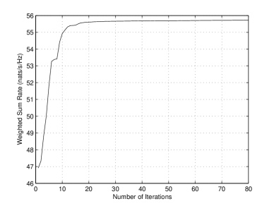
Figure 1: Convergence behavior of a 10-user MIMO-BC with $n_{t}=n_{r}=4$.

To compare the efficiency of CGP with that of IWFs, we give an example of an equal-weight large MIMO-BC system consisting of 100 users with $n_{t}=n_{r}=4$ in here. The convergence processes are plotted in Fig. 2. It is observed from Fig. 2 that CGP takes only 29 iterations to converge and it outperforms both IWFs. IWF1’s convergence speed significantly drops after the quick improvement in the early stage. It is also seen in this example that IWF2’s performance is inferior to IWF1, and this observation is in accordance with the results in [10]. Both IWF1 and IWF2 fail to converge within 100 iterations. The scalability problem of both IWFs is not surprising because in both IWFs, the most recently updated covariance matrices only account for a fraction of $1/K$ in the effective channels’ computation, which means it does not effectively make use of the most recent solution. In all of our numerical examples with different number of users, CGP always converges within 30 iterations.

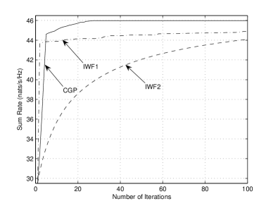
Figure 2: Comparison in a 100-user MIMO-BC channel with $n_{t}=n_{r}=4$.

VI Conclusion

In this paper, we studied the maximum weighted sum rate (MWSR) problem of MIMO-BC. Specifically, we derived the MWSR problem of the dual MIMO-MAC with a sum power constraint and developed an efficient algorithm based on conjugate gradient projection (CGP) to solve the MWSR problem. Also, we theoretically and numerically analyzed its complexity and convergence behavior. Our contributions in this paper are three-fold: First, this paper is the first work that considers the MWSR problem of MIMO-BC; Second, we simplified the MWSR problem in the dual MIMO-MAC and showed that enumerating all different decoding orders is unnecessary; Third, we developed an efficient and well-scalable algorithm based on conjugate gradient projection (CGP). The attractive features of CGP and encouraging results in this paper showed that CGP is an excellent method for solving the MWSR problem of large MIMO-BC systems.

References

• [1] T. M. Cover and J. A. Thomas, Elements of Information Theory.   New York-Chichester-Brisbane-Toronto-Singapore: John Wiley & Sons, Inc., 1991.
• [2] H. Weingarten, Y. Steinberg, and S. Shamai (Shitz), “The capacity region of the Gaussian multiple-input multiple-output broadcast channel,” IEEE Trans. Inf. Theory, vol. 52, no. 9, pp. 3936–3964, Sep. 2006.
• [3] S. Vishwanath, N. Jindal, and A. Goldsmith, “Duality, achievable rates, and sum-rate capacity of MIMO broadcast channels,” IEEE Trans. Inf. Theory, vol. 49, no. 10, pp. 2658–2668, Oct. 2003.
• [4] P. Viswanath and D. N. C. Tse, “Sum capacity of the vector Gaussian broadcast channel and uplink-downlink duality,” IEEE Trans. Inf. Theory, vol. 49, no. 8, pp. 1912–1921, Aug. 2003.
• [5] W. Yu, “Uplink-downlink duality via minimax duality,” IEEE Trans. Inf. Theory, vol. 52, no. 2, pp. 361–374, Feb. 2006.
• [6] J. Liu and Y. T. Hou, “Cross-layer optimization of MIMO-based mesh networks with gaussian vector broadcast channels,” Technical Report, Deptment of ECE, Virginia Tech, Mar. 2007. [Online]. Available: http://filebox.vt.edu/users/kevinlau/publications/
• [7] T. Lan and W. Yu, “Input optimization for multi-antenna broadcast channels and per-antenna power constraints,” in Proc. IEEE GLOBECOM, Dallas, TX, U.S.A., Nov. 2004, pp. 420–424.
• [8] H. Viswanathan, S. Venkatesan, and H. Huang, “Downlink capacity evaluation of cellular networks with known-interference cancellation,” IEEE J. Sel. Areas Commun., vol. 21, no. 5, pp. 802–811, Jun. 2003.
• [9] W. Yu, “A dual decomposition approach to the sum power Gaussian vector multiple-access channel sum capacity problem,” in Proc. Conf. Information Sciences and Systems (CISS), Baltimore, MD, U.S.A., 2003.
• [10] N. Jindal, W. Rhee, S. Vishwanath, S. A. Jafar, and A. Goldsmith, “Sum power iterative water-filling for multi-antenna Gaussian broadcast channels,” IEEE Trans. Inf. Theory, vol. 51, no. 4, pp. 1570–1580, Apr. 2005.
• [11] J. Liu, Y. T. Hou, and H. D. Sherali, “Conjugate gradient projection approach for multi-antenna gaussian broadcast channels,” in Proc. IEEE ISIT, Nice, France, Jun. 2007, to appear.
• [12] S. Ye and R. S. Blum, “Optimized signaling for MIMO interference systems with feedback,” IEEE Trans. Signal Process., vol. 51, no. 11, pp. 2839–2848, Nov. 2003.
• [13] M. S. Bazaraa, H. D. Sherali, and C. M. Shetty, Nonlinear Programming: Theory and Algorithms, 3rd ed.   New York, NY: John Wiley & Sons Inc., 2006.
• [14] J. R. Magnus and H. Neudecker, Matrix Differential Calculus with Applications in Statistics and Economics.   New York: Wiley, 1999.
• [15] S. Haykin, Adaptive Filter Theory.   Englewood Cliffs, NJ: Prentice-Hall, 1996.
• [16] J.-B. Hiriart-Urruty and C. Lemaréchal, Fundamentals of Convex Analysis.   Berlin: Springer-Verlag, 2001.