Geographic Routing Around Obstacles in Wireless Sensor Networks
Technical Report

Abstract

Geographic routing is becoming the protocol of choice for many sensor network applications. The current state of the art is unsatisfactory: some algorithms are very efficient, however they require a preliminary planarization of the communication graph. Planarization induces overhead and is not realistic in many scenarios. On the other hand, georouting algorithms which do not rely on planarization have fairly low success rates and either fail to route messages around all but the simplest obstacles or have a high topology control overhead (e.g. contour detection algorithms). To overcome these limitations, we propose GRIC [PN07], the first lightweight and efficient on demand (i.e. all-to-all) geographic routing algorithm which does not require planarization and has almost 100% delivery rates (when no obstacles are added). Furthermore, the excellent behavior of our algorithm is maintained even in the presence of large convex obstacles. The case of hard concave obstacles is also studied; such obstacles are hard instances for which performance diminishes.

Chapter 1 Introduction

We consider the problem of routing in ad hoc wireless networks of location aware stations, i.e. the stations know their location in a coordinate system such as the Euclidean plane. This problem is commonly called geographic routing (georouting for short). We are motivated by the case where the network is actually a wireless sensor network (sensor net) and we address the specific requirements imposed by their very stringent constraints. In particular, routing algorithms should be realistic and usable in real world scenarios, including urban scenario with large communication blocking obstacle (such as walls, buildings) and areas of low node density (sometimes called routing holes).

Problem definition.

The problem we are addressing is therefore to find a simple and efficient georouting algorithm delivering messages with high success rate even in the presence of large communication blocking obstacles and regions of low node density. The georouting algorithms we allow ourselves to consider should be lightweight, on demand, efficient and realistic.

Lightweight is notably understood in terms of topology maintenance overhead (our algorithm actually requires no link-layer topology maintenance), on demand means it should be all-to-all (as opposed to all-to-one and one-to-all algorithms) and not rely on storing any routing table, efficiency is measured in terms of success rate (the probability that a message reaches its destination) and hop-stretch (i.e. the path length should be short) and it should be realistic and of practical use for real world sensor nets, thus avoid relying on any unrealistic assumptions (such as unit disc graphs).

1.1 Background on Sensor Networks and Geographic Routing

Recent advances in micro-electromechanical systems (MEMS) and wireless networking technologies have enabled the development of very small sensing devices called sensor nodes [RAdS⁺00, WLLP01, ASSC02]. Unlike traditional sensors that operate in a passive mode, sensor nodes are smart devices with sensing, data-processing and wireless transmission capabilities. Data can thus be collected, processed and shared with neighbours. Sensor nodes are meant to be deployed in large wireless sensor networks (sensor nets) instrumenting the physical world. Originally developed for tactical surveillance in military applications, their are expected to find growing importance in civil applications such as building, industrial and home automation, infrastructure monitoring, agriculture and security. Their range of applications makes sensor nets heterogeneous in terms of size, density and hardware capacity. Their great attractiveness follows the availability of low cost, low power and miniaturized sensor nodes pervading, instrumenting and reality augmenting the physical world without requiring human intervention: sensor nets are self-organizing, self repairing and highly autonomous. Those properties are implemented by designing protocols addressing the specific requirements of sensor nets. Common to all sensor net architecture and applications is the need to propagate data inside the network. Almost every scenario implies multi-hop data transmission because of low power used for radio transmission mostly to limit depletion of the scare energy resources of battery powered sensor nodes. As a consequence, routing comes as a fundamental primitive of every full fledged sensor network protocol, whatever the application, the topology and the hardware composing the sensor net. Zhao and Guibas [ZG04] claim with purpose that routing protocols for sensor nets need to respond to specific constraints.

“The most appropriate protocols [for sensor nets] are those that discover routes on demand using local, lightweight, scalable techniques, while avoiding the overhead of storing routing tables or other information that is expensive to update such as link costs or topology changes”.

Geographic routing is a very attractive solution for sensor nets. The most basic georouting algorithm is the greedy georouting algorithm described by Finn [Fin87], where messages are propagated with minimization of the remaining distance to the message’s destination used as a heuristic for choosing the next hop relay node. Foundational (and some more advanced) georouting techniques and limitations are covered in most text books on sensor nets, e.g. [KW05, ZG04]. The greedy routing algorithm discovers routes on demand and is all-to-all (as opposed to all-to-one), it uses only location information of neighbour nodes, it scales perfectly well, requires no routing tables and adapts dynamically to topology changes. The only requirement, which is a strong one, is that sensor nodes have to be localized, i.e. they should have access to coordinates defining their position. The major problem of the greedy approach is that messages are very likely to get trapped inside of local minimums (nodes who have no neighbours closer to the destination than themselves). For this reason early georouting has received much attention and research, motivated by the gain in momentum of ad hoc wireless networking has been fruitful in inventing ingenious new georouting techniques which we review in more details in section 1.4.

1.2 Localization

How reasonable is it to assume that sensor nodes are localized? It is usually accepted that the use of GPS like technology on every node is not reasonable for sensor nets. Therefore, one may ask to what extent the strong hypothesis of localised nodes restricts the application of georouting techniques to a specialized niche of sensor nets. First of all, clearly localization of nodes comes at a cost, but this cost can be kept reasonable through the use of one of the localization techniques for sensor nets often using GPS like technology to localize a few beacon nodes followed by a distributed protocol to localise the bulk of sensor nodes as described in general books on sensor nets such as [KW05, Beu05, ZG04], recent papers such as [LMPR06] or in the extensive survey in [HB01]. Those techniques come at the price of an overhead in terms of protocol complexity which would diminish the attractiveness of georouting if it was not for the fact that in many application localization will be required anyway since, as explained by Karl and Willig [KW05]:

“…in many circumstances, it is useful and even necessary for a node in a wireless sensor network to be aware of its location in the physical world. For example, tracking or event-detection functions are not particularly useful if the [sensor net] cannot provide any information where an event has happened”.

As a consequence, georouting does not confine to a specialised niche but on the contrary it is becoming a protocol of choice for sensor nets as advocated by Seada, Helmy and Govindan [SHG04]:

“…[georouting] is becoming the protocol of choice for many emerging applications in sensor networks, such as data-centric storage [RKY⁺02] and distributed indexing [GEG⁺03]”.

We are therefore confident that georouting will be a sustainable approach for many sensor net applications and that the ongoing research will keep improving the state of the art to a point where localisation will be made available with high precision at low protocol overhead for sensor nets. Interestingly, it may be noticed that georouting can even be used when nodes are not localised by using virtual coordinates as was proposed in [RRP⁺03].

1.3 Our approach

To overcome the limitations of previous approaches, we propose a new algorithm called GRIC (GeoRoutIng around obstaCles) [PN07]. The main idea of GRIC is to appropriately combine movement directly towards the destination to optimize performance with an inertia effect that forces messages to keep moving along the “current” direction so that it will closely follow obstacle shapes in order to efficiently bypass them. In order to route messages around more complex obstacles we add a “right-hand rule” inspired component to our algorithm, which is borrowed from maze solving algorithms (algorithms one can use to find he’s way out of a maze). The right-hand rule is a well known “wall follower” technique to get out of a maze [Hem89] which has been previously used by some of the most successful georouting algorithms known so far (c.f. section 1.4). However, whereas previous algorithms used a strict implementation of the right hand rule we only inspire ourselves from it. The reason is that the right-hand rule, originally developed to find a path out of a maze, only works for planar graphs but we want to ensure that GRIC runs on the complete (non planarized) communication graph.

1.3.1 Methodology

We implement our algorithm and comparatively evaluate its performance against those of other representative algorithms (greedy, LTP, and face routing). We focus on three performance measures: success rate, distance travelled and hop count. We study the impact on performance of several types of obstacles (both convex and concave) and representative regimes of network density.

1.3.2 Comparison

When compared to other georouting algorithms, GRIC features no topology maintenance overhead, practical usefulness in the sense that it runs on real world complete (directed) communication graphs and is capable of routing messages to their destination with high success rate, even in the presence of large communication blocking obstacles. The combination of those features makes GRIC unique. Some previous algorithms had high success rates, however none of them works on directed communication graphs and they all suffer either from a high topology maintenance overhead or are not practical because requiring the unrealistic assumption that the communication graph is (almost) a unit disc graph. Other algorithms are lightweight (i.e. have low topology maintenance overhead), but none of them has competing success rates when compared to GRIC , furthermore none of them is capable of routing messages around large obstacles.

1.3.3 Strengths of our approach:

Our algorithm has the advantage of being many-to-many and on demand, i.e. no routing tables have to be stored, no flooding is required to establish a gradient and no interests have to be propagated for the routing to be successful. This is possible because the nodes are localised and arguably is part of the strengths inherent to all georouting algorithms. It is in large part responsible for the attractiveness of this kind of protocols.

Our algorithm seems to somehow combine the best of two worlds. In terms of algorithm design, it combines the light weight and simplicity of the greedy type of algorithms while avoiding the (sometimes unrealistic and high topology maintenance overhead) topology maintenance phase (usually planarization) required by the GFG [BMSU99] and GPSR [KK00] algorithms and their successors. c.f. section 1.5.1 for a detailed explanation of the limitations induced by the planarization phase. In terms of performance, our findings demonstrate that in most cases our algorithm outperforms the previous ones. Furthermore, its performance with respect to the path length is very close to the length of an optimal path in the case of no global knowledge, e.g. when the presence of obstacles is not known to the algorithm in advance but only sensed when reaching the obstacles. It may also be worth pointing out that our algorithm seems to be resistant to temporary link failure, as suggested by the fact that the randomized version of GRIC actually performs better than the deterministic one, c.f. section 2.3.7 Because our algorithm is the first lightweight algorithm to efficiently bypass large and complex obstacles without requiring a preliminary planarization phase, we feel it considerably advances the current state of the art for gerouting algorithms.

1.4 Related Work

The major problem of the early greedy geometric routing algorithms [Fin87] is the so called routing hole problem [KW05, ZG04, AKJ05] where messages get trapped by “local minimum” nodes which have no neighbours closer to the destination of the message than themselves. The incidence of routing holes increases as network density diminishes and the success rate of the greedy algorithm drops very quickly with network density. So far, georouting protocol have mainly focused on increasing the success rate (the probability that a message is successfully routed) while keeping the “lightweight” advantages of the greedy type of routing algorithms, although recent research efforts have also been proposed to deliver efficient georouting algorithms with respect to other metrics [SD04, KNS06]. Most georouting algorithms can be divided into two groups. On the one hand, those that guarantee delivery (i.e. the success rate is 100% if the communication graph is connected) [BMSU99, KK00] and probabilistic approaches that achieve certain performance trade-offs, such as [CDNS04, CDNS06, CNS02, CNS05, KNS06]. Alternatively, it is also possible to run topology discovery algorithms to discover routing holes and obstacles and to use this information to route messages around them. An example is the BOUNDHOLE algorithm from [FGG06] which uses the TENT rule to discover local minimum nodes and then to “bound” the contour of routing holes. The disadvantage of this type of approach is the heavy overhead and the fragility towards unstable topology (such as mobility of nodes). Although it has a very high overhead when compared to the algorithm we propose, the information gained during the contour discovery phase may be used for other application than routing such as path migration, information storage mechanisms and identification of regions of interest [FGG06].

1.5 Routing with Guaranteed Delivery

Arguably, most georouting algorithms are inspired by the routing protocols with guaranteed delivery from [BMSU99, KK00]. Those two protocols are almost similar and were, to our knowledge, developed independently. They consist of using a greedy routing algorithm until the message gets trapped in a routing hole. When the message gets trapped in the routing hole, the algorithm switches to a rescue mode until it is judged that switching back to greedy mode is appropriate. The rescue mode routes messages according to the face algorithm described by Prosenjit et al. [BMSU99] on a planar subgraph of the communication graph. The face algorithm improves on the compass-II routing algorithm from [KSU99]: the length of the path along which messages are routed by face is smaller than for compass-II. In [BMSU99] the FACE algorithm is used on the Gabriel subgraph of the complete communication graph, whereas in [KK00] the comparable relative neighbourhood graph is used . Further work proposes to optimize the switching mechanism between greedy and rescue mode [KWZ03, KWZZ03] in order to diminish the length of the routing paths. Face routing, is very attractive because it guarantees delivery, however it involves a number of issues. The most important issue is the fact that it requires a preliminary planarization phase, a procedure which may not be achievable in many realistic scenarios. Other issues include topology maintenance overhead, strong dependency on the unit disc graph model, sensitivity to localisation errors, increased path length, requirement of symmetric links and limitation to 2-dimensional networks. Because they motivate our present work, we include in section 1.5.1 a detailed comment on those issues, as well as some of the ways they have been (or not) addressed in previous works.

1.5.1 Issues with face routing

First of all, FACE has a clear topology maintenance overhead since the Gabriel graph has to be maintained at all times. This overhead is computationally reasonable since the Gabriel graph can be computed by a fully distributed algorithm [BMSU99]. A critical issue is the fact that, as acknowledged in [BFNO03], …the Gabriel graph that is used for routing is not a robust structure. The problem is that the FACE family of protocols assume that the communication graph is a random geometric graph built using the unit disc graph model. Whereas the unit disc graph model is commonly used to model wireless sensor networks for simulation purposes, the fact that it only approximates real world communication graphs for sensor networks is usually not a critical issue. On the contrary, the correctness of the FACE algorithm requires the communication graph of a real sensor network to be very close to a unit disc graph. This hypothesis may be very hard to match in practise and as shown in the micro-analysis of [SHG04] it results in non-recoverable errors for FACE like algorithms. One of the reason is that the hypothesis that sensor nodes can communicate to neighbour nodes if and only if their distance is beyond a given threshold is not true in real networks. See, for example [ZHKS04] for a study of radio irregularity in sensor networks. In [BFNO03], it is proposed to introduce virtual edges to overcome this problem. At the cost of introducing a little more topology maintenance overhead, they show that FACE is still usable in the case where the communication graph is a disc graph defined using two radius $r$ and $R$ (a “two radius” unit disc graph) with $r\leq R$ such that the ratio $\frac{R}{r}$ is smaller than $\sqrt{2}$. In the communication graph considered by [BFNO03] sensor nodes can always communicate to neighbours when their distance is smaller than $r$, can never communicate when their distance is greater than $R$, and communication is uncertain when the distance between them is between $r$ and $R$. Although this model is a generalisation of the unit disc graph model and the findings of [BFNO03] shows limited robustness of the Gabriel graph extraction algorithm permitting successful use of FACE, it is unclear how the two radius unit disc graph hypothesis will be matched in real sensor networks, although it will probably not be the case in many scenarios, as shown by recent work, c.f. section 1.5.2.

Yet another problem follows from localization imprecision of the nodes. [SHG04] show that even small localisation errors of $10\%$ of the transmission range have a great impact on the success rate of GPSR, which is a combination of greedy and FACE routing (on the contrary, it is shown in [HHB⁺03] that greedy is less affected by this problem). After acknowledging the problem, [SHG04] proposes a fix, called the mutual witness extension to GPSR, which seems to restore almost perfectly the excellent behavior of GPSR that is known to hold under the idealistic assumption that nodes have access to exact location information.

Furthermore, as acknowledged in [SD04], the FACE algorithm runs on a planar subgraph who’s construction favors short edges over long ones. The path length, which is a common measure of quality for routing algorithms is thus fairly long for the FACE algorithm. Early fall-back to greedy mode [BMSU99, KK00, KWZ03, KWZZ03] is one solution to this problem. Another solution is to use “shortcuts”, introduced in [DSW04] to reduce the path length of FACE. Obviously all those techniques are employed at the cost of an extra overhead in terms of topology maintenance of the communication graph.

Another limitation of FACE is that it will totally fail in the case where communication links are asymmetric. This could be a severe limitation for some otherwise simple and efficient energy aware optimisation schemes for routing algorithms (e.g. temporarily removing links to nodes with low energy and favoring links leading to motes with high remaining energy would create an asymmetric communication graph even if the original communication graph was symmetric). Even some otherwise efficient energy aware optimisation schemes may not be applicable to FACE, more subtle (and more complicated) approaches are still possible, like the proposition in [SD04] to favor next hop transmission to motes with high available energy in combination with the “shortcut” idea from [DSW04]. Roughly speaking, instead of choosing the shortcut that minimises the path length, a shortcut leading to a node with high remaining energy is chosen in combination with the use of a dominating subset of nodes to act as a backbone network for routing.

Finally, it may be noticed that FACE georouting is not applicable in the case of 3-dimensional networks, which may be a limitation for some applications of sensor networks.

1.5.2 Recent Progress Towards Realistic Guaranteed Delivery

As explained in the previous section, until recently the state of the art for georouting had a major flaw: it strongly depended on the assumption of a unit disc communication graph, thus making in unrealistic for many real world scenario. Very recently, Kim et Al. [KGKS05b] acknowledged this fact by presenting a series of pitfalls associated with geographic routing which extends and deepens the micro-analysis of [SHG04]. In a breakthrough paper [KGKS05a], the same authors propose the cross-link detection protocol (CLDP), the first face routing algorithm that works for arbitrary communication graphs, thus making geographic face routing practical in the sense that their algorithm works for real world wireless networks whose communication graphs do not need to resemble idealistic unit disc communication graphs. In fact, the algorithm works for any graph as long as the links are bi-directional, i.e. the communication graph is symmetric. The major drawback is that their solution, while becoming practical for real-world nets, induces a very high topology maintenance overhead in terms of message exchange in order to construct a subgraph of the complete communication graph. In order to reduce the communication overhead, Leong et Al. propose Greedy Distributed Spanning Tree Routing (GDTSR), a georouting algorithm [LLM06] reducing the communication overhead by orders of magnitudes. Their contribution has the originality of considering a new way of routing messages while in rescue mode, i.e. as a replacement to face routing. They propose to use convex-hull spanning trees. Although elegant, their solution requires building a few complex tree structures. To be made completely practical their solution would requires handling many tedious problems (such as selecting the roots of the trees or making the algorithm robust in case some nodes fails during the set-up phase). Therefore, their algorithm is far from being simple (it requires the study of subproblems and implementing solutions to those problems). Those difficulties affect the robustness of a complete protocol stack (MAC/data-link) implementation of their algorithm and even if those problems were being addressed the message overhead, although being reduced when compared to the solution in [KGKS05a], is still far from being insignificant. As a sign that those contributions are probably going to open a new area of creative improvements to georouting, Kim et Al. recently deepened [KGKS06] even further the understanding of the pitfalls of face georouting and, using a lazy cross-link removal (LCR) algorithm propose a practical face routing algorithm with significantly lower topology maintenance overhead than their previous proposition from [KGKS05a]. Nevertheless, the overhead is still significant, bi-directional links are still required and the knowledge of two hops away neighbours is required, which may be a limitation in case of highly dynamic networks.

1.6 Probabilistic approaches:

Guaranteed delivery algorithms have received plenty of attention in the literature because, when applicable, they are very powerful algorithms. A taxonomy of georouting algorithms is provided in [Sto02], focusing on guaranteed delivery but with a review of many other solutions. Some other solutions include the PFR [CDNS04, CDNS06], VTRP [ACM⁺04], the LTP protocols [CNS02, CNS05] or the CKN protocol from [CKN06]. Those protocols employ randomization and do not guarantee delivery, however they are more “lightweight” than the FACE type of algorithms and may also apply in a more general context than localised network. What is more, they do not require a planarization phase: they run on the full communication graph. PFR is a probabilistically limited flooding algorithm (it is thus multi-path), VTRP proposes to use variable transmission range capable hardware to bypass routing holes in low density areas and LTP is a combination of a modified greedy algorithm with limited backtracking as a rescue mode. The effect of obstacles on those three protocols was studied in [CMN06] and therefore provides a comparison to the GRIC algorithm proposed in this report. One of the results in [CMN06] is that all three protocols fail in the case of the stripe obstacle, which is the easiest obstacle considered in this report. In terms of obstacle avoidance, GRIC thus prevails over PFR, VTRP and LTP (as well as over all other “lightweight” georouting algorithms we know of). In the case of no obstacle, we shall show that GRIC is more efficient than LTP (and therefore than PFR, as follows from results in [CMN06]). VTRP is more efficient than GRIC in the case of networks of very low densities with no obstacles, but this is because VTRP uses additional hardware properties, namely, it “jumps over” routing holes by augmenting the transmission range when faced with a blockage situation. Although very nice when applicable, it may be noticed that this solution requires additional hardware capabilities, makes the protocol more complicated (since the MAC and link layer protocol have to adapt, for example neighbourhood discovery may have to be restarted for the new transmission range) and does not work if the obstacle is “physical”, in the sense that transmission range is blocked (i.e. it only deals with areas of low node density: routing holes). More recently, [CKN06] proposes a routing protocol that implicitly copes with simple obstacles and node failures by “learning”, i.e. gaining limited local knowledge of the actual network conditions, and by using this information to optimize data propagation. By planing routes a few hops ahead and by varying the transmission range it can therefore bypass routing holes (i.e. areas of low density but through which radio transmission is possible if the transmission range is increased) and some very simple obstacles. However, increasing the transmission range does not bring any improvement in the case of physical obstacles (through which radio propagation is impossible) or large obstacles which can not be “jumped over” by increasing the transmission range.

Chapter 2 The GRIC Algorithm

2.1 Sensor Network Model

This section describes the sensor net model we assume in this work. The assumptions we make are fairly weak and general. We consider sensor networks deployed on a two dimensional surface and we allow messages to piggy-back $\mathcal{O}(1)$ bits of information which is being used for the decision making of our routing algorithm (in fact, the only required information is the position of the last node visited by the message, the position of the final destination of the message and the value of a mark-up flag, c.f. section 2.3). The most important part of the model is the communication model. We assume that each node is aware of its own position, has access to the list of its outbound neighbours and to their positions, and that it can reliably send messages to its neighbours, i.e. GRIC runs on a directed communication graph where nodes are localised and aware of their neighbours as well as their positions. This combinatorial model is reasonable and realistic for sensor nets. Indeed, our GRIC algorithm is a network layer algorithm. The network layer relies on an underlying data link layer which in turn relies on a MAC and physical layer. Real world sensor networks implementation of our algorithm would therefore have to implement all levels of the protocol stack, and it is reasonable to assume that the link layer provides the level of abstraction required by our algorithm. We discuss in more details a realistic and simple full layer implementation of our algorithm (including physical, MAC and data link layers) in the next section.

2.2 Lower Layers of the Protocol Stack

For completeness we discuss the assumptions we make for every layer upon which the network layer relies: the physical, the MAC and the link layers.

Because our algorithm situates itself at the network layer level, it is not strongly dependant on the physical layer, i.e. the type of nodes. Highly limited piconodes forming very large smart dust nets [ASSC02, WLLP01, EGHK99] composed of nodes smaller than a cubic centimeter, weighting less than 100 grammes and with costs well under a dollar such as envisioned in [RAdS⁺00, WLLP01] but with probably strong limitations in terms of resource and features are perfectly acceptable. On the other hand more reasonable sensor nodes proposed by OEM nowadays are fine too. Those nodes are typically the size of a matchbox (including battery) and with a cost of more than a hundred dollars. We assume that each sensor node is a fully-autonomous computing and communicating device, equipped with a set of sensors (e.g for temperature, motion, or metal detector). It has a small CPU, some limited memory and is strongly dependant on its limited available energy (battery). Each sensor can communicate wireless with other sensors of the network which are within communication range. We do not assume that sensor nodes can vary their transmission range.

We assume that a MAC layer protocol such as the S-MAC protocol from [YHE02] or an IEEE 802.11-like MAC protocol is running on each sensor node. The MAC layer protocol is in charge of neighbourhood discovery and it provides the link layer protocol with a list of neighbours with which the sensor node is capable of symmetric communication.

At the link layer, we assume a protocol that provides each node with a list of reliable outbound wireless communication links (i.e. at the link layer we do not need to assume the communication link to be symmetric, which is a feature of our algorithm). This means that the link layer protocol can remove some of the links provided at the MAC layer (e.g. those links which cannot be made reliable at reasonable costs, for example by including some quality metric on the links).

Georouting algorithms all make a further assumption: sensor nodes are localised for example using one of the currently available localisation techniques [Beu05, ZG04, KW05, HB01]. We assume that the link layer protocol adds this information to the list of links: the position of the sensor to which messages are sent if a given wireless link is chosen.

Our GRIC routing protocol situates itself at the network layer. It runs on each individual node and the input to the algorithm is the position of the node on which it runs, as well as the list of links (including the position of the node to which those links lead to) provided by the link layer protocol.

GRIC is assumed to be capable of reliably sending messages to any of its outbound neighbour. The reliability issue (collision avoidance, acknowledgments, etc) is not taken into account by GRIC but by the lower layer protocols (link layer and MAC layer). Reliable transmission can be achieved through many possible techniques, like time division multiple access schemes (TDMA) at the MAC layer, acknowledgement with retransmission or error correcting codes at the data-link layer or, alternatively multipath redundancy could be added on top of GRIC. Because many different options exist, our assumption of reliable communication links is realistic but out of the scope of the current report.

2.3 Algorithms

Like the FACE family of algorithms and their successors [BMSU99, KK00, KWZ03, KWZZ03], GRIC (GeoRoutIng around obstaCles) [PN07] uses two different routing modes: a normal mode called inertia mode and a rescue mode called contour mode. The inertia mode is used when the message makes progress towards the destination, and the contour mode when it is going away from the destination. The two major ingredients which make our approach successful is the use of the inertia principle and the use of the so called right-hand rule. The inertia principle is borrowed to physics and we use it to control the trajectory of messages inside the network. Informally, messages are “attracted” to their destination (like a celestial body is attracted in a planet system) but have some inertia (i.e. they also have an incentive to follow the “straight line”). The right-hand rule is a “wall follower” technique to get out of a maze [Hem89] and we use it to route messages around complex obstacles. We use this informal idea to ensure that messages follow the contour of obstacles. The successful implementation of both of these abstract principles uses a virtual compass device (described in section 2.3.2) which treats a message’s destination as the north pole. The compass device, the inertia principle and the right-hand rule enables the computation of an idealistic direction in which the message should be sent (c.f. figure 2.1). Since there may not be a node in this exact direction, the message is actually sent to the mote maximizing progress towards the ideal direction.

2.3.1 Routing with inertia:

In this section, we give a high level description of the inertia routing mode. Intuitively, the inertia mode performs greedy routing with an adjunct inertia conservation parameter $\beta$ ranging in $\left[0,1\right]$. When a node routes a message in inertia routing mode, it starts by computing an ideal direction vector $v_{\textrm{ideal}}$. Once this ideal direction vector is computed, the message is sent to the node maximizing progression in the ideal direction. We next describe how to compute $v_{\textrm{ideal}}$ and how to choose the node with best progression towards the ideal direction. To compute the ideal direction, the routing node needs to know its own position $p$, the position $p^{\prime}$ of the node from which the message was received and the position $p^{\prime\prime}$ of the message’s destination, c.f. figure 2.1(a) below.

(a) Ideal direction.

(b) The compass returns NW.

Figure 2.1: Computation of the ideal direction and the compass device.

The position $p^{\prime}$ is assumed to be piggy-backed on the message, therefore, access to $p$, $p^{\prime}$ and $p^{\prime\prime}$ is consistent with the sensor network model described in section 2.1. First, the node $p$ computes $v_{\textrm{prev}}=\overrightarrow{p^{\prime}p}$, which is a vector pointing in the last direction travelled by the message, as well as $v_{\textrm{dest}}=\overrightarrow{pp^{\prime\prime}}$, which is a vector pointing in the direction of the message’s destination. Through elementary trigonometry an angle $\alpha$ is computed, such that $\alpha$ is the unique angle in $\left[-\pi,\pi\right[$ with $\mathcal{R}_{\alpha}\cdot v_{\textrm{prev}}^{\top}=v_{\textrm{dest}}^{\top}$, where $v^{\top}$ denotes vector transposition and where $\mathcal{R}_{\alpha}$ is the following rotation matrix:

$$\mathcal{R}_{\alpha}=\left(\begin{array}[]{lr}\cos(\alpha)&-\sin(\alpha)\\ \sin(\alpha)&\cos(\alpha)\end{array}\right)$$

The node can now compute the ideal direction in which to send the message. For the inertia mode, the ideal direction is defined as $v_{\textrm{ideal}}=\mathcal{R}_{\alpha^{\prime}}\cdot v_{\textrm{prev}}$, where $\mathcal{R}_{\alpha^{\prime}}$ is a rotation matrix with $\alpha^{\prime}$ defined by

$$\begin{array}[]{lccl}\alpha^{\prime}&=-&\beta\pi&\textrm{ if }\alpha<-\beta\pi,\\ \alpha^{\prime}&=&\beta\pi&\textrm{ if }\alpha>\beta\pi,\\ \alpha^{\prime}&=&\alpha&\textrm{ otherwise}\end{array}$$

The ideal direction $v_{\textrm{ideal}}$ is thus obtained by applying a rotation to the previous direction $v_{\textrm{prev}}$ towards the destination’s direction $v_{\textrm{dest}}$, however, the maximum rotation angle allowed is bounded, in absolute value, by $\beta\pi$. This implies that the ideal direction is somewhere in between the previous direction and the direction of the message’s destination.

Remark.

To enhance intuitive understanding of the inertia routing mode, it may be useful to notice that setting $\beta=1$ implies that $v_{\textrm{ideal}}=v_{\textrm{dest}}$. In other words the ideal direction is always towards the message’s destination and inertia routing is equal to the simple greedy geometric routing. At the other extreme, setting $\beta=0$ implies that $v_{\textrm{ideal}}=v_{\textrm{prev}}$, i.e. the message always tries to go straight ahead: there is maximal inertia. In our simulations, setting $\beta=\frac{1}{6}$ proved to be a good choice for practical purposes.

After the ideal direction has been computed the message is sent to the neighbour maximizing progress towards the ideal direction. Maximal progress is defined to be reached by the node $m$ (amongst outbound neighbours of the node currently holding the message) such that $\textit{progress}(m):=\left<v_{\textrm{ideal}}|\textit{pos}(m)-p\right>$ is maximized, where $\left<\cdot|\cdot\right>$ is the standard scalar product and $\textit{pos}(m)$ is the position of $m$.

Inertia routing is already quite an improvement over simple greedy routing, as can be seen on figure 2.2(a) where a message is successfully routed from a point $a=(0,10)$ to a point $b=(20,10)$ in the presence of an obstacle (a stripe).

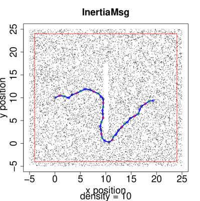
(a) Success.

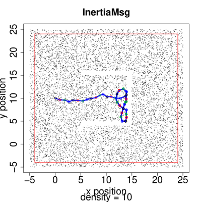
(b) Failure.

Figure 2.2: Inertia routing with two different obstacles.

We delay detailed explanations of the simulation context in which the plots of figure 2.2 where obtained. Our intention in showing figure 2.2 now is to show that although inertia routing successfully avoids a simple obstacle (the stripe of figure 2.2(a)), it fails for the more complicated U shape obstacle of figure 2.2(b) (more details will be given in section 3.1). This routing failure is the motivation for adding a contour mode to which our algorithm can switch when it needs to route messages around complicated obstacles.

2.3.2 Routing around obstacles:

We will now describe the contour mode of our algorithm, as well as the mechanism which permits to switch between contour mode and inertia mode. The contour mode, as well as the switching mechanism both make use of a virtual compass indicating the direction travelled by the message during its last hop relatively to its final destination.

2.3.3 The compass device:

When a node generates a message, we take the convention to say that the message has traveled its last hop towards the north. Otherwise, we use the points $p$, $p^{\prime}$ and $p^{\prime\prime}$ to compute the angle $\alpha$ between the last direction travelled by the message $v_{\textrm{prev}}$ and the direction to the message’s destination $v_{\textrm{dest}}$ as was done in section 2.3.1, c.f. figure 2.1. Seeing $v_{\textrm{dest}}$ as the north, the virtual compass device returns a value in north-west, north-east, south-west and south-east depending on the quadrant in which $\alpha$ lies: SW if $\alpha\in\left[-\pi,-\pi/2\right[$, NW if $\alpha\in\left[-\pi/2,0\right[$, NE if $\alpha\in\left[0,\pi/2\right[$ and SE otherwise. See figure 2.1(b) for an intuitive explanation of the compass device, while a a rigorous description of the computation steps implementing the virtual compass is given in procedure 1 (compass).

Procedure 1 Compass

  $v_{\textrm{last}}\leftarrow\overrightarrow{p^{\prime}p}$

  $v_{\textrm{north}}\leftarrow\overrightarrow{pp^{\prime\prime}}$

  $\alpha\leftarrow angle\_from\_to(v_{\textrm{prev}},v_{\textrm{dest}})$

  if  $\alpha\in\left[-\pi,-\pi/2\right[$ then

     return  SW

  else if  $\alpha\in\left[-\pi/2,0\right[$ then

     return  NW

  else if  $\alpha\in\left[0,\pi/2\right[$ then

     return  NE

  else {Comment: in this case $\alpha\in\left[\pi/2,\pi\right[$}

     return  SE

Procedure 2 Mode Selector

  if  the flag is up then

     if the flag is tagged with E and $\texttt{compass}\in\left\{\texttt{NW},\texttt{SW}\right)$ then

        return  contour mode

     else if  the flag is tagged with W and $\texttt{compass}\in\left\{\texttt{NE},\texttt{SE}\right\}$)  then

        return  contour mode

  else

     return  inertia mode

2.3.4 The right and left hand rules to route around obstacles

The inertia routing mode manages to route messages around some simple obstacles, but not around more complicated obstacles. In order to improve it, we need to detect when a message is trying to go around an obstacle and switch to the contour mode when appropriate. The main idea in our contour mode is to choose either the right-hand rule or the left-hand rule, and to go around the obstacle according to this rule. The right-hand rule means that the message will go around the obstacle by keeping it on its right. When a node receives a message, it makes a call to the compass procedure to get the direction of the message and uses a flag which is piggy-backed on the message to decide if the right-hand rule (or the left-hand rule) should be applied. If the flag is down, the algorithm looks at the compass. If the compass points to the north, nothing special is done (it means the message is making progress towards its destination, and we stay in the inertia mode). But if the compass points south, it means that the message is actually going away from its destination, and the algorithm interprets this as the fact that the message is being routed around an obstacle. To acknowledge this fact, GRIC raises the contour flag and tags it with E or W if the compass points to the south-east or the south-west respectively. Once the flag is up, the message is considered to be trying to go around an obstacle using the right-hand rule or the left-hand rule if the flag is tagged W or E respectively. See procedure 3 (raise flag) for a detailed explanation.

Procedure 3 Raise flag (Raise and Mark the Flag)

  {By assumption the flag is down}

  if Compass == SW then

     Raise flag

     Tag flag with the W value

  else if Compass == SE then

     Raise flag

     Tag flag with the E value

  else

     Let the flag down

Once the message is considered to be trying to go around an obstacle using the right-hand rule (i.e. if the flag is up and tagged W,), the algorithm will not change its mind until the message reaches a node where the compass returns the value NW (or NE if the left-hand rule was used). See procedure 4 (lower flag) for a rigorous description.

Procedure 4 Lower Flag

  {By assumption the flag is up}

  if  ( flag is tagged with W and compass == NW ) then

     put the flag down

  else if  ( flag is tagged with E and compass == NE ) then

     put the flag down

  else

     Let the flag up and don’t change the tag

To summarize our discussion so far, when a node receives a message two different cases may occur: either the flag is down or it is up. If the flag is down (the message is not currently trying to go around an obstacle), GRIC runs procedure 3 (raise flag) to see if the message has just started going around an obstacle and flag and tag it appropriately. On the other hand, if the flag is up, it means the message was going around an obstacle, the procedure 4 (lower flag) is used to see if the message should be considered as having finished going around the obstacle and the flag can be brought down. The position of the flag, together with the position of the compass is used to determine if the message is to be routed according to the inertia or the contour mode.

2.3.5 Mode selection

The flagging mechanism described in the previous section enables a node to know if a message is being routed around an obstacle by looking at the position of the flag (which is piggy-backed on the message). When the flag is down, the inertia mode is used. However, when the flag is up, the contour mode (which we shall describe below) may have to be used. We next describe informally the mechanism used to decide whether the contour mode or normal mode should be used when the flag is up. Therefore, suppose the flag is up, and in order to simplify the discussion, suppose it is tagged with the E value (if the tag is W, a symmetric case is applied). Note that by case assumption, this implies that the compass either returned NW, SW or SE, since otherwise procedure 4 (lower flag) would have put the flag down. The message is therefore currently trying to go around an obstacle using the left-hand rule described in the previous section, trying to keep the obstacle on its left. Two different cases have to be considered. In the first case, the compass points SE. Recalling the definition of the ideal direction $v_{\textrm{ideal}}$ and of the previous direction $v_{\textrm{prev}}$ from section 2.3.1, it is easy to see that since by case assumption the compass points to south-east, $v_{\textrm{ideal}}$ is obtained by applying to $v_{\textrm{prev}}$ a rotation to the left (i.e. counter-clockwise), which is equivalent to saying the angle $\alpha$ defined in section 2.3.1 takes a value in $\left[0,\pi\right]$ and therefore that the angle $\alpha^{\prime}$ takes a value in $\left[0,\pi/6\right]$). In other words, the inertia routing mode tries to make the message turn left, which is consistent with the idea of the left-hand rule: routing the message along the perimeter of the obstacle while keeping it to the left of the message’s path. There is therefore no need to switch to the rescue contour mode. The second case which may occur is when the compass points either to the SW or to the NW. A similar reasoning to the previous one show that in this case the inertia routing mode will make the message turn right and the angle $\alpha^{\prime}$ will be in $\alpha^{\prime}\in\left[-\pi/6,0\right]$. According to the left-hand rule idea, the obstacle should be kept on the left of the message, however turning right, according to the inertia routing mode, will infringe the idea of keeping the obstacle to the left. Instead, the message would turn right and get away from the perimeter of the obstacle. In this case, it is therefore required to call the rescue mode: the contour mode. Rigorous description of the above discussion is given in procedure 2 (mode selector).

2.3.6 The contour mode

By case assumption, the flag is up. We also suppose without loss of generality that the tag on the flag is E, since the case of a W tag is similar. We have seen that procedure 2 (mode selector) calls the contour mode when the inertia mode is going to make the message turn right (or left if the tag is W), which is equivalent to saying that $\alpha\in\left[-\pi,0\right]$ and $\alpha^{\prime}\in\left[-\pi/6,0\right]$. However, the left-hand rule would advice turning on the left to stay as close as possible to the obstacle and to keep it on the left of the message path. Therefore, in order to stay consistent with the left-hand rule idea, we define $\alpha_{2}=-\textit{sign}(\alpha)(2\pi-\left|\alpha\right|)$, thus $\alpha_{2}$ is an angle such that $\textit{sign}(\alpha_{2})=-\alpha$ and such such that $R_{\alpha_{2}}\cdot v_{\textrm{prev}}^{\top}=R_{\alpha}\cdot v_{\textrm{prev}}^{\top}=v_{\textrm{prev}}^{\top}$. In order to give some inertia to the message we define $\alpha_{2}^{\prime}$ from $\alpha_{2}$ in a similar way as $\alpha^{\prime}$ was defined from $\alpha$, and the ideal direction $v_{\textrm{ideal}}$, is defined by $v_{\textrm{ideal}}^{\top}=R_{\alpha_{2}^{\prime}}\cdot v_{\textrm{prev}}^{\top}$, where $\alpha_{2}^{\prime}=\beta\alpha_{2}$, where $\beta$ is the inertia conservation parameter of section 2.3.1. Putting all things together, GRIC is formally described by the (non-randomized version of) algorithm 1.

Algorithm 1 GRIC , running on the node $n$ which is at position $p_{n}$.

1:  if the flag is down then

2:     call Raise flag {Procedure 3}

3:  else

4:     call Lower flag {Procedure 4}

5:  $mode:=\texttt{\bf{Mode selector}}$ {Procedure 2 }

6:  if  $mode==\textit{inertia mode}$  then

7:     $\gamma:=\alpha^{\prime}$ {Where $\alpha^{\prime}$ is the angle defined in section 2.3.1}

8:  else

9:     $\gamma:=\alpha_{2}^{\prime}$ {Where $\alpha_{2}^{\prime}$ is the angle defined in section 2.3.2}

10:  $v_{\textrm{ideal}}^{\top}:=R_{\gamma}\cdot v_{\textrm{prev}}^{\top}$

11:  Let $\mathcal{V}$ be the set of neighbours of $n$.

12:  if running the non-random version of GRIC  then

13:     Send the message to the node $m\in\mathcal{V}$ maximizing $\left<v_{\textrm{ideal}}|\overrightarrow{p_{n}p_{m}}\right>$, where $p_{m}$ is the position of $m$.

14:  else if running the random version of GRIC  then

15:     Let $\mathcal{V^{\prime}}$ be an empty set.

16:     for all  $v\in\mathcal{V}$  do

17:        add $v$ to $\mathcal{V^{\prime}}$ with probability $0.95$

18:     Send the message to the node $m\in\mathcal{V^{\prime}}$ maximizing $\left<v_{\textrm{ideal}}|\overrightarrow{p_{n}p_{m}}\right>$, where $p_{m}$ is the position of $m$.

2.3.7 Randomization

We shall show experimentally that GRIC succeeds in routing messages around local minimum and around obstacles with high probability (where the probability is taken over randomly generated networks). However, in unfavorable cases it may fail. We observed experimentally that adding a small random disturbance to the GRIC algorithm improves its behavior. Intuitively, if the message gets blocked in a local minimum and starts looping, a small random perturbation may be sufficient to make the message escape the routing loop. Instead of considering $\mathcal{V}$ to be the set of neighbours of $n$, we consider $\mathcal{V}$ to be the subset of neighbours of $n$ where each neighbour is added to $\mathcal{V}$ with probability $1-\epsilon$, where $\epsilon$ is a small constant. For practical purposes experiments have shown the choice of $\epsilon=0.05$ to be good. Formally, this idea is implemented by introducing the if-else cases on lines 12 and 14 of algorithm 1 to differentiate between random and non-random routing modes. It may be worth noticing that the random version of GRIC could also be interpreted as simulating temporary link failure in the network. This point of view implies that GRIC is actually robust to limited link failure.

Chapter 3 Experiments

3.1 Methodology

Our methodology is the following. We abstractly design a simple experiment which consists of (1) deploying a sensor net, (2) generate a message which has to be routed from a point $a$ to a point $b$ of the network and (3) measure the outcome of the experiment (successful or failed message delivery and efficiency of the routing path found by our algorithm, but c.f. details below). Running experiments on a real sensor network has a high cost (sensor nodes are still prohibitively expensive to run large scale experiments) and even if using a small scale real sensor network, running enough experiments to have statistically meaningful results would be extremely time consuming and probably unrealistic in the design phase of the algorithm. For those reasons, we decide to use “in silico” simulations to validate our sensor network algorithm which we describe below. A single simulation consists of deploying sensor nodes randomly and uniformly in a square region $\mathcal{R}$ of $30\times 30$ unit length sides and routing a message from the point $a=(10,0)$ to the point $b=(20,0)$ (c.f. figures 3.2(a) to 3.2(d)).

3.1.1 Simulation Platform and Model

For computational efficiency of our simulation platform, we use a high level simulation of a sensor network. In particular, we do not simulate the physical, the MAC and the network layer of the sensor network, but use the unit disc graph combinatorial model of a real world communication graph. In this model, each sensor is a point in the plane and the wireless links are between two sensor which are at at most at distance 1 from one another. The unit disc graph model is widely used and is a reasonable mathematical abstraction of a sensor net for simulation purposes only. That is, we would like to emphasise that although we use the unit disc graph for our simulations, we think that the behavior of our algorithm would be significantly similar in the case of a real world network where wireless links are supposed to be made available by the link layer protocol (c.f. section 2.1 for a detailed description) or in the case of simulations conducted with a more realistic (but computationally more expensive) communication graph model such as the radio irregularity (RIM) model from [ZHKS04] or the signal to noise ratio(SNR) model. The parameters of an experiment are (1) the routing algorithm used, (2) the obstacles added to the network, (3) the density of the network. We compare the FACE algorithm, the greedy algorithm, the inertia algorithm, the LTP algorithm and the GRIC algorithm (both the random and the non random version)

3.2 Algorithms tested

We test the GRIC algorithm. When we want to explicitly state whether we are talking of the randomized or the non randomized version, we use $\textbf{ {GRIC}}^{+}$ for the random algorithm and $\textbf{ {GRIC}}^{-}$ for the non-random. $\textbf{ {GRIC}}^{+}$ outperforms the $\textbf{ {GRIC}}^{-}$ . However, because we understand that when $\textbf{ {GRIC}}^{-}$ successfully routes a message to the destination it does it using a short path, we use $\textbf{ {GRIC}}^{-}$ as a lower bound for the hop count. We would use greedy, however greedy fails to route around obstacles. (Actually, greedy is used when there are no obstacles, c.f. figure 3.3(a) and 3.3(b). On the other hand, $\textbf{ {GRIC}}^{+}$ may take more time to route messages to their destination than $\textbf{ {GRIC}}^{-}$ does because its randomized component could, in bad cases, make it loop for a long time inside a blocking obstacle before it finally, by chance, “jumps” out of the obstacle following a favorable random outcome.

We also consider the FACE algorithm, which is used as an upper bound on the success rate (since it guarantees delivery for all possible obstacle shapes as long as the communication graph is connected). The inertia algorithm from section 2.3.1 is also being simulated. Inertia is similar to GRIC , except that it does not use the right-hand rule. It is therefore a simplified version of the $\textbf{ {GRIC}}^{-}$ algorithm. As a consequence, it fails except for the simplest obstacle (the stripe shape obstacle of figure 3.2). We also consider the greedy algorithm, as a lower bound on the success rate (greedy is known to fail in the presence of routing holes) and a lower bound on the hop count and travelled distance since, greedy being greedy, it routes very quickly to the destination.

For comparison purposes with previous work, we also include the LTP algorithm from [CNS02, CNS05] which combines a randomized greedy forwarding with backtracking in the case where messages get blocked in local minimum. (In particular, comparing to LTP permits to compare to other randomized algorithm which were tested against LTP in [CMN06]). LTP is a good choice for comparison purposes because [CMN06] finds that it outperforms the other tested protocols in conditions similar to the ones we consider. (The VTRP protocol from [ACM⁺04] actually competes in the case where no obstacles are present, but it does so by increasing the transmission range of the nodes). The obstacles we consider are either no obstacle at all, the stripe, the U shaped and both concave shapes (concave shape 1 and concave shape 2) which can be seen on figure 3.2 (the case with no obstacle is not plotted on this figure). We consider network densities ranging from low to high (c.f. figure 3.1), and section 3.3 of the appendix for a discussion on network density. In order to be statistically meaningful, for each routing algorithm considered, for each density considered and for each type of obstacle considered we repeat $1000$ times the experiment described above (dispersion of $n$ nodes, computation of the communication graph based on the unit disc mode and routing of a single message from $a$ to $b$ until either the algorithm succeed or fails). We consider the following metrics to measure the quality of an algorithm: the success rate, which is the success to failure ratio of the algorithm (success meaning that the message reaches its destination), the median hop distance as well as the median Euclidean distance travelled by messages on successful routing outcomes. The hop count is a common measure of quality for routing algorithms because of its broad interpretation range: it measures the number of messages exchanged and thus the in-network traffic, it is also a simplified measure of energy consumption (at least if the transmission power is fixed and does not depend on the distance of the transmission), as well as a measure of time or latency, in the sense that we can assume that data transmission takes a close to constant amount of time (at least for a fixed message length) and we use it to verify that routing is not only successful but also efficiently.

3.3 Digression on the network density

The network density is, after the choice of the routing algorithm to be tested, the most important network parameter of our simulations. It is therefore natural to choose carefully what network densities are going to be considered for our simulations. The network density is defined as the average number of sensors per unit square area. It is well known to be an important network parameter for georouting algorithm with a strong influence on success rates (except for the FACE family of algorithms, which guarantee delivery for all densities as long as the network is connected). As confirmed by our simulations, high network density tends to increases success rates (i.e. the probability that a message reaches its destination) for all the algorithms we considered.

Since high density improves success rate, it is desirable to have dense networks. This can be achieved by augmenting the number of sensor nodes (which thus implies an extra cost, since more devices have to be used), alternatively the transmission power of sensor nodes can be increased (since increasing the transmission power will increase the transmission range and thus the connectivity of the communication graph). This alternative solution also has a cost in terms of energy since increasing the transmission power will mean that sensor nodes will deplete their energy faster and thus the network lifetime will be diminished. It is therefore evident that although high density is desirable for georouting algorithm to successfully deliver messages to their destination, the constraints imposed by sensor nets imply that high densities come at an extra energy or monetary cost. An important quality measure is therefore appearing: high success rate should be achieved even for low densities.

This discussion makes it clear that it is important to understand what are reasonable assumptions about the network density. Our simulations are made using the unit disc graph model. This is a common and reasonable combinatorial abstraction of a real world communication graph for simulation purposes. In order to compare with other models and other work (typically using a non-unit disc graph model, i.e. when the transmission radius is not $1$ but some other constant value $R$), it is useful to recall that the density $d$ is directly related to the average number of neighbours in the communication graph: the average number of neighbours in the unit disc graph is approximately $\approx\pi\cdot d$. We now turn to examine what are reasonable densities for sensor network simulations using the unit disc graph.

Sensor networks are usually considered to be dense networks, but this informal assertion is rarely made precise. We argue that, although being somehow arbitrary, the following interpretation of densities is reasonable: densities below $3$ should be considered very low densities, while $d=3$ is a low density, $d=4.5$ is a medium density, $d=6$ is a high density and densities above $8$ are very high. Those convention are based on observing the network densities used in related work as well as on observing experimentally the connection probability of the graph. While presenting the FACE algorithm, [SD04] experiments with an average number of neighbours between $4$ and $10$ (i.e. densities between $\approx 1.3$ and $\approx 3.2$). Those are very low densities, since our simulations show (c.f. left-most plot in figure 3.3(a)) that the success rate of the guaranteed delivery FACE algorithm drops when the density is below $3$. Since FACE has guaranteed delivery, failure follows from the communication graph being disconnected. The phase transition phenomena we observe is consistent with the caveat to connectivity discussion from [KW05] and the findings of [KWBP03].

The reason [SD04] manages to work with such low densities is that they generate random graph but remove disconnected instances (i.e. most of the random outcomes) from their experiments. This is an artificial procedure in typical scenarios for sensor nets, where nodes are considered to be deployed somehow unattended (possibly even dropped from a plane), but it could be reasonable for nets where the node deployment is managed and guarantees connectivity. Because the success probability of FACE (as well as for GRIC  ) is close to $1$ for densities of $3$, we consider densities of $3$ to be low but reasonable. Because even the guaranteed delivery FACE algorithm rapidly starts failing when densities drop below $3$, we consider them to be very low. We consider densities of $6$ to be high because it is twice the low density. Although being high, densities of $6$ are still reasonable as acknowledged by their use in some of the relevant and recognised related work (c.f. details below). Having settled for the low and high densities to be $3$ and $6$ respectively, we consider densities in the middle, i.e. densities around $4.5$, to be medium densities. Finally, we consider densities around $8$ to be very high. Our discussion is summarized on table 3.1. We feel that this interpretation of network densities is fairly conservative (i.e. we do not allow ourselves to work with too high densities), and we run our simulations accordingly, letting network density range from very low to very high ($d=0$ to $d=10$).

3.3.1 Some densities used in seminal and relevant previous work

In the celebrated direct diffusion paper [IGE⁺03], a low density of $3.125$ is used for experiments. In their proposal of georouting with virtual coordinates, [RRP⁺03] experiments are conducted with an average number of neighbours equal to $15$ and thus a medium density of $\approx 4.8$. In their study of the impact of obstacles on different routing algorithms [CMN06], after discussing the matter, the authors settle for a high density of $6.25$. A high density is also used in [KNS06], where most simulation are conducted with an average number of neighbours equal to $20$, which is equivalent to a density of $\approx 6.3$ in our setting.

Density interpretation	very low	low	medium	high density	very high density
Density value	$<3$	$\simeq 3$	$\simeq 4.5$	$\simeq 6$	$\geq 8$

Figure 3.1: Typical densities and their interpretation in the context of sensor nets.

3.4 Simulation details

3.4.1 Simple experiment

A simple experiment consists in randomly deploying sensors in a square region $\mathcal{R}$ and to generate a single message which has to be routed from a point $a$ to a point $b$. An experiment is defined by a single parameter $d$ which is the network density, and it may have two possible outcomes: success or failure. We next describe in more details but with some level of abstraction our experiment design. The square region $\mathcal{R}$ is chosen to be a square region of side $30$ defined, in $x$-$y$ coordinates, as the set of points $\mathcal{R}~{}=~{}\left\{(x,y)\in\mathbb{R}^{2}|-5\leq x\leq 25\textrm{ and }-5\leq y\leq 25\right\}$. Given the density $d$, we randomly and uniformly deploy $n=d\cdot 900$ sensor nodes in the region $\mathcal{R}$. Each node is assumed to know its location as well as the list of its neighbours and their location (c.f. details below below). A simple experiment is also defined by the routing algorithm we want to test. Each node runs the same algorithm (for example the GRIC , the greedy or the FACE algorithm). Once this is done, a single message is generated at the point $a=(0,10)$. Since there may not be any node exactly at this point, the message should be attached to the node which is the closest to the point $a$. The message has a destination, which is the point $b$ with coordinates $b=(20,10)$. Network data propagation is simulated by letting the message being propagated from node to node, the next hop being chosen by the routing algorithm running on the nodes. The experiment goes on until it is either decided that the routing was successfully or that it has failed. Routing is considered successful if the message is sent to any node which is at distance less than $1$ from the destination point $b$. There are two conditions for terminating the simulation with a conclusion that the algorithm has failed. The first one is if the message has not reached its destination after a given time to live TTL. The TTL is fixed at a very high value (TTL$=n$, where $n$ is the number of nodes). Because the TTL is very high, we could have some successful outcomes where the routing is very inefficient (i.e. the message does indeed reach its destination, but after a very long time). To be sure that this is not the case, we also keep track of the distance travelled by the message (both the Euclidean distance and the hop count), and verify that our algorithm not only routes messages to there destination, but that it those so using a short path. The other condition under which we consider the routing to be a failure is if the message gets within distance $1$ of the border of $\mathcal{R}$. This second condition for failure is a precaution, to ensure that routing protocols do not use the border of the region $\mathcal{R}$ to successfully route messages to their destination.

3.4.2 Summary of simulation results

We first look at the case where no obstacles are added . Figure 3.3(a) shows the impressive success rate of GRIC : it delivers messages with almost 100% success rate on the condition that the network is connected. This assertion follows from the fact that FACE is analytically proved to have 100% success as long as the network is connected, and GRIC performs almost as well as FACE. Looking at the path length (figure 3.3(b)), we see that GRIC performs very well (as well as greedy). Because GRIC requires no planarization, it seems to combine the “best of two worlds”: the simplicity (and short paths) of greedy and the success rate of FACE. These results indicate that in the absence of obstacles, GRIC outperforms other georouting routing algorithm.

Our second finding is that GRIC is successful at efficiently (using short paths) avoiding large convex obstacles like in figure 3.2(a), and even some trap shaped concave obstacles like the one in figures 3.2(b) and 3.2(c). Since to our knowledge all previous lightweight algorithms with no complicated topology discovery and not relying on a planarization phase fail for all but the simplest obstacles (simpler than all those considered in this work), we conclude that GRIC outperforms all algorithms from that category. As obstacles become increasingly hard (i.e. as they are more and more shaped like a message trap), the density required for high success rate increases, as can be seen from figures 3.3. There is a limit to the type of obstacles GRIC can avoid. (For example, GRIC will not get a message out of a maze). We identify a trap shaped obstacles (figure 3.2(d)) for which GRIC performs poorly, as can be seen on figures 3.3(i) and 3.3(j), in the sense that except for very high densities, the success probability stays low and even when considering very high densities, although success probability raises, the path length stays sub-optimal.

When comparing path lengths, we can observe that GRIC is close to greedy optimal. That is, besides being successful (i.e. delivering messages to their destination), it is also very efficient in the sense that the path travelled is very short. Indeed, as can be seen in figure 3.2, the GRIC algorithm proceeds greedily before reaching the obstacle (i.e. selecting nearest to destination next hop sensors thus progressing as well as possible). As soon as the obstacle is reached, the path taken follows quite closely the obstacle shape. Finally, when the obstacle is bypassed, the path is more or less a direct line to the destination. Thus, the performance of our algorithm compares very well to what we can call a “local knowledge” optimal algorithm in the case of no global knowledge of the network, i.e. no a priori knowledge of the presence of obstacles before reaching them.

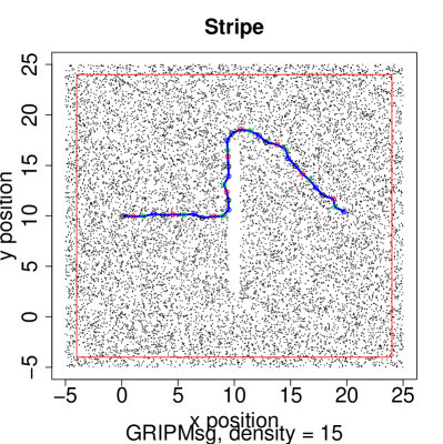
(a) Stripe.

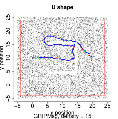
(b) U shape.

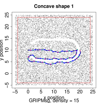
(c) Concave shape 1.

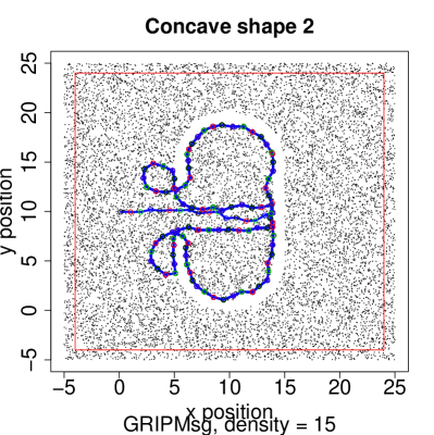
(d) Concave shape 2.

Figure 3.2: Typical behavior of GRIC (non-random version) for different obstacle shapes.

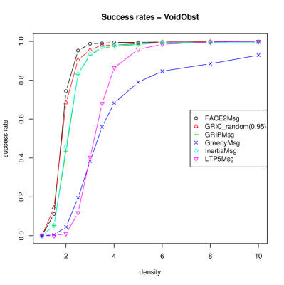
(a) Success, no obstacle.

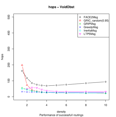
(b) Hops, no obstacle.

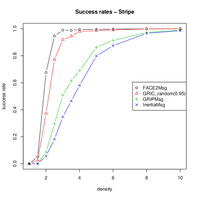
(c) Success, stripe.

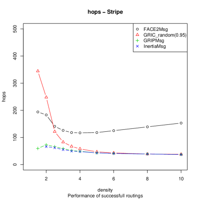
(d) Hops, stripe.

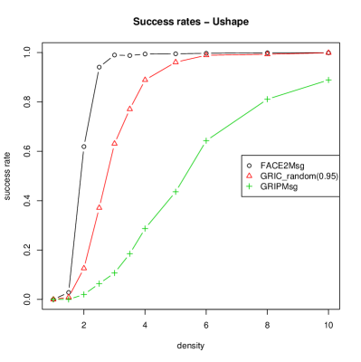
(e) Success, U shape.

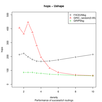
(f) Hops, U shape.

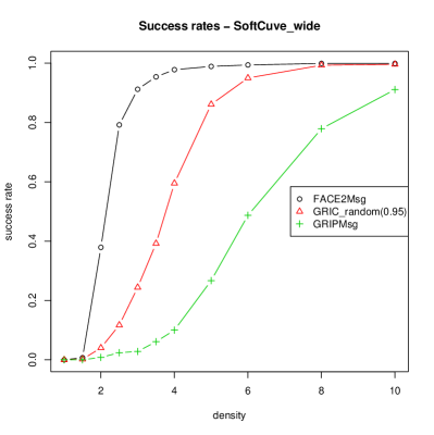
(g) Success rates, concave shape 1.

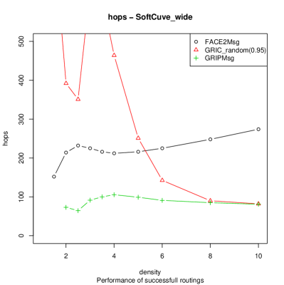
(h) Hops, concave shape 1.

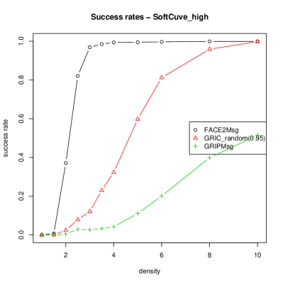
(i) Success, concave shape2.

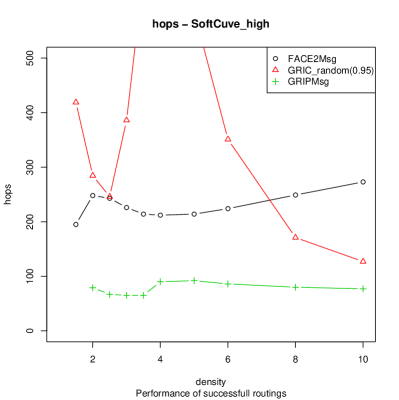
(j) Hops, concave shape2.

Figure 3.3: Success rate and hop-count when varying the network density.

3.5 Detailed analysis

3.5.1 Routing holes

Our first experimental results are in the case of no obstacles. In this case, the only difficulty is routing messages around routing holes following the local minimum problem, which is inherently dependent on network density. The results are summarised in figure 3.3(a). We can see that for medium densities ($d=5$), every protocol behaves well in terms of success rates ($100\%$ success rates, except for greedy which has only $80\%$ success rate). As well as in terms of the distance and hop-count metrics (the hop-counts are shown in figure 3.3 and the plot of travelled distances will be found in the 3.5.2 section of this appendix.). However, when the density drops, algorithms start failing: first LTP (when the density gets below $d=4$), then Inertia and $\textbf{ {GRIC}}^{-}$ when density gets below $2.5$. We observe that although success rates drop for $d\leq 2$ for $\textbf{ {GRIC}}^{+}$ , so does the success rate of FACE2, which we interpret as the fact that $\textbf{ {GRIC}}^{+}$ fails only when the network is disconnected. In terms of success rates, this means that Inertia and $\textbf{ {GRIC}}^{-}$ are quite good, but that $\textbf{ {GRIC}}^{+}$ is even better: the power of the randomness component comes into play and makes $\textbf{ {GRIC}}^{+}$ superior to the other protocols. Looking at the distance and hop-count, $\textbf{ {GRIC}}^{+}$ is almost as good as $\textbf{ {GRIC}}^{-}$ and Inertia as soon as $d=2.5$. For $d<2.5$ $\textbf{ {GRIC}}^{+}$ is not as good but this is because Inertia and GRIC fail on hard instances (i.e. they have lower success rates).

Summarizing, $\textbf{ {GRIC}}^{+}$ successfully (with success rate close to 100% if the netowrk is connected) and efficiently routes messages in localised networks, even in the case of extremely low densities.

3.5.2 Obstacles

We next consider the case of a sensor network with obstacles. We consider four different obstacle shapes: a stripe, a U shape, and two types of semi-closed concave shapes. Those shapes can be seen on figure 3.2 together with a typical path followed by a message routed by our GRIC algorithm (as can be seen, and we shall explain why, the second type of concave shape makes GRIC fail with high probability).

We start by looking at the stripe obstacle, which is a large and hard to bypass obstacle. On figure 3.3(c) we see that $\textbf{ {GRIC}}^{+}$ successfully routes messages around stripe shaped obstacles with high probability (around 95%) even for low densities ($d\simeq 3$) and almost certainly as soon as the density is medium ($d=4$). Also, figure 3.3(c) shows that the routing is efficient since the path lengths are kept small. From our intuitive understanding of the $\textbf{ {GRIC}}^{+}$ algorithm, we believe that this excellent behavior will be reproduced for any convex shaped reasonable obstacle.

We next turn to concave shapes. The large concave shapes we consider are hard obstacle instances, with shapes which can be thought of as being message traps. However, such shapes may be reasonable in real world scenarios. For example, a block of buildings could resemble the U-shaped obstacles. The first concave shape may be less realistic (it seems to be intentionally designed as a message trap), however the GRIC algorithm still behaves reasonably well (although not as well as for concave shapes). The behavior of $\textbf{ {GRIC}}^{+}$ is very similar in the case of the U shape obstacle and the first concave shape, (c.f. figure 3.3(e) and 3.4). The conclusion is that $\textbf{ {GRIC}}^{+}$ routes messages almost surely and efficiently around those two obstacles, but only if the network density if medium to high ($d$ between $5$ and $6$). In short, the finding of those experiments is that $\textbf{ {GRIC}}^{+}$ bypasses some concave shapes but only if the network density is increased. Finally, we show a concave shaped obstacle, the second concave shaped obstacle (c.f. figure 3.2), for which $\textbf{ {GRIC}}^{+}$ fails. Simulation results, summarized on figure 3.4, show that the the success rate only becomes good for very high densities ($d\simeq 8$). Furthermore, the path length is high (as can be seen on plot of figure 3.3(i) and 3.3(j)). As a conclusion, the $\textbf{ {GRIC}}^{+}$ algorithm is incapable of efficiently routing messages around the second concave shape of figure 3.2. The reason the algorithm fails is the following. We can see on the last plot of figure 3.2 what happens with $\textbf{ {GRIC}}^{-}$ and the second concave shape. $\textbf{ {GRIC}}^{-}$ successfully routes the message out of the obstacle. However, because following the contour of the obstacle would require a very sharp turn, inertia prevents the right-hand rule from making the message follow the contour of the obstacle closely. This is also true for the other obstacles. The difference here is that the influence of the message’s destination on the massage’s trajectory unfortunately makes the message fall back into the obstacle. The randomized version $\textbf{ {GRIC}}^{+}$ will eventually get the message out of the obstacle after several repeated failed attempts, but by then the message path, as seen on figure 3.3(i), will not be of competitive length anymore. Finally, we present in figures 3.3(g) and 3.3(h) the results for the concave shape 1 (c.f. figure 3.2(c)) which are comparable to those for the U shape obstacle (c.f. figure 3.2(b)).

Additional results

This section contains additional figures. Figure 3.4 gives the travelled median Euclidean distances as measured in our experiments. It turns out that those figures do not give out much more information than what is already available through observing the hop-count metric given in figure 3.3, but we include them for completeness.

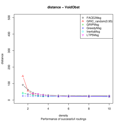
(a) No obstacle.

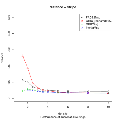
(b) Stripe.

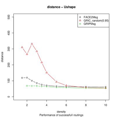
(c) U shape.

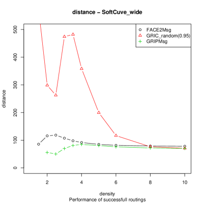
(d) Concave shape 1

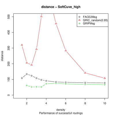
(e) Concave shape 2.

Figure 3.4: Euclidean travelled distances

Chapter 4 Conclusion

We propose the GRIC algorithm, a new geographic routing algorithm for wireless sensor networks. To our knowledge, it is the first successful implementation of the right-hand rule idea -an idea successfully used in the celebrated FACE family of algorithms- that runs on the full communication graph, i.e. that does rely on a preliminary planarization phase. Therefore, it overcomes the limitations inherent to the FACE family of algorithms while keeping its main characteristics: near 100% success rates (when no obstacles are present) and the capacity to route messages around some complex obstacles. Furthermore, routing is on demand (i.e. it is all-to-all) and requires no topology maintenance besides keeping track of the outbound links, which do not even need to be symmetric. GRIC thus surpasses all previous similar “lightweight” and simple geographic routing algorithms (which have comparatively low success rates and simply fail in the presence of large obstacles). We therefore believe that GRIC substantially improves the state of the art of geographic routing algorithms, arguably one of the most important routing paradigms for wireless sensor networks.

Bibliography

- [ACM+04] T. Antoniou, I. Chatzigiannakis, G. Mylonas, S. Nikoletseas, and A. Boukerche. A new energy efficient and fault-tolerant protocol for data propagation in smart dust networks using varying transmission range. In 37th ACM/IEEE Simulation Symposium (ANSS), pages 43–52, Hyatt Regency Crystal City, Arlington, VA, USA, April 2004. IEEE Computer Society.
- [AKJ05] Nadeem Ahmed, Salil S. Kanhere, and Sanjay Jha. The holes problem in wireless sensor networks: a survey. SIGMOBILE Mob. Comput. Commun. Rev., 9(2):4–18, 2005.
- [ASSC02] I. F. Akyildiz, W. Su, Y .Sankarasubramaniam, and E. Cayirci. Wireless sensor networks: a survey. Computer Networks, 38:393–422, March 2002.
- [Beu05] Jan Beutel. Location management in wireless sensor networks. In Handbook of Sensor Networks: Compact Wireless and Wired Systems. CRC Press, 2005.
- [BFNO03] Lali Barriere, Pierre Fraigniaud, Lata Narayanan, and Jaroslav Opatrny. Robust position-based routing in wireless ad hoc networks with irregular transmission ranges. Wireless Communications and Mobile Computing, 3:141 – 153, Mars 2003.
- [BMSU99] Prosenjit Bose, Pat Morin, Ivan Stojmenovic, and Jorge Urrutia. Routing with guaranteed delivery in ad hoc wireless networks. In DIALM ’99: Proceedings of the 3rd international workshop on Discrete algorithms and methods for mobile computing and communications, pages 48–55, New York, NY, USA, 1999. ACM Press.
- [CDNS04] I. Chatzigiannakis, T. Dimitriou, S. Nikoletseas, and P. Spirakis. A probabilistic forwarding protocol for efficient data propagation in sensor networks. In European Wireless Conference on Mobility and Wireless Systems beyond 3G (EW 2004), pages 344–350, 2004.
- [CDNS06] I. Chatzigiannakis, T. Dimitriou, S. Nikoletseas, and P. Spirakis. A probabilistic forwarding protocol for efficient data propagation in sensor networks. Journal of Ad hoc Networks, 4:621–635, 2006.
- [CKN06] Ioannis Chatzigiannakis, Athanasios Kinalis, and Sotiris Nikoletseas. Efficient and robust data dissemination using limited extra network knowledge. In 2nd IEEE International Conference on Distributed Computing in Sensor Systems (DCOSS), pages 218–233, San Francisco, USA, June 2006.
- [CMN06] Ioannis Chatzigiannakis, Georgios Mylonas, and Sotiris Nikoletseas. Modeling and evaluation of the effect of obstacles on the performance of wireless sensor networks. In 39th ACM/IEEE Simulation Symposium (ANSS), pages 50–60, Los Alamitos, CA, USA, 2006. IEEE Computer Society.
- [CNS02] Ioannis Chatzigiannakis, Sotiris Nikoletseas, and Paul Spirakis. Smart dust protocols for local detection and propagation. In POMC ’02: Proceedings of the second ACM international workshop on Principles of mobile computing, pages 9–16, New York, NY, USA, 2002. ACM Press.
- [CNS05] Ioannis Chatzigiannakis, Sotiris Nikoletseas, and Paul Spirakis. Smart dust protocols for local detection and propagation. Journal of Mobile Networks (MONET), 10:621–635, 2005.
- [DSW04] Susanta Datta, Ivan Stojmenovic, and Jie Wu. Internal node and shortcut based routing with guaranteed delivery in wireless networks. Cluster Computing, 5:169–178, November 2004.
- [EGHK99] D. Estrin, R. Govindan, J. Heidemann, and S. Kumar. Next century challenges: Scalable coordination in sensor networks. In Annual International Conference on Mobile Computing and Networking (MobiCom), pages 264–270. ACM, 1999.
- [FGG06] Qing Fang, Jie Gao, and Leonidas J. Guibas. Locating and bypassing holes in sensor networks. Mobile Networks and Applications, 11(2):187–200, April 2006.
- [Fin87] G. G. Finn. Routing and addressing problems in large metropolitan-scale internetworks. Technical Report ISI/RR-87-180, Information Sciences Institute, Mars 1987.
- [GEG+03] B. Greenstein, D. Estrin, R. Govindan, S. Ratnasamy, and S. Shenker. DIFS: A distributed index for features in sensor networks. Ad Hoc Networks, 1:333–349, September 2003.
- [HB01] Jeffrey Hightower and Gaetano Borriello. Location systems for ubiquitous computing. Computer, 34(8):57–66, 2001.
- [Hem89] A. Hemmerling. Labyrinth Problems: Labyrinth-Searching Abilities of Automata. B.G. Teubner, Leipzig, 1989.
- [HHB+03] Tian He, Chengdu Huang, Brian M. Blum, John A. Stankovic, and Tarek Abdelzaher. Range-free localization schemes for large scale sensor networks. In MobiCom ’03: Proceedings of the 9th annual international conference on Mobile computing and networking, pages 81–95, New York, NY, USA, 2003. ACM Press.
- [IGE+03] C. Intanagonwiwat, R. Govindan, D. Estrin, J. Heidemann, and F. Silva. Directed diffusion for wireless sensor networking. Transactions on Networking, 11(1):2–16, February 2003.
- [KGKS05a] Young-Jin Kim, Ramesh Govindan, Brad Karp, and Scott Shenker. Geographic routing made practical. In Proceedings of the 2nd Symposium on Networked Systems Design and Implementation (NSDI ’05), Boston, Massachusetts, USA, May 2005.
- [KGKS05b] Young-Jin Kim, Ramesh Govindan, Brad Karp, and Scott Shenker. On the pitfalls of geographic face routing. In DIALM-POMC ’05: Proceedings of the 2005 joint workshop on Foundations of mobile computing, pages 34–43, New York, NY, USA, 2005. ACM Press.
- [KGKS06] Young-Jin Kim, Ramesh Govindan, Brad Karp, and Scott Shenker. Lazy cross-link removal for geographic routing. In SenSys ’06: Proceedings of the 4th international conference on Embedded networked sensor systems, pages 112–124, New York, NY, USA, 2006. ACM Press.
- [KK00] Brad Karp and H. T. Kung. GPSR: greedy perimeter stateless routing for wireless networks. In MobiCom ’00: Proceedings of the 6th annual international conference on Mobile computing and networking, pages 243–254, New York, NY, USA, 2000. ACM Press.
- [KNS06] Johnson Kuruvila, Amiya Nayak, and Ivan Stojmenovic. Progress and location based localized power aware routing for ad hoc and sensor wireless netwroks. International Journal of Distributed Sensor Networks, 2:147–159, 2006.
- [KSU99] Evangelos Kranakis, Harvinder Singh, and Jorge Urrutia. Compass routing on geometric networks. In Proc. 11 th Canadian Conference on Computational Geometry, pages 51–54, Vancouver, August 1999.
- [KW05] Holger Karl and Andreas Willig. Protocols and Architectures for Wireless Sensor Networks. Wiley, 2005.
- [KWBP03] B. Krishnamachari, S.B. Wicker, R. Bejar, and M. Pearlman. Critical Density Thresholds in Distributed Wireless Networks, pages 279–296. Kluwer Academic Publishers, USA, 2003.
- [KWZ03] Fabian Kuhn, Roger Wattenhofer, and Aaron Zollinger. Worst-case optimal and average-case efficient geometric ad-hoc routing. In MobiHoc ’03: Proceedings of the 4th ACM international symposium on Mobile ad hoc networking & computing, pages 267–278, New York, NY, USA, 2003. ACM Press.
- [KWZZ03] Fabian Kuhn, Roger Wattenhofer, Yan Zhang, and Aaron Zollinger. Geometric ad-hoc routing: of theory and practice. In PODC ’03: Proceedings of the twenty-second annual symposium on Principles of distributed computing, pages 63–72, New York, NY, USA, 2003. ACM Press.
- [LLM06] Ben Leong, Barbara Liskov, and Robert Morris. Geogrpahic without planarization. In Proceedings of the 3rd Symposium on Network Systems Design and Implementation (NSDI ’06), May 2006.
- [LMPR06] Pierre Leone, Luminita Moraru, Olivier Powell, and Jose Rolim. Localization algorithm for wireless ad-hoc sensor networks with traffic overhead minimization by emission inhibition. In Algorithmic Aspects of Wireless Sensor Networks, volume 4240 of Lecture Notes in Computer Science. Springer Berlin/Heidelberg, January 2006.
- [PN07] Olivier Powell and Sotiris Nikolesteas. Simple and efficient geographic routing around obstacles for wireless sensor networks. In WEA 6th Workshop on Experimental Algorithms, Rome, Italy, June 2007. Springer Verlag. To appear.
- [RAdS+00] Jan M. Rabaey, M. Josie Ammer, Julio L. da Silva, Danny Patel, and Shad Roundy. Picoradio supports ad hoc ultra-low power wireless networking. Computer, 33(7):42–48, 2000.
- [RKY+02] Sylvia Ratnasamy, Brad Karp, Li Yin, Fang Yu, Deborah Estrin, Ramesh Govindan, and Scott Shenker. GHT: a geographic hash table for data-centric storage. In WSNA ’02: Proceedings of the 1st ACM international workshop on Wireless sensor networks and applications, pages 78–87, New York, NY, USA, 2002. ACM Press.
- [RRP+03] Ananth Rao, Sylvia Ratnasamy, Christos Papadimitriou, Scott Shenker, and Ion Stoica. Geographic routing without location information. In MobiCom ’03: Proceedings of the 9th annual international conference on Mobile computing and networking, pages 96–108, New York, NY, USA, 2003. ACM Press.
- [SD04] Ivan Stojmenovic and Susanta Datta. Power and cost aware localized routing with guaranteed delivery in unit graph based ad hoc networks. Wireless Communications and Mobile Computing, 4(2):175–188, 2004.
- [SHG04] Karim Seada, Ahmed Helmy, and Ramesh Govindan. On the effect of localization errors on geographic face routing in sensor networks. In IPSN ’04: Proceedings of the third international symposium on Information processing in sensor networks, pages 71–80, New York, NY, USA, 2004. ACM Press.
- [Sto02] Ivan Stojmenovic. Position-based routing in ad hoc networks. Communications Magazine, 40:128–134, July 2002.
- [WLLP01] B. Warneke, M. Last, B. Liebowitz, and K.S.J. Pister. Smart dust: communicating with a cubic-millimeter computer. Computer, 34:44–51, January 2001.
- [YHE02] Wei Ye, J. Heidemann, and D. Estrin. An energy-efficient MAC protocol for wireless sensor networks. In INFOCOM 2002. Twenty-First Annual Joint Conference of the IEEE Computer and Communications Societies, volume 3, pages 1567– 1576, 2002.
- [ZG04] Fengh Zhao and Leonidas Guibas. Wireless Sensor Networks, an Information Processing Approach. Elsevier, 2004.
- [ZHKS04] Gang Zhou, Tian He, Sudha Krishnamurthy, and John A. Stankovic. Impact of radio irregularity on wireless sensor networks. In MobiSys ’04: Proceedings of the 2nd international conference on Mobile systems, applications, and services, pages 125–138, New York, NY, USA, 2004. ACM Press.