The Octagon Abstract Domain

Abstract

This article presents a new numerical abstract domain for static analysis by abstract interpretation. It extends a former numerical abstract domain based on Difference-Bound Matrices and allows us to represent invariants of the form $(\pm x\pm y\leq c)$, where $x$ and $y$ are program variables and $c$ is a real constant.

We focus on giving an efficient representation based on Difference-Bound Matrices—${\mathcal{O}}(n^{2})$ memory cost, where $n$ is the number of variables—and graph-based algorithms for all common abstract operators—${\mathcal{O}}(n^{3})$ time cost. This includes a normal form algorithm to test equivalence of representation and a widening operator to compute least fixpoint approximations.

I Introduction

This article presents practical algorithms to represent and manipulate invariants of the form $(\pm x\pm y\leq c)$, where $x$ and $y$ are numerical variables and $c$ is a numeric constant. It extends the analysis we previously proposed in our PADO-II article [1]. Sets described by such invariants are special kind of polyhedra called octagons because they feature at most eight edges in dimension 2 (Figure 2). Using abstract interpretation, this allows discovering automatically common errors, such as division by zero, out-of-bound array access or deadlock, and more generally to prove safety properties for programs.

Our method works well for reals and rationals. Integer variables can be assumed, in the analysis, to be real in order to find approximate but safe invariants.

Example. The very simple program described in Figure 1 simulates $M$ one-dimensional random walks of $m$ steps and stores the hits in the array $tab$. Assertions in curly braces are discovered automatically by a simple static analysis using our octagonal abstract domain. Thanks to the invariants discovered, we have the guarantee that the program does not perform out-of-bound array access at lines 2 and 10. The difficult point in this example is the fact that the bounds of the array $tab$ are not known at the time of the analysis; thus, they must be treated symbolically.

1 int $tab[-m\ldots m]$; 2 for $i=-m$ to $m$ $tab[i]=0$; $\{-m\leq i\leq m\}$ 3 for $j=1$ to $M$ do 4    int $a=0$; 5    for $i=1$ to $m$ 6     $\{\;1\leq i\leq m;\;-i+1\leq a\leq i-1\;\}$ 7     if $\mbox{rand(2)}=0$ 8       then $a=a+1$; $\{\;-i+1\leq a\leq i\;\}$ 9       else $a=a-1$; $\{\;-i\leq a\leq i-1\;\}$ 10    $tab[a]=tab[a]+1$; $\{\;-m\leq a\leq m\;\}$ 11 done;

Figure 1: Simulation of a random walk. The assertions in curly brackets $\{\ldots\}$ are discovered automatically and prove that this program does not perform index out of bound error when accessing the array $tab$.

For the sake of brevity, we omit proofs of theorems in this article. The complete proof for all theorems can be found in the author’s Master thesis [2].

II Previous Work

II-A Numerical Abstract Domains.

Static analysis has developed a successful methodology, based on the abstract interpretation framework—see Cousot and Cousot’s POPL’77 paper [3]—to build analyzers that discover invariants automatically: all we need is an abstract domain, which is a practical representation of the invariants we want to study, together with a fixed set of operators and transfer functions (union, intersection, widening, assignment, guard, etc.) as described in Cousot and Cousot’s POPL’79 article [4].

There exists many numerical abstract domains. The most used are the lattice of intervals (described in Cousot and Cousot’s ISOP’76 article [5]) and the lattice of polyhedra (described in Cousot and Halbwachs’s POPL’78 article [6]). They represent, respectively, invariants of the form $(v\in[c_{1};c_{2}])$ and $(\alpha_{1}v_{1}+\cdots+\alpha_{n}v_{n}\leq c)$, where $v,v_{1},\ldots,v_{n}$ are program variables and $c,c_{1},c_{2},\alpha_{1},\ldots,\alpha_{n}$ are constants. Whereas the interval analysis is very efficient—linear memory and time cost—but not very precise, the polyhedron analysis is much more precise (Figure 2) but has a huge memory cost—in practice, it is exponential in the number of variables.

Remark that the correctness of the program in Figure 1 depends on the discovery of invariants of the form $(a\in[-m,m])$ where $m$ must not be treated as a constant, but as a variable—its value is not known at analysis time. Thus, this example is beyond the scope of interval analysis. It can be solved, of course, using polyhedron analysis.

II-B Difference-Bound Matrices.

Several satisfiability algorithms for set of constraints involving only two variables per constraint have been proposed in order to solve Constraint Logic Programming (CLP) problems. Pratt analyses, in [7], the simple case of constraints of the form $(x-y\leq c)$ and $(\pm x\leq c)$ which he called separation theory. Shostak then extends, in [8], this to a loop residue algorithm for the case $(\alpha x+\beta y\leq c)$. However, the algorithm is complete only for reals, not for integers. Recently, Harvey and Stuckey proposed, in their ACSC’97 article [9], a complete algorithm, inspired from [8], for integer constraints of the form $(\pm x\pm y\leq c)$.

Unlike CLP, when analyzing programs, we are not only interested in testing the satisfiability of constraint sets, we also need to manipulate them and apply operators that mimic the one used to define the semantics of programs (assignments, tests, control flow junctions, loops, etc.).

The model-checking community has developed a practical representation, called Difference-Bound Matrices (DBMs), for constraints of the form $(x-y\leq c)$ and ($\pm x\leq c)$, together with many operators, in order to model-check timed automata (see Yovine’s ES’98 article [10] and Larsen, Larsson, Pettersson, and Yi’s RTSS’97 article [11]). These operators are tied to model checking and do not meet the abstract interpretation needs. This problem was addressed in our PADO-II article [1] and in Shaham, Kolodner, and Sagiv’s CC2000 article [12] which propose abstract domains based on DBMs, featuring widenings and transfer functions adapted to real-live programming languages. All these works are based on the concept of shortest-path closure already present in Pratt’s article [7] as the base of the satisfiability algorithm for constraints of the form $(x-y\leq c)$. The closure also leads to a normal form that allows easy equality and inclusion testing. Good understanding of the interactions between closure and the other operators is needed to ensure the best precision possible and termination of the analysis. These interactions are described in our PADO-II article [1].

Again, proof of the correctness of the program in Figure 1 is beyond the scope of the DBM-based abstract domains presented in [1, 12] because the invariant $(-a-m\leq 0)$ we need does not match $(x-y\leq c)$.

II-C Our Contribution.

Our goal is to propose a numerical abstract domain that is between, in term of expressiveness and cost, the interval and the polyhedron domains. The set of invariants we discover can be seen as special cases of linear inequalities; but the underlying algorithmic is very different from the one used in the polyhedron domain [6], and much more efficient.

In this article, we show that DBMs can be extended to describe invariants of the form $(\pm x\pm y\leq c)$. We build a new numerical abstract domain, called the octagon abstract domain, extending the abstract domain we presented in our PADO-II article [1] and detail algorithms implementing all operators needed for abstract interpretation. Most algorithms are adapted from [1] but some are much more complex. In particular, the closure algorithm is replaced by a strong closure algorithm.

It is very important to understand that an abstract domain is only a brick in the design of a static analyzer. For the sake of simplicity, this paper presents an application of our domain on a simple forward analysis of a toy programming language. However, one could imagine to plug this domain in various analyses, such as Bourdoncle’s Syntox analyzer [13], Deutsch’s pointer analysis [14], Dor, Rodeh, and Sagiv’s string cleanness checking [15], etc.

Section III recalls the DBM representation for potential constraints $(x-y\leq c)$. Section IV explains how DBMs can be used to represent a wider range of constraints: interval constraints $(\pm x\leq c)$, and sum constraints $(\pm x\pm y\leq c)$. We then stick to this last extension, as it is the core contribution of this article, and discuss in Section V about normal form and in Section VI about operators and transfer functions. Section VII builds two lattice structures using these operators. Section VIII presents some practical results and gives some ideas for improvement.

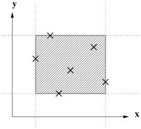
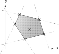
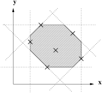
(a) (b) (c) (d)

Figure 2: A set of points (a), and its best approximation in the interval (b), polyhedron (c), and octagon (d) abstract domains.

III Difference-Bound Matrices

In this section, we recall some definitions and simple facts about Difference-Bound Matrices (DBMs) and their use in order to represent sets of invariants of the form $(x-y\leq c)$. DBMs are described in [11, 10] from a model-checking point of view and in [1] for abstract interpretation use.

Let ${\mathcal{V}}=\{v_{0},\ldots,v_{N-1}\}$ be a finite set of variables with value in a numerical set ${\mathbb{I}}$ (which can be ${\mathbb{Z}}$, ${\mathbb{Q}}$ or ${\mathbb{R}}$). We extend ${\mathbb{I}}$ to $\overline{{\mathbb{I}}}$ by adding the $+\infty$ element; the standard operations $\leq$, $=$, $+$, $\min$ and $\max$ are extended to $\overline{{\mathbb{I}}}$ as usual.

III-A Potential Constraints, DBMs.

A potential constraint over ${\mathcal{V}}$ is a constraint of the form $(v_{i}-v_{j}\leq c)$, with $v_{i},v_{j}\in{\mathcal{V}}$ and $c\in{\mathbb{I}}$. Let $C$ be a set of potential constraint over ${\mathcal{V}}$. We suppose, without loss of generality, that there do not exist two constraints $(v_{i}-v_{j}\leq c)$ and $(v_{i}-v_{j}\leq d)$ in $C$ with $c\neq d$. Then, $C$ can be represented uniquely by a $N\times N$ matrix ${{\mathbf{m}}}$ with elements in $\overline{{\mathbb{I}}}$ :

$${{\mathbf{m}}}_{ij}\;\stackrel{{\scriptstyle\triangle}}{{=}}\;\left\{\begin{array}[]{ll}c&\mbox{if $(v_{j}-v_{i}\leq c)\in C$},\\ +\infty&\mbox{elsewhere}\enspace.\end{array}\right.$$

${{\mathbf{m}}}$ is called a Difference-Bound Matrix (DBM).

III-B Potential Graph.

It is convenient to consider ${{\mathbf{m}}}$ as the adjacency matrix of a weighted graph ${\mathcal{G}}({{\mathbf{m}}})=\{{\mathcal{V}},{\mathcal{A}},w\}$, called its potential graph, and defined by:

$$\begin{array}[]{ll}\begin{array}[]{l}{\mathcal{A}}\subseteq{\mathcal{V}}\times{\mathcal{V}},\\ {\mathcal{A}}\;\stackrel{{\scriptstyle\triangle}}{{=}}\;\{(v_{i},v_{j})\;|\;{{\mathbf{m}}}_{ij}<+\infty\},\end{array}&\begin{array}[]{l}w\in{\mathcal{A}}\mapsto{\mathbb{I}},\\ w((v_{i},v_{j}))\;\stackrel{{\scriptstyle\triangle}}{{=}}\;{{\mathbf{m}}}_{ij}\enspace.\end{array}\end{array}$$

We will denote by $\langle i_{1},\ldots,i_{k}\rangle$ a finite set of nodes representing a path from node $v_{i_{1}}$ to node $v_{i_{k}}$ in ${\mathcal{G}}({{\mathbf{m}}})$. A cycle is a path such that $i_{1}=i_{k}$.

III-C $\trianglelefteqslant$ Order.

The $\leq$ order on $\overline{{\mathbb{I}}}$ induces a point-wise partial order $\trianglelefteqslant$ on the set of DBMs:

$${{\mathbf{m}}}\trianglelefteqslant{{\mathbf{n}}}\stackrel{{\scriptstyle\triangle}}{{\iff}}\forall i,j,\;{{\mathbf{m}}}_{ij}\leq{{\mathbf{n}}}_{ij}\enspace.$$

The corresponding equality relation is simply the matrix equality $=$.

III-D ${\mathcal{V}}$-domain.

Given a DBM ${{\mathbf{m}}}$, the subset of ${\mathcal{V}}\mapsto{\mathbb{I}}$ (which will be often assimilated to a subset of ${\mathbb{I}}^{N}$) verifying the constraints $\forall i,j,\;v_{j}-v_{i}\leq{{\mathbf{m}}}_{ij}$ will be denoted by ${\mathcal{D}}({{\mathbf{m}}})$ and called ${{\mathbf{m}}}$’s ${\mathcal{V}}$-domain:

$${\mathcal{D}}({{\mathbf{m}}})\;\stackrel{{\scriptstyle\triangle}}{{=}}\;\{(s_{0},\ldots,s_{N-1})\in{\mathbb{I}}^{N}\;|\;\forall i,j,\;s_{j}-s_{i}\leq{{\mathbf{m}}}_{ij}\}\enspace.$$

By extension, we will call ${\mathcal{V}}$-domain any subset of ${\mathcal{V}}\mapsto{\mathbb{I}}$ which is the ${\mathcal{V}}$-domain of some DBM.

Remark 1

We have ${{\mathbf{m}}}\trianglelefteqslant{{\mathbf{n}}}\Longrightarrow{\mathcal{D}}({{\mathbf{m}}})\subseteq{\mathcal{D}}({{\mathbf{n}}})$, but the converse is false. As a consequence, representation of ${\mathcal{V}}$-domains is not unique and we can have ${\mathcal{D}}({{\mathbf{m}}})={\mathcal{D}}({{\mathbf{n}}})$ but ${{\mathbf{m}}}\neq{{\mathbf{n}}}$ (Figure 4).

$\begin{array}[]{c|ccc}&v_{0}&v_{1}&v_{2}\\ \hline\cr v_{0}&+\infty&4&3\\ v_{1}&-1&+\infty&+\infty\\ v_{2}&-1&1&+\infty\\ \end{array}$ (a) (b) (c)

Figure 3: A DBM (a), its potential graph (b) and its ${\mathcal{V}}$-domain (c).

$\begin{array}[]{c|ccc}&v_{0}&v_{1}&v_{2}\\ \hline\cr v_{0}&+\infty&4&3\\ v_{1}&-1&+\infty&+\infty\\ v_{2}&-1&1&+\infty\\ \end{array}$ $\begin{array}[]{c|ccc}&v_{0}&v_{1}&v_{2}\\ \hline\cr v_{0}&{\bf 0}&{\bf 5}&3\\ v_{1}&-1&+\infty&+\infty\\ v_{2}&-1&1&+\infty\\ \end{array}$ (a) (b)

Figure 4: Two different DBMs with the same ${\mathcal{V}}$-domain. Remark that (a) and (b) are not even comparable with respect to $\trianglelefteqslant$.

IV Extending Difference-Bound Matrices

Discovering invariants of the single potential form $(x-y\leq c)$ is not very interesting; however DBMs can be used to represent broader constraint forms. In this section, we first present briefly how to add interval constraints $(\pm x\leq c)$. This extension is not new: [11, 1] use it instead of pure DBM. We then present our new extension allowing representation of the more general constraints $(\pm x\pm y\leq c)$.

IV-A Representing intervals.

Given a finite set of variables ${\mathcal{V}}^{0}=\{v_{0},\ldots,v_{N-1}\}$, in order to represent constraints of the form $(v_{i}-v_{j}\leq c)$ and $(\pm v_{i}\leq c)$, we simply add to ${\mathcal{V}}^{0}$ a special variable, named ${\bf 0}$, which is supposed to be always equal to 0. Constraints of the form ($v_{i}\leq c)$ and $(v_{j}\geq d)$ can then be rewritten as $(v_{i}-{\bf 0}\leq c)$ and $({\bf 0}-v_{j}\leq-d)$, which are indeed potential constraints over the set ${\mathcal{V}}=\{{\bf 0},v_{0},\ldots,v_{N-1}\}$.

We will use a $0$ superscript to denote that a DBM over ${\mathcal{V}}$ represents a set of extended constraints over ${\mathcal{V}}^{0}$. Given such a DBM ${{\mathbf{m}}}^{0}$, we will not be interested in its ${\mathcal{V}}$-domain, ${\mathcal{D}}({{\mathbf{m}}}^{0})$, which is a subset of ${\mathcal{V}}\mapsto{\mathbb{I}}$, but in its ${\mathcal{V}}^{0}$-domain, denoted by ${\mathcal{D}}^{0}({{\mathbf{m}}}^{0})$ and defined by:

$${\mathcal{D}}^{0}({{\mathbf{m}}}^{0})\;\stackrel{{\scriptstyle\triangle}}{{=}}\;\left\{\begin{array}[]{ll}(s_{0},\ldots,s_{N-1})\in\mathbb{I}^{N}\;|\\ (0,s_{0},\ldots,s_{N-1})\in{\mathcal{D}}({{\mathbf{m}}}^{0})\end{array}\right\}\subseteq{\mathcal{V}}^{0}\mapsto{\mathbb{I}}\enspace.$$

We will call ${\mathcal{V}}^{0}$-domain any subset of ${\mathcal{V}}^{0}\mapsto{\mathbb{I}}$ which is the ${\mathcal{V}}^{0}$-domain of some DBM ${{\mathbf{m}}}^{0}$. As before, ${{\mathbf{m}}}^{0}\trianglelefteqslant{{\mathbf{n}}}^{0}\Longrightarrow{\mathcal{D}}^{0}({{\mathbf{m}}}^{0})\subseteq{\mathcal{D}}^{0}({{\mathbf{n}}}^{0})$, but the converse is false.

IV-B Representing sums.

We suppose that ${\mathcal{V}}^{+}=\{v_{0},\ldots,v_{N-1}\}$ is a finite set of variables. The goal of this article is to present a new DBM extension adapted to represent constraints of the form $(\pm v_{i}\pm v_{j}\leq c)$, with $v_{i},v_{j}\in{\mathcal{V}}^{+}$ and $c\in{\mathbb{I}}$.

In order to do this, we consider that each variable $v_{i}$ in ${\mathcal{V}}^{+}$ comes in two flavors: a positive form $v^{+}_{i}$ and a negative form $v^{-}_{i}$. We introduce the set ${\mathcal{V}}=\{\;v^{+}_{0},\;v^{-}_{0},\;\ldots,\;v^{+}_{N-1},\;v^{-}_{N-1}\;\}$ and consider DBMs over ${\mathcal{V}}$. Within a potential constraint, a positive variable $v^{+}_{i}$ will be interpreted as $+v_{i}$, and a negative variable $v^{-}_{i}$ as $-v_{i}$; thus it is possible to represent $(v_{i}+v_{j}\leq c)$ by $(v^{+}_{i}-v^{-}_{j}\leq c)$. More generally, any set of constraints of the form $(\pm v_{i}\pm v_{j}\leq c)$, with $v_{i},v_{j}\in{\mathcal{V}}^{+}$ can be represented by a DBM over ${\mathcal{V}}$, following the translation described in Figure 5.

Remark 2

We do not need to add a special variable ${\bf 0}$ to represent interval constraints as we did before. Constraints of the form $(v_{i}\leq c)$ and $(v_{i}\geq c)$ can be represented as $(v^{+}_{i}-v^{-}_{i}\leq 2c)$ and $(v^{-}_{i}-v^{+}_{i}\leq-2c)$.

$\begin{array}[]{|cc|cc|}\hline\cr\vrule\lx@intercol\hfil\mbox{constraint over ${\mathcal{V}}^{+}$}\hfil\lx@intercol\vrule\lx@intercol&\lx@intercol\hfil\mbox{constraint(s) over ${\mathcal{V}}$}\hfil\lx@intercol\vrule\lx@intercol\\ \hline\cr v_{i}-v_{j}\leq c&(i\neq j)&v_{i}^{+}-v_{j}^{+}\leq c,&v_{j}^{-}-v_{i}^{-}\leq c\\ v_{i}+v_{j}\leq c&(i\neq j)&v_{i}^{+}-v_{j}^{-}\leq c,&v_{j}^{+}-v_{i}^{-}\leq c\\ -v_{i}-v_{j}\leq c&(i\neq j)&v_{j}^{-}-v_{i}^{+}\leq c,&v_{i}^{-}-v_{j}^{+}\leq c\\ v_{i}\leq c&&\lx@intercol\hfil v_{i}^{+}-v_{i}^{-}\leq 2c\hfil\lx@intercol\vrule\lx@intercol\\ v_{i}\geq c&&\lx@intercol\hfil v_{i}^{-}-v_{i}^{+}\leq-2\hfil\lx@intercol\vrule\lx@intercol\\ \hline\cr\end{array}$

Figure 5: Translation between extended constraints over ${\mathcal{V}}^{+}$ and potential constraints over ${\mathcal{V}}$.

IV-C Index Notation.

We will use a $+$ superscript to denote that a DBM over ${\mathcal{V}}$ represents a set of extended constraints over ${\mathcal{V}}^{+}$. Such a DBM ${{\mathbf{m}}}^{+}$ is a $2N\times 2N$ matrix with the following convention: a row or column index of the form $2i,\;i<N$ corresponds to the variable $v^{+}_{i}$ and an index of the form $2i+1,\;i<N$ corresponds to the variable $v^{-}_{i}$.

We introduce the $\cdot\mapsto{\overline{\cdot}}$ operator on indices defined by ${\,\bar{\imath}}\;\stackrel{{\scriptstyle\triangle}}{{=}}\;i\oplus 1$—where $\oplus$ is the bit-wise exclusive or operator—so that, if $i$ corresponds to $v^{+}_{j}$, then ${\,\bar{\imath}}$ corresponds to $v^{-}_{j}$ and if $i$ corresponds to $v^{-}_{j}$, then ${\,\bar{\imath}}$ corresponds to $v^{+}_{j}$.

IV-D Coherence.

Figure 5 shows that some constraints over ${\mathcal{V}}^{+}$ can be represented by different potential constraints over ${\mathcal{V}}$. A DBM ${{\mathbf{m}}}^{+}$ will be said to be coherent if two potential constraints over ${\mathcal{V}}$ corresponding to the same constraint over ${\mathcal{V}}^{+}$ are either both represented in ${{\mathbf{m}}}^{+}$, or both absent. Thanks to the $\cdot\mapsto{\overline{\cdot}}$ operator we introduced, coherence can be easily characterized:

Theorem 1

${{\mathbf{m}}}^{+}\mbox{ is coherent }\iff\forall i,j,\;{{\mathbf{m}}}^{+}_{ij}={{\mathbf{m}}}^{+}_{{\bar{\jmath}}{\,\bar{\imath}}}\enspace.$

$\Box$

In the following, DBMs with a $+$ superscript will be assumed to be coherent.

IV-E ${\mathcal{V}}^{+}$-domain.

As for the simple interval extension, the ${\mathcal{V}}$-domain of a DBM ${{\mathbf{m}}}^{+}$ is not of interest: we need to get back in ${\mathcal{V}}^{+}\mapsto{\mathbb{I}}$ and take into account the fact that variables in ${\mathcal{V}}$ are not independent but related by $v^{+}_{i}=-v^{-}_{i}$. Thus, we define the ${\mathcal{V}}^{+}$-domain of ${{\mathbf{m}}}^{+}$ and denote by ${\mathcal{D}}^{+}({{\mathbf{m}}}^{+})$ the set:

$${\mathcal{D}}^{+}({{\mathbf{m}}}^{+})\;\stackrel{{\scriptstyle\triangle}}{{=}}\;\left\{\begin{array}[]{ll}(s_{0},\ldots,s_{N-1})\in{\mathbb{I}}^{N}\;|\\ (s_{0},-s_{0},\ldots,s_{N-1},-s_{N-1})\in{\mathcal{D}}({{\mathbf{m}}}^{+})\end{array}\right\}.$$

We will call octagon any subset of ${\mathcal{V}}^{+}\mapsto{\mathbb{I}}$ which is the ${\mathcal{V}}^{+}$-domain of some coherent DBM ${{\mathbf{m}}}^{+}$. As before, ${{\mathbf{m}}}^{+}\trianglelefteqslant{{\mathbf{n}}}^{+}\Longrightarrow{\mathcal{D}}^{+}({{\mathbf{m}}}^{+})\subseteq{\mathcal{D}}^{+}({{\mathbf{n}}}^{+})$, but the converse is false.

V Emptiness Test and Normal Forms

We saw in Figure 4 that two different DBMs can have the same ${\mathcal{V}}$-domain. Fortunately, there exists a normal form for DBMs representing non-empty octagons.

In this section, we first recall the normal form for classical DBMs ${{\mathbf{m}}}$, and then show how it can be adapted to DBMs ${{\mathbf{m}}}^{+}$ representing non-empty octagons. Unfortunately, our adaptation does not work very well with integers.

The potential graph interpretation of DBMs will be very helpful to understand the algorithms presented.

V-A Emptiness Test.

The following graph-oriented theorem allows us to perform emptiness testing for ${\mathcal{V}}$-domains, ${\mathcal{V}}^{0}$-domains and octagons:

Theorem 2

1. ${\mathcal{D}}({{\mathbf{m}}})=\emptyset\iff{\mathcal{G}}({{\mathbf{m}}})$ has a cycle with a strictly negative weight.

2. ${\mathcal{D}}({{\mathbf{m}}}^{0})=\emptyset\iff{\mathcal{D}}^{0}({{\mathbf{m}}}^{0})=\emptyset$.

3. If ${\mathbb{I}}\neq{\mathbb{Z}}$, then ${\mathcal{D}}({{\mathbf{m}}}^{+})=\emptyset\iff{\mathcal{D}}^{+}({{\mathbf{m}}}^{+})=\emptyset$.

   If ${\mathbb{I}}={\mathbb{Z}}$, then ${\mathcal{D}}({{\mathbf{m}}}^{+})=\emptyset\Longrightarrow{\mathcal{D}}^{+}({{\mathbf{m}}}^{+})=\emptyset$, but the converse is false (Figure 6).

$\Box$

If ${\mathbb{I}}\neq{\mathbb{Z}}$, in order to check whether the ${\mathcal{V}}^{+}$-domain of a DBM ${{\mathbf{m}}}^{+}$ is empty, we simply have to check for cycles with a strictly negative weight in ${\mathcal{G}}({{\mathbf{m}}}^{+})$ using, for example, the well-known Bellman-Ford algorithm which runs in ${\mathcal{O}}(N^{3})$ time and is described in Cormen, Leiserson and Rivest’s classical algorithmic textbook [16, §25.3].

Figure 6 gives an example where our algorithm fails when dealing with integers. Indeed, we have ${\mathcal{D}}({{\mathbf{m}}}^{+})=\{(3+x,3-x,3+y,3-y)\;|\;\forall x,y\in{\mathbb{Z}}\}$ which is not empty, but all these solutions over $\{v_{0}^{+},v_{0}^{-},v_{1}^{+},v_{1}^{-}\}$ correspond to the singleton $\{(3/2,3/2)\}$ when we get back to $\{v_{0},v_{1}\}$, which is not an acceptable solution in ${\mathbb{Z}}^{2}$, so ${\mathcal{D}}^{+}({{\mathbf{m}}}^{+})$ should be empty. The problem is that a DBM ${{\mathbf{m}}}^{+}$ with coefficients in ${\mathbb{Z}}$ can represent constraints that use not only integers, but also half-integers constants—such as $v_{1}\geq 3/2$ in Figure 6.

\begin{picture}(0.0,0.0)\end{picture} (a) (b)

Figure 6: A potential graph ${\mathcal{G}}({{\mathbf{m}}}^{+})$ in ${\mathbb{Z}}$ with no strictly negative cycle (a) and the corresponding ${\mathcal{V}}^{+}$-domain (b) ${\mathcal{D}}^{+}({{\mathbf{m}}}^{+})=\{(\frac{3}{2},\frac{3}{2})\}$ which is empty in ${\mathbb{Z}}^{2}$.

V-B Closure.

Given a DBM ${{\mathbf{m}}}$, the ${\mathcal{V}}$-domain of which is not empty, ${\mathcal{G}}({{\mathbf{m}}})$ has no strictly negative cycle, so its shortest-path closure—or simply closure—${{\mathbf{m}}}^{*}$ is well-defined by:

$$\left\{\begin{array}[]{ll}{{\mathbf{m}}}^{*}_{ii}\;\stackrel{{\scriptstyle\triangle}}{{=}}\;0,&\\ \displaystyle{{\mathbf{m}}}^{*}_{ij}\;\stackrel{{\scriptstyle\triangle}}{{=}}\;\min_{\begin{subarray}{c}1\leq M\\ \langle i=i_{1},i_{2},\ldots,i_{M}=j\rangle\quad\end{subarray}}\sum_{k=1}^{M-1}{{\mathbf{m}}}_{i_{k}i_{k+1}}&\mbox{ if }i\neq j\enspace.\end{array}\right.$$

The idea of closure relies on the fact that, if $\langle i=i_{1},i_{2},\ldots,i_{M}=j\rangle$ is a path from $v_{i}$ to $v_{j}$, then the constraint $v_{j}-v_{i}\leq\sum_{k=1}^{M-1}{{\mathbf{m}}}_{i_{k}i_{k+1}}$ can be derived from ${{\mathbf{m}}}$ by adding the potential constraints $v_{i_{k+1}}-v_{i_{k}}\leq{{\mathbf{m}}}_{i_{k}i_{k+1}},\;1\leq k\leq M-1$. This is an implicit potential constraint as it does not appear directly in ${{\mathbf{m}}}$. In the closure, we replace each potential constraint $v_{j}-v_{i}\leq{{\mathbf{m}}}_{ij}$ by the tightest implicit constraint we can find by summation over paths of ${\mathcal{G}}({{\mathbf{m}}})$ if $i\neq j$, or by $0$ if $i=j$ ($0$ is indeed the smallest value taken by $v_{i}-v_{i}$).

We have the following theorem:

Theorem 3

1. ${{\mathbf{m}}}={{\mathbf{m}}}^{*}\iff\forall i,j,k,\;{{\mathbf{m}}}_{ij}\leq{{\mathbf{m}}}_{ik}+{{\mathbf{m}}}_{kj}$ and $\forall i,\;{{\mathbf{m}}}_{ii}=0$ (Local Definition).

2. $\forall i,j,\;$ if ${{\mathbf{m}}}^{*}_{ij}\neq+\infty$, then $\exists(s_{0},\ldots,s_{N-1})\in{\mathcal{D}}({{\mathbf{m}}})$ such that $s_{j}-s_{i}={{\mathbf{m}}}^{*}_{ij}$ (Saturation).

3. ${{\mathbf{m}}}^{*}=\inf_{\trianglelefteqslant}\{{{\mathbf{n}}}\;|\;{\mathcal{D}}({{\mathbf{n}}})={\mathcal{D}}({{\mathbf{m}}})\}$ (Normal Form).

$\Box$

Theorem 3.2 proves that the closure is indeed a normal form. Theorem 3.1 leads to a closure algorithm inspired by the Floyd-Warshall shortest-path algorithm. This algorithm is described in Figure 7 and runs in ${\mathcal{O}}(N^{3})$ time. Theorem 3.2 is crucial to analyze precision of some operators (such as projection and union).

Remark 3

The closure is also a normal form for DBMs representing non-empty ${\mathcal{V}}^{0}$-domains:
$({{\mathbf{m}}}^{0})^{*}=\inf_{\trianglelefteqslant}\{{{\mathbf{n}}}^{0}\;|\;{\mathcal{D}}^{0}({{\mathbf{n}}}^{0})={\mathcal{D}}^{0}({{\mathbf{m}}}^{0})\}$.

 $\begin{array}[]{c}\left\{\begin{array}[]{lcl}{{\mathbf{m}}}_{0}&\;\stackrel{{\scriptstyle\triangle}}{{=}}&{{\mathbf{m}}},\\ {{\mathbf{m}}}_{k+1}&\;\stackrel{{\scriptstyle\triangle}}{{=}}&C_{k}({{\mathbf{m}}}_{k})\quad\forall k,\;0\leq k<N,\\ {{\mathbf{m}}}^{*}&\;\stackrel{{\scriptstyle\triangle}}{{=}}&{{\mathbf{m}}}_{N},\end{array}\right.\\ \\ \mbox{where $C_{k}$ is defined, $\forall k$, by:}\\ \\ \left\{\begin{array}[]{l}\left[C_{k}({{\mathbf{n}}})\right]_{ii}\;\stackrel{{\scriptstyle\triangle}}{{=}}\;0,\\ \left[C_{k}({{\mathbf{n}}})\right]_{ij}\;\stackrel{{\scriptstyle\triangle}}{{=}}\;\min({{\mathbf{n}}}_{ij},{{\mathbf{n}}}_{ik}+{{\mathbf{n}}}_{kj})\quad\forall i\neq j\enspace.\end{array}\right.\end{array}$  

Figure 7: Closure algorithm derived from the Floyd-Warshall shortest-path algorithm.

V-C Strong Closure.

We now focus on finding a normal form for DBMs representing non-empty octagons. The solution presented above does not work because two different DBMs can have the same ${\mathcal{V}}^{+}$-domain but different ${\mathcal{V}}$-domains, and so the closure $({{\mathbf{m}}}^{+})^{*}$ of ${{\mathbf{m}}}^{+}$ is not the smallest DBM—with respect to the $\trianglelefteqslant$ order—that represents the octagon ${\mathcal{D}}^{+}({{\mathbf{m}}}^{+})$. The problem is that the set of implicit constraints gathered by summation of constraints over paths of ${\mathcal{G}}({{\mathbf{m}}}^{+})$ is not sufficient. Indeed, we would like to deduce $(v_{i}^{+}-v_{j}^{-}\leq(c+d)/2)$ from $(v_{i}^{+}-v_{i}^{-}\leq c)$ and $(v_{j}^{+}-v_{j}^{-}\leq d$), which is not possible because the set of edges $\{(v_{i}^{-},v_{i}^{+}),(v_{j}^{-},v_{j}^{+})\}$ does not form a path (Figure 9).

Here is a more formal description of a normal form, called the strong closure, adapted from the closure:

Definition 1

${{\mathbf{m}}}^{+}$ is strongly closed if and only if

• ${{\mathbf{m}}}^{+}$ is coherent: $\forall i,j,\;{{\mathbf{m}}}^{+}_{ij}={{\mathbf{m}}}^{+}_{{\bar{\jmath}}{\,\bar{\imath}}}$;

• ${{\mathbf{m}}}^{+}$ is closed: $\forall i,\;{{\mathbf{m}}}^{+}_{ii}=0$ and $\forall i,j,k,\;{{\mathbf{m}}}^{+}_{ij}\leq{{\mathbf{m}}}^{+}_{ik}+{{\mathbf{m}}}^{+}_{kj}$;

• $\forall i,j,\;$ ${{\mathbf{m}}}^{+}_{ij}\leq({{\mathbf{m}}}^{+}_{i{\,\bar{\imath}}}+{{\mathbf{m}}}^{+}_{{\bar{\jmath}}j})/2$.

$\Box$

From this definition, we derive the strong closure algorithm ${{\mathbf{m}}}^{+}\mapsto({{\mathbf{m}}}^{+})^{\bullet}$ described in Figure 8. The algorithm looks a bit like the closure algorithm of Figure 7 and also runs in ${\mathcal{O}}(N^{3})$ time. It uses two auxiliary functions $C^{+}_{k}$ and $S^{+}$. The $C^{+}_{k}$ function looks like the $C_{k}$ function used in the closure algorithm except it is designed to maintain coherence; each $C^{+}_{k}$ application is a step toward closure. The $S^{+}$ function ensures that $\forall i,j,\;\left[S^{+}({{\mathbf{m}}}^{+})\right]_{ij}\leq(\left[S^{+}({{\mathbf{m}}}^{+})\right]_{i{\,\bar{\imath}}}+\left[S^{+}({{\mathbf{m}}}^{+})\right]_{{\bar{\jmath}}j})/2$ while maintaining coherence.

There is no simple explanation for the complexity of $C^{+}_{k}$; the five terms in the min statement appear naturally when trying to prove that, when interleaving $C^{+}_{k}$ and $S^{+}$ steps, what was gained before will not be destroyed in the next step.

The following theorem holds for ${\mathbb{I}}\neq{\mathbb{Z}}$:

Theorem 4

1. ${{\mathbf{m}}}^{+}=({{\mathbf{m}}}^{+})^{\bullet}\iff{{\mathbf{m}}}^{+}\mbox{ is strongly closed}$.

2. $\forall i,j,\;$ if $({{\mathbf{m}}}^{+})^{\bullet}_{ij}\neq+\infty$, then $\exists(s_{0},\ldots,s_{2N-1})\in{\mathcal{D}}({{\mathbf{m}}}^{+})$ such that $\forall k,\;s_{2k}=-s_{2k+1}$ and $s_{j}-s_{i}=({{\mathbf{m}}}^{+})^{\bullet}_{ij}$ (Saturation).

3. $({{\mathbf{m}}}^{+})^{\bullet}=\inf_{\trianglelefteqslant}\{{{\mathbf{n}}}^{+}\;|\;{\mathcal{D}}^{+}({{\mathbf{n}}}^{+})={\mathcal{D}}^{+}({{\mathbf{m}}}^{+})\}$ (Normal Form).

$\Box$

This theorem is very similar to Theorem 3. It states that, when ${\mathbb{I}}\neq{\mathbb{Z}}$, the strong closure algorithm gives a strongly closed DBM (Theorem 4.1) which is indeed a normal form (Theorem 4.3). The nice saturation property of Theorem 4.2 is useful to analyze the projection and union operators.

$\begin{array}[]{c}\left\{\begin{array}[]{lcl}{{\mathbf{m}}}^{+}_{0}&\;\stackrel{{\scriptstyle\triangle}}{{=}}&{{\mathbf{m}}}^{+},\\ {{\mathbf{m}}}^{+}_{k+1}&\;\stackrel{{\scriptstyle\triangle}}{{=}}&S^{+}(C^{+}_{2k}({{\mathbf{m}}}^{+}_{k}))\quad\forall k,\;0\leq k<N,\\ ({{\mathbf{m}}}^{+})^{\bullet}&\;\stackrel{{\scriptstyle\triangle}}{{=}}&{{\mathbf{m}}}^{+}_{N},\\ \end{array}\right.\\ \\ \mbox{where $C^{+}_{k}$ is defined, $\forall k$, by:}\\ \\ \left\{\begin{array}[]{ll}\left[C^{+}_{k}({{\mathbf{n}}}^{+})\right]_{ii}\;\stackrel{{\scriptstyle\triangle}}{{=}}\;0,\\ \left[C^{+}_{k}({{\mathbf{n}}}^{+})\right]_{ij}\;\stackrel{{\scriptstyle\triangle}}{{=}}\;\min(&{{\mathbf{n}}}^{+}_{ij},\;({{\mathbf{n}}}^{+}_{ik}+{{\mathbf{n}}}^{+}_{kj}),\\ &({{\mathbf{n}}}^{+}_{i{\bar{k}}}+{{\mathbf{n}}}^{+}_{{\bar{k}}j}),\\ &({{\mathbf{n}}}^{+}_{ik}+{{\mathbf{n}}}^{+}_{k{\bar{k}}}+{{\mathbf{n}}}^{+}_{{\bar{k}}j}),\\ &({{\mathbf{n}}}^{+}_{i{\bar{k}}}+{{\mathbf{n}}}^{+}_{{\bar{k}}k}+{{\mathbf{n}}}^{+}_{kj})\;)\end{array}\right.\\ \\ \mbox{and $S^{+}$ is defined by:}\\ \\ \begin{array}[]{l}\left[S^{+}({{\mathbf{n}}}^{+})\right]_{ij}\;\stackrel{{\scriptstyle\triangle}}{{=}}\;\min(\;{{\mathbf{n}}}^{+}_{ij},\;({{\mathbf{n}}}^{+}_{i{\,\bar{\imath}}}+{{\mathbf{n}}}^{+}_{{\bar{\jmath}}j})/2\;)\enspace.\end{array}\end{array}$

Figure 8: Strong Closure algorithm.

  $\Longrightarrow$ (a) (b)

Figure 9: A DBM (a) and its strong closure (b). Note that (a) is closed, and that (a) and (b) have the same ${\mathcal{V}}^{+}$-domain but not the same ${\mathcal{V}}$-domain. In (b), we deduced $(v_{0}+v_{1}\leq 3)$ from $(2v_{0}\leq 2)$ and $(2v_{1}\leq 4)$, so it is smaller than (a) with respect to $\trianglelefteqslant$.

V-D Discussions about ${\mathbb{Z}}$.

Classical DBMs and the interval constraint extension work equally well on reals, rationals and integers. However, our extension does not handle integers properly.

When ${\mathbb{I}}={\mathbb{Z}}$, the strong closure algorithm does not lead to the smallest DBM with the same ${\mathcal{V}}^{+}$-domain. For example, knowing that $x$ is an integer, the constraint $2x\leq 2c$ should be deduced from $2x\leq 2c+1$, which the strong closure algorithm fails to do. More formally, Definition 1 is not sufficient; our normal form should also respect: $\forall i,\;{{\mathbf{m}}}^{+}_{i{\,\bar{\imath}}}\mbox{ is even}$. One can imagine to simply add to the strong closure algorithm a rounding phase $R^{+}$ defined by $\left[R^{+}({{\mathbf{m}}}^{+})\right]_{i{\,\bar{\imath}}}=2\lfloor{{\mathbf{m}}}^{+}_{i{\,\bar{\imath}}}/2\rfloor$ and $\left[R^{+}({{\mathbf{m}}}^{+})\right]_{ij}={{\mathbf{m}}}^{+}_{ij}$ if $i\neq{\bar{\jmath}}$, but it is tricky to make $R^{+}$ and $C^{+}_{k}$ interact correctly so we obtain a DBM which is both closed and rounded. We were unable, at the time of writing, to design such an algorithm and keep a ${\mathcal{O}}(N^{3})$ time cost.

This problem was addressed by Harvey and Stuckey in their ACSC’97 article [9]. They propose a satisfiability algorithm mixing closure and tightening steps that can be used to test emptiness and build the normal form $({{\mathbf{m}}}^{+})^{\bullet}=\inf_{\trianglelefteqslant}\{{{\mathbf{n}}}^{+}\;|\;{\mathcal{D}}^{+}({{\mathbf{n}}}^{+})={\mathcal{D}}^{+}({{\mathbf{m}}}^{+})\}$ we need. Unfortunately, this algorithm has a ${\mathcal{O}}(N^{4})$ time cost in the worst case. This algorithm has the advantage of being incremental—${\mathcal{O}}(N^{2})$ time cost per constraint changed in the DBM—which is useful for CLP problems but does not seem interesting in static analysis because many operators are point-wise and change all $(2N)^{2}$ constraints in a DBM at once.

In practice, we suggest to analyze integer variables in ${\mathbb{Q}}$ or ${\mathbb{R}}$, as it is commonly done for polyhedron analysis [6]. This method will add noise solutions, which is safe in the abstract interpretation framework because we are only interested in an upper approximation of program behaviors.

VI Operators and Transfer Functions

In this section, we describe how to implement the abstract operators and transfer functions needed for static analysis.

These are the generic ones described in [5] for the interval domain, and in [6] for the polyhedron domain: assignments, tests, control flow junctions and loops. See Section VIII for an insight on how to use theses operators to actually build an analyzer. If our abstract numerical domain is used in a more complex analysis or in a parameterized abstract domain (backward and interprocedural analysis, such as in Bourdoncle’s Syntox analyzer, Deutsch’s pointer analysis [14], etc.), one may need to add some more operators.

All the operators and transfer functions presented in this section obviously respect coherence and are adapted from our PADO-II article [1].

VI-A Equality and Inclusion Testing.

We distinguish two cases. If one or both ${\mathcal{V}}^{+}$-domains are empty, then the test is obvious. If none are empty, we use the following theorem which relies on the properties of the strong closure:

Theorem 5

1. ${\mathcal{D}}^{+}({{\mathbf{m}}}^{+})\subseteq{\mathcal{D}}^{+}({{\mathbf{n}}}^{+})\iff({{\mathbf{m}}}^{+})^{\bullet}\trianglelefteqslant{{\mathbf{n}}}^{+}$;

2. ${\mathcal{D}}^{+}({{\mathbf{m}}}^{+})={\mathcal{D}}^{+}({{\mathbf{n}}}^{+})\iff({{\mathbf{m}}}^{+})^{\bullet}=({{\mathbf{n}}}^{+})^{\bullet}$.

$\Box$

VI-B Projection.

Thanks to the saturation property of the strong closure, we can easily extract from a DBM ${{\mathbf{m}}}^{+}$ representing a non-empty octagon, the interval in which a variable $v_{i}$ ranges :

Theorem 6

$\begin{array}[]{l}\{\;t\;|\;\exists(s_{0},\ldots,s_{N-1})\in{\mathcal{D}}^{+}({{\mathbf{m}}}^{+})\mbox{ such that }s_{i}=t\;\}\\ \quad=[\;-({{\mathbf{m}}}^{+})^{\bullet}_{2i\;2i+1}/2,\;({{\mathbf{m}}}^{+})^{\bullet}_{2i+1\;2i}/2\;]\end{array}$

(interval bounds are included only if finite).

$\Box$

VI-C Union and Intersection.

The max and min operators on $\overline{{\mathbb{I}}}$ lead to point-wise least upper bound $\vee$ and greatest lower bound $\wedge$ (with respect to the $\trianglelefteqslant$ order) operators on DBMs:

$$\begin{array}[]{l}\left[{{\mathbf{m}}}^{+}\wedge{{\mathbf{n}}}^{+}\right]_{ij}\;\stackrel{{\scriptstyle\triangle}}{{=}}\;\min({{\mathbf{m}}}^{+}_{ij},{{\mathbf{n}}}^{+}_{ij});\\ \left[{{\mathbf{m}}}^{+}\vee{{\mathbf{n}}}^{+}\right]_{ij}\;\stackrel{{\scriptstyle\triangle}}{{=}}\;\max({{\mathbf{m}}}^{+}_{ij},{{\mathbf{n}}}^{+}_{ij})\enspace.\end{array}$$

These operators are useful to compute intersections and unions of octagons:

Theorem 7

1. ${\mathcal{D}}^{+}({{\mathbf{m}}}^{+}\wedge{{\mathbf{n}}}^{+})={\mathcal{D}}^{+}({{\mathbf{m}}}^{+})\cap{\mathcal{D}}^{+}({{\mathbf{n}}}^{+})$.

2. ${\mathcal{D}}^{+}({{\mathbf{m}}}^{+}\vee{{\mathbf{n}}}^{+})\supseteq{\mathcal{D}}^{+}({{\mathbf{m}}}^{+})\cup{\mathcal{D}}^{+}({{\mathbf{n}}}^{+})$.

3. If ${{\mathbf{m}}}^{+}$ and ${{\mathbf{n}}}^{+}$ represent non-empty octagons, then:

   $\begin{array}[]{l}(({{\mathbf{m}}}^{+})^{\bullet})\vee(({{\mathbf{n}}}^{+})^{\bullet})=\\ \quad\inf_{\trianglelefteqslant}\{{{\mathbf{o}}}^{+}\;|\;{\mathcal{D}}^{+}({{\mathbf{o}}}^{+})\supseteq{\mathcal{D}}^{+}({{\mathbf{m}}}^{+})\cup{\mathcal{D}}^{+}({{\mathbf{n}}}^{+})\}.\end{array}$

$\Box$

Remark that the intersection is always exact, but the union of two octagons is not always an octagon, so we compute an upper approximation. In order to get the best—smallest—approximation for the union, we need to use the strong closure algorithm, as stated in Theorem 7.3.

Another consequence of Theorem 7.3 is that if the two arguments of $\vee$ are strongly closed, then the result is also strongly closed. Dually, the arguments of $\wedge$ do not need to be strongly closed in order to get the best precision, but the result is seldom strongly closed—even if the arguments are. This situation is similar to what is described in our PADO-II article [1]. Shaham, Kolodner, and Sagiv fail to analyze this result in their CC2000 article [12] and perform a useless closure after the union operator.

VI-D Widening.

Program semantics often use fixpoints to model arbitrary long computations such as loops. Fixpoints are not computable in the octagon domain—as it is often the case for abstract domains—because it is of infinite height. Thus, we define a widening operator, as introduced in P.Cousot’s thesis [17, §4.1.2.0.4], to compute iteratively an upper approximation of the least fixpoint $\bigvee_{i\in\mathbb{N}}F^{i}({{\mathbf{m}}}^{+})$ greater than ${{\mathbf{m}}}^{+}$ of an operator $F$:

$$\left[{{\mathbf{m}}}^{+}\triangledown{{\mathbf{n}}}^{+}\right]_{ij}\;\stackrel{{\scriptstyle\triangle}}{{=}}\;\left\{\begin{array}[]{ll}{{\mathbf{m}}}^{+}_{ij}&\mbox{ if }{{\mathbf{n}}}^{+}_{ij}\leq{{\mathbf{m}}}^{+}_{ij},\\ +\infty&\mbox{elsewhere}\enspace.\end{array}\right.$$

The idea behind this widening is to remove in ${{\mathbf{m}}}^{+}$ the constraints that are not stable by union with ${{\mathbf{n}}}^{+}$; thus it is very similar to the standard widenings used on the domains of intervals [5] and polyhedra [6]. [12] proposes a similar widening on the set of DBMs representing ${\mathcal{V}}$-domains.

The following theorem proves that $\triangledown$ is a widening in the octagon domain:

Theorem 8

1. ${\mathcal{D}}^{+}({{\mathbf{m}}}^{+}\triangledown{{\mathbf{n}}}^{+})\supseteq{\mathcal{D}}^{+}({{\mathbf{m}}}^{+})\cup{\mathcal{D}}^{+}({{\mathbf{n}}}^{+})$.

2. For all chains $({{\mathbf{n}}}^{+}_{i})_{i\in\mathbb{N}}$, the chain defined by induction:

   $${{\mathbf{m}}}^{+}_{i}\;\stackrel{{\scriptstyle\triangle}}{{=}}\;\left\{\begin{array}[]{ll}({{\mathbf{n}}}^{+}_{0})^{\bullet}&\mbox{ if }i=0,\\ {{\mathbf{m}}}^{+}_{i-1}\triangledown(({{\mathbf{n}}}^{+}_{i})^{\bullet})&\mbox{ elsewhere},\\ \end{array}\right.$$

   is increasing, ultimately stationary, and with a limit greater than $\bigvee_{i\in\mathbb{N}}({{\mathbf{n}}}^{+}_{i})^{\bullet}$.

$\Box$

As for the union operator, the precision of the $\triangledown$ operator is improved if its right argument is strongly closed; this is why we ensure the strong closure of ${{\mathbf{n}}}^{+}_{i}$ when computing ${{\mathbf{m}}}^{+}_{i}$ in Theorem 8.2.

One can be tempted to force the strong closure of the left argument of the widening by replacing the induction step in Theorem 8.2 by: ${{\mathbf{m}}}^{+}_{i}=({{\mathbf{m}}}^{+}_{i-1}\triangledown(({{\mathbf{n}}}^{+}_{i})^{\bullet}))^{\bullet}\mbox{ if }i>0$. However, we cannot do this safely as Theorem 8.2 is no longer valid: one can build a strictly increasing infinite chain $({{\mathbf{m}}}^{+}_{i})_{i\in{\mathbb{N}}}$ (see Figure 10) which means that fixpoints using this induction may not be computable! This situation is similar to what is described in our PADO-II article [1]. Shaham, Kolodner, and Sagiv fail to analyze this problem in their CC2000 article [12] and pretend all their computation are performed with closed DBMs. If we want our analysis to terminate, it is very important not to close the $({{\mathbf{m}}}^{+}_{i})_{i\in{\mathbb{N}}}$ in the induction computation.

${{\mathbf{n}}}^{+}_{0}\;\stackrel{{\scriptstyle\triangle}}{{=}}\;$ ${{\mathbf{n}}}^{+}_{i}\;\stackrel{{\scriptstyle\triangle}}{{=}}\;$ ${{\mathbf{m}}}^{+}_{2i}=$ ${{\mathbf{m}}}^{+}_{2i+1}=$

Figure 10: Example of an infinite strictly increasing chain defined by ${{\mathbf{m}}}^{+}_{0}=({{\mathbf{n}}}^{+}_{0})^{\bullet},\;{{\mathbf{m}}}^{+}_{i}=({{\mathbf{m}}}^{+}_{i-1}\triangledown(({{\mathbf{n}}}^{+}_{i})^{\bullet})^{\bullet}$. Remark that the nodes $\{v^{-}_{0},v^{-}_{1},v^{-}_{2}\}$ are not represented here due to lack of space; this part of the DBMs can be easily figured out by coherence.

VI-E Guard and Assignment.

In order to analyze programs, we need to model the effect of tests and assignments.

Given a DBM ${{\mathbf{m}}}^{+}$ that represents a set of possible values of the variables ${\mathcal{V}}^{+}$ at a program point, an arithmetic comparison $g$, a variable $v_{i}\in{\mathcal{V}}^{+}$, and an arithmetic expression $e$, we denote by ${{\mathbf{m}}}^{+}_{(g)}$ and ${{\mathbf{m}}}^{+}_{(v_{i}\leftarrow e)}$ DBMs representing respectively the set of possible values of ${\mathcal{V}}^{+}$ if the test $g$ succeeds and after the assignment $v_{i}\leftarrow e(v_{0},\ldots,v_{N-1})$. Since the exact representation of the resulting set is, in general, impossible, we will only try to compute an upper approximation:

Property 1

1. ${\mathcal{D}}^{+}({{\mathbf{m}}}^{+}_{(g)})\supseteq\{s\in{\mathcal{D}}^{+}({{\mathbf{m}}}^{+})\;|\;s\mbox{ satisfies }g\}$.

2. ${\mathcal{D}}^{+}({{\mathbf{m}}}^{+}_{(v_{i}\leftarrow e)})\supseteq\{s[s_{i}\leftarrow e(s)]\;|\;s\in{\mathcal{D}}^{+}({{\mathbf{m}}}^{+})\}$
   (where $s[s_{i}\leftarrow x]$ means $s$ with its $i^{\mbox{th}}$ component changed into $x$).

$\Box$

Here is an example definition:

Definition 2

1. $\left[{{\mathbf{m}}}^{+}_{(v_{k}+v_{l}\leq c)}\right]_{ij}\;\stackrel{{\scriptstyle\triangle}}{{=}}\;$

   $\begin{array}[]{l}\left\{\begin{array}[]{ll}\min({{\mathbf{m}}}^{+}_{ij},c)&\mbox{if }(j,i)\in\{(2k,2l+1);(2l,2k+1)\},\\ {{\mathbf{m}}}^{+}_{ij}&\mbox{elsewhere},\end{array}\right.\end{array}$

   and similarly for ${{\mathbf{m}}}^{+}_{(v_{k}-v_{l}\leq c)}$ and ${{\mathbf{m}}}^{+}_{(-v_{k}-v_{l}\leq c)}\enspace.$

2. ${{\mathbf{m}}}^{+}_{(v_{k}\leq c)}\;\stackrel{{\scriptstyle\triangle}}{{=}}\;{{\mathbf{m}}}^{+}_{(v_{k}+v_{k}\leq 2c)}$, and

   ${{\mathbf{m}}}^{+}_{(v_{k}\geq c)}\;\stackrel{{\scriptstyle\triangle}}{{=}}\;{{\mathbf{m}}}^{+}_{(-v_{k}-v_{k}\leq-2c)}\enspace.$

3. ${{\mathbf{m}}}^{+}_{(v_{k}+v_{l}=c)}\;\stackrel{{\scriptstyle\triangle}}{{=}}\;({{\mathbf{m}}}^{+}_{(v_{k}+v_{l}\leq c)})_{(-v_{k}-v_{l}\leq-c)}$,
   and similarly for ${{\mathbf{m}}}^{+}_{(v_{k}-v_{l}=c)}\enspace.$

4. $\left[{{\mathbf{m}}}^{+}_{(v_{k}\leftarrow v_{k}+c)}\right]_{ij}\;\stackrel{{\scriptstyle\triangle}}{{=}}\;{{\mathbf{m}}}^{+}_{ij}+(\alpha_{ij}+\beta_{ij})c$, with

   $\alpha_{ij}\;\stackrel{{\scriptstyle\triangle}}{{=}}\;\left\{\begin{array}[]{ll}+1&\mbox{ if }j=2k,\\ -1&\mbox{ if }j=2k+1,\\ 0&\mbox{ elsewhere },\end{array}\right.$

   and

   $\beta_{ij}\;\stackrel{{\scriptstyle\triangle}}{{=}}\;\left\{\begin{array}[]{ll}-1&\mbox{ if }i=2k,\\ +1&\mbox{ if }i=2k+1,\\ 0&\mbox{ elsewhere }\enspace.\end{array}\right.$

5. $\left[{{\mathbf{m}}}^{+}_{(v_{k}\leftarrow v_{l}+c)}\right]_{ij}\;\stackrel{{\scriptstyle\triangle}}{{=}}\;$

   $\left\{\begin{array}[]{ll}c&\mbox{ if }(j,i)\in\{(2k,2l);(2l+1,2k+1)\},\\ -c&\mbox{ if }(j,i)\in\{(2l,2k);(2k+1,2l+1)\},\\ ({{\mathbf{m}}}^{+})^{\bullet}_{ij}&\mbox{ if }i,j\notin\{2k,2k+1\},\\ +\infty&\mbox{ elsewhere},\end{array}\right.$

   for $k\neq l$.

6. In all other cases, we simply choose:

   $\begin{array}[]{l}{{\mathbf{m}}}^{+}_{(g)}\;\stackrel{{\scriptstyle\triangle}}{{=}}\;{{\mathbf{m}}}^{+},\\ \left[{{\mathbf{m}}}^{+}_{(v_{k}\leftarrow e)}\right]_{ij}\;\stackrel{{\scriptstyle\triangle}}{{=}}\;\left\{\begin{array}[]{ll}({{\mathbf{m}}}^{+})^{\bullet}_{ij}&\mbox{ if }i,j\notin\{2k,2k+1\},\\ +\infty&\mbox{elsewhere}\enspace.\end{array}\right.\end{array}$

$\Box$

Remark that the assignment destroys informations about $v_{k}$ and this could result in some implicit constraints about other variables being destroyed as well. To avoid precision degradation, we use constraints from the strongly closed form $({{\mathbf{m}}}^{+})^{\bullet}_{ij}$ in Definitions 2.5 and 2.6.

Remark also that the guard and assignment transfer functions are exact, except in the last—general—case of Definition 2. There exists certainly many ways to improve the precision of Definition 2.6. For example, in order to handle arbitrary assignment $v_{k}\leftarrow e$, one can use the projection operator to extract the interval where the variables range, then use a simple interval arithmetic to compute an approximation interval $[-e^{-}/2,e^{+}/2]$ where ranges the result

$$\begin{array}[]{ll}[-e^{-},e^{+}]\supseteq e(&[-({{\mathbf{m}}}^{+})^{\bullet}_{01},({{\mathbf{m}}}^{+})^{\bullet}_{10}],\;\ldots\;,\\ &[-({{\mathbf{m}}}^{+})^{\bullet}_{2N-2\;2N-1},({{\mathbf{m}}}^{+})^{\bullet}_{2N-1\;2N-2}]\;)\end{array}$$

and put back this information into ${{\mathbf{m}}}^{+}$:

$$\left[{{\mathbf{m}}}^{+}_{(v_{k}\leftarrow e)}\right]_{ij}\;\stackrel{{\scriptstyle\triangle}}{{=}}\;\left\{\begin{array}[]{ll}({{\mathbf{m}}}^{+})^{\bullet}_{ij}&\mbox{ if }i,j\notin\{2k,2k+1\},\\ e^{+}&\mbox{ if }(i,j)=(2k+1,2k),\\ e^{-}&\mbox{ if }(i,j)=(2k,2k+1),\\ +\infty&\mbox{ elsewhere}\enspace.\end{array}\right.$$

Finally, remark that we can extend easily the guard operator to boolean formulas with the following definition:

Definition 3

1. ${{\mathbf{m}}}^{+}_{(g_{1}\;{\bf and}\;g_{2})}\;\stackrel{{\scriptstyle\triangle}}{{=}}\;{{\mathbf{m}}}^{+}_{(g_{1})}\wedge{{\mathbf{m}}}^{+}_{(g_{2})}$;

2. ${{\mathbf{m}}}^{+}_{(g_{1}\;{\bf or}\;g_{2})}\;\stackrel{{\scriptstyle\triangle}}{{=}}\;(({{\mathbf{m}}}^{+}_{(g_{1})})^{\bullet})\vee(({{\mathbf{m}}}^{+}_{(g_{2})})^{\bullet})$;

3. ${{\mathbf{m}}}^{+}_{(\neg g1)}$ is settled by the classical transformation:

   $\begin{array}[]{lcl}\neg(g_{1}\;{\bf and}\;g_{2})&\rightarrow&(\neg g_{1})\;{\bf or}\;(\neg g_{2})\\ \neg(g_{1}\;{\bf or}\;g_{2})&\rightarrow&(\neg g_{1})\;{\bf and}\;(\neg g_{2})\enspace.\end{array}$

$\Box$

VII Lattice Structures

In this section, we design two lattice structures: one on the set of coherent DBMs and one on the set of strongly closed DBMs. The first one is useful to analyze fixpoint transfers between abstract and concrete semantics, and the second one allows us to design a meaning function—or even a Galois connection—linking the set of octagons to the concrete lattice ${\mathcal{P}}({\mathcal{V}}^{+}\mapsto{\mathbb{I}})$, following the abstract interpretation framework described in Cousot and Cousot’s POPL’79 article [4].

Lattice structures and Galois connections can be used to simplify proofs of correctness of static analyses—see, for example, the author’s Master thesis [2] for a proof of the correctness of the analysis described in Section VIII.

VII-A Coherent DBMs Lattice.

The set ${\mathcal{M}}^{+}$ of coherent DBMs, together with the order relation $\trianglelefteqslant$ and the point-wise least upper bound $\vee$ and greatest lower bound $\wedge$, is almost a lattice. It only needs a least element $\bot$, so we extend $\trianglelefteqslant$, $\vee$ and $\wedge$ to ${\mathcal{M}}^{+}_{\bot}={\mathcal{M}}^{+}\cup\{\bot\}$ in an obvious way to get $\sqsubseteq$, $\sqcup$ and $\sqcap$. The greatest element $\top$ is the DBM with all its coefficients equal to $+\infty$.

Theorem 9

1. $({\mathcal{M}}^{+}_{\bot},\sqsubseteq,\sqcap,\sqcup,\bot,\top)$ is a lattice.

2. This lattice is complete if $({\mathbb{I}},\leq)$ is complete (${\mathbb{I}}={\mathbb{Z}}$ or ${\mathbb{R}}$, but not ${\mathbb{Q}}$).

$\Box$

There are, however, two problems with this lattice. First, this lattice is not isomorphic to a sub-lattice of ${\mathcal{P}}({\mathcal{V}}^{+}\mapsto\mathbb{I})$ as two different DBMs can have the same ${\mathcal{V}}^{+}$-domain. Then, the least upper bound operator $\sqcup$ is not the most precise upper approximation of the union of two octagons because we do not force the arguments to be strongly closed.

VII-B Strongly Closed DBMs Lattice.

To overcome these difficulties, we build another lattice, based on strongly closed DBMs. First, consider the set ${\mathcal{M}}^{\bullet}_{\bot}$ of strongly closed DBMs ${\mathcal{M}}^{\bullet}$, with a least element $\bot^{\bullet}$ added. Now, we define a greatest element $\top^{\bullet}$, a partial order relation $\sqsubseteq^{\bullet}$, a least upper bound $\sqcup^{\bullet}$ and a greatest lower bound $\sqcap^{\bullet}$ in ${\mathcal{M}}^{\bullet}_{\bot}$ as follows:

${{\mathbf{\top}^{\bullet}}}_{ij}\;\stackrel{{\scriptstyle\triangle}}{{=}}\;\left\{\begin{array}[]{ll}0&\mbox{if }i=j,\\ +\infty&\mbox{elsewhere},\end{array}\right.$

${{\mathbf{m}}}^{+}\sqsubseteq^{\bullet}{{\mathbf{n}}}^{+}\stackrel{{\scriptstyle\triangle}}{{\iff}}\left\{\begin{array}[]{ll}\mbox{either}&{{\mathbf{m}}}^{+}=\bot^{\bullet},\\ \mbox{or}&{{\mathbf{m}}}^{+},{{\mathbf{n}}}^{+}\neq\bot^{\bullet},\;{{\mathbf{m}}}^{+}\trianglelefteqslant{{\mathbf{n}}}^{+},\end{array}\right.$

${{\mathbf{m}}}^{+}\sqcup^{\bullet}{{\mathbf{n}}}^{+}\;\stackrel{{\scriptstyle\triangle}}{{=}}\;\left\{\begin{array}[]{ll}{{\mathbf{m}}}^{+}&\mbox{if }{{\mathbf{n}}}^{+}=\bot^{\bullet},\\ {{\mathbf{n}}}^{+}&\mbox{if }{{\mathbf{m}}}^{+}=\bot^{\bullet},\\ {{\mathbf{m}}}^{+}\vee{{\mathbf{n}}}^{+}&\mbox{elsewhere},\end{array}\right.$

${{\mathbf{m}}}^{+}\sqcap^{\bullet}{{\mathbf{n}}}^{+}\;\stackrel{{\scriptstyle\triangle}}{{=}}\;\left\{\begin{array}[]{ll}{{\mathbf{\bot}^{\bullet}}}&\mbox{if }\bot^{\bullet}\in\{{{\mathbf{m}}}^{+},{{\mathbf{n}}}^{+}\}\mbox{ or}\\ &\;\;{\mathcal{D}}^{+}({{\mathbf{m}}}^{+}\wedge{{\mathbf{n}}}^{+})=\emptyset,\\ ({{\mathbf{m}}}^{+}\wedge{{\mathbf{n}}}^{+})^{\bullet}&\mbox{elsewhere}\enspace.\end{array}\right.$

Thanks to Theorem 5.2, every non-empty octagon has a unique representation in ${\mathcal{M}}^{\bullet}$; $\bot^{\bullet}$ is the representation for the empty set. We build a meaning function $\gamma$ which is an extension of $\cdot\mapsto{\mathcal{D}}^{+}(\cdot)$ to ${\mathcal{M}}^{\bullet}_{\bot}$:

$$\gamma({{\mathbf{m}}}^{+})\;\stackrel{{\scriptstyle\triangle}}{{=}}\;\left\{\begin{array}[]{ll}\emptyset&\mbox{if }{{\mathbf{m}}}^{+}=\bot^{\bullet},\\ {\mathcal{D}}^{+}({{\mathbf{m}}}^{+})&\mbox{elsewhere}\enspace.\end{array}\right.$$

Theorem 10

1. $({\mathcal{M}}^{\bullet}_{\bot},\sqsubseteq^{\bullet},\sqcap^{\bullet},\sqcup^{\bullet},\bot^{\bullet},\top^{\bullet})$ is a lattice and $\gamma$ is one-to-one.

2. If $({\mathbb{I}},\leq)$ is complete, this lattice is complete and $\gamma$ is meet-preserving: $\gamma(\bigsqcap^{\bullet}X)=\bigcap\{\gamma(x)\;|\;x\in X\}$. We can—according to Cousot and Cousot [18, Prop. 7]—build a canonical Galois insertion:

   $${\mathcal{P}}({\mathcal{V}}^{+}\mapsto{\mathbb{I}})\;\mathrel{\hbox to0.0pt{\smash{\hskip 0.0pt\raisebox{-4.57222pt}{\hbox to24.47792pt{$\smash{-}\mkern-7.0mu\cleaders\hbox{$\mkern-2.0mu\smash{-}\mkern-2.0mu$}\hfill\mkern-7.0mu\mathord{\hbox to0.0pt{$\>\,{\rightarrow}$\hss}{\longrightarrow}}$}}}\hss}\hbox to0.0pt{\smash{\hskip 0.0pt\raisebox{1.72223pt}{\hbox to24.47792pt{$\mathord{\leftarrow}\mkern-7.0mu\cleaders\hbox{$\mkern-2.0mu\smash{-}\mkern-2.0mu$}\hfill\mkern-7.0mu\smash{-}$}}}\hss}\hbox to0.0pt{\smash{\hskip 5.0pt\raisebox{-4.73608pt}{\ $\scriptstyle\alpha$\ }}\hss}\hbox to0.0pt{\smash{\hskip 5.4269pt\raisebox{10.23889pt}{\ $\scriptstyle\gamma$\ }}\hss}\rule[-4.73608pt]{0.0pt}{17.55829pt}\hskip 24.47792pt}\;{\mathcal{M}}^{\bullet}_{\bot}$$

   where the abstraction function $\alpha$ is defined by:
   $\alpha(X)=\bigsqcap^{\bullet}\;\{\;x\in{\mathcal{M}}^{\bullet}_{\bot}\;|\;X\subseteq\gamma(x)\;\}\enspace.$

$\Box$

The ${\mathcal{M}}^{\bullet}_{\bot}$ lattice features a nice meaning function and a precise union approximation; thus, it is tempting to force all our operators and transfer functions to live in ${\mathcal{M}}^{\bullet}_{\bot}$ by forcing strong closure on their result. However, we saw this does not work for the widening, so fixpoint computations must be performed in the ${\mathcal{M}}^{+}_{\bot}$ lattice.

VIII Application to Program Analysis

In this section, we present the program analysis based on our new domain that enabled us to prove the correctness of the program in Figure 1.

This is only one example application of our domain for program analysis purpose. It was chosen for its simplicity of presentation and implementation. A fully featured tool that can deal with real-life programs, taking care of pointers, procedures and objects is far beyond the scope of this work. However, current tools using the interval or the polyhedron domains could benefit from this new abstract domain.

VIII-A Presentation of the Analysis.

Our analyzer is very similar to the one described in Cousot and Halbwachs’s POPL’78 article [6], except it uses our new abstract domain instead of the abstract domain of polyhedra.

Here is a sketched description of this analysis—more informations, as well as proofs of its correctness can be found in the author’s Master thesis [2].

We suppose that our program is procedure-free, has only numerical variables—no pointers or array—and is solely composed of assignments, if then else fi and while do done statements. Syntactic program locations $l_{i}$ are placed to visualize the control flow: there are locations before and after statements, at the beginning and the end of then and else branches and inner loop blocks; the location at the program entry point is denoted by $l_{0}$.

The analyzer associates to each program point $l_{i}$ an element ${{\mathbf{m}}}^{+}_{i}\in{\mathcal{M}}^{+}_{\bot}$. At the beginning, all ${{\mathbf{m}}}^{+}_{i}$ are $\bot$ (meaning the control flow cannot pass there) except ${{\mathbf{m}}}^{+}_{0}=\top$. Then, informations are propagated through the control flow as if the program were executed:

• For $\llbracket(l_{i})\;v_{i}\leftarrow e\;(l_{i+1})\rrbracket$, we set ${{\mathbf{m}}}^{+}_{i+1}=({{\mathbf{m}}}^{+}_{i})_{(v_{i}\leftarrow e)}$.

• For a test $\llbracket(l_{i})\;{\bf if}\;g\;{\bf then}\;(l_{i+1})\;\cdots\;{\bf else}\;(l_{j})\;\cdots\rrbracket$, we set ${{\mathbf{m}}}^{+}_{i+1}=({{\mathbf{m}}}^{+}_{i})_{(g)}$ and ${{\mathbf{m}}}^{+}_{j}=({{\mathbf{m}}}^{+}_{i})_{(\neg g)}$.

• When the control flow merges after a test $\llbracket{\bf then}\;\cdots\;(l_{i})$ ${\bf else}\;\cdots\;(l_{j})\;{\bf fi}\;(l_{j+1})\rrbracket$, we set ${{\mathbf{m}}}^{+}_{j+1}=(({{\mathbf{m}}}^{+}_{i})^{\bullet})\sqcup(({{\mathbf{m}}}^{+}_{j})^{\bullet})$.

• For a loop $\llbracket\;(l_{i})\;{\bf while}\;g\;{\bf do}\;(l_{j})\cdots\;(l_{k})\;{\bf done}\;(l_{k+1})\rrbracket$, we must solve the relation ${{\mathbf{m}}}^{+}_{j}=({{\mathbf{m}}}^{+}_{i}\sqcup{{\mathbf{m}}}^{+}_{k})_{(g)}$. We solve it iteratively using the widening: suppose ${{\mathbf{m}}}^{+}_{i}$ is known and we can deduce a ${{\mathbf{m}}}^{+}_{k}$ from any ${{\mathbf{m}}}^{+}_{j}$ by propagation; we compute the limit ${{\mathbf{m}}}^{+}_{j}$ of

  $$\left\{\begin{array}[]{l}{{\mathbf{m}}}^{+}_{j,0}=({{\mathbf{m}}}^{+}_{i})_{(g)}\\ {{\mathbf{m}}}^{+}_{j,n+1}={{\mathbf{m}}}^{+}_{j,n}\triangledown(({{\mathbf{m}}}^{+}_{k,n})^{\bullet}_{(g)})\end{array}\right.$$

  then ${{\mathbf{m}}}^{+}_{k}$ is computed by propagation of ${{\mathbf{m}}}^{+}_{j}$ and we set ${{\mathbf{m}}}^{+}_{k+1}=(({{\mathbf{m}}}^{+}_{i})^{\bullet}_{(\neg g)})\sqcup(({{\mathbf{m}}}^{+}_{k})^{\bullet}_{(\neg g)})$

At the end of this process, each ${{\mathbf{m}}}^{+}_{i}$ is a valid invariant that holds at program location $l_{i}$. This method is called abstract execution.

VIII-B Practical Results.

The analysis described above has been implemented in OCaml and used on a small set of rather simple algorithms.

Figure 11 shows the detailed computation for the lines 5–9 from Figure 1. Remark that the program has been adapted to the language described in the previous section, and program locations $l_{0}$,…,$l_{9}$ have been added. Also, for the sake of brevity, DBMs are presented in equivalent constraint set form, and only the useful constraints are shown. Thanks to the widening, the fixpoint is reached after only two iterations: invariants ${{\mathbf{m}}}^{+}_{k,0,\;k=2\ldots 8}$ only hold in the first iteration of the loop ($i=1$); invariants ${{\mathbf{m}}}^{+}_{k,1,\;k=2\ldots 8}$ hold for all loop iterations $(1\leq i\leq m)$. At the end of the analysis, we have $(-m\leq a\leq m)\in({{\mathbf{m}}}^{+}_{9})^{\bullet}$.

Our analyzer was also able to prove that the well-known Bubble sort and Heap sort do not perform out-of-bound error while accessing array elements and to prove that Lamport’s Bakery algorithm [19] for synchronizing two processes is correct—however, unlike the example in Figure 1, these analysis where already in the range of our PADO-II article [1].

4 $(l_{0})$ $a\leftarrow 0$; $i\leftarrow 1$ $(l_{1})$ while $i\leq m$ do $(l_{2})$ 7    if $?$ 8     then $(l_{3})$ $a\leftarrow a+1$ $(l_{4})$ 9     else $(l_{5})$ $a\leftarrow a-1$ $(l_{6})$    fi $(l_{7})$    $i\leftarrow i+1$ $(l_{8})$ 11 done $(l_{9})$ $\begin{array}[]{l}{{\mathbf{m}}}^{+}_{0}=\top\\ {{\mathbf{m}}}^{+}_{1}=\{i=1;\;a=0;\;1-i\leq a\leq i-1\}\\ \\ \mbox{\it First iteration of the loop}\\ {{\mathbf{m}}}^{+}_{2.0}=\{i=1;\;a=0;\;1-i\leq a\leq i-1;\;i\leq m\}\\ {{\mathbf{m}}}^{+}_{3,0}={{\mathbf{m}}}^{+}_{5,0}={{\mathbf{m}}}^{+}_{2.0}\\ {{\mathbf{m}}}^{+}_{4,0}=\{i=1;\;a=1;\;2-i\leq a\leq i;\;i\leq m\}\\ {{\mathbf{m}}}^{+}_{6,0}=\{i=1;\;a=-1;\;-i\leq a\leq i-2;\;i\leq m\}\\ {{\mathbf{m}}}^{+}_{7,0}=\{i=1;\;a\in[-1,1];\;-i\leq a\leq i;\;i\leq m\}\\ {{\mathbf{m}}}^{+}_{8,0}=\{i=2;\;a\in[-1,1];\;1-i\leq a\leq i-1;\;i\leq m+1\}\\ \\ \mbox{\it Second iteration of the loop}\\ {{\mathbf{m}}}^{+}_{2,1}={{\mathbf{m}}}^{+}_{3,1}={{\mathbf{m}}}^{+}_{5,1}={{\mathbf{m}}}^{+}_{2,0}\;\triangledown\;({{\mathbf{m}}}^{+}_{8,0})_{(i\leq m)}\\ \hskip 23.47343pt=\{1\leq i\leq m;\;1-i\leq a\leq i-1\}\\ {{\mathbf{m}}}^{+}_{4,1}=\{1\leq i\leq m;\;2-i\leq a\leq i\}\\ {{\mathbf{m}}}^{+}_{6,1}=\{1\leq i\leq m;\;-i\leq a\leq i-2\}\\ {{\mathbf{m}}}^{+}_{7,1}=\{1\leq i\leq m;\;-i\leq a\leq i\}\\ {{\mathbf{m}}}^{+}_{8,1}=\{2\leq i\leq m+1;\;1-i\leq a\leq i-1\}\\ \\ \mbox{\it Third iteration of the loop}\\ {{\mathbf{m}}}^{+}_{2,2}={{\mathbf{m}}}^{+}_{2,1}\quad\quad\mbox{\it(fixpoint reached)}\\ \\ {{\mathbf{m}}}^{+}_{2}={{\mathbf{m}}}^{+}_{2,1}\quad\quad{{\mathbf{m}}}^{+}_{8}={{\mathbf{m}}}^{+}_{8,1}\\ {{\mathbf{m}}}^{+}_{9}=\{i=m+1;\;1-i\leq a\leq i-1\}\par\end{array}$

Figure 11: Detailed analysis of lines 5–9 from Figure 1. For sake of conciseness DBMs are shown in their equivalent constraint set form and useless constraints are not shown.

VIII-C Precision and Cost.

The computation speed in our abstract domain is limited by the cost of the strong closure algorithm because it is the most used and the most costly algorithm. Thus, most abstract operators have a ${\mathcal{O}}(N^{3})$ worst case time cost. Because a fully featured tool using our domain is not yet available, we do not know how well this analysis scales up to large programs.

The invariants computed are always more precise than the ones computed in [1], which gives itself always better results than the widespread intervals domain [5]; but they are less precise than the costly polyhedron analysis [6]. Possible loss of precision have three causes: non-exact union, non-exact guard and assignment transfer functions, and widening in loops. The first two causes can be worked out by refining Definition 2 and choosing to represent, as abstract state, any finite union of octagons instead of a single one. Promising representations are the Clock-Difference Diagrams (introduced in 1999 by Larsen, Weise, Yi, and Pearson [20]) and Difference Decision Diagrams (introduced in Møller, Lichtenberg, Andersen, and Hulgaard’s CSL’99 paper [21]), which are tree-based structures introduced by the model-checking community to efficiently represent finite unions of ${\mathcal{V}}^{0}$-domains, but they need adaptation in order to be used in the abstract interpretation framework and must be extended to octagons.

IX Conclusion

In this article, we presented a new numerical abstract domain that extends, without much performance degradation, the DBM-based abstract domain described in our PADO-II article [1]. This domain allows us to manipulate invariants of the form $(\pm x\pm y\leq c)$ with a ${\mathcal{O}}(n^{2})$ worst case memory cost per abstract state and a ${\mathcal{O}}(n^{3})$ worst case time cost per abstract operation—where $n$ is the number of variables in the program.

We claim that our approach is fruitful since it allowed us to prove automatically the correctness of some non-trivial algorithms, beyond the scope of interval analysis, for a much smaller cost than polyhedron analysis. However, our prototype implementation did not allow us to test our domain on real-life programs and we still do not know if it will scale up. It is the author’s hope that this new domain will be integrated into currently existing static analyzers as an alternative to the intervals and polyhedra domains.

References

• [1] A. Miné, “A new numerical abstract domain based on difference-bound matrices,” in PADO II, ser. LNCS, vol. 2053.   Springer-Verlag, May 2001, pp. 155–172.
• [2] ——, “Representation of two-variable difference or sum constraint set and application to automatic program analysis,” Master’s thesis, ENS-DI, Paris, France, 2000, http://www.eleves.ens.fr:8080/home/mine/stage_dea/.
• [3] P. Cousot and R. Cousot, “Abstract interpretation: a unified lattice model for static analysis of programs by construction or approximation of fixpoints,” in ACM POPL’77.   ACM Press, 1977, pp. 238–252.
• [4] ——, “Systematic design of program analysis frameworks,” in ACM POPL’79.   ACM Press, 1979, pp. 269–282.
• [5] ——, “Static determination of dynamic properties of programs,” in ISOP’76.   Dunod, Paris, France, 1976, pp. 106–130.
• [6] P. Cousot and N. Halbwachs, “Automatic discovery of linear restraints among variables of a program,” in ACM POPL’78.   ACM Press, 1978, pp. 84–97.
• [7] V. Pratt, “Two easy theories whose combination is hard,” Massachusetts Institute of Technology. Cambridge., Tech. Rep., September 1977.
• [8] R. Shostak, “Deciding linear inequalities by computing loop residues,” Journal of the ACM, vol. 28, no. 4, pp. 769–779, October 1981.
• [9] W. Harvey and P. Stuckey, “A unit two variable per inequality integer constraint solver for constraint logic programming,” in ACSC’97, vol. 19, February 1997, pp. 102–111.
• [10] S. Yovine, “Model-checking timed automata,” in Embedded Systems, ser. LNCS, no. 1494.   Springer-Verlag, October 1998, pp. 114–152.
• [11] K. Larsen, F. Larsson, P. Pettersson, and W. Yi, “Efficient verification of real-time systems: Compact data structure and state-space reduction,” in IEEE RTSS’97.   IEEE CS Press, December 1997, pp. 14–24.
• [12] R. Shaham, E. Kolodner, and M. Sagiv, “Automatic removal of array memory leaks in java,” in CC2000, ser. LNCS, vol. 1781, April 2000.
• [13] F. Bourdoncle, “Abstract debugging of higher-order imperative languages,” in ACM PLDI’93.   ACM Press, June 1993, pp. 46–55.
• [14] A. Deutsch, “Interprocedural may-alias analysis for pointers: Beyond k-limiting,” in ACM PLDI’94.   ACM Press, 1994, pp. 230–241.
• [15] N. Dor, M. Rodeh, and M. Sagiv, “Cleanness checking of string manipulations in C programs via integer analysis,” in SAS’01, ser. LNCS, no. 2126, July 2001.
• [16] T. Cormen, C. Leiserson, and R. Rivest, Introduction to Algorithms.   The MIT Press, 1990.
• [17] P. Cousot, “Méthodes itératives de construction et d’approxima-tion de points fixes d’opérateurs monotones sur un treillis, analyse sémantique de programmes,” Thèse d’état ès sciences mathématiques, Université scientifique et médicale de Grenoble, France, 1978.
• [18] P. Cousot and R. Cousot, “Abstract interpretation and application to logic programs,” Journal of Logic Programming, vol. 13, no. 2–3, pp. 103–179, 1992.
• [19] L. Lamport, “A new solution of Dijkstra’s concurrent programming problem,” Communications of the ACM, vol. 8, no. 17, pp. 453–455, August 1974.
• [20] K. Larsen, C. Weise, W. Yi, and J. Pearson, “Clock difference diagrams,” Nordic Journal of Computing, vol. 6, no. 3, pp. 271–298, October 1999.
• [21] J. Møller, J. Lichtenberg, R. Andersen, H., and H. Hulgaard, “Difference decision diagrams,” in CSL’99, ser. LNCS, vol. 1683.   Springer-Verlag, September 1999, pp. 111–125.