Numerical Model For Vibration Damping Resulting From the First Order Phase Transformations

Abstract

A numerical model is constructed for modelling macroscale damping effects induced by the first order martensite phase transformations in a shape memory alloy rod. The model is constructed on the basis of the modified Landau-Ginzburg theory that couples nonlinear mechanical and thermal fields. The free energy function for the model is constructed as a double well function at low temperature, such that the external energy can be absorbed during the phase transformation and converted into thermal form. The Chebyshev spectral methods are employed together with backward differentiation for the numerical analysis of the problem. Computational experiments performed for different vibration energies demonstrate the importance of taking into account damping effects induced by phase transformations.

Key words: Martensite transformation, thermo-mechanical coupling, vibration damping, Ginzburg-Landau theory.

1 Introduction

Shape Memory Alloy (SMA) materials are able to directly transduce thermal energy into mechanical and vice versa. Their unique properties make them very attractive in many engineering applications, including mechanical and control engineering, biomedicine, communication, robotics and so on [1]. Among these applications, dampers made from SMA for passive and semi-active vibration damping, are quoted perhaps most frequently [2]. These devices exhibit fairly complicated nonlinear (hysteretic) behaviour induced by martensite phase transformations. An appropriate mathematical model involving phase transformations and thermo-mechanical coupling is essential for a better understanding of the dynamic behavior of SMA dampers.

The damping effects of SMA cannot be understood without incorporating into the model the dynamics of the first order martensite transformations induced by mechanical loadings, and hysteresis as a consequence. SMAs have more than one martensite variants at low temperature that correspond to the same elastic potential energy of the material stored via deformation. When the martensite phase transformation is induced mechanically, part of the external energy will be consumed to transform the material from one variant to another, without increasing the total elastic energy stored in the material, but the deformation will be oriented in a way favored by the external loadings. The work done by the external loadings during the phase transformation process cannot be restored reversely when the loading is removed, since it is converted into thermal form, and will be dissipated eventually via, for example, thermal dissipation. This dissipation of mechanical energy due to phase transformation can be measured by the hysteretic behaviour of the material under mechanical loadings [3, 4]. Because of the nonlinear nature of phase transformations and the nonlinear coupling between the mechanical and thermal fields, the dynamic behavior of SMA dampers becomes very complex.

Some investigations have been already carried out to understand the damping effects of SMA at either micro-scale or macro-scale [4, 5, 6]. Among many efforts, it was shown in Ref. [4, 7] ( and references therein) that the damping effects of SMA are influenced by the vibration frequency, heating/cooling rate (temperature change rate), and vibration amplitude . This influence is discussed and analyzed in terms of strain formation, interface moving, internal friction, and other factors, which are all considered either at micro-scale or mesoscale.

For most current engineering applications of SMA dampers, damping effects due to hysteresis is more pronounced at macroscale, and one needs to model the dynamical behaviour and damping effects of SMAs at macroscale, which demands that the model should have the capability to capture all the contributions to vibration damping, particularly that due to hysteresis induced by cyclic mechanical loadings [3, 7]. Since vibration damping can be induced by hysteretic behaviour of the SMAs, interface moving, internal friction, and thermo-mechanical coupling, the model for damping devices made from SMA has to be constructed on the basis of dynamics of the materials, which involves the phase transformation and thermo-mechanical coupling. Progressively, the impact induced phase transformation in SMA wires were investigated in [6, 7] where the constitutive laws were approximated linearly, and the thermo-mechanical coupling was neglected. Such models have obvious limitations.

In what follows, we attempt to overcome such limitations by better capturing the thermo-mechanical coupling, hysteresis, and nonlinear nature of phase transformations with the Ginzburg-Landau theory, originally discussed in the context of SMAs in [8, 9] and later applied to model the dynamical behavior of SMA rods under dynamical loadings (e.g., [10, 11, 12] and references therein). In particular, in this paper we employ a mathematical model based on the modified Ginzburg - Landau theory for the SMA damper, the dynamics of the SMA damper are described by Navier’s equation with a non-convex constitutive relation. The damper is connected with a mass block with a given initial velocity. The movement of the mass block is then simulated as a single degree of freedom system, subject to the damping force from the SMA rod.

2 Mathematical Modelling

The physical problem investigated here is sketched in Figure (1). There is a mass block connected to a SMA rod. The SMA rod has a cross section area of $\beta$ and length $L$, and is initially at rest. The block has an initial velocity $v_{m}$. The purpose of the current investigation is to show the damping effect of the SMA rod on the vibration of the mass block.

In the current damping system, the mass block is a lumped sub-system, while the SMA rod is a distributed sub-system. Here, we construct the model describing their movements separately and then couple them together. For the mass block, the model can be easily formulated using the momentum conservation law as:

$$m\ddot{x}_{m}+\mu_{m}\dot{x}_{m}+k_{m}(x_{m}-L)=f_{m},$$ (1)

where $x_{m}$ is the position of the block, $\mu_{m}$ the friction coefficient, $k_{m}$ the spring stiffness, $m$ the mass of the block, and $f_{m}$ is the external force on the mass block which is caused by the SMA rod discussed below.

The mathematical model for the dynamics of the SMA rod can be constructed on the basis of the modified Ginzburg - Landau theory, as done in ([8, 9, 10, 12, 14] and references therein). For the convenience of discussion about damping and energy absorbing here, the model is constructed using the extended Hamilton’s principle, but using the same non-convex potential energy.

In order to formulate the governing equation for the mechanical field, the Lagrangean $\mathcal{L}$ is introduced for material particles as follows:

$$\mathcal{L}=\frac{\rho}{2}(\dot{u})^{2}-\mathcal{F},$$ (2)

where $\rho$ is the density of the material and $\mathcal{F}$ is the potential energy function of the material. The differntiating feature of the Ginzburg - Landau theory is that the potential energy function is constructed as a non-convex function of the chosen order parameters and temperature $\theta$. It is a sum of local energy density $(\mathcal{F}_{l})$ and non-local energy density ($\mathcal{F}_{g}$). For the current one-dimensional problem, the strain $\varepsilon(x,t)=\frac{\partial u}{\partial x}$ is chosen as the order parameter, and the local free energy function can be constructed as the Landau free energy function $\mathcal{F}_{l}(\theta,\varepsilon)$ [8, 9, 10, 11, 16]:

$$\mathcal{F}_{l}(\theta,\varepsilon)=\frac{k_{1}(\theta-\theta_{1})}{2}\varepsilon^{2}+\frac{k_{2}}{4}\varepsilon^{4}+\frac{k_{3}}{6}\varepsilon^{6},$$ (3)

where $k_{1}$, $k_{2}$, and $k_{3}$ are material-specific constants, $\theta_{1}$ is the reference transformation temperature.

The non-local free energy function is usually constructed in a way similar to the class of ferroelastic materials as follows [10, 11]:

$$\mathcal{F}_{g}(\nabla\varepsilon)=\frac{1}{2}k_{g}(\frac{\partial\varepsilon}{\partial x})^{2},$$ (4)

where $k_{g}$ is a material-specific constant. The non-local term above accounts for inhomogeneous strain field. It represents energy contributions from domain walls of different phases (hence, an analogy with the Ginzburg term in semiconductors). In order to account for dissipation effects accompanying phase transformations, a Rayleigh dissipation term is introduced here as follows [13]:

$$\mathcal{F}_{R}=-\frac{1}{2}\nu(\frac{\partial\varepsilon}{\partial t})^{2},$$ (5)

where $\nu$ is a material-specific constant. The above dissipation term accounts for the internal friction. At macroscale, it is translated into the viscous effects [18].

By substituting the potential energy function into the Lagrangian function given in Equation (2), and using the extended Hamilton’s principle, the governing equation for the dynamics of the mechanical field can be obtained as follows:

$$\rho\ddot{u}=\frac{\partial}{\partial x}\left(k_{1}(\theta-\theta_{1})\frac{\partial u}{\partial x}+k_{2}\left(\frac{\partial u}{\partial x}\right)^{3}+k_{3}\left(\frac{\partial u}{\partial x}\right)^{5}\right)+\nu\frac{\partial}{\partial t}\frac{\partial^{2}u}{\partial x^{2}}-k_{g}\frac{\partial^{4}u}{\partial x^{4}}.$$ (6)

In order to formulate the governing equation for the thermal field, the conservation law of the internal energy is employed here:

$$\rho\frac{\partial e}{\partial t}+\frac{\partial q}{\partial x}-\sigma\frac{\partial\varepsilon}{\partial t}-\nu\frac{\partial\varepsilon}{\partial t}\frac{\partial\varepsilon}{\partial t}-k_{g}\frac{\partial^{2}\varepsilon}{\partial x\partial t}=0,$$ (7)

where $e$ is the internal energy, $q=-k\partial\theta/\partial x$ is the (Fourier) heat flux, $k$ is the heat conductance coefficient of the material, and $\sigma$ is the stress. In order to capture the coupling between the mechanical and thermal fields, the internal energy is associated with the non-convex potential energy mentioned above via the Helmholtz free energy function as follows [8, 9, 10]:

$$\mathcal{H}(\theta,\varepsilon)=\mathcal{F}-c_{v}\theta\ln\theta$$ (8)

and the thermodynamical equilibrium condition gives:

$$e=\mathcal{H}-\theta\frac{\partial\mathcal{H}}{\partial\theta},\quad\sigma=\frac{\partial H}{\partial\varepsilon},$$ (9)

where $c_{v}$ is the specific heat capacitance. By substituting the above relationships into Equation (7), the governing equation for the thermal field can be formulated as:

$$c_{v}\frac{\partial\theta}{\partial t}=k\frac{\partial^{2}\theta}{\partial x^{2}}+k_{1}\theta\varepsilon\frac{\partial\varepsilon}{\partial t}+\nu\left(\frac{\partial\varepsilon}{\partial t}\right)^{2}.$$ (10)

It is shown clearly from the above derivation that the governing equations for both the mechanical and thermal fields are constructed using the same potential function $\mathcal{F}_{l}(\theta,\varepsilon)+\mathcal{F}_{g}(\nabla\varepsilon)$, which is taken here as the Ginzburg-Landau free energy function. It has been shown in Ref.([13, 14, 15]) that the mathematical model such as the one based Equation (6) and (10) is capable to capture the first order phase transformations in ferroelastic materials, and the thermo-mechanical coupling, by suitably choosing the coefficients according experiment results [10, 11, 15], as shown in section 3. The thermo-mechanical coupling is also shown by the term $k_{1}(\theta-\theta_{1})\varepsilon$, which accounts for the influence of the thermal field on the mechanical one, and the other two terms $k_{1}\theta\varepsilon\frac{\partial\varepsilon}{\partial t}+\nu\left(\frac{\partial\varepsilon}{\partial t}\right)^{2}$ account for the conversion of mechanical energy into thermal form. Due to strong nonlinearity in the mechanical field and nonlinear coupling between the mechanical and thermal fields, numerical simulations based on this model is far from trivial [9, 10].

For the sake of convenience of numerical analysis discussed later on, the model is recast into a differential-algebraic system in a way similar to [9, 14]:

$$\begin{array}[]{l}\displaystyle\rho\frac{\partial^{2}u}{\partial t^{2}}=\frac{\partial\sigma}{\partial x}-k_{g}\frac{\partial^{4}u}{\partial x^{4}}+F,\\ \displaystyle c_{v}\frac{\partial\theta}{\partial t}=k\frac{\partial^{2}\theta}{\partial x^{2}}+k_{1}\theta\varepsilon\frac{\partial\varepsilon}{\partial t}+\nu\left(\frac{\partial\varepsilon}{\partial t}\right)^{2}+G,\\ \displaystyle\sigma^{*}=k_{1}(\theta-\theta_{1})\varepsilon-k_{2}\varepsilon^{3}+k_{3}\varepsilon^{5}+\nu\frac{\partial\varepsilon}{\partial t}.\end{array}$$ (11)

where $u$ is the displacement, $\theta$ is the temperature, $\rho$ is the density, $k_{1}$, $k_{2}$, $k_{3}$, $c_{v},k_{g},\nu$ and $k$ are normalized material-specific constants, $\sigma^{*}$ is the effective stress incorporating the viscous effects, and $F$ and $G$ are distributed mechanical and thermal loadings, which are all zero for the current problem.

To couple the mathematical model for the SMA rod and that of the block, boundary conditions for Equation (11) should be associated with the movement of the mass block, which can be formulated as follows:

$$\begin{array}[]{l}\displaystyle\frac{\partial\theta}{\partial x}=0,\quad u=0,\quad\textrm{at}~{}x=0,\\ \displaystyle\frac{\partial\theta}{\partial x}=0,\quad\sigma(L)=\frac{f_{m}}{\beta},\quad\textrm{at}~{}x=L.\end{array}$$ (12)

It is worthy to note that the above boundary conditions are not sufficient for the system to have a unique solution. Indeed, when the nonlinear constitutive law is used, as given in the last line of Equation (11), the relationship between $\sigma$ and $\varepsilon$ is no longer a one to one map. For a given stress value, one might be able to find three possible strain values which all satisfy the constitutive law. Therefore, an additional boundary condition on $u$ or $\varepsilon$ is necessary to guarantee uniqueness. Here we employ the idea given in Ref. [10] and set the additional boundary condition as $\partial\varepsilon/\partial x=0$. It is shown in Ref.([15, 18]) that, provided with such boundary conditions, the model has an unique solution and can be numerically analyzed.

The geometrical coupling can be written as $x_{m}=L+u(L)$, so the velocity of the mass block can be written as $v_{m}=\dot{x}_{m}=\dot{u}(L)$. By putting the two mathematical models, Equation (1) and Equation (11), and their coupling conditions together, our mathematical model can be formulated finally as:

$$\begin{array}[]{l}\displaystyle\rho\frac{\partial^{2}u}{\partial t^{2}}=\frac{\partial\sigma}{\partial x}-k_{g}\frac{\partial^{4}u}{\partial x^{4}},\\ \displaystyle c_{v}\frac{\partial\theta}{\partial t}=k\frac{\partial^{2}\theta}{\partial x^{2}}+k_{1}\theta\varepsilon\frac{\partial\varepsilon}{\partial t}+\nu\left(\frac{\partial\varepsilon}{\partial t}\right)^{2},\\ \displaystyle\sigma^{*}=k_{1}(\theta-\theta_{1})\varepsilon-k_{2}\varepsilon^{3}+k_{3}\varepsilon^{5}+\nu\frac{\partial\varepsilon}{\partial t},\\ \displaystyle\frac{\partial\theta}{\partial x}=0,\quad u=0,\quad\frac{\partial\varepsilon}{\partial x}=0,\quad\textrm{at}~{}x=0,\\ \displaystyle\frac{\partial\theta}{\partial x}=0,\quad\sigma=\frac{1}{\beta}(m\ddot{u}(L)+\mu_{m}\dot{u}(L)+k_{m}u(L)),\quad\frac{\partial\varepsilon}{\partial x}=0,\quad\textrm{at}~{}x=L.\end{array}$$ (13)

The above model incorporates the phase transformation, thermo-mechanical coupling, viscous effects, and interfacial contributions, it is natural to expect that the model is able to model the vibration damping effects due to these contributions.

3 Vibration Damping Due to Phase Transformation

As mentioned earlier, damping effects in SMA rod can be attributed to several factors. The internal friction (viscous effect) contributes to the damping effects when phase transformation is taking place. Since the occurence of thermo-mechanical coupling, the SMA materials also have damping effects due to the energy conversion between thermal and mechanical fields. The most pronouncing contribution to the damping effects in the SMA rod is the mechanical hysteresis due to phase transformation between martensite variants. Unlike other contributions to the damping effects, the contribution due to hysteresis can be graphically explained using the non-convex potential energy function and the non-convex constitutive relation.

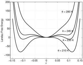
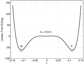
Figure 2: Non-convex free energy and its dependence on temperature

In the heart of the Ginzburg-Landau theory for the first order phase transformation in SMA, lies the free energy function defined as a non-convex function of the chosen order parameter for characterization of all the phases and variants (e.g., [10, 8, 12, 16]), which is defined as Equation (3). One example of the Landau free energy function is shown in Figure (2), for which the material and its physical parameters are given in section 5. It is shown clearly in the figure that the function has only one local minimum at high temperature ($\theta=280$K), which is associated with the only stable phase (austenite) in this case. At lower temperature ($\theta=210$K), there are two symmetrical local minima (marked with small gray rectangles), which are associated with martensite plus (P) and minus (M), respectively. For vibration damping purpose, it is always beneficial to make the SMA work at low temperature, so the hysteresis loop will be larger.

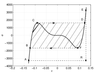
Figure 3: hysteretic behaviour and its damping effect caused by the non-convex free energy

The hysteretic behaviour and mechanical energy dissipation of the SMA rod at low temperature can be explained using its nonlinear constitutive relation as shown in Figure (3), which is obtained using the thermodynamical equilibrium condition [10]:

$$\sigma=\frac{\partial\mathcal{F}}{\partial\varepsilon}$$ (14)

For a given external loading, it will induce an internal stress and deformation in the SMA rod, part of the work done by the loading is stored in the rod via its deformation and can be calculated as:

$$W=\int_{\varepsilon_{s}}^{\varepsilon_{e}}(-\sigma\varepsilon)d\varepsilon,$$ (15)

where $\varepsilon_{s}$ and $\varepsilon_{e}$ are starting and ending strain values, respectively.

For pure elastic material, the stored energy can be released without loss when the external loading is removed, there is no mechanical energy dissipation. For thermo-mechanical coupling material, the stored energy is also obtainable when the loading is removed, but part of the input energy will be converted into thermal form and can not be fully released. If the material is insulated, its temperature will be slightly increased due to the input of mechanical energy. When viscous effects of the material are taken into account, the fraction of mechanical energy converted into thermal form will be larger, which means that dissipation of mechanical energy into thermal form is enhanced by viscous effects. But, compared to those due to mechanical hysteresis, all these energy dissipation are not remarkable.

The energy dissipation due to hysteresis can be presented schematically by considering the mechanical energy loss (converted from mechanical to thermal) in one cycle of loading [7, 12]. Assume that the loading process starts from point $A$ in Figure (3), and the load is continuously increased to point $E$. Then, the constitutive relation in this case will be the curve $ABCDE$, and the work done by the loading is represented by the area of $ABCDERA$. When the load is decreased from $E$ to $A$, the system will follow another constitutive curve $EDFBA$, and the work done by the rod is represented by the area of $EDFBARE$. There is a difference between the two areas, which is enclosed by the curve $BCDFB$ and hatched in the figure. This area represents the mechanical energy loss due to the hysteretic behaviour. At the same time, due to the thermo-mechanical coupling, the temperature of the material will be increased, as indicated by the source terms $k_{1}\theta\varepsilon\frac{\partial t}{\partial t}+\nu\left(\frac{\partial\varepsilon}{\partial t}\right)^{2}$ in the energy equation.

The physics behind this is that, when the external energy is applied to the SMA rod, part of the energy will be demanded by the material to convert itself from one variant (P) to another (M), as sketched in Figure (2). Both P and M are stable states, and have the same potential, so the material will not recover its previous configuration when the loading is removed. In this sense, the SMAs have plastic-like property. Part of the input mechanical energy is consumed just for converting the material from one variant to another (martensite phase transformation), and finally converted into thermal energy via the thermo-mechanical coupling. If one want to reverse the transformation, extra input energy is demanded.

4 Numerical Methodology

The constructed model for the vibration damping system given in Equation (13) is a strongly nonlinear coupled system. Experiences gained from the numerical experiments on similar problems shows that the development of an efficient algorithm is necessary for the numerical analysis of the model because standard iteration algorithms have difficulties to cope with the very strong nonlinearity [10, 12, 14, 16]. For the current problem, an additional difficulty is that the boundary conditions are system dependent. Indeed, we observe that the stress on the right end of the rod is a function of its displacement, velocity, and acceleration. In order to deal with these difficulties, the model is reduced to a differential-algebraic system and solved by using backward differentiation in time. The practical implementation is done similarly to [9, 14, 16]. Note, however, that here for the Chebyshev pseudo-spectral approximation, a set of Chebyshev points $\{x_{i}\}$ are chosen along the length direction as follows:

$$x_{i}=L\left(1-\cos(\frac{\pi i}{N})\right)/2,\quad i=0,1,\dots,N.$$ (16)

Using these nodes, $\varepsilon,v,\theta$, and $\sigma$ distributions in the rod can be expressed in terms of the following linear approximation:

$$f(x)=\sum_{i=0}^{N}f_{i}\phi_{i}(x),$$ (17)

where $f(x)$ stands for $\varepsilon,v,\theta$, or $\sigma$, and $f_{i}$ is the function value at $x_{i}$. Function $\phi_{i}(x)$ is the $i^{th}$ interpolating polynomial which has the following property:

$$\phi_{i}(x_{j})=\left\{\begin{array}[]{ll}1,&i=j,\\ 0,&i\neq j.\end{array}\right.$$ (18)

It is easy to see that the Lagrange interpolants would satisfy the the above requirements. Having obtained $f(x)$ approximately, the derivative $\partial f(x)/\partial x$ can be obtained by taking the derivative of the basis functions $\phi_{i}(x)$ with respect to $x$:

$$\frac{\partial f}{\partial x}=\sum_{i=1}^{N}f_{i}\frac{\partial\phi_{i}(x)}{\partial x}.$$ (19)

All these approximations are formulated in matrix form, for the convenience of actual programming implementation. For approximation to higher order derivatives, similar matrix form can be easily obtained. By substituting all the approximation into the DAE system, it will be recast into a set of nonlinear algebraic equations, which can be solved by Newton-Raphson iteration, following a similar way as done in Ref. ([9, 10, 14, 16]).

5 Numerical Experiments

Several different numerical experiments have been carried out to demonstrate the damping effects of hysteresis in the SMA rod induced by the phase transformations. All experiments reported in this section have been performed on a $\textrm{Au}_{23}\textrm{Cu}_{30}\textrm{Zn}_{47}$ rod, with length of 1$~{}cm$. Most of the physical parameters for this specific material can be found in the literature (e.g., [8, 14, 15, 16]), which are listed as follows for the sake of convenience:

$$k_{1}=480\,g/ms^{2}cmK,\quad k_{2}=6\times 10^{6}g/ms^{2}cmK,\qquad k_{3}=4.5\times 10^{8}g/ms^{2}cmK,$$

$$\theta_{1}=208K,\quad\rho=11.1g/cm{}^{3},\quad c_{v}=3.1274g/ms^{2}cmK,\quad k=1.9\times 10^{-2}cmg/ms^{3}K.$$

There are two coefficients, $k_{g}$ and $\nu$, are not easy to find its value. Normally, $k_{g}$ is very small and here we take it as $5$ by referring to the value indicated in Ref.([10, 11]). The value of $\nu$ is take as $10$, with the same unit system. To demonstrate the damping effects of the SMA rod, we set $\mu_{m}=k_{m}=0$ in Equation (13). Then, only the force from the SMA rod is taken into account.

For all numerical experiments, the initial conditions for the rod are chosen as $\theta=210^{o}$, $\varepsilon=0.115$, $u=v=0$, the simulation time span is $[0,4]ms$, and $40$ nodes have been used for the Chebyshev approximation.

In the first experiment reported here, the parameter $m/\beta$ is chosen as $200~{}(g/cm^{2})$ and the initial value of $v_{m}$ is chosen $-3~{}(cm/ms)$. The numerical results are presented in Figure (4).

From the upper left plot it can be observed that the velocity of the block is damped effectively, and gradually the velocity tends to a small value. The entire damping process can be roughly divided into two stages. The first stage is $t\in[0,2.6]ms$ in which the damping is more effective since the vibration energy is still large enough to switching the whole SMA rod between martensite plus and minus at low temperature (martensite phase transformation). While in the the second stage, the contribution from phase transformation becomes weaker and finally fades because the temperature is raised, the mechanical energy is also dissipated and not large enough to induce phase transformation. The motion of the rod finally becomes a thermo-mechanical vibration without phase transformations at the end of the simulation. The strain distribution, presented in the lower right part of the plot, shows this clearly. In the lower left plot, we present the average temperature of the rod, which could be regarded as a measurement of thermal energy. Since insulation thermal conditions are used and there is no thermal dissipation included in the model, the temperature is increased rapidly when there is phase transformation induced because the large change rate of strain, and much slower when there is no transformation. This observation indicates that the conversion of mechanical energy into thermal form is much faster when phase transformation takes place. The oscillation of average temperature is caused by the phase transformation and thermo-mechanical coupling.

To analyze the damping effects further, we have increased the initial vibration energy to $m/\beta=500$. The numerical results for this case are presented in Figure (5), in a similar way as those in Figure (4). It is seen from the strain plot that the whole rod is switched between compressed ($\varepsilon<0$) and stretched ($\varepsilon>0$) states in the entire simulation range, and $v_{m}$ is decreased continuously. This strain switching causes the temperature oscillation. The dissipation of mechanical energy is faster at the beginning and becomes slower after a while in the simulation, which is indicated by the velocity plot (consider that mechanical energy is proportional to the square of velocity). This is due to the fact that phase transformation only takes place in a short period in which the rod temperature is still low, which can be roughly read as $[0,1.4]ms$ form the temperature plot, in which the temperature increases faster. Afterwards, there is no phase transformation since the rod is at high temperature state and the motion becomes thermo-mechanical vibration again. This observation leads to same conclusion that phase transformation contribute most to the damping effects (energy conversion).

To show the damping effects contributed from the viscous effects and thermo-mechanical coupling, the last numerical example presented here has been dealing with the analysis of the damping effects when there is no phase transformation induced in the SMA rod at all. For this purpose, the parameters are chosen as $m/\beta=20$, and initial velocity $v_{m}=-1$ such that the input mechanical energy is too small to induce phase transformation, and the simulation time span is also extented to $[0,20]$ms to capture the long time behaviour since the mechanical energy dissiption might be much slower. For the simulation of damping effects contributed from thermo-mechanical coupling alone, the parameter is set $\nu=0$ (no viscous effects), and the numerical results are presented on the left column of Figure (6), by plotting the evolution of mass block velocty (top) and average temperature of the SMA rod (bottom). It indicates that the coupling alone does contribute to damping effects, the mechanical energy stored via the mass block motion is finally converted into thermal form, and increase the SMA rod temperature slightly. But, the dissipation of mechanical energy into thermal form is rather slow, there are still oscillations at the end of the simulation. In order to include the contribution from viscos effects, now the viscosity parameter is set $\nu=20$, numerical results are presented on the right column similarly in the figure. It is shown clearly that when viscous effects are incorportate (right), the conversion of energy due to thermo-mechanical coupling is enhanced, the the system is already at rest at $t=15$ms. In both case, the oscillation of velocity and average temperature has a series of peaks, which indicates a complicate nature of the thermo-mechanical energy conversion.

In all these three numerical experiments, the energy conversion between mechanical and thermal form due to thermo-mechanical coupling is well captured. It is shown that when the phase transformation is induced, the vibration damping is remarkabley enhanced because the energy conversion is enhanced. Because there is no heat loss considered here, the average temperature of the rod increases continuously. It is clear that if the SMA damper is controlled at low temperature by external efforts, it will be an effective damper.

6 Conclusions

In this paper, we constructed a mathematical model for vibration damping of a mass block connected with a SMA rod. We employed the modified Ginzburg - Landau theory for the mathematical modelling of the SMA rod to capture the phase transformation and thermo-mechanical coupling. The model for the vibration of the block is coupled with the dynamics of the SMA rod by adjusting the boundary conditions. The model is then numerically analyzed and the damping characteristics of the SMA rod due to the first order martensite phase transformation are investigated. It is shown that the vibration can be effectively damped, if the first order phase transformation is induced.

Figure 1: Vibration damping of a mass block connected to a shape memory alloy rod.

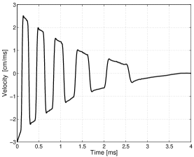
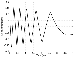
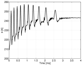
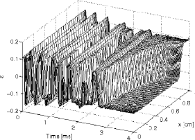
Figure 4: Damping effect of a SMA rod involving mechanically induced phase transformations

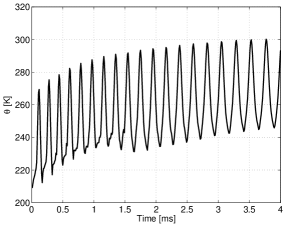
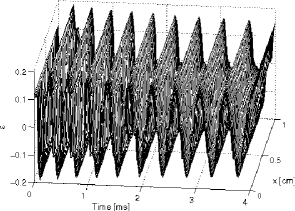
Figure 5: Damping effect of a SMA rod with large initial vibration energy

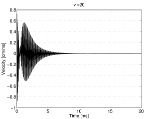
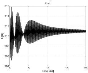
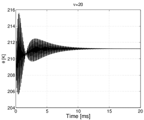
Figure 6: Effects of internal friction on damping performance of shape memory alloy rods (no phase transformations)

References

- [1] Birman,V., Review of mechanics of shape memory alloys structures, Appl.Mech.Rev. 50 (1997) 629-645.
- [2] Song, G., Ma, N., and Li, H. N., Application of shape memory alloys in civil structures, Engineering Structures 28 (2006) 1266 - 1274.
- [3] Juan, J. S., and No, M. L., Damping behaviour during martensite transformation in shape memory alloys, Journal of Alloys and Compounds 355 (2003) 65 - 71.
- [4] Humbeeck, J. V., Damping capacity of thermoelastic martensite shape memory alloys, Journal of Alloys and Compounds, 355 (2003) 58 -64
- [5] Piedboeuf, M. C., Gauvin, R., and Thomas, M., Damping behaviour of shape memory alloys: Strain amplitude, frequency and temperature effects. Journal of Sound and Vibration 214 (5) (1998) 885 - 901
- [6] Chen, Y.C., Lagoudas, D. C., Impact induced phase transformation in shape memory alloys, Journal of the Mechanics and Physics of Solids, 48 (2000) 275 - 300.
- [7] Masuda, A., and Noori, M. Optimisation of hysteretic characteristics of damping devices based on pseudoelastic shape memory alloys. Inter. J. Nonlinear Mech. 37 (2002) 1375-1386.
- [8] Falk, F., Model free energy, mechanics, and thermomechanics of shape memory alloys. Acta Metallurgica, 28, (1980) 1773-1780.
- [9] Matus, P., Melnik, R., Wang, L., Rybak, I.: Application of fully conservative schemes in nonlinear thermoelasticity: Modelling shape memory materials. Mathematics and Computers in Simulation. Mathematics And Computers in Simulation 65 4-5 489-509
- [10] Bunber, N., Landau-Ginzburg model for a deformation-driven experiment on shape memory alloys. Continuum Mech. Thermodyn. 8 (1996) 293-308.
- [11] Bubner, N., Mackin, G., and Rogers, R. C., Rate depdence of hysteresis in one-dimensional phase transitions, Comp. Mater. Sci., 18 (2000) 245 - 254.
- [12] Koucek, P, Reynolds, D. R., and Seidman, T. I., Computational modelling of vibration damping in SMA wires, Continuum Mech. Thermodyn. 16 (2004) 495 - 514.
- [13] Bales, G.S. and Gooding, R.J., Interfacial dynamics at a 1st-order phase-transition involving strain dynamic twin formation. Phys. Rev. Lett.,67, (1991) 3412.
- [14] Melnik, R., Roberts, A., Thomas, K.: Phase transitions in shape memory alloys with hyperbolic heat conduction and differential algebraic models. Computational Mechanics 29 (1) (2002) 16-26.
- [15] Niezgodka, M., Sprekels, J.: Convergent numerical approximations of the thermomechanical phase transitions in shape memory alloys. Numerische Mathematik 58(1991) 759-778.
- [16] Wang, L.X, and R.V.N.Melnik, Thermomechanical waves in SMA patches under small mechanical loadings. in Lecture Notes in Computer Science 3039, (2004), 645-652.
- [17] Chaplygin, M. N., Darinskii, B. M., and Sidorkin, A. S., Nonlinear Waves in Ferroelastics, Ferroelectrics, 307 (2004) 1-6.
- [18] Abeyaratne, R;, and Knowles, J. K., On a shock-induced martensitic phase transition, J. Appl. Phys. 87 (2000), 1123 - 1134.