Generic Global Constraints based on MDDs

Abstract

Constraint Programming (CP)[1] has been successfully applied to both constraint satisfaction and constraint optimization problems. A wide variety of specialized global constraints provide critical assistance in achieving a good model that can take advantage of the structure of the problem in the search for a solution. However, a key outstanding issue is the representation of ’ad-hoc’ constraints that do not have an inherent combinatorial nature, and hence are not modelled well using narrowly specialized global constraints. We attempt to address this issue by considering a hybrid of search and compilation. Specifically we suggest the use of Reduced Ordered Multi-Valued Decision Diagrams (ROMDDs) as the supporting data structure for a generic global constraint. We give an algorithm for maintaining generalized arc consistency (GAC) on this constraint that amortizes the cost of the GAC computation over a root-to-leaf path in the search tree without requiring asymptotically more space than used for the MDD. Furthermore we present an approach for incrementally maintaining the reduced property of the MDD during the search, and show how this can be used for providing domain entailment detection. Finally we discuss how to apply our approach to other similar data structures such as AOMDDs and Case DAGs. The technique used can be seen as an extension of the GAC algorithm for the regular language constraint on finite length input [2].

1 Introduction

Constraint Programming (CP)[1] is a powerful technique for specifying Constraint Satisfaction Problems (CSPs) based on allowing a constraint programmer to model problems in terms of high-level constraints. Using such global constraints allows easier specification of problems but also allows for faster solvers that take advantage of the structure in the problem.

The classical approach to CSP solving is to explore the search tree of all possible assignments to the variables in a depth-first search backtracking manner, guided by various heuristics, until a solution is found or proven not to exist. One of the most basic techniques for reducing the number of search tree nodes explored is to perform domain propagation at each node. In order to get as much domain propagation as possible we wish for each constraint to remove from the variable domains all values that cannot participate in a solution to that constraint. This property is known as Generalized Arc Consistency (GAC).

It is only possible to achieve GAC for some types of global constraints in practice, as a global constraint can model NP-hard problems making it infeasible to achieve GAC. The use of global constraints can significantly reduce the total number of constraints in the model, which again improves domain propagation if GAC or other powerful types of consistency can be enforced. However, in typical CSPs there are many constraints that lie outside the domain of the current global constraints. Such constraints are typically represented as a conjunction of simple logical constraints or stored in tabular form. The former can potentially reduce the amount of domain propagation, while the tabular constraints typically takes up too much space for all but the most simple constraints, and hence it is also computationally expensive to achieve GAC.

The aim of this paper is to introduce a new generic global constraint type for constraints on finite domains based on the approach of compiling an explicit, but compressed, representation of the solution space of as many constraints as possible. To this end we suggest the use of Multi-Valued Decision Diagrams (MDDs).

It is already known how to perform GAC in linear, or nearly linear time in the size of the decision diagram for many types of decision diagrams including MDDs [3, 4, 5]. However, compact as decision diagrams may be, they are still of exponential size in the number of variables in the worst case. In practice their size is also the main concern, even when they do not exhibit worst case behavior. Applying the static GAC algorithms at every step of the search is therefore likely to cause an unacceptable overhead in many cases.

To avoid the overhead it is essential to avoid repeating computation from scratch at each step and instead use an algorithm that amortizes the cost of the GAC computation over a number of domain propagation steps. In this paper we introduce such an algorithm using ideas from [2]. The paper is structured as follows. In Section 1.1 we discuss in some detail how are our contributions are related to those contained in [2] as well as briefly describe other related results. In Section 2 we describe the functionality required from the global constraint we are presenting and the setup in which it can be used. In Section 3 we describe how the technique from [2] can be applied to a simplified MDD. We then move on to show how we can extend that approach to handle long edges in MDDs in Section 4. In Section 5 we present results on maintaining the reduced property of the constraint during a search. Based on this we show how domain entailment can be detected in Section 5.3. Finally we discuss how our approach can be applied to other data structures that are similar to MDDs, such as AOMDDs and Case DAGs in Section 7.

1.1 Related Work

The concept of compiling an explicit, but compact, representation of the solution space of a set of constraints has previously been applied to obtain backtrack-free configurators for many practical configuration problems [6]. In this case Binary Decision Diagrams (BDDs) [3] are used for representing the solution space. However, it is well known that BDDs (and MDDs) are not capable of efficiently representing prominent constraints such as the AllDifferent constraint [7].

A regular language constraint for finite sequences of variables is introduced in [2]. It uses a DFA to represent the valid inputs where the input is limited to be of length $n$. Since the constraint considers a finite number of inputs, these can be mapped to $n$ variables, and GAC can be enforced according to the domains of these variables. To this end the cycles in the DFA are ’unfolded’ by taking advantage of the fact that the input is of a finite length. The resulting data structure has size $O(nd_{max}q)$ where $q$ is the number of states in the original DFA and $d_{max}$ the size of the largest variable domain. A bounded incremental GAC algorithm with complexity linear in the number of data structure changes is also presented. Since this regular global constraint is defined on a finite length input, it can be used as a generic constraint. In fact, we note that there is a strong correspondence between the unfolded DFA and a simplified MDD representing the same constraint. However, there are some important theoretical and practical reasons for using fully reduced MDDs when the goal is a generic global constraint. Below we summarize our contributions and highlight the differences compared to using the regular constraint in the role of a generic global constraint.

• Firstly, DFAs do not allow skipping inputs, even for states where the next input is irrelevant. Skipping input variables in this manner is part of the reduce steps for BDDs, and if it is used in MDDs it requires alterations to the GAC algorithm. We give a modified algorithm to handle this. In some cases allowing the decision diagram to skip variables can give a significant reduction in size. A very simple example is a constraint specifying that the value $v$ must occur at least once for one of the variables $x_{1},\ldots,x_{n}$ each having the same domain of size $d$. In an MDD that does not allow skipped variables (such as an unfolded DFA) this requires $\Omega(n^{2}d^{2})$ nodes compared to $O(nd)$ nodes if we allow skipped variables in the MDD.

• Secondly, BDDs are normally kept reduced during operations on the BDDs. This allows subsequent operations to run faster and also shows directly if the result is the constant true function. We present an approach that can dynamically reduce the MDD without resorting to scanning the entire live part of the data structure, and which also allows us to detect domain entailment [8]. Domain entailment detection can be critical for the performance of a CSP solver, as it can save a potentially exponential number of exectutions of the GAC algorithm. The technique described in [2] does not provide dynamic reduction or domain entailment detection.

  The suggestion in [2] is to minimize the DFA only once at the beginning (thereby also minimizing the initial ’unfolded’ DFA) which would correspond to reducing the MDD prior to the search, and does not provide any form of entailment detection. The problem of efficient dynamic minimization is not discussed in [2] and would seem to require a technique similar to the one we present in this paper for obtaining dynamic reduction of the MDD constraint.

• Thirdly, we cover how the GAC algorithm can be adapted to operate on other decision diagram style data structures such as AOMDDs [4] and Case DAGs [9].

Finally, from a practical perspective it is not a good idea to first construct a DFA and then unfold it. It is more efficient to use a BDD package to construct an ROBDD directly, as efficient BDD packages [10, 11] with a focus on optimizing the construction phase have already been developed driven by needs in formal verification [12]. Specifically the use of BDDs for the construction gives access to the extensive work done on variable ordering (see for example [13, 14, 15]) for BDDs. Once an ROBDD is constructed it can then easily be converted into the desired MDD.

Another related result is [16] in which it is discussed how to maintain Generalized Arc Consistency in a generic global constraint on binary variables based on a BDD. Their technique differs from the straightforward DFS scanning technique by using shared good/no-good recording and a simple cut-off technique to in some cases reduce the amount of nodes visited in a scan. Their technique can be adapted for non-binary variables, but the cut-off technique lose merit if the MDD is to be reduced dynamically and becomes much less efficient as the domains increase in size. Hence their techniques do not apply when the intention is to collect sets of small constraints into a few larger MDD constraints.

1.2 Notation

In this paper we consider a CSP problem $\textit{CP}(X,D,F)$, where $X=\{x_{1},\ldots,x_{n}\}$ is the set of variables, $F$ the set of constraints on the variables in $X$ and $D=\{D_{1},\ldots,D_{n}\}$ is the multi-set of variable domains, such that the domain of a variable $x_{i}$ is $D_{i}$. We use $d_{i}=|D_{i}|$ to denote the size of domains and $d_{max}=\max\{d_{i}\mid x_{i}\in X\}$ to denote the largest domain. A single assignment is a pair $(x_{i},v)$ where $x_{i}\in X$ and $v\in D_{i}$. The assignment $(x_{i},v)$ is said to have support in a constraint $F_{k}$, iff there exists a solution to $F_{k}$ where $x_{i}$ is assigned $v$. If a single assignment ($x_{i},v$) for which $v\in D_{i}$ has support in a constraint $F_{j}$, $v$ is said to be in the valid domain for $x_{i}$ respective to $F_{j}$ , denoted $\textrm{VD}_{i}(F_{j})$. If for all variables $x_{i}$ and a constraint $F_{j}$ it is the case that $D_{i}=\textrm{VD}_{i}(F_{j})$ then $F_{j}$ is said to fulfill the property of Generalized Arc Consistency (GAC). A partial assignment $\rho$ is a set of single assignments to distinct variables, and a full assignment is a partial assignment that assigns values to all variables.

We now define an MDD constraint belonging to a specific CSP.

Definition 1 (Ordered Multi-Valued Decision Diagram (OMDD))

An Ordered Multi-Valued Decision Diagram (OMDD or just MDD) for a CSP CP is a layered Directed Acyclic MultiGraph $G(V,E)$ with $n+1$ layers (some of which may be empty). Each node $u$ has a label $l(u)\in\{1,\ldots,n+1\}$ corresponding to the layer in which the node is placed, and each edge $e$ outgoing from layer $i$ has a value label $v(e)\in D_{i}$. Furthermore we use $s(e)$ and $d(e)$ to denote respectively the source and destination layer of each edge $e$ .

The following restrictions apply:

• There is exactly one node $u$ such that $l(u)=\min\{l(q)\mid q\in V\}$ denoted root.

• There is exactly one node $u$ such that $l(u)=n+1$ denoted terminal.

• For any node $u$, all outgoing edges from $u$ have distinct labels.

• All nodes except terminal has at least one outgoing edge.

• For all $e\in E$ it is the case that $s(e)<d(e)$.

We will use $V_{i}=\{u\in V\mid l(u)=i\}$ to denote the nodes of layer $i$ and $E_{i}=\{e\in E\mid s(e)=i\}$ to denote the set of edges originating from layer $i$. Furthermore we define

$$P_{u}=\{(p,v)\mid\exists e=(p,u)\in E:v(e)=v\}$$

and

$$C_{u}=\{(c,v)\mid\exists e=(u,c)\in E:v(e)=v\}$$

That is, $P_{u}$ corresponds to the incoming edges to $u$, and $C_{u}$ corresponds to the outgoing edges of $u$. Given layers $i>j>k$, we say that $i$ is a later layer than $j$ and that $k$ is an earlier layer than $j$.

Definition 2 (Solution to an MDD)

A full assignment $\rho$ is a solution to a given MDD iff there exists a path $Q=(e_{1},\ldots,e_{j})$ from root to terminal such that for each $(x_{i},v)\in\rho$ at least one of the following conditions hold:

• $\exists e\in Q$ such that $s(e)=i$ and $v(e)=v$

• $l(root)>i$

• $\exists e\in Q$ such that $s(e)<i<d(e)$.

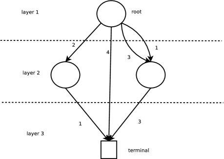
An edge $e$ such that $s(e)+1<d(e)$, as in the third condition in the above definition, is called a long edge and is said to skip layer $s(e)+1$ to $d(e)-1$. It it is worth noting that one long edge can represent many partial assignments.

Definition 3 (Reduced OMDD)

An MDD is called uniqueness reduced iff for any two distinct nodes $u_{1},u_{2}$ at any layer $i$ it is the case that $C_{u_{1}}\not=C_{u_{2}}$. If it is furthermore the case for all layers $i\in\{1,\ldots,n\}$ that no node $u_{1}$ in layer $i$ exists with $d_{i}$ outgoing edges to the same node $u_{2}$, the MDD is said to be fully reduced.

The above definitions are just the straightforward extension of the similar properties of BDDs[3]. Fully reduced MDDs retain the canonicity property of reduced BDDs, that is, for each ordering of the variables there is exactly one fully reduced MDD for each Boolean constraint on $n$ discrete domain variables. An example reduced MDD is shown in Figure 1.

Figure 1: The above figure shows an example MDD that is fully reduced. Assuming $D_{1}=\{1,2,3,4\}$ and $D_{2}=\{1,2,3\}$, it represents the binary constraint with solutions { (1,3),(2,1), (3,3),(4,1),(4,2),(4,3) }.

2 Searching with an MDD

In this paper we consider a backtracking search for a solution to a conjunction of constraints, at least one of which is an MDD. To simplify the complexity analysis, we assume that the search branches on the domain values of each variable in some specified order and that full domain propagation takes place after each branching. The process of branching and performing full domain propagation we will refer to as a phase. For our proposed global constraint we refer to performing domain propagation on it as a single step. As such, one phase may contain many steps depending on how many iterations it takes until none of the constraints are able to remove any further domain values. In order to be useful in this type of CSP search, an implementation of the MDD constraint needs to supply the following functionality:

• Assign($x,v$)

• Remove($(x_{1},v_{1}),\ldots,(x_{k},v_{k})$)

• Backtrack()

The Assign operation restricts the valid domain of $x$ to $v$ and is used to perform branchings. The Remove operation corresponds to domain restrictions occurring due to domain propagation in the other constraints. The Backtrack operations undoes the last Assign operation and all Remove operations that has occurred since, effectively backtracking one phase in the search tree. For the implementation of Backtrack we will simply push data structure changes on a stack, so that they can be reversed easily when a backtrack is requested. This very simple method ensures that a backtrack can be performed in time linear in the number of data structure changes made in the last phase. For all the dynamic data structures considered in this paper the space used for this undo stack will be asymptotically bounded by the time used over a root-to-leaf path in the search tree. Furthermore, in all the cases studied in this paper, Assign($x_{i},v$) is just as efficiently implemented as a single call to Remove($\{(x_{i},v_{j})\mid v_{j}\in D_{i}\setminus\{v\}\}$). Therefore we will only discuss the implementation of Remove.

3 Calculating the change in valid domains

In the following we will say that an edge $e$ is valid iff there exists a path in the MDD, corresponding to a solution to the MDD under all restrictions applied so far, such that $e$ is part of the path. We furthermore say that a node is valid if it is root or has at least one valid incoming and outgoing edge. A crucial element in computing the valid domains in an MDD is that of a supporting edge. A valid edge $e\in E$ supports a single assignment $(x_{i},v)$, if $s(e)=i$ and $v(e)=v$ or if $s(e)<i<d(e)$. Note that $v\in D_{i}$ iff there exists an edge $e$ supporting the assignment $(x_{i},v)$. We say that a node $u$ supports a value $v$ if there exists an edge $(u,c)$ supporting $(x_{l(u},v)$ for some $c$.

In this section we will show how the approach from [2] can be used for maintaining the valid domains of a simplified MDD. We will temporarily assume that the OMDD we operate on is initially Uniqueness Reduced, but not fully reduced, in fact we will assume that all outgoing nodes from a node in layer $i$ lead to nodes in layer $i+1$ (and hence also that $l(root)=1$).

3.1 Tracking support

Valid domains are maintained by tracking the loss of supporting edges for each possible assignment as restrictions of the form $x_{i}\not=v$ are applied. The application of a restriction $x_{i}\not=v$ immediatly invalidates all edges originating from layer $i$ with label $v$. We need to compute what further supporting edges are invalidated as a consequence and determine if any assignments have lost their supporting edges.

We track the set of supporting edges by storing a set of sets $S$, such that for every possible single assignment $(x_{i},v)$ where $x_{i}\in X$ and $v\in D_{i}$ there exists a set $s_{i,v}\in S$ containing all the nodes and the corresponding edges that gives support to the single assignment $(x_{i},v)$. In maintaining $S$ we learn immediately when a single assignment $(x_{i},v)$ no longer has support, as $s_{i,v}$ will be empty. Note that the space needed for the support lists is only $O(|E|)$. The approach to maintaining $S$ is very simple. To apply a restriction $x_{i}\not=v$, we first invalidate all edges supporting this assignment. We then check if this has made any nodes invalid, and if so invalidate their edges, continuing recursively.

3.2 Performing Remove

The above support tracking technique is implemented as the procedures Remove and RemoveEdge shown in Figure 2. The remove operation is performed by, for each single assignment $(x_{i},v)$ to be removed, visiting all nodes that offer support for $(x_{i},v)$. On each such node the update procedure RemoveEdge is used to remove the corresponding invalidated edge while maintaining $S$ and the valid domains.

3.3 Complexity

The RemoveEdge operation can easily be supported in $O(1)$ time per call using $O(|E|)$ space using just linked lists for the support sets and pointers from each edge to their corresponding support list entry.

Consider a path in the search tree implicitly represented by the branching search. We will here and in the following describe the complexity of the presented algorithms as the complexity over such a root-to-leaf path in the search tree. Since each edge can only be removed once during this part of the search we obtain the following result:

Lemma 1

Consider any root-to-leaf path in the search tree. Then the total number of calls to RemoveEdge is at most $O(|E|).$

4 Skipping input variables

We have so far obtained a very efficient GAC algorithm for a simplified MDD data structure by simply applying the technique from [2] to our MDD constraint. However, the algorithm described so far does not allow the MDD to be fully reduced. Specifically it does not take long edges or the possibility that the root is not placed in layer $1$ into consideration. If the root is in a layer $i>1$, we will simply add a long edge that skips layer $1$ to $i-1$, such that we only need to deal with long edges.

4.1 Handling long edges

For the purpose of valid domains computation, the important observation is that if a valid long edge exists skipping layer $i$ to $j$, then all available domain values for the corresponding variables are also supported. For static valid domains computation [5] these variables are found by for each level finding the longest outgoing edge. Given this information it is simple to list the variables which have full support due to a long edge skipping over their layer in time $O(n)$. We obtain a dynamic equivalent of this algorithm by maintaining the length of the longest long edges originating from each level. Additionally each long edge $e$ is placed in the support list of $(x_{s(e)},v(e))$, as if it was a regular edge. In order to track the longest outgoing edge of each level we will maintain the set $L$ of distinct intervals $[i,j]$ such that there exists at least one long edge skipping layers $i$ to $j$. In order to detect when a skipped interval should be removed from $L$, we for each skipped interval $[i,j]\in L$ maintain a counter $l_{i,j}$, giving the number of long edges skipping exactly the layers $i$ to $j$. A long edge $e$ skipping layer $i$ to $j$ can no longer support the skipping of the interval $[i,j]$ iff $e$ is invalidated. In this case $l_{i,j}$ is decremented, and in case $l_{i,j}=0$ the skipped interval $[i,j]$ is removed from $L$. Note that we do not perform any update if a Remove call actually ’cuts’ a long edge into two parts. This means that we allow the intervals to support values that are invalid. However, the only invalid values supported in this way are those that are given as arguments to Remove, and have therefore already been removed from the valid domain values by another constraint.

Recall that our goal is to maintain the longest outgoing edge from each layer in the MDD. Using the above we can do this simply by maintaining a max-priority queue for each level $i$ over the the set of skipped intervals of the form $[i,j]$, for some $j$, using $j$ as key. Assuming the priority queue supports reporting the maximum in time $O(1)$ we can obtain the required table in $O(n)$ time. It should now also be clear why we build the priority queue over the distinct intervals instead of all the intervals represented by long edges. Had we used the long edges directly, all edge deletions would require a delete operation on the priority queue, while we now only need a delete operation when a distinct interval no longer has any supporting long edges. The algorithm is given in Figure 2 and the following lemma gives its complexity.

• $\textnormal{Init}()$
     1Initialize each support list $s_{i,v}$ 2$L\leftarrow$ the set of intervals skipped by at least one long edge 3$l_{i,j}\leftarrow$ the number of long edges skipping exactly layer $i$ to $j$ 4$D^{s}_{i}\leftarrow$ the values for $x_{i}$ supported by the support lists 5$U\leftarrow\{1,\ldots,n\}$ 6Remove$(\emptyset)$ $\rhd$ Initial domain propagation

• $\textnormal{Remove}(R)$
     1for each $(x_{i},v)\in R$ 2 dofor each $(u,c)\in s_{i,v}$ $\rhd$ Remove edges supporting $(x_{i},v)$ 3 $\textnormal{RemoveEdge}(u,c,v)$ 4$U^{\prime}\leftarrow$ union of the intervals in $L$ 5for each $l\in U\setminus U^{\prime}$ $\rhd$ Layer $l$ is no longer skipped by a long edge 6 do$D_{l}=D^{s}_{l}$ 7 if $D_{l}=\emptyset$ 8 then Constraint failed 9$U\leftarrow U^{\prime}$

• $\textnormal{RemoveEdge}(u,c,v)$
      1$s_{l(u),v}\leftarrow s_{l(u),v}\setminus\{(u,c)\}$ 2if $s_{l(u),v}=\emptyset$ $\rhd$ $(x_{l(u)},v)$ no longer supported in support lists 3 then $D^{s}_{l(u)}\leftarrow D^{s}_{l(u)}\setminus\{v\}$ 4$C_{u}\leftarrow C_{u}\setminus\{(c,v)\}$ 5$P_{c}\leftarrow P_{c}\setminus\{(u,v)\}$ 6if $l(c)-l(u)>1$ $\rhd$ If the removed edge is a long edge 7 then decrement $l_{l(u)+1,l(c)-1}$ 8 if $l_{l(u)+1,l(c)-1}=0$ 9 then $L\leftarrow L\setminus\{[l(u)+1,l(c)-1]\}$ 10if $C_{u}=\emptyset$ $\rhd$ $u$ has no outgoing edges 11 then for each $(p,v^{\prime})\in P_{u}$ $\rhd$ Remove incoming edges 12 do$\textnormal{RemoveEdge}(p,u,v^{\prime})$ 13if $P_{c}=\emptyset$ $\rhd$ $u$ has no incoming edges 14 then for each $(c^{\prime},v^{\prime})\in C_{c}$ $\rhd$ Remove outgoing edges 15 doRemoveEdge$(c,c^{\prime},v^{\prime})$

Figure 2: Remove calls RemoveEdge for each edge that must be removed due the restrictions in $R$. Afterwards it recomputes the layers supported by long edges $L$ and updates the domains accordingly. RemoveEdge takes as input an invalid edge in form of the source node $u$, the destination node $c$ and the corresponding value label $v$. It then moves from the invalid edge downwards in depth first manner as long as there are nodes being invalidated due to lacking valid incoming edges. If the node $u$ has no more outgoing edges it propagates upwards, removing nodes that have no more outgoing edges. Recall that $P_{u}$ corresponds to the incoming edges of $u$ and $C_{u}$ to the outgoing edges. For each edge it removes it decrements the counter of the corresponding skipped interval and updates $L$ if needed.

Lemma 2

On a root-to-leaf in the search tree the complexity of the longest-outgoing-edge based approach is bounded by $O(|E|+n^{2}\lg\lg n+n^{2}d_{max})$.

Proof

As previously, the actual time for handling normal edges is at most $O(|E|)$. Each interval can only be removed once, and each such deletion costs $O(\lg\lg|L|)$ using a VEB-based priority queue [17]. Finally we spent $O(n)$ time per step to compute the table of longest outgoing edges and compute the variables covered by long edges. In total this yields a complexity over a root-to-leaf path in the search tree of $O(|E|+|L|\lg\lg|L|+tn)$, where $t$ is the number of steps. Since there can at most be $O(n^{2})$ distinct long edge intervals and $nd_{max}$ steps this yields $O(|E|+n^{2}\lg\lg n+n^{2}d_{max})$.

We believe that for most practical applications of the MDD constraint the above complexity will be completely dominated by the $|E|$ factor, and hence that the addition of long edges result in no significant performance impact. As an alternative solution we can use the dynamic interval union data structure (DIU) presented in [18] to store the intervals. Using this data structure it is possible to obtain a complexity of $O(|E|+n^{2}\lg n+nd_{max})$ [19]. However for practical applications, the longest-outgoing-edge approach using a simple binary heap is most likely preferable (yielding $O(|E|+n^{2}\lg n+n^{2}d_{max})$) due to the simple implementation and low overhead.

5 Maintaining the reducedness property

In the above we do not take steps to maintain the uniqueness reduced property of the MDD when we update the data structure. This forfeits a chance for a large speed-up. If a reduction at an early search node $s$ would lead to large reduction in the size of the data structure all descendant search node of $s$ (of which there can be an exponential number) would benefit from working on a much smaller data structure. As an example of the effect of dynamic reduction consider the simple constraint $f$ encoding the rule $x_{1}\leq x_{2},x_{1}\leq x_{3}\ldots,x_{1}\leq x_{j}$ with domains $D_{i}=\{1,\ldots,k\}$ for some constant $k$. Let $MDD(f)$ be the MDD representing $f$ and let $f_{v}=f\land x_{1}=v$. Now consider the removal of the value $1$ from the domain $x_{2},\ldots,x_{j}$ (as could be induced by an external AllDifferent constraint). With this restriction $MDD(f_{1})$ becomes equivalent to $MDD(f_{2})$ and can be merged, reducing the size of the MDD required to store the constraint with a constant factor. If the value $2$ is lost next then a further constant fraction of the MDD can be removed due to the reduce step as $f_{1}=f_{2}$ now becomes equivalent to $f_{3}$. This is of course a very simplistic constraint easily propagated using other methods, but if we consider the conjunction of the constraint with another constraint, the example still applies in many cases, especially if the new constraint does not depend on the value of $x_{1}$. One example of such an additional constraint is $\forall i\in[2,j-1]:x_{i}\not=x_{i+1}$. Note that if we ensure the uniqueness reduced property the MDD will be fully reduced according to the original domains throughout the search (assuming it is fully reduced initially), since there is no risk that new long edges will be created when we only perform domain restrictions. We therefore first discuss how to ensure the uniqueness reduced property and then describe the addition necessary in order to obtain full reduction according to the current domains.

5.1 Dynamic reduction

Assuming that the MDD is uniqueness reduced for all layers later than layer $i$, a node $u$ in layer $i$ becomes redundant iff at least one of its outgoing edges are modified such that $C_{u}=C_{q}$ for some node $q$ in layer $i$. This redundancy can be removed by merging the redundant nodes. Two redundant nodes $u$, $q$ are merged by removing $u$ and redirecting all edges ending in $u$ to $q$ or vice versa. In the first case we say that $u$ is the subsumee, and $q$ the subsumer. Note that a merger can give rise to redundancies in earlier layers, but not in later layers. We will therefore dynamically reduce the MDD by maintaining maintain a set of ’dirty’ nodes that need to be checked for redundancy during the operation of Remove. Afterwards we check the dirty nodes for redundancy in a bottom-up manner, ensuring that later layers are uniqueness reduced, before earlier layers are considered.

5.1.1 Redundancy detection

In order to efficiently check whether a given node has become redundant we will for each node maintain a hash signature computed based on the node’s level and outgoing edges. Using this signature and a hashtable we can discover nodes that become redundant. Some care must be take to ensure that the signature can be updated in $O(1)$ time when an edge changes. This can be ensured using a variation of vector hashing [20], which we describe in [19]. We would like to stress that vector hashing has a very low overhead, and has been shown to be competitive in practice. Additionally, to ensure that collisions in the hash table do not give rise to expensive comparisons between the outgoing edges of two nodes, we utilize the technique of generating a hash signature longer than necessary to index the hash table. Using this technique nodes need only to be compared when their full signature matches, even though they reside in the same bucket in the hash table. In this way it is possible to ensure that inserting a node which is not redundant takes expected time $O(1)$ and that insertion of a redundant node $u$ takes expected time $O(|C_{u}|)$. A detailed description can be found in [19].

5.1.2 Merging nodes

Given two nodes $u_{1}$ and $u_{2}$ to merge we always designate the one with the largest number of parents as the subsumer in order to reduce the total cost of the merge operations. An edge $e$ is only redirected when its end-point $c$ is subsumed. Since this only happens when another node of larger in-degree becomes identical to $c$ the in-degree required to cause $e$ to be redirected must at least double each time $e$ is moved. Hence an edge can only be moved $\lceil\lg(|V|)\rceil$ times as $|V|$ is an upper bound on the in-degree of a node. Note that this is a very simple and classic greedy strategy that incurs no significant overhead.

5.1.3 Complexity of dynamic reduction

Lemma 3

The expected time spent over a root-to-leaf path in the search tree by Remove on reducing the MDD is $O(|E|\lg|V|)$.

Proof

Since each edge can only be redirected $\lceil\lg(|V|)\rceil$ times the total cost of redirecting edges is $O(|E|\lg|V|)$. Checking and discovering a redundant node $u$ and removing its outgoing edges takes time $O(|C_{u}|)$. Note that each end-point of the deleted edges must have an in-degree of at least two before the merger, and therefore no further edges will need to be removed. This takes time at most $O(|E|)$ as edges cannot be more than once over a root-to-leaf path in the search. Checking a node that is not redundant takes expected time $O(1)$, and occurs only once per redirection or removal of an edge. The total expected time for this is therefore $O(|E|\lg|V|)$, by the bound on the number of edge redirections.

5.2 Full reduction based on current domains

The reduce step described above keeps the MDD fully reduced according to the original domains. This means that while the MDD is uniqueness reduced it is not fully reduced according to the current domains. As an example consider an MDD with 1 variable $x_{1}$ and a single node $u_{1}$ with edges labelled $1$ and $2$ going to terminal. If the domain of $x_{1}$ is $\{1,2,3\}$ this MDD is fully reduced, while it reduces to the terminal node if the domain is $\{1,2\}$. Let $v(u)$ to denote the set of values supported by $u$, then full reduction according to the current domains can be achieved by applying the following rule: If there exists a node $u$ for which $v(u)=D_{l(u)}$ such that all outgoing edges from $u$ have the same endpoint we will consider it redundant and reduce it into a long edge. We observe that it is now possible for a node $u$ to become redundant without having its outgoing edges modified: Consider a node $u$ in layer $i$ such that all its outgoing edges lead to the same node and and $v(u)=D_{i}\setminus\{v\}$, where $v\in D_{i}$. Should $v$ be removed from $D_{i}$ through a restriction, $u$ will now be redundant. In order to detect this efficiently we will keep track of the set of nodes $V_{R}=\{u\in V\mid\exists c\in V:\forall(c^{\prime},v)\in C_{u}:c^{\prime}=c\}$, as these nodes are the only candidates for being reduced using the new reduction rule. Since $u$ must either be in $V_{R}$ initially or enter $V_{R}$ as children of $u$ are merged, we can maintain $V_{R}$ during merge operations. This is easily done in $O(1)$ per edge modification and thus do not affect the asymptotic complexity.

When a domain is modified we need to find and reduce all nodes $u\in V_{R}$ for which $v(u)=D_{i}$. This can be done efficiently by creating a hash table that maps nodes in $V_{R}$ using $v(u)$ as key. Should the domain $D_{i}$ be modified, reducible nodes can be found simply by looking up $D_{i}$ in the hash table. This lookup yields all the nodes of $V_{R}$ for which $v(u)=D_{i}$, which are exactly those nodes for which the new reduction rule applies. The hash signature of the nodes and domains can be maintained in $O(1)$ per edge or domain modification using vector hashing. The space used for this is insignificant compared to the space required to store the edges of the MDD since it is only a small subset of $V$ that is inserted into the table. Furthermore, since a node can only be removed by a reduction once over a root-to-leaf path in the search tree this does not affect the amortized complexity of the previous reduction technique.

5.3 Domain entailment detection

Given a constraint $F_{k}$, and a partial assignment $\rho$, let $sol_{\rho}(F_{k})$ be the set of vectors of domain values corresponding to solutions allowed by $F_{k}$ that are consistent with $\rho$. A constraint $F_{k}$ is said to be domain entailed under domains $D$ iff $\times_{1\leq i\leq n}D_{i}\subseteq sol_{\rho}(F_{k})$[8]. That is, if all possible solutions to the CSP based on the available domains will be accepted by $F_{k}$, then $F_{k}$ is entailed by the constraints implicit in the domains. It is beneficial to be able to detect domain entailment as it allows the solver to disregard the entailed constraint until it backtracks through the search node where the constraint was first entailed. If an MDD is kept fully reduced according to the current domains it is entirely trivial to detect domain entailment as an domain entailed MDD will be reduced to the terminal node. If the MDD is only kept uniqueness reduced and is domain entailed it is easy to see that it will consist of a path of up to $n+1$ nodes. Note that this state of the MDD is both necessary and sufficient for domain entailment assuming that the MDD has performed the most recent domain propagation step. Hence, checking for domain entailment just require that we maintain a node count for each level. If all node counts are one or less, and the constraint has not failed, the constraint is domain entailed.

6 Constructing the MDD

In order to apply our approach we first need to construct the MDD and compute the necessary auxiliary data structures. The input to constructing the MDD is assumed to be a set of constraints expressed in discrete variable logic. For example, tabular constraints could be expressed as disjunction of tuples, while an AllDifferent could be expressed as $\forall(x_{i},x_{j})\in X^{2},i\not=j:x_{i}\not=x_{j}$. We suggest to construct the MDD by first building the ROBDD of the component constraints using $\lg d_{i}$ binary variables to represent domain values for $x_{i}$ (see for example [6]). This allows utilization of the optimized ROBDD libraries available. Assuming that the binary variables encoding each domain variable are kept consecutive in the variable ordering it is trivial to construct the MDD from the BDD using time linear in the resulting MDD. This also means that the many variable ordering heuristics available for BDDs, which can substantially reduce the size of the BDD, can be utilized as long as they are restricted to grouping the binary variables according to the corresponding domain variable. The initial data structures required can be computed using a simple DFS scan of the MDD. The time that is acceptable for the compilation phase (and therefore also the allowable size of intermediate and final MDDs) depend on whether the constraint system is to be solved once or whether it is used in for example a configurator where the solver is used repeatedly on the same constraint set (with different user assignments) to compute the valid domains[21]. One could easily specify a large set of constraints and incrementally combine them into fewer and fewer MDD constraints until a time or memory limit is reached and still gain the benefit of improved propagation.

7 Application to other data structures

The techniques covered in this paper can also be applied to some other data structures that represent a compilation of a solution space. In this section we briefly outline what can be achieved for two specific data structures which are very similar to ROMDDs.

7.1 AND/OR Multi-Valued Decision Diagrams (AOMDDs)

AOMDDs were introduced in [4], and from the perspective of a GAC algorithm can be thought of as introducing AND nodes into the MDD, such that each child of an AND node roots an AOMDD which scope is disjoint from its siblings. This data structure is potentially more compact than an MDD. We note that the support list technique for maintaining the valid domains is also applicable to AOMDDs. The only change is that an AND node becomes invalid if it loses any of its outgoing edges as opposed to all outgoing edges for an OR node. Furthermore since an AOMDD is reduced in a manner similar to an ROBDD our approach for dealing with long edges and obtaining dynamic reduction can also be applied without substantial changes.

7.2 Interval edges

In an ordinary MDD each edge corresponds to a single domain value, except for long edges which in skipped layers represent the entire domain. It is quite natural to consider the generalization to edges that represent a subset of a domain. One particular useful generalization of edges is to let each edge correspond to some interval of the domain values. This approach is used in Case DAGs [9, 22] which resemble MDDs without long edges, but where edges represent disjoint intervals instead of single values. If we use the technique from Section 3 and construct support lists we will use an excessive amount of space and no longer be able to claim a $O(|E|)$ complexity over a root-to-leaf search path as each edge can occur in up to $d_{max}$ support lists. This can be avoided by abandoning support lists and instead observing that interval edges in many ways are similar to long edges. By keeping track of the distinct intervals of values supported by at least one edge in each layer, computing the valid domains reduces to computing the union of this set of intervals. Based on this observation it is possible to achieve a complexity of $O(nd_{max}^{3}+|E|)$ for maintaining GAC over a root-to-leaf path in the search tree. The details can be found in [19]. This compares with a worst-case complexity of $\Omega(d_{max}|E|)$ for a single step using a naive DFS approach. Additionally our dynamic reduction technique is also applicable, the only non-trivial change being that interval edges must be updated if their beginning or end values are removed from the current domains. If we fail to perform this update an edge $e=(u,c)$ for which $l(e)=[v_{1}+1,v_{2}]$ will not be considered identical to an edge $e^{\prime}=(u,c)$ for which $l(e)=[v_{1},v_{2}]$ when $v_{1}$ is removed from the domain of $x_{l(u)}$.

8 Conclusion

This paper introduced the ROMDD global constraint and thereby provided a possible solution to the problem of representing ad-hoc constraints in constraints satisfaction problems. In addition to providing an efficient GAC algorithm for this constraint, we have shown how to keep the underlying decision diagram reduced dynamically during search in an efficient manner that also allows efficient domain entailment detection. The MDD global constraint can be used to efficiently represent the solution space of a set of simpler constraints. Based on whether the constraint problem needs to be solved once or many times, the time allocated to including smaller constraints in the MDD constraint can be easily adjusted. Since the constraint uses a reduced decision diagram to represent the solution space of the constraint it can also be used to represent tabular constraints in a compressed manner while still allowing a complexity that relates to the size of the data structure and not the number of solutions stored. Finally we have demonstrated how our approach can be applied to the AOMDD and Case DAG data structures.

References

- [1] Rossi, F., van Beek, P., Walsh, T.: Handbook of Constraint Programming. (2006)
- [2] Pesant, G.: A regular language membership constraint for finite sequences of variables. In: Principles and Practice of Constraint Programming - CP 2004, Springer Berlin / Heidelberg (2004) 482–495
- [3] Bryant, R.E.: Graph-based algorithms for boolean function manipulation. IEEE Transactions on Computers 35(8) (1986) 677–691
- [4] Mateescu, R., Dechter, R.: Compiling constraint networks into and/or multi-valued decision diagrams (aomdds). In: Proceedings of CP 2006. (2006) 329–343
- [5] Hadzic, T.: Calculating valid domains for bdd-based interactive configuration (2006) http://www.itu.dk/people/tarik/cvd/cvd.pdf.
- [6] Hadzic, T., Subbarayan, S., Jensen, R.M., Andersen, H.R., Hulgaard, H., Moller, J.: Fast backtrack-free product configuration using a precompiled solution space representation. In: Proceedings of the International Conference on Economic, Technical and Organizational aspects of Product Configuration Systems, DTU-tryk (2004) 131–138
- [7] Régin, J.C.: A filtering algorithm for constraints of difference in csps. In: AAAI ’94: Proceedings of the twelfth national conference on Artificial intelligence (vol. 1), Menlo Park, CA, USA, American Association for Artificial Intelligence (1994) 362–367
- [8] van Hentenryck, P., Saraswat, V., Deville, Y.: Design, Implementation, and Evaluation of the Constraint Language cc(FD). In: Constraint Programming: Basic and Trends. Selected Papers of the 22nd Spring School in Theoretical Computer Sciences. Springer-Verlag, Châtillon-sur-Seine, France (1994)
- [9] Carlsson, M.: SICStus Prolog Users Manual. (2005)
- [10] Lind-Nielsen, J.: Buddy http://sourceforge.net/projects/buddy/.
- [11] Somenzi, F.: Cudd http://vlsi.colorado.edu/ fabio/CUDD/.
- [12] Meinel, C., Theobald, T.: Algorithms and Data Structures in VLSI Design. Springer-Verlag (1998)
- [13] Aloul, F.A., Markov, I.L., Sakallah, K.A.: Force: A fast and easy-to-implement variable-ordering heuristic. In: Proceedings of GLSVLSI’ 03. (2003)
- [14] Hun, W.N.N., Song, X.: Bdd variable ordering by scatter search. In: Proceedings of the International Conference on Computer Design: VLSI in Computers and Processors (ICCD’01). (2001)
- [15] Rudell, R.: Dynamic variable ordering for ordered binary decision diagrams. In: ICCAD’93: Proceedings of the 1993 IEEE/ACM international conference on Computer-aided design, Los Alamitos, CA, USA, IEEE Computer Society Press (1993) 42–47
- [16] Cheng, K.C., Yap, R.H.: Maintaining generalized arc consistency on ad-hoc n-ary boolean constraints. In: IJCAI 2006. (2006)
- [17] van Emde Boas, P., Kaas, R., Zijlstra, E.: Design and implementation of and efficient priority queue. In: Mathematical Systems Theory 10: 99-127. (1977)
- [18] Cheng, S.W., Janardan, R.: Efficient maintenance of the union of intervals on a line, with applications. J. Algorithms 12(1) (1991) 57–74
- [19] Tiedemann, P., Andersen, H.R., Pagh, R.: A generic global constraint based on mdds (2006) Computing Resource Repository, Technical Report.
- [20] Thorup, M.: Even strongly universal hashing is pretty fast. In: SODA ’00: Proceedings of the eleventh annual ACM-SIAM symposium on Discrete algorithms, Philadelphia, PA, USA, Society for Industrial and Applied Mathematics (2000) 496–497
- [21] Subbarayan, S., Jensen, R., Hadzic, T., Andersen, H., Hulgaard, H., Møller, J.: Comparing two implementations of a complete and backtrack-free interactive configurator. In: Proceedings of the CP-04 Workshop on CSP Techniques with Immediate Application. (2004) 97–111
- [22] Chi Kan Cheng, J.H.M.L., Stuckey, P.J.: Box constraint collections for adhoc constraints. In Rossi, F., ed.: Principles and Practice of Constraint Programming - CP 2003, Springer Berlin / Heidelberg (2003) 214–228