Perfect Hashing for Data Management Applications

Abstract

Perfect hash functions can potentially be used to compress data in connection with a variety of data management tasks. Though there has been considerable work on how to construct good perfect hash functions, there is a gap between theory and practice among all previous methods on minimal perfect hashing. On one side, there are good theoretical results without experimentally proven practicality for large key sets. On the other side, there are the theoretically analyzed time and space usage algorithms that assume that truly random hash functions are available for free, which is an unrealistic assumption. In this paper we attempt to bridge this gap between theory and practice, using a number of techniques from the literature to obtain a novel scheme that is theoretically well-understood and at the same time achieves an order-of-magnitude increase in performance compared to previous “practical” methods. This improvement comes from a combination of a novel, theoretically optimal perfect hashing scheme that greatly simplifies previous methods, and the fact that our algorithm is designed to make good use of the memory hierarchy. We demonstrate the scalability of our algorithm by considering a set of over one billion URLs from the World Wide Web of average length 64, for which we construct a minimal perfect hash function on a commodity PC in a little more than 1 hour. Our scheme produces minimal perfect hash functions using slightly more than 3 bits per key. For perfect hash functions in the range $\{0,\dots,2n-1\}$ the space usage drops to just over 2 bits per key (i.e., one bit more than optimal for representing the key). This is significantly below of what has been achieved previously for very large values of $n$.

1 Introduction

Some types of databases are updated only rarely, typically by periodic batch updates. This is true, for example, for most data warehousing applications (see [32] for more examples and discussion). In such scenarios it is possible to improve query performance by creating very compact representations of keys by minimal perfect hash functions. In applications where the set of keys is fixed for a long period of time the construction of a minimal perfect hash function can be done as part of the preprocessing phase. For example, On-Line Analytical Processing (OLAP) applications use extensive preprocessing of data to allow very fast evaluation of certain types of queries.

Perfect hashing is a space-efficient way of creating compact representation for a static set $S$ of $n$ keys. For applications with successful searches, the representation of a key $x\in S$ is simply the value $h(x)$, where $h$ is a perfect hash function for the set $S$ of values considered. The word “perfect” refers to the fact that the function will map the elements of $S$ to unique values (is identity preserving). Minimal perfect hash function (MPHF) produces values that are integers in the range $[0,n-1]$, which is the smallest possible range. It is known that $O(n)$ bits suffice to store a minimal perfect hash function, and there are theoretical results that use around $1.4427n$ bits, asymptotically for large $n$ [17].

We now present some examples where minimal perfect hash functions have successfully been applied to:

• A perfect hash function can be used to implement a data structure with the same functionality as a Bloom filter [27]. In many applications where a set $S$ of elements is to be stored, it is acceptable to include in the set some false positives with a small probability by storing a signature for each perfect hash value. This data structure requires around 30% less space usage when compared with Bloom filters, plus the space for the perfect hash function. Bloom filters have applications in distributed databases and data mining (association rule mining [7, 8]).

• Perfect hash functions have also been used to speed up the partitioned hash-join algorithm presented in [25]. By using a perfect hash function to reduce the targeted hash-bucket size from 4 tuples to just 1 tuple they have avoided following the bucket-chain during hash-lookups that causes too many cache and translation lookaside buffer (TLB) misses.

• Suppose there is a composite foreign key to a table T of size n. Then the size of the key needed in T will typically be larger than log n. For example, suppose tuples of R contain geographical coordinates that are used as foreign key references. Replacing the coordinates with a surrogate key may be a bad choice if common queries on R involve conditions on the coordinates, as a join would be required to retrieve the coordinates. In general, if we have a natural foreign key that carries information relevant for queries, we can avoid the cost of additionally storing a surrogate key.

The perfect hash function used depends on the set $S$ of distinct attribute values that occur. It is known that maintaining a perfect hash function dynamically under insertions into $S$ is only possible using space that is super-linear in $n$ [11]. However, in this paper we consider the case where $S$ is fixed, and construction of a perfect hash function can be done as part of the preprocessing of data (e.g., in a data warehouse). To the best of our knowledge, previously suggested perfect hashing methods have not been even close to a space usage of $1.4427n$ bits for realistic data sizes. Second, all previous methods suffer from either an incomplete theoretical understanding (so there is no guarantee that it works well on a given data set) or seems impractical due to a very intricate and time-consuming evaluation procedure.

In this paper we present a scalable algorithm that produces minimal perfect hash functions using slightly more than 3 bits per key. Also, if we are happy with values in the range $\{0,\dots,2n-1\}$ (i.e., using one bit more than optimal for representing the surrogate key) the space usage drops to just over 2 bits per key. This is significantly below of what has been achieved previously for imaginable values of $n$. We demonstrate the scalability of our algorithm by considering a set of over one billion strings (URLs from the world wide web of average length 64), for which we construct a minimal perfect hash function on a commodity PC in a little more than 1 hour. This is an order of magnitude faster than previous methods. If we use the range $\{0,\dots,2n-1\}$, the space for the perfect hash function is less than 324 MB, and we still get hash values that can be represented in a 32 bit word. Thus we believe our MPHF method might be quite useful for a number of current and practical data management problems.

2 Notation

Suppose $U$ is a universe of keys of size $u$. Let $h:U\to M$ be a hash function that maps the keys from $U$ to a given interval of integers $M=[0,m-1]=\{0,1,\dots,m-1\}$. Let $S\subseteq U$ be a set of $n$ keys from $U$, where $n\ll u$. Given a key $x\in S$, the hash function $h$ computes an integer in $[0,m-1]$. A perfect hash function (PHF) maps a set $S$ of $n$ keys from $U$ into a set of $m$ integer numbers without collisions, where $m$ is greater than or equal to $n$. If $m$ is equal to $n$, the function is called minimal (MPHF).

3 Related work

There is a gap between theory and practice among minimal perfect hashing methods. On one side, there are good theoretical results without experimentally proven practicality for large key sets. We will argue below that these methods are indeed not practical. On the other side, there are two categories of practical algorithms: the theoretically analyzed time and space usage algorithms that assume truly random hash functions for their methods, which is an unrealistic assumption, and the algorithms that present only empirical evidences. The aim of this section is to discuss the existent gap among these three types of algorithms available in the literature.

3.1 Theoretical results

In this section we review some of the most important theoretical results on minimal perfect hashing. For a complete survey until 1997 refer to Czech, Havas and Majewski [10].

Fredman, Komlós and Szemerédi [15] proved, using a counting argument, that at least $n\log e+\log\log u-O(\log n)$ bits are required to represent a MPHF, provided that $u\geq n^{2+\jmath}$ for some $\jmath>0$ (an easier proof was given by Radhakrishnan [30]). Mehlhorn [26] has made this bound almost tight by providing an algorithm that constructs a MPHF that can be represented with at most $n\log e+\log\log u+O(\log n)$ bits. However, his algorithm is far away from practice because its construction and evaluation time is exponential on $n$ (i.e., $n^{\theta(ne^{n}u\log u)}$).

Schmidt and A. Siegel [31] have proposed the first algorithm for constructing a MPHF with constant evaluation time and description size $O(n+\log\log u)$ bits. Nevertheless, the scheme is hard to implement and the constants associated with the MPHF storage are prohibitive. For a set of $n$ keys, at least $29n$ bits are used, which means that the space usage is similar in practice to schemes using $n\log n$ bits.

More recently, Hagerup and Tholey [17] have come up with the best theoretical result we know of. The MPHF obtained can be evaluated in $O(1)$ time and stored in $n\log e+\log\log u+O(n(\log\log n)^{2}/\log n+\log\log\log u)$ bits. The construction time is $O(n+\log\log u)$ using $O(n)$ computer words of the Fredman, Komlós and Szemerédi [16] model of computation. In this model, also called the Word RAM model, an element of the universe $U$ fits into one machine word, and arithmetic operations and memory accesses have unit cost. In spite of its theoretical importance, the Hagerup and Tholey [17] algorithm is not practical as well, as it emphasizes asymptotic space complexity only. (It is also very complicated to implement, but we will not go into that.) For $n<2^{150}$ the scheme is not even defined, as it relies on splitting the key set into buckets of size $\hat{n}\leq\log n/(21\log\log n)$. Even if we fix this by letting the bucket size be at least 1, then for $n<2^{300}$ buckets of size one will be used, which means that the space usage will be at least $(3\log\log n+\log 7)\,n$ bits. For a set of a billion keys, this is more than 17 bits per element. Since $2^{300}$ exceeds the number of atoms in the known universe, it is safe to conclude that the Hagerup-Tholey algorithm will not be space efficient in practical situations.

3.2 Practical results assuming full randomness

Let us now describe the main practical results analyzed with the unrealistic assumption that truly random hash functions are available for free.

Fox et al. [14] created the first scheme with good average-case performance for large datasets, i.e., $n\approx 10^{6}$. They have designed two algorithms, the first one generates a MPHF that can be evaluated in $O(1)$ time and stored in $O(n\log n)$ bits. The second algorithm uses quadratic hashing and adds branching based on a table of binary values to get a MPHF that can be evaluated in $O(1)$ time and stored in $c(n+1/\log n)$ bits. They argued that $c$ would be typically lower than 5, however, it is clear from their experimentation that $c$ grows with $n$ and they did not discuss this. They claimed that their algorithms would run in linear time, but, it is shown in [10, Section 6.7] that the algorithms have exponential running times in the worst case, although the worst case has small probability of occurring. Fox, Chen and Heath [13] improved the above result to get a function that can be stored in $cn$ bits. The method uses four truly random hash functions $h_{10}:S\to[0,n-1]$, $h_{11}:[0,p_{1}-1]\to[0,p_{2}-1]$, $h_{12}:[p_{1},n-1]\to[p_{2},b-1]$ and $h_{20}:S\times\{0,1\}\to[0,n-1]$ to construct a MPHF that has the following form:

$$h(x) = (h_{20}(x,d)+g(i(x)))\bmod n$$

$$i(x) = \begin{cases}h_{11}\circ h_{10}(x)&\text{if $h_{10}(x)<p_{1}$}\\ h_{12}\circ h_{10}(x)&\mbox{otherwise.}\end{cases}$$

where $p_{1}=0.6n$ and $p_{2}=0.3n$ were experimentally determined, and $\lceil b=cn/(\log n+1)\rceil$. Again $c$ is only established for small values of $n$. It could very well be that $c$ grows with $n$. So, the limitation of the three algorithms is that no guarantee on the size of the resulting MPHF is provided.

The family of algorithms proposed by Czech et al [24] uses the same assumption to construct order preserving MPHF. A perfect hash function $h$ is order preserving if the keys in $S$ are arranged in some given order and $h$ preserves this order in the hash table. The method uses two truly random hash functions $h_{1}(x):S\to cn$ and $h_{2}(x):S\to cn$ to generate MPHFs in the following form: $h(x)=(g[h_{1}(x)]+g[h_{2}(x)]\bmod n$ where $c>2$. The resulting MPHFs can be evaluated in $O(1)$ time and stored in $O(n\log n)$ bits (that is optimal for an order preserving MPHF). The resulting MPHF is generated in expected $O(n)$ time. Botelho, Kohayakawa and Ziviani [5] improved the space requirement at the expense of generating functions in the same form that are not order preserving. Their algorithm is also linear on $n$, but runs faster than the ones by Czech et al [24] and the resulting MPHF are stored using half of the space because $c\in[0.93,1.15]$. However, the resulting MPHFs still need $O(n\log n)$ bits to be stored.

Since the space requirements for truly random hash functions makes them unsuitable for implementation, one has to settle for a more realistic setup. The first step in this direction was given by Pagh [28]. He proposed a family of randomized algorithms for constructing MPHFs of the form $h(x)=(f(x)+d[g(x)])\bmod n$, where $f$ and $g$ are chosen from a family of universal hash functions and $d$ is a set of displacement values to resolve collisions that are caused by the function $f$. Pagh identified a set of conditions concerning $f$ and $g$ and showed that if these conditions are satisfied, then a minimal perfect hash function can be computed in expected time $O(n)$ and stored in $(2+\epsilon)n\log n$ bits.

Dietzfelbinger and Hagerup [12] improved the algorithm proposed in [28], reducing from $(2+\epsilon)n\log n$ to $(1+\epsilon)n\log n$ the number of bits required to store the function, but in their approach $f$ and $g$ must be chosen from a class of hash functions that meet additional requirements.

3.3 Empirical results

In this section we discuss results that present only empirical evidences for specific applications. Lefebvre and Hoppe [23] have recently designed MPHFs that require up to 7 bits per key to be stored and are tailored to represent sparse spatial data. In the same trend, Chang, Lin and Chou [7, 8] have designed MPHFs tailored for mining association rules and traversal patterns in data mining techniques.

3.4 Differences between our results and previous results

In this work we propose an algorithm that is theoretically well-understood and achieves an order-of-magnitude increase in the performance on a commodity PC compared to previous “practical” methods. To the best of our knowledge our algorithm is the first one that demonstrates the capability of generating MPHFs for sets in the order of billions of keys, and the generated functions require less than 4 bits per key to be stored. This increases one order of magnitude in the size of the greatest key set for which a MPHF was obtained in the literature [5]. This improvement comes mainly from the fact that our method is designed to make good use of the memory hierarchy. We need $O(N)$ computer words, where $N\ll n$, for the construction process. Notice that both space usage for representing the MPHF and the construction time are carefully proven. Additionally, our scheme is much simpler than previous theoretical well-founded schemes.

4 The algorithm

Our algorithm uses the well-known idea of partitioning the key set into a number of small sets (called “buckets”) using a hash function $h_{0}$. Let $B_{i}=\{x\in S\;|\;h_{0}(x)=i\}$ denote the $i$th bucket. If we define offset$[i]=\sum_{j=0}^{i-1}|B_{i}|$ and let $p_{i}$ denote a MPHF for $B_{i}$ then clearly

$$p(x)=p_{i}(x)+\text{\em offset}[h_{0}(x)]$$ (1)

is a MPHF for the whole set $S$. Thus, the problem is reduced to computing and storing the offset array, as well as the MPHF for each bucket.

Figure 1 illustrates the two steps of the algorithm: the partitioning step and the searching step. The partitioning step takes a key set $S$ and uses a hash function $h_{0}$ to partition $S$ into $2^{b}$ buckets. The searching step generates a MPHF $p_{i}$ for each bucket $i$, $0\leq i\leq 2^{b}-1$ and computes the offset array. From now on the algorithm used to compute the MPHF of each bucket is referred to as internal algorithm and the whole scheme is referred to as external algorithm.

Figure 1: Main steps of our algorithm

We will choose $h_{0}$ such that it has values in $\{0,1\}^{b}$, for some integer $b$. Since the offset array holds $2^{b}$ entries of at least $\log n$ bits we want $2^{b}$ to be less than around $n/\log n$, making the space used for the offset array negligible. On the other hand, to allow efficient implementation of the functions $p_{i}$ we impose an upper bound $\ell$ on the size of any bucket. We will describe later how to choose $h_{0}$ such that this upper bound holds.

To create the MPHFs $p_{i}$ we could choose from a number of alternatives, emphasizing either space usage, construction time, or evaluation time. We show that all methods based on the assumption of truly random hash functions can be made to work, with explicit and provably good hash functions. For the experiments we have implemented the algorithm described in Section 4.2. Since this computation is done on a small set, we can expect nearly all memory accesses to be “cache hits”. We believe that this is the main reason why our method performs better than previous ones that access memory in a more “random” fashion.

We consider the situation in which the set of all keys may not fit in the internal memory and has to be written on disk. Our external algorithm first scans the list of keys and computes the hash function values that will be needed later on in the algorithm. These values will (with high probability) distinguish all keys, so we can discard the original keys. It is well known that hash values of at least $2\log n$ bits are required to make this work. Thus, for sets of a billion keys or more we cannot expect the list of hash values to fit in the internal memory of a standard PC.

To form the buckets we sort the hash values of the keys according to the value of $h_{0}$. Since we are interested in scalability to large key sets, this is done using an implementation of an external memory mergesort [22]. If the merge sort works in two phases, which is the case for all reasonable parameters, the total work on the disk consists of reading the keys, plus writing and reading the hash function values once. Since the $h_{0}$ hash values are relatively small (less than 15 decimal digits) we can use radix sort to do the internal memory sorting.

The detailed description of the external algorithm is presented in Section 4.1. The presentation of the internal algorithm used to compute the MPHF of each bucket is presented in Section 4.2. The internal algorithm uses two hash functions $h_{i1}$ and $h_{i2}$ to compute a MPHF $p_{i}$. These hash functions as well as the hash function $h_{0}$ used in the partitioning step of the external algorithm are described in Section 4.3.

4.1 The external algorithm

In this section we are going to present the implementation of the two-step external memory based algorithm and the values of the parameters related to the algorithm. The algorithm is essentially a two-phase multi-way merge sort with some nuances to make it work in linear time.

The partitioning step performs two important tasks. First, the variable-length keys are mapped to 128-bit strings by using the linear hash function $h^{\prime}$ presented in Section 4.3. That is, the variable-length key set $S$ is mapped to a fixed-length key set $F$. Second, the set $S$ of $n$ keys is partitioned into $2^{b}$ buckets, where $b$ is a suitable parameter chosen to guarantee that each bucket has at most $\ell=256$ keys with high probability (see Section 4.3). We have two reasons for choosing $\ell=256$. The first one is to keep the buckets size small enough to be represented by 8-bit integers. The second one is to allow the memory accesses during the MPHF evaluation to be done in the cache most of the time. Figure 2 presents the partitioning step algorithm.

  

$\blacktriangleright$ Let $\beta$ be the size in bytes of the fixed-length key

set $F$

$\blacktriangleright$ Let $\mu$ be the size in bytes of an a priori reserved

internal memory area

$\blacktriangleright$ Let $N=\lceil\beta/\mu\rceil$ be the number of key blocks that

will be read from disk into an internal memory area

$1.$ for $j=1$ to $N$ do

$1.1$ Read a key block $S_{j}$ from disk (one at a time)

and store $h^{\prime}(x)$, for each $x\in S_{j}$, into $\cal{B}$j,

where $|\cal{B}$${}_{j}|=\mu$

$1.2$ Cluster $\cal{B}$j into $2^{b}$ buckets using an indirect radix

sort algorithm that takes $h_{0}(x)$ for $x\in S_{j}$ as

sorting key(i.e, the $b$ most significant bits of $h^{\prime}(x)$)

$1.3$ Dump $\cal{B}$j to the disk into File $j$

  

Figure 2: Partitioning step

The critical point in Figure 2 that allows the partitioning step to work in linear time is the internal sorting algorithm. We have two reasons to choose radix sort. First, it sorts each key block $\cal{B}$_j in linear time, since keys are short integer numbers (less than 15 decimal digits). Second, it just needs $O(|\cal{B}$${}_{j}|)$ words of extra memory so that we can control the memory usage independently of the number of keys in $S$.

At this point one could ask: why not to use the well known replacement selection algorithm to build files larger than the internal memory area size? The reason is that the radix sort algorithm sorts a block $\cal{B}$_j in time $O(|\cal{B}$${}_{j}|)$ while the replacement selection algorithm requires $O(|\cal{B}$${}_{j}|\log|\cal{B}$${}_{j}|)$. We have tried out both versions and the one using the radix sort algorithm outperforms the other. A worthwhile optimization we have used is the last run optimization proposed by Larson and Graefe [22]. That is, the last block is kept in memory instead of dumping it to disk to be read again in the second step of the algorithm.

Figure 3(a) shows a logical view of the $2^{b}$ buckets generated in the partitioning step. In reality, the 128-bit strings belonging to each bucket are distributed among many files, as depicted in Figure 3(b). In the example of Figure 3(b), the 128-bit strings in bucket 0 appear in files 1 and $N$, the 128-bit strings in bucket 1 appear in files 1, 2 and $N$, and so on.

Figure 3: Situation of the buckets at the end of the partitioning step: (a) Logical view (b) Physical view

This scattering of the 128-bit strings in the buckets could generate a performance problem because of the potential number of seeks needed to read the 128-bit strings in each bucket from the $N$ files on disk during the second step. But, as we show later on in Section 5.3, the number of seeks can be kept small using buffering techniques.

The searching step is responsible for generating a MPHF for each bucket and for computing the offset array. Figure 4 presents the searching step algorithm.

  

$\blacktriangleright$ Let $H$ be a minimum heap of size $N$, where the

order relation in $H$ is given by

$i=x[96,127]>>(32-b)$ for $x\in F$

$1.$ for $j=1$ to $N$ do { Heap construction }

$1.1$ Read the first 128-bit string $x$ from File $j$ on disk

$1.2$ Insert $(i,j,x)$ in $H$

$2.$ for $i=0$ to $2^{b}-1$ do

$2.1$ Read bucket $B_{i}$ from disk driven by heap $H$

$2.2$ Generate a MPHF for bucket $B_{i}$

$2.3$ $\mathit{offset}[i+1]=\mathit{offset}[i]+|B_{i}|$

$2.4$ Write the description of MPHFi and $\mathit{offset}[i]$

to the disk

  

Figure 4: Searching step

Statement 1 of Figure 4 constructs the heap $H$ of size $N$. This is well known to be linear on $N$. The order relation in $H$ is given by the bucket address $i$ (i.e., the $b$ most significant bits of $x\in F$). Statement 2 has two important steps. In statement 2.1, a bucket is read from disk, as described below. In statement 2.2, a MPHF is generated for each bucket $B_{i}$ using the internal memory based algorithm presented in Section 4.2. In statement 2.3, the next entry of the offset array is computed. Finally, statement 2.4 writes the description of MPHF_i and $\mathit{offset}[i]$ to disk. Note that to compute $\mathit{offset}[i+1]$ we just need the current bucket size and $\mathit{offset}[i]$. So, we just need to maintain two entries of vector $\mathit{offset}$ in memory all the time.

The algorithm to read bucket $B_{i}$ from disk is presented in Figure 5. Bucket $B_{i}$ is distributed among many files and the heap $H$ is used to drive a multiway merge operation. Statement 1.1 extracts and removes triple $(i,j,x)$ from $H$, where $i$ is a minimum value in $H$. Statement 1.2 inserts $x$ in bucket $B_{i}$. Statement 1.3 performs a seek operation in File $j$ on disk for the first read operation and reads sequentially all 128-bit strings $x\in F$ that have the same index $i$ and inserts them all in bucket $B_{i}$. Finally, statement 1.4 inserts in $H$ the triple $(i^{\prime},j,x^{\prime})$, where $x^{\prime}\in F$ is the first 128-bit string read from File $j$ (in statement 1.3) that does not have the same bucket address as the previous keys.

  

$1.$ while bucket $B_{i}$ is not full do

$1.1$ Remove $(i,j,x)$ from $H$

$1.2$ Insert $x$ into bucket $B_{i}$

$1.3$ Read sequentially all 128-bit strings from File $j$

that have the same $i$ and insert them into $B_{i}$

$1.4$ Insert the triple $(i^{\prime},j,x^{\prime})$ in $H$, where $x^{\prime}$ is

the first 128-bit string read from File $j$ that

does not have the same bucket index $i$

  

Figure 5: Reading a bucket

It is not difficult to see from this presentation of the searching step that it runs in linear time. To achieve this conclusion we use $O(N)$ computer words to allow the merge operation to be performed in one pass through each file. In addition, it is also important to observe that:

1. $2^{b}<\frac{n}{\log n}$ (see Section 4.3),

2. $N\ll n$ (e.g., see Table 6 in Section 5.3) and

3. the internal algorithm runs in linear time, as shown in Section 4.2.

In conclusion, our algorithm takes $O(n)$ time because both the partitioning and the searching steps run in $O(n)$ time. The space required for constructing the resulting MPHF is $O(N)$ computer words because the memory usage in the partitioning step does not depend on the number of keys in $S$ and, in the searching step, the internal algorithm is applied to problems of size up to 256. All together makes our algorithm the first one that demonstrates the capability of generating MPHFs for sets in the order of billions of keys.

4.2 The internal algorithm

We now describe the internal algorithm, a simple and space-optimal way of constructing a minimal perfect hash function for a set $S$ of $n$ elements. We assume that we can create and access two truly random hash functions $f_{0}$ and $f_{1}$, mapping elements of $U$ to $\{0,\dots,\tau-1\}$, where $\tau\geq(1+\epsilon)n$ for some constant $\epsilon>0$. We consider the bipartite graph $G$ with vertex set $V=\{0,\dots,2\tau-1\}$ and edge set $E=\{\{f_{0}(x),\tau+f_{1}(x)\}\;|\;x\in S\}$. From the theory of random graphs [4, 18] we know that $G$ is acyclic with probability $\Omega(1)$, i.e, $Pr=e^{1/c}\sqrt{(c-2)/c}$, where $c=2(1+\epsilon)$. Thus, in an expected constant number of attempts we can find $f_{0}$ and $f_{1}$ such that $G$ is acyclic. In fact, this has been used in previous MPHF constructions [24], but we will proceed differently to achieve a space usage of $O(n)$ bits rather than $O(n\log n)$ bits.

The data structure for the MPHF consists of two arrays of $2\tau$ bits, $T_{1}$ and $T_{2}$. The space usage for this is $4(1+\epsilon)n$ bits. We will use $T_{1}$ to associate a bit with every vertex of $G$. For every connected component of $G$, which is a tree by choice of $f_{0}$ and $f_{1}$, we choose an arbitrary root node $v_{0}$ in $\{0,\dots,\tau-1\}$. Then, for a given non-isolated vertex $v$ of $G$ we can speak of its distance $d_{v}$ to the root of its component. We let $T_{1}[v]=1$ if $d_{v}\bmod 4\in\{1,2\}$, and $T_{1}[v]=0$ otherwise. If $v$ is an isolated vertex, we let $T_{1}[v]=0$. It is easy to implement the initialization of $T_{1}$ in linear time by using a depth-first search algorithm. Now consider the following perfect hash function:

$$\phi(x)=\begin{cases}f_{0}(x)&\text{if $T_{1}[f_{0}(x)]\oplus T_{1}[\tau+f_{1}(x)]=0$}\\ \tau+f_{1}(x)&\mbox{otherwise.}\end{cases}$$

(Again we denote exclusive-or by $\oplus$.) Now we will argue that the function $\phi$ is 1-1 on $S$. An element $x\in S$ corresponds to the edge $e=\{f_{0}(x),\tau+f_{1}(x)\}$ in $G$. We argue that $\phi(x)$ equals the vertex in $e$ that is furthest away from the root of the tree in which $e$ is part: This is clearly true for edges containing the root element, and the value of $T_{1}[f_{0}(x)]\oplus T_{1}[\tau+f_{1}(x)]$ changes at each step on a root-to-leaf path, as it should. Thus, $\phi$ is 1-1 on $S$.

$T_{2}$ is used to map down to the interval $\{0,\dots,n-1\}$ rather than $\{0,\dots,2\tau-1\}$. Specifically, we use $T_{2}$ to store the set $\phi(S)$ (indicating elements in the set by 1s). Note that $T_{2}$ can also be computed in linear time. For a set $Y$ of integers, let rank${}_{Y}(x)=|\{y\in Y\;|\;y<x\}|$. Then the following is a minimal perfect hash function for $S$:

$$h(x)=\mbox{rank}_{\phi(S)}(\phi(x))$$

We need to specify how to compute the rank function, where the set is represented as a bit vector $T_{2}$. Note that computing rank($i$) corresponds to counting the number of 1s in $T_{2}$ in positions $0,\dots,i-1$. This is a well-studied primitive in succinct data structures, and it is known that it is possible to compute a rank in constant time, by using $o(\tau)$ additional space, see e.g. [29].

For completeness, we describe a practical variant that uses $\varepsilon\tau$ additional bits of space, where $\varepsilon$ can be chosen as any positive number. The evaluation time is $O(1/\varepsilon)$. Conceptually, the scheme is very simple: Store explicitly the rank of every $\kappa$th index, where $\kappa=\lfloor\log(\tau)/\varepsilon\rfloor$. To compute rank($i$) we look up the rank of the largest precomputed index $j\leq i$, and count the number of 1s from position $j$ to $i-1$. To do this in time $O(1/\varepsilon)$ we use a lookup table that allows us to count the number of 1s in $\Omega(\log\tau)$ bits in constant time. Such a lookup table takes $\tau^{\Omega(1)}$ space. Note that if, as in this paper, we have many MPHFs, they can all share a lookup table that may be larger than each individual MPHF, to reduce the constant in the rank computation.

4.2.1 Improving the space

We now sketch a way of improving the space to just over 3 bits per key, adding a little complication to the scheme. We can notice that the contents of $T_{1}$ and $T_{2}$ are not independent. Specifically, there can be a non-zero bit in $T_{1}[i]$ only if $T_{2}[i]=1$. We can create a compressed representation $T^{\prime}_{1}$ that uses only $n$ bits and enables us to compute any bit of $T_{1}$ in constant time. First of all, if $T_{2}[i]=0$ we can conclude that $T_{1}[i]=0$. We want to initialize $T^{\prime}_{1}$ such that $T_{1}[i]=T^{\prime}_{1}[\mbox{rank}_{\phi(S)}(i)]$ whenever $T_{2}[i]=1$, i.e., $i\in\phi(S)$. This is possible since $\mbox{rank}_{\phi(S)}(i)$ is 1-1 on elements in $\phi(S)$. In conclusion, we can replace $T_{1}$ by $T^{\prime}_{1}$ and reduce the space usage to $2(1+\varepsilon)\tau+n$ bits. It is easy to note that $T^{\prime}_{1}$ can be computed in linear time as well.

4.2.2 The parameters choice for the internal algorithm

The first parameter we are going to discuss is that $\epsilon$ responsible for allowing us to construct an acyclic random graph with high probability. We have set $\epsilon$ to $0.045$ in order to get a probability of approximately $0.33$ of generating a random graph with no cycles. As a consequence the expected number of iterations to generate an acyclic graph is approximately 3, which comes from $1/Pr$.

The larger is the value of $\epsilon$, the sparser is the random graph used and, consequently, the larger is the storage requirements of the resulting MPHFs and the faster is the internal algorithm because of the greater probability of getting an acyclic random graph. We have chosen a small value for $\epsilon$ because we are interested in more compact functions and the runtime of the internal algorithm is dominated by the time spent with I/Os.

The parameter $\kappa$ is left to be set by the users so that they can trade space for evaluation time and vice-versa. In the experiments we set $\kappa$ to 128 in order to spend less space to store the MPHF of each bucket. This means that we store in a rank table the number of bits set to 1 before every $128$th entry in the bit vector $T_{2}$. As $\ell$ is upper bounded by $256$, then at most four and typically two 8-bit integers are required to store the rank values for each bucket.

To compute rank($i$) we look up the rank of the largest precomputed index $j\leq i$, and count the number of 1s from position $j$ to $i-1$. To do this we use a lookup table that allows us to count the number of 1s in $16$ bits in constant time. Therefore, to compute the number of bits set to 1 in 128 bits we need 8 lookups. Such a lookup table takes $2^{16}$ bytes of space that are shared for all the buckets. We could trade space for evaluation time by using a lookup table of $2^{8}$ bytes instead. However, $2^{16}$ bytes is small enough to fit in the cache and to have constant evaluation time.

4.3 Hash functions used by the algorithms

The aim of this section is threefold. First, in Section 4.3.1, we define the hash function $h_{0}$ used to split the key set $S$ into $2^{b}$ buckets and, the hash functions $h_{i1}$ and $h_{i2}$ used by the internal algorithm to generate the MPHF of each bucket, where $0\leq i\leq 2^{b}-1$. Second, in Section 4.3.2, we present the implementation details of those hash functions. Third, in Section 4.3.3, we show the conditions that parameter $b$ must meet so that no bucket with more than $\ell$ keys is created by $h_{0}$. We also show that $h_{i1}$ and $h_{i2}$ are truly random hash functions for the buckets.

4.3.1 Definitions

We have made the design decision to make use of tabulation based hash functions, which seem to be a more practical alternative than hash functions based on integer multiplication of keys. We will make extensive use of the linear hash functions analyzed by Alon, Dietzfelbinger, Miltersen and Petrank [1]. To do so we consider a key as a 0-1 vector of length $L$. The variable-length strings that we consider are conceptually made fixed length by padding with zeros at the end, which results in a unique vector since ascii character 0 does not appear in any string.

Mathematically, $h_{0}$ is a randomly chosen linear map over GF(2) from $\{0,1\}^{L}$ to $\{0,1\}^{b}$. To get an efficient implementation, we use a tabulation idea from [2] where we can get evaluation time $O(L/\log\sigma)$ by using space $L\sigma$ – see Section 4.3.2 for implementation details. Choosing $\sigma=n^{\Omega(1)}$ we obtain evaluation time $O(L/\log n)$. (In theory we could get evaluation time $O(L/w)$, where $w\geq\log n$ is the word length of the computer, by first hashing down to $O(\log n)$ bits using universal hashing; however, this does not seem to give an improvement in practice.) We choose $b$ as small as possible such that the maximum bucket size is bounded by $\ell$ with reasonable probability (some constant close to 1). By a result of [1] we know that

$$b\leq\log n-\log(\ell/\log\ell)+O(1).$$ (2)

For the implementation, we will experimentally determine the smallest possible choices of $b$.

To define $h_{i1}$ and $h_{i2}$ we proceed as follows. Again use the linear hash function of [1] to implement hash functions $y_{1},\dots,y_{k}$ from $\{0,1\}^{L}$ to $\{0,1\}^{r-1}0$, where $r\gg\log\ell$ and $k$ are parameters to be determined later. Note that the range is the set of $r$-bit strings ending with a $0$. The purpose of the last 0 is to ensure that we can have no collision between $y_{j}(x_{1})$ and $y_{j}(x_{2})\oplus 1$, $1\leq j\leq k$, for any pair of elements $x_{1}$ and $x_{2}$. Let $p$ be a prime number much larger than the size of the desired range of $h_{i1}$ and $h_{i2}$, which in our case is $|B_{i}|$, and let $t_{1},\dots,t_{2k}$ be tables of $2^{r}$ random values in $\{0,\dots,p-1\}$. We then define:

$$\rho(x,s,\Delta) =\left(\sum_{j=1}^{k}t_{j}[y_{j}(x)\oplus\Delta]+s\sum_{j=k+1}^{2k}t_{j}[y_{j}(x)\oplus\Delta]\right)\bmod p$$

$$h_{i1}(x) =\rho(x,s_{i},0)\bmod|B_{i}|$$

$$h_{i2}(x) =\rho(x,s_{i},1)\bmod|B_{i}|$$ (3)

where the symbol $\oplus$ denotes exclusive-or and the variable $s_{i}$ is specific to bucket $i$. To find $s_{i}$ we choose random values from $\{1,\dots,p-1\}$ until the functions $h_{i1}$ and $h_{i2}$ work with the internal algorithm of Section 4.2. It is known that a constant fraction of the set of all functions work; in Section 4.3.3 we will argue that this will also be the case when the hash functions are chosen as above.

4.3.2 Implementation details

In order to implement the functions $h_{0}$, $y_{1},y_{2},y_{3},\dots,y_{k}$ to be computed at once we use a function $h^{\prime}$ from a family of linear hash functions over GF(2) proposed by Alon, Dietzfelbinger, Miltersen and Petrank [1]. The function has the following form: $h^{\prime}(x)=Ax$, where $x\in S$ and $A$ is a $\gamma\times L$ matrix in which the elements are randomly chosen from $\{0,1\}$. The output is a bit string of an a priori defined size $\gamma$. In our implementation $\gamma=128$ bits. It is important to realize that this is a matrix multiplication over GF (2). The implementation can be done using a bitwise-and operator (&) and a function $f:\{0,1\}^{\gamma}\to\{0,1\}$ to compute parity instead of multiplying numbers. The parity function $f(a)$ produces 1 as a result if $a\in\{0,1\}^{\gamma}$ has an odd number of bits set to 1, otherwise the result is 0. For example, let us consider $L=3\>\mathrm{bits}$, $\gamma=3\>\mathrm{bits}$, $x=110$ and

$$A=\left[\begin{array}[]{ccc}1&0&1\\ 0&0&1\\ 1&1&0\end{array}\right]\cdot$$

The number of rows gives the required number of bits in the output, i.e., $\gamma=3$. The number of columns corresponds to the value of $L$. Then,

$$h^{\prime}(x)=\left[\begin{array}[]{ccc}1&0&1\\ 0&0&1\\ 1&1&0\end{array}\right]\left[\begin{array}[]{c}1\\ 1\\ 0\end{array}\right]=\left[\begin{array}[]{c}b_{1}\\ b_{2}\\ b_{3}\end{array}\right]$$

where $b_{1}=f(101\>\>\&\>110)=1$, $b_{2}=f(001\>\>\&\>110)=0$ and $b_{3}=f(110\>\>\&\>110)=0$.

To get a fast evaluation time, some tabulation is required. Note that if $x$ is short, e.g. 8 bits, we can simply tabulate all the function values and compute $h^{\prime}(x)$ by looking up the value $h^{\prime}[x]$ in an array $h^{\prime}$. To make the same thing work for longer keys, split the matrix $A$ into parts of $8$ columns each: $A=A_{1}|A_{2}|\dots|A_{\lceil L/8\rceil}$, and create a lookup table $h^{\prime}_{i}$ for each submatrix. Similarly split $x$ into parts of $8$ bits, $x=x_{1}x_{2}\dots x_{\lceil L/8\rceil}$. Now $h^{\prime}(x)$ is the exclusive-or of $h^{\prime}_{i}[x_{i}]$, for $i=1,\dots,\lceil L/8\rceil$. Therefore, we have set $\sigma$ to 256 so that keys of size $L$ can be processed in chunks of $\log\sigma=8$ bits. In our URL collection the largest key has 65 bytes, i.e., $L=520$ bits.

The 32 most significant bits of $h^{\prime}(x)$, where $x\in S$, are used to compute the bucket address of $x$, i.e., $h_{0}(x)=h^{\prime}(x)[96,127]>>(32-b)$. We use the symbol $>>$ to denote the right shift of bits. The other 96 bits correspond to $y_{1}(x),y_{2}(x),\dots y_{6}(x)$, taking $k=6$. This would give $r=16$, however, to save space for storing the tables used for computing $h_{i1}$ and $h_{i2}$, we hard coded the linear hash function to make the most and the least significant bit of each chunk of 16 bits equal to zero. Therefore, $r=15$. This setup enable us to solving problems of up to 500 billion keys, which is plenty of for all the applications we know of. If our algorithm fails in any phase, we just restart it. As the parameters are chosen to have success with high probability, the number of reinitializations is $O(1)$.

Finally, the last parameter related to the hash functions we need to talk about is the prime number $p$. As $p$ must be much larger than the range of $h_{i1}$ and $h_{i2}$, then we set it to the largest 32-bit integer that is a prime, i.e, $p=4294967291$.

4.3.3 Analytical results

In this section we sketch the analysis of the hash functions of our scheme. Note that the hash functions $h_{0}$, $y_{1}$, $y_{2}$, $\dots$, $y_{k}$ have a range of $b+kr$ bits in total. Thus, by universality of linear hash functions [1], the probability that there exist two keys that have the same values under all functions is at most $\binom{n}{2}/2^{b+kr}$. We will choose $r$ such that this probability becomes negligible. For simplicity, we assume that the zero vector $0^{L}$ is not in the set $S$ – it is not hard to see that this assumption is insignificant.

A direct consequence of Theorem 5 in [1] is that, assuming $b\leq\log n-\log\log n$, the expected size of the largest bucket is $O(n\log b/2^{b})$, i.e., a factor $O(\log b)$ from the average bucket size. This justifies the choice of $b$ in Eq. (2), imposing the requirement that $\ell\geq\log n\log\log n$.

For any choice of $s$, we will now analyze the probability (over the choice of $y_{1},\dots,y_{k}$) that $x\mapsto\rho(x,s,0)$ and $x\mapsto\rho(x,s,1)$ map the elements of $B_{i}$ uniformly and independently to $\{0,\dots,p-1\}$. A sufficient criterion for this is that the sums $\sum_{j=1}^{k}t_{j}[y_{j}(x)\oplus\Delta]$ and $\sum_{j=k+1}^{2k}t_{j}[y_{j}(x)\oplus\Delta]$, $\Delta\in\{0,1\}$, have values that are uniform in $\{0,\dots,p-1\}$ and independent. This is the case if for every $x\in B_{i}$ there exists an index $j_{x}$ such that neither $y_{j_{x}}$ or $y_{j_{x}}\oplus 1$ belongs to $y_{j_{x}}(B_{i}-\{x\})$. Since $y_{1},\dots,y_{k}$ are universal hash functions, the probability that this is not the case for a given element $x\in B_{i}$ is bounded by $(|B_{i}|/2^{r})^{k}\leq(\ell/2^{r})^{k}$. If we choose, for example $r=\lceil\log(\sqrt[3]{n}\ell)\rceil$ and $k=4$ we have that this probability is $o(1/n)$. Hence, the probability that this happens for any key in $S$ is $o(1)$.

Finally, we need to argue that for each bucket $i$ it is easy to find a value of $s$ such that the pair $h_{i1}$, $h_{i2}$ is good for the MPHF of the bucket. We know that with constant probability this is the case if the functions were truly random. Now, as argued above, with probability $1-o(1)$ the functions $x\mapsto\rho(x,s,0)$ and $x\mapsto\rho(x,s,1)$ are random and independent on each bucket, for every value of $s$. Then, for a given bucket and a given value of $s$ there is a probability $\Omega(1)$ that the pair of hash functions work for that bucket. Now, for any $\Delta\in\{0,1\}$ and $s\neq s^{\prime}$, the functions $x\mapsto\rho(x,s,\Delta)$ and $x\mapsto\rho(x,s^{\prime},\Delta)$ are independent. Thus, by Chebychev’s inequality the probability that less than a constant fraction of the values of $s$ work for a given bucket is $O(1/p)$. So with probability $1-o(1)$ there is a constant fraction of “good” choices of $s$ in every bucket, which means that trying an expected constant number of random values for $s$ is sufficient in each bucket.

5 Experimental results

In this section we present the experimental results. We start presenting the experimental setup. We then present the performance of our algorithms considering construction time, storage space and evaluation time as metrics for the resulting MPHFs. Finally, we discuss how the amount of internal memory available affects the runtime of our two-step external memory based algorithm.

$n$ (millions)	1	2	4	8	16
Average time (s)	$3.34\pm 0.02$	$6.97\pm 0.02$	$14.64\pm 0.04$	$31.75\pm 0.49$	$68.98\pm 0.82$
SD	$0.03$	$0.03$	$0.05$	$0.73$	$1.22$
$n$ (millions)	32	64	128	512	1024
Average time (s)	$142.71\pm 1.44$	$288.95\pm 2.65$	$604.70\pm 6.22$	$2383.08\pm 22.11$	$4982.97\pm 55.14$
SD	$2.01$	$3.70$	$8.69$	$28.77$	$51.12$

Table 1: External algorithm: average time in seconds for constructing a MPHF, the standard deviation (SD), and the confidence intervals considering a confidence level of $95\%$.

5.1 The data and the experimental setup

The algorithms were implemented in the C language and are available at http://www.dcc.ufmg.br/~fbotelho under the GNU Lesser General Public License (LGPL). All experiments were carried out on a computer running the Linux operating system, version 2.6, with a 1 gigahertz AMD Athlon 64 Processor 3200+ and 1 gigabyte of main memory.

Our data consists of a collection of approximately 1 billion URLs collected from the Web, each URL 64 characters long on average. The collection is stored on disk in 60.5 gigabytes of space.

5.2 Performance of the algorithms

We are firstly interested in verifying the claim that our two-step external memory based algorithm runs in linear time. Therefore, we run the algorithm for several numbers $n$ of keys in $S$. The values chosen for $n$ were 1, 2, 4, 8, 16, 32, 64, 128, 512 and $1024$ million. We limited the main memory in 512 megabytes for the experiments in order to show that the algorithm does not need much internal memory to generate MPHFs. The size $\mu$ of the a priori reserved internal memory area was set to 200 megabytes. In Section 5.3 we show how $\mu$ affects the runtime of the algorithm. The parameter $b$ (see Eq. (2)) was set to the minimum value that gives us a maximum bucket size lower than $\ell=256$. For each value chosen for $n$, the respective values for $b$ are $13,14,15,16,17,18,19,20,22$ and $23$ bits.

In order to estimate the number of trials for each value of $n$ we use a statistical method for determining a suitable sample size (see, e.g., [19, Chapter 13]). We got that just one trial for each $n$ would be enough with a confidence level of $95\%$. However, we made 10 trials. This number of trials seems rather small, but, as shown below, the behavior of our external algorithm is very stable and its runtime is almost deterministic (i.e., the standard deviation is very small) because it is a random variable that follows a (highly concentrated) normal distribution.

Table 1 presents the runtime average for each $n$, the respective standard deviations, and the respective confidence intervals given by the average time $\pm$ the distance from average time considering a confidence level of $95\%$. Observing the runtime averages we noticed that the algorithm runs in expected linear time, as we have claimed. Better still, it outputs the resulting MPHF faster than all practical algorithms we know of, because of the following reasons. First, the memory accesses during the generation of a MPHF for a given bucket cause cache hits, once the problem was broken down into problems of size up to 256. Second, at searching step we are dealing with 16-byte (128-bit) strings instead of 64-byte URLs.

Figure 6 presents the runtime for each trial. In addition, the solid line corresponds to a linear regression model obtained from the experimental measurements. As we were expecting the runtime for a given $n$ has almost no variation. The percentages of the total time spent in the partitioning step and in the searching are approximately $49\%$ and $51\%$, respectively.

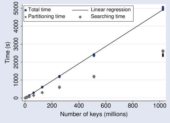
Figure 6: Partitioning time and searching time versus number of keys in $S$ for our external algorithm. The solid line corresponds to a linear regression model for the total time.

An intriguing observation is that the runtime of the algorithm is almost deterministic, in spite of the fact that it uses as building block an algorithm with a considerable fluctuation in its runtime. A given bucket $i$, $0\leq i<2^{b}$, is a small set of keys (at most 256 keys) and, the runtime of the building block algorithm is a random variable $X_{i}$ with high fluctuation (it follows a geometric distribution with mean $1/Pr\approx 3$). However, the runtime $Y$ of the searching step of our external algorithm is given by $Y=\sum_{0\leq i<2^{b}}X_{i}$. Under the hypothesis that the $X_{i}$ are independent and bounded, the law of large numbers (see, e.g., [19]) implies that the random variable $Y/2^{b}$ converges to a constant as $n\to\infty$. This explains why the runtime is almost deterministic.

The next important metric on MPHFs is the space required to store the functions. In order to apply the internal algorithm to larger sets we randomly choose $f_{0}$ and $f_{1}$ from the family of universal hash functions proposed by Thorup [33]. The internal algorithm was analyzed under the full randomness assumption so that universal hashing is not enough to guarantee that it works for every key set. But it has been the case for every key set we have applied it to. Then, we refer to this version as heuristic internal algorithm.

Table 2 shows how many bits per key the heuristic internal algorithm requires to store the resulting MPHFs. In our setup the heuristic internal algorithm requires around $2.1$ and $3.3$ bits per key to respectively store the resulting PHFs and MPHFs. In a PC with 1 gigabyte of main memory the largest set we are able to generate a MPHF for is a set with 30 millions of keys, because of the sparse graph required to generate the functions is memory demanding.

$n$	Bits/key
	PHF	MPHF
$10^{4}$	$2.13$	$3.37$
$10^{5}$	$2.09$	$3.32$
$10^{6}$	$2.09$	$3.32$
$10^{7}$	$2.09$	$3.32$

Table 2: Heuristic internal algorithm: space usage to respectively store the resulting PHFs and MPHFs.

The external algorithm is designed to be used when the key set does not fit in main memory. Table 3 shows that it can be used for constructing PHFs and MPHFs that require approximately 2.7 and 3.8 bits per key to be stored, respectively. The lookup tables used by the hash functions of the external algorithm require a fixed storage cost of 1,847,424 bytes. This makes the external algorithm unsuitable for sets with less than 16 million of keys.

$n$	$b$	Cost in bytes to	Bits/key
		store lookup tables	PHF	MPHF
$10^{4}$	6	1,847,424	$2.93$	$3.71$
$10^{5}$	9	1,847,424	$2.73$	$3.57$
$10^{6}$	13	1,847,424	$2.65$	$3.82$
$10^{7}$	16	1,847,424	$2.51$	$3.70$
$10^{8}$	20	1,847,424	$2.80$	$4.02$
$10^{9}$	23	1,847,424	$2.65$	$3.83$

Table 3: External algorithm: space usage to respectively store the resulting PHFs and MPHFs.

To overcome the problem mentioned above we have implemented a version of the external algorithm that uses the pseudo random hash function proposed by Jenkins [20]. This function was used instead of the linear hash function described in Section 4.3.2, and instead of the two truly random hash function of each bucket, i.e., $h_{i1}$ and $h_{i2}$, where $0\leq i<2^{b}$. This version is, from now on, referred to as heuristic external algorithm. The Jenkins function just loops around the key doing bitwise operations over chunks of 12 bytes. Then, it returns the last chunk. Thus, in the mapping step, the key set S is mapped to F, which now contains 12-byte long strings instead of 16-byte long strings.

The Jenkins function needs just one random seed of 32 bits to be stored instead of quite long lookup tables. Therefore, there is no fixed cost to store the resulting MPHFs, but two random seeds of 32 bits are required to describe the functions $h_{i1}$ and $h_{i2}$ of each bucket. As a consequence, the MPHFs generation and the MPHFs efficiency at retrieval time are faster (see Table 4 and 5). The reasons are twofold. First, we are dealing with 12-byte strings instead of 16-byte strings. Second, there are no large lookup tables to cause cache misses. For example, the construction time for a set of 1024 million keys has dropped down to $1.04$ hours in the same setup. The disadvantage of using the Jenkins function is that there is no formal proof that it works for every key set. That is why the hash functions we have designed in this paper are required, even being slower. In the implementation available, the hash functions to be used can be chosen by the user.

Table 4 presents a comparison of our methods with the ones proposed by Pagh [28] (Hash-displace), by Botelho, Kohayakawa and Ziviani [5] (BKZ), by Czech, Havas and Majewski [9] (CHM), and by Fox, Chen and Heath [13] (FCH), considering construction time and storage space as metrics. The form of the MPHFs generated by those methods is presented in Section 3. Notice that they are the most important practical results on MPHFs known in the literature. Observing the results, our heuristic internal algorithm is the best choice for sets that can be handled in main memory and our external algorithm is the first one that can be applied to sets that do not fit in main memory.

Time in seconds to construct a MPHF for $2\times 10^{6}$ keys
Algorithms	Function	Construction	bits/key
	type	time (seconds)
Heuristic Internal	PHF	$12.99\pm 1.01$	$2.09$
Algorithm	MPHF	$13.94\pm 1.06$	$3.35$
External	PHF	$6.92\pm 0.04$	$2.64$
Algorithm	MPHF	$6.98\pm 0.01$	$3.85$
Heuristic External	MPHF	$4.75\pm 0.02$	$3.7$
Algorithm
Hash-displace	MPHF	$46.18\pm 1.06$	$64.00$
BKZ	MPHF	$8.57\pm 0.31$	$32.00$
CHM	MPHF	$13.80\pm 0.70$	$66.88$
FCH	MPHF	$758.66\pm 126.72$	$5.84$

Table 4: Construction time and storage space without considering the fixed cost to store lookup tables.

Finally, we show how efficient is the resulting MPHFs at retrieval time for the methods aforementioned, which is as important as construction time and storage space. Table 5 presents the time, in seconds, to evaluate $2\times 10^{6}$ keys. We group the BKZ and CHM methods together because the resulting MPHFs have the same form. From the results we can conclude that our heuristic internal algorithm generates MPHFs that are as fast to be computed as the ones generated by the most practical methods on MPHFs. The MPHFs generated by the external algorithm are slower. Nevertheless, the difference is not so expressive (each key can be evaluated in few microseconds) and the external algorithm is the first efficient option for sets that do not fit in main memory.

Time in seconds to evaluate $2\times 10^{6}$ keys
key length (bytes)	Function	8	16	32	64	128
	type
Heuristic Internal	PHF	0.41	0.55	0.79	1.29	2.39
Algorithm	MPHF	0.85	0.99	1.23	1.73	2.74
External	PHF	2.05	2.31	2.84	3.99	7.22
Algorithm	MPHF	2.55	2.83	3.38	4.63	8.18
Heuristic External	MPHF	1.19	1.35	1.59	2.11	3.34
Algorithm
Hash-displace	MPHF	0.56	0.69	0.93	1.44	2.54
BKZ/CHM	MPHF	0.61	0.74	0.98	1.48	2.58
FCH	MPHF	0.58	0.72	0.96	1.46	2.56

Table 5: Evaluation time.

It is important to emphasize that the BKZ, CHM and FCH methods were analyzed under the full randomness assumption as well as our heuristic internal algorithm. Therefore, our external algorithm is the first one that has experimentally proven practicality for large key sets and has both space usage for representing the resulting functions and the construction time carefully proven. Additionally, it is the fastest algorithm for constructing the functions and the resulting functions are much simpler than the ones generated by previous theoretical well-founded schemes so that they can be used in practice. Also, it considerably improves the first step given by Pagh with his hash and displace method [28].

5.3 Controlling disk accesses

In order to bring down the number of seek operations on disk we benefit from the fact that our external algorithm leaves almost all main memory available to be used as disk I/O buffer. In this section we evaluate how much the parameter $\mu$ affects the runtime of our external algorithm. For that we fixed $n$ in approximately 1 billion of URLs, set the main memory of the machine used for the experiments to 1 gigabyte and used $\mu$ equal to 100, 200, 300, 400 and 500 megabytes.

In order to amortize the number of seeks performed we use a buffering technique [21]. We create a buffer $j$ of size ฿$\>=\mu/N$ for each file $j$, where $1\leq j\leq N$. Every time a read operation is requested to file $j$ and the data is not found in the $j$th buffer, ฿ bytes are read from file $j$ to buffer $j$. Hence, the number of seeks performed in the worst case is given by $\beta/$฿ (remember that $\beta$ is the size in bytes of the fixed-length key set $F$). For that we have made the pessimistic assumption that one seek happens every time buffer $j$ is filled in. Thus, the number of seeks performed in the worst case is $16n/$฿, since after the partitioning step we are dealing with 128-bit (16-byte) strings instead of 64-byte URLs, on average. Therefore, the number of seeks is linear on $n$ and amortized by ฿. It is important to emphasize that the operating system uses techniques to diminish the number of seeks and the average seek time. This makes the amortization factor to be greater than ฿ in practice.

Table 6 presents the number of files $N$, the buffer size used for all files, the number of seeks in the worst case considering the pessimistic assumption aforementioned, and the time to generate a (minimal)PHF for approximately 1 billion of keys as a function of the amount of internal memory available. Observing Table 6 we noticed that the time spent in the construction decreases as the value of $\mu$ increases. However, for $\mu>400$, the variation on the time is not as significant as for $\mu\leq 400$. This can be explained by the fact that the kernel 2.6 I/O scheduler of Linux has smart policies for avoiding seeks and diminishing the average seek time (see http://www.linuxjournal.com/article/6931).

$\mu$ (MB)	$100$	$200$	$300$	$400$	$500$
$N$ (files)	$245$	$99$	$63$	$46$	$36$
฿ (in KB)	$418$	$2,069$	$4,877$	$8,905$	$14,223$
$\beta$/฿	$151,768$	$30,662$	$13,008$	$7,124$	$4,461$
Time (hours)	$1.58$	$1.37$	$1.33$	$1.32$	$1.32$

Table 6: Influence of the internal memory area size ($\mu$) in our external algorithm runtime.

6 Concluding remarks

This paper has presented two novel algorithms for constructing PHFs and MPHFs and three implementations of the algorithms. The implementations in the C language are available at http://anonymous under the GNU Lesser General Public License (LGPL).

The first algorithm, referred to as internal algorithm, assumes that two truly random hash functions $f_{0}$ and $f_{1}$ are available for free so that a PHF or a MPHF can be constructed from the acyclic random graph induced by $f_{0}$ and $f_{1}$. The full randomness assumption is not realistic because each truly random hash functions would require at least $n\log n$ bits to be stored, which is memory demanding.

In order to compare the internal algorithm with the most important practical results on MPHFs that consider the same assumption (see Section 3) we have chosen the required hash functions from the family of universal hash functions proposed by Thorup [33]. As universal hash functions are not enough to guarantee that the algorithm would work for every key set, then we have referred to this version of the algorithm as heuristic internal algorithm.

The heuristic internal algorithm outperforms all previous methods considering the storage space required for the resulting functions. The resulting PHFs and MPHFs require approximately 2.1 and 3.3 bits per key to be stored, respectively. Better still, the resulting functions are almost as fast to be computed and generated as the ones coming from previous methods known in the literature. Tables 2, 4 and 5 summarize the experimental results.

The second algorithm, referred to as external algorithm, contains, as a component, a provably good implementation of the internal memory algorithm. This means that the two hash functions $h_{i1}$ and $h_{i2}$ (see Eq. (4.3.1)) used instead of $f_{0}$ and $f_{1}$ behave as truly random hash functions (see Section 4.3.3). The resulting PHFs and MPHFs require approximately 2.7 and 3.8 bits per key to be stored and are generated faster than the ones generated by all previous methods (including our heuristic internal algorithm). The external algorithm is the first one that has experimentally proven practicality for sets in the order of billions of keys and has time and space usage carefully analyzed without unrealistic assumptions. As a consequence, the external algorithm will work for every key set.

The resulting functions of the external algorithm are approximately four times slower than the ones generated by our heuristic internal algorithm and by all previous practical methods (see Table 5). The reason is that to compute the involved hash functions we need to access lookup tables that do not fit in the cache. To overcome this problem, at the expense of losing the guarantee that it works for every key set, we have proposed a heuristic version of the external algorithm that uses a very efficient pseudo random hash function proposed by Jenkins [20]. The resulting functions require the same storage space, are now less than two times slower to be computed and are still faster to be generated.

Besides the data management applications for minimal perfect hash functions described in Section 1, the external algorithm will be very useful for the information retrieval community as well. Search engines are nowadays indexing tens of billions of pages and the work with huge collections is becoming a daily task. For instance, the simple assignment of number identifiers to web pages of a collection can be a challenging task. While traditional databases simply cannot handle more traffic once the working set of URLs does not fit in main memory anymore [32], the external algorithm we propose here to construct MPHFs can easily scale to billions of entries. Also, algorithms like PageRank [6], which uses the web link structure to derive a measure of popularity for Web pages, operates on the web graph. At construction time of the graph, the URLs must be mapped to integers that will be used to label the vertices. For the same reason, the WebGraph research group [3] would also benefit from a MPHF for sets in the order of billions of URLs to scale and to improve the storage requirements of their algorithms on Graph compression.

References

- [1] N. Alon, M. Dietzfelbinger, P. B. Miltersen, E. Petrank, and G. Tardos. Linear hash functions. Journal of the ACM, 46(5):667–683, 1999.
- [2] N. Alon and M. Naor. Derandomization, witnesses for Boolean matrix multiplication and construction of perfect hash functions. Algorithmica, 16(4-5):434–449, 1996.
- [3] P. Boldi and S. Vigna. The webgraph framework i: Compression techniques. In Proceedings of the 13th International World Wide Web Conference (WWW’04), pages 595–602, 2004.
- [4] B. Bollobás. Random graphs, volume 73 of Cambridge Studies in Advanced Mathematics. Cambridge University Press, Cambridge, second edition, 2001.
- [5] F. Botelho, Y. Kohayakawa, and N. Ziviani. A practical minimal perfect hashing method. In Proceedings of the 4th International Workshop on Efficient and Experimental Algorithms (WEA’05), pages 488–500. Springer Lecture Notes in Computer Science vol. 3503, 2005.
- [6] S. Brin and L. Page. The anatomy of a large-scale hypertextual web search engine. In Proceedings of the 7th International World Wide Web Conference (WWW’98), pages 107–117, April 1998.
- [7] C.-C. Chang and C.-Y. Lin. A perfect hashing schemes for mining association rules. The Computer Journal, 48(2):168–179, 2005.
- [8] C.-C. Chang, C.-Y. Lin, and H. Chou. Perfect hashing schemes for mining traversal patterns. Journal of Fundamenta Informaticae, 70(3):185–202, 2006.
- [9] Z. Czech, G. Havas, and B. Majewski. An optimal algorithm for generating minimal perfect hash functions. Information Processing Letters, 43(5):257–264, 1992.
- [10] Z. Czech, G. Havas, and B. Majewski. Fundamental study perfect hashing. Theoretical Computer Science, 182:1–143, 1997.
- [11] E. Demaine, F. M. auf der Heide, R. Pagh, and M. Pǎtraşcu. De dictionariis dynamicis pauco spatio utentibus. In Proceedings of the Latin American Symposium on Theoretical Informatics (LATIN’06), pages 349–361, 2006.
- [12] M. Dietzfelbinger and T. Hagerup. Simple minimal perfect hashing in less space. In Proceedings of the 9th European Symposium on Algorithms (ESA’01), pages 109–120. Springer Lecture Notes in Computer Science vol. 2161, 2001.
- [13] E. Fox, Q. Chen, and L. Heath. A faster algorithm for constructing minimal perfect hash functions. In Proceedings of the 15th Annual International ACM SIGIR Conference on Research and Development in Information Retrieval, pages 266–273, 1992.
- [14] E. Fox, L. S. Heath, Q. Chen, and A. Daoud. Practical minimal perfect hash functions for large databases. Communications of the ACM, 35(1):105–121, 1992.
- [15] M. L. Fredman, J. Komlós, and E. Szemerédi. On the size of separating systems and families of perfect hashing functions. SIAM Journal on Algebraic and Discrete Methods, 5:61–68, 1984.
- [16] M. L. Fredman, J. Komlós, and E. Szemerédi. Storing a sparse table with O(1) worst case access time. Journal of the ACM, 31(3):538–544, July 1984.
- [17] T. Hagerup and T. Tholey. Efficient minimal perfect hashing in nearly minimal space. In Proceedings of the 18th Symposium on Theoretical Aspects of Computer Science (STACS’01), pages 317–326. Springer Lecture Notes in Computer Science vol. 2010, 2001.
- [18] G. Havas, B. Majewski, N. Wormald, and Z. Czech. Graphs, hypergraphs and hashing. In Proceedings of the 19th International Workshop on Graph-Theoretic Concepts in Computer Science, pages 153–165. Springer Lecture Notes in Computer Science vol. 790, 1993.
- [19] R. Jain. The art of computer systems performance analysis: techniques for experimental design, measurement, simulation, and modeling. John Wiley, first edition, 1991.
- [20] B. Jenkins. Algorithm alley: Hash functions. Dr. Dobb’s Journal of Software Tools, 22(9), september 1997.
- [21] D. E. Knuth. The Art of Computer Programming: Sorting and Searching, volume 3. Addison-Wesley, second edition, 1973.
- [22] P. Larson and G. Graefe. Memory management during run generation in external sorting. In Proceedings of the 1998 ACM SIGMOD international conference on Management of data, pages 472–483. ACM Press, 1998.
- [23] S. Lefebvre and H. Hoppe. Perfect spatial hashing. ACM Transactions on Graphics, 25(3):579–588, 2006.
- [24] B. Majewski, N. Wormald, G. Havas, and Z. Czech. A family of perfect hashing methods. The Computer Journal, 39(6):547–554, 1996.
- [25] S. Manegold, P. A. Boncz, and M. L. Kersten. Optimizing database architecture for the new bottleneck: Memory access. The VLDB journal, 9:231–246, 2000.
- [26] K. Mehlhorn. Data Structures and Algorithms 1: Sorting and Searching. Springer-Verlag, 1984.
- [27] A. Pagh, R. Pagh, and S. S. Rao. An optimal bloom filter replacement. In Proceedings of the 16th annual ACM-SIAM symposium on Discrete algorithms (SODA’05), pages 823–829, Philadelphia, PA, USA, 2005.
- [28] R. Pagh. Hash and displace: Efficient evaluation of minimal perfect hash functions. In Workshop on Algorithms and Data Structures (WADS’99), pages 49–54, 1999.
- [29] R. Pagh. Low redundancy in static dictionaries with constant query time. SIAM Journal on Computing, 31(2):353–363, 2001.
- [30] J. Radhakrishnan. Improved bounds for covering complete uniform hypergraphs. Information Processing Letters, 41:203–207, 1992.
- [31] J. P. Schmidt and A. Siegel. The spatial complexity of oblivious k-probe hash functions. SIAM Journal on Computing, 19(5):775–786, October 1990.
- [32] M. Seltzer. Beyond relational databases. ACM Queue, 3(3), April 2005.
- [33] M. Thorup. Even strongly universal hashing is pretty fast. In Proceedings of the eleventh annual ACM-SIAM symposium on Discrete algorithms (SODA’00), pages 496–497, Philadelphia, PA, USA, 2000.