Attribute Value Reordering For Efficient Hybrid OLAP

Abstract

The normalization of a data cube is the ordering of the attribute values. For large multidimensional arrays where dense and sparse chunks are stored differently, proper normalization can lead to improved storage efficiency. We show that it is NP-hard to compute an optimal normalization even for $1\times 3$ chunks, although we find an exact algorithm for $1\times 2$ chunks. When dimensions are nearly statistically independent, we show that dimension-wise attribute frequency sorting is an optimal normalization and takes time $O(dn\log(n))$ for data cubes of size $n^{d}$. When dimensions are not independent, we propose and evaluate a several heuristics. The hybrid OLAP (HOLAP) storage mechanism is already 19%–30% more efficient than ROLAP, but normalization can improve it further by 9%–13% for a total gain of 29%–44% over ROLAP.

1 Introduction

On-line Analytical Processing (OLAP) is a database acceleration technique used for deductive analysis [2]. The main objective of OLAP is to have constant-time or near constant-time answers for many typical queries. For example, in a database containing salesmen’s performance data, one may want to compute on-line the amount of sales done in Ontario for the last 10 days, including only salesmen who have 2 or more years of experience. Using a relational database containing sales information, such a computation may be expensive. Using OLAP, however, the computation is typically done on-line. To achieve such acceleration one can create a cube of data, a map from all attribute values to a given measure. In the example above, one could map tuples containing days, experience of the salesmen, and locations to the corresponding amount of sales.

We distinguish two types of OLAP engines: Relational OLAP (ROLAP) and Multidimensional OLAP (MOLAP). In ROLAP, the data is itself stored in a relational database whereas with MOLAP, a large multidimensional array is built with the data. In MOLAP, an important step in building a data cube is choosing a normalization, which is a mapping from attribute values to the integers used to index the array. One difficulty with MOLAP is that the array is often sparse. For example, not all tuples (day, experience, location) would match sales. Because of this sparseness, ROLAP uses far less storage. Additionally, there are compression algorithms to further decrease ROLAP storage requirements [3, 4, 5]. On the other hand, MOLAP can be much faster, especially if subsets of the data cube are dense [6]. Many vendors such as Speedware, Hyperion, IBM, and Microsoft are thus using Hybrid OLAP (HOLAP), storing dense regions of the cube using MOLAP and storing the rest using a ROLAP approach.

While various efficient heuristics exist to find dense sub-cubes in data cubes [7, 8, 9], the dense sub-cubes are normalization-dependent. A related problem with MOLAP or HOLAP is that the attribute values may not have a canonical ordering, so that the exact representation chosen for the cube is arbitrary. In the salesmen example, imagine that “location” can have the values “Ottawa,” “Toronto,” “Montreal,” “Halifax,” and “Vancouver.” How do we order these cities: by population, by latitude, by longitude, or alphabetically? Consider the example given in Table 1: it is obvious that HOLAP performance will depend on the normalization of the data cube. A storage-efficient normalization may lead to better query performance.

Table 1: Two tables representing the volume of sales for a given day by the experience level of the salesmen. Given that three cities only have experienced salesmen, some orderings (left) will lend themselves better to efficient storage (HOLAP) than others (right).

	<1 yrs	1–2 yrs	>2 yrs
Ottawa			$732
Toronto			$643
Montreal			$450
Halifax	$43	$54
Vancouver	$76	$12

	<1 yrs	1–2 yrs	>2 yrs
Halifax	$43	$54
Montreal			$450
Ottawa			$732
Vancouver	$76	$12
Toronto			$643

One may object that normalization only applies when attribute values are not regularly sampled numbers. One argument against normalization of numerical attribute values is that storing an index map from these values to the actual index in the cube amounts to extra storage. This extra storage is not important. Indeed, consider a data cube with $n$ attribute values per dimension and $d$ dimensions: we say such a cube is regular or $n$-regular. The most naive way to store such a map is for each possible attribute value to store a new index as an integer from $1$ to $n$. Assuming that indices are stored using $\log n$ bits, this means that $n\log n$ bits are required. However, array-based storage of a regular data cube uses $\Theta(n^{d})$ bits. In other words, unless $d=1$, normalization is not a noticeable burden and all dimensions can be normalized.

Normalization may degrade performance if attribute values often used together are stored in physically different areas thus requiring extra IO operations. When attribute values have hierarchies, it might even be desirable to restrict the possible reorderings. However, in itself, changing the normalization does not degrade the performance of a data cube, unlike many compression algorithms. While automatically finding the optimal normalization may be difficult when first building the data cube, the system can run an optimization routine after the data cube has been built, possibly as a background task.

1.1 Contributions and Organization

The contributions of this paper include a detailed look at the mathematical foundations of normalization, including notation for the remainder of the paper and future work on normalization of block-coded data cubes (Sections 2 and 3). In particular, Section 3 includes a theorem showing that determining whether two data cubes are equivalent for the normalization problem is Graph Isomorphism-complete. Section 4 considers the computational complexity of normalization. If data cubes are stored in tiny (size-2) blocks, an exact algorithm can compute the best normalization, whereas for larger blocks, it is conjectured that the problem is NP-hard. As evidence, we show that the case of size-3 blocks is NP-hard. Establishing that even trivial cases are NP-hard helps justify use of heuristics. Moreover, the optimal algorithm used for tiny blocks leads us to the Iterated Matching (IM) heuristic presented later. An important class of “slice-sorting” normalizations is investigated in Section 5. Using a notion of statistical independence, a major contribution (Theorem 18) is an easily computed approximation bound for a heuristic called “Frequency Sort,” which we show to be the best choice among our heuristics when the cube dimensions are nearly statistically independent. Section 6 discusses additional heuristics that could be used when the dimensions of the cube are not sufficiently independent. In Section 7, experimental results compare the performance of heuristics on a variety of synthetic and “real-world” data sets. The paper concludes with Section 8. A glossary is provided at the end of the paper.

2 Block-Coded Data Cubes

In what follows, $d$ is the number of dimensions (or attributes) of the data cube $C$ and $n_{i}\mbox{, for\ }1\leq i\leq d$, is the number of attribute values for dimension $i$. Thus, $C$ has size $n_{1}\times\ldots\times n_{d}$. To be precise, we distinguish between the cells and the indices of a data cube. “Cell” is a logical concept and each cell corresponds uniquely to a combination of values $(v_{1},v_{2},\ldots,v_{d})$, with one value $v_{i}$ for each attribute $i$. In Table 1, one of the 15 cells corresponds to (Montreal, 1–2 yrs). Allocated cells, such as (Vancouver, 1–2 yrs), store measure values, in contrast to unallocated cells such as (Montreal, 1–2 yrs). From now on, we shall assume that some initial normalization has been applied to the cube and that attribute $i$’s values are $\{1,2,\ldots n_{i}\}$. “Index” is a physical concept and each $d$-tuple of indices specifies a storage location within a cube. At this location there is a cell, allocated or otherwise. (Re-) normalization changes neither the cells nor the indices of the cube; (Re-)normalization changes the assignment of cells to indices.

We use $\#C$ to denote the number of allocated cells in cube $C$. Furthermore, we say that $C$ has density $\rho=\frac{\#C}{n_{1}\times\ldots\times n_{d}}$. While we can optimize storage requirements and speed up queries by providing approximate answers [10, 11, 12], we focus on exact methods in this paper, and so we seek an efficient storage mechanism to store all $\#C$ allocated cells.

There are many ways to store data cubes using different coding for dense regions than for sparse ones. For example, in one paper [9] a single dense sub-cube (chunk) with $d$ dimensions is found and the remainder is considered sparse.

We follow earlier work [2, 13] and store the data cube in blocks, which are disjoint $d$-dimensional sub-cubes covering the entire data cube. We consider blocks of constant size $m_{1}\times\ldots\times m_{d}$; thus, there are $\lceil\frac{n_{1}}{m_{1}}\rceil\times\ldots\times\lceil\frac{n_{d}}{m_{d}}\rceil$ blocks. For simplicity, we usually assume that $m_{k}$ divides $n_{k}$ for all $k\in\{1,\ldots,d\}$. Each block can then be stored in an optimized way depending, for example, on its density. We consider only two widely used coding schemes for data cubes, corresponding respectively to simple ROLAP and simple MOLAP. That is, either we represent the block as a list of tuples, one for each allocated cell in the block, or else we code the block as an array. For both extreme cases, a very dense or a very sparse block, MOLAP and ROLAP are respectively efficient. More aggressive compression is possible [14], but as long as we use block-based storage, normalization is a factor.

Assuming that a data cube is stored using block encoding, we need to estimate the storage cost. A simplistic model is given as follows. The cost of storing a single cell sparsely, as a tuple containing the position of the value in the block as $d$ attribute values (cost proportional to $d$) and the measure value itself (cost of 1), is assumed to be $1+\alpha d$, where parameter $\alpha$ can be adjusted to account for size differences between measure values and attribute values. Setting $\alpha$ small would favor sparse encoding (ROLAP) whereas setting $\alpha$ large would favor dense encoding (MOLAP). For example, while we might store 32-bit measure values, the number of values per attribute in a given block is likely less than $2^{16}$. This motivates setting $\alpha=1/2$ in later experiments and the remainder of the section. Thus, densely storing a block with $D$ allocated cells costs $M=m_{1}\times\ldots\times m_{d}$, but storing it sparsely costs $(d/2+1)D$.

It is more economical to store a block densely if $(d/2+1)D>M$, that is, if $\frac{D}{m_{1}\times\ldots\times m_{d}}>\frac{1}{d/2+1}$. This block coding is least efficient when a data cube has uniform density $\rho$ over all blocks. In such cases, it has a sparse storage cost of $d/2+1$ per allocated cell if $\rho\leq\frac{1}{d/2+1}$ or a dense storage cost of $1/\rho$ per allocated cell if $\rho>\frac{1}{d/2+1}$. Given a data cube $C$, $H(C)$ denotes its storage cost. We have $\#C\leq H(C)\leq n_{1}\times\ldots\times n_{d}$. Thus, we measure the cost per allocated cell $E(C)$ as $\frac{H(C)}{\#C}$ with the convention that if $\#C=0$, then $E(C)=1$. The cost per allocated cell is bounded by 1 and $d/2+1$: $1\leq E(C)\leq d/2+1$. A weakness of the model is that it ignores obvious storage overheads proportional to the number of blocks, $\frac{n_{1}}{m_{1}}\times\ldots\times\frac{n_{d}}{m_{d}}$. However, as long as the number of blocks remains constant, it is reasonable to assume that the overhead is constant. Such is the case when we consider the same data cube under different normalizations using fixed block dimensions.

3 Mathematical Preliminaries

Now that we have defined a simple HOLAP model, we review two of the most important concepts in this paper: slices and normalizations. Whereas a slice amounts to fixing one of the attributes, a normalization can be viewed as a tuple of permutations.

3.1 Slices

Figure 1: A $3\times 3\times 3$ cube $C$ with the slice $C^{1}_{3}$ shaded.

Consider an $n$-regular $d$-dimensional cube $C$ and let $C_{i_{1},\ldots,i_{d}}$ denote the cell stored at indices $(i_{1},\ldots,i_{d})\in\left\{1,\ldots,n\right\}^{d}$. Thus, $C$ has size $n^{d}$. The slice $C_{v}^{j}$ of $C$, for index $v$ of dimension $j$ ($1\leq j\leq d$ and $1\leq v\leq n$) is a $d-1$ - dimensional cube formed as ${C_{v}^{j}}_{i_{1},\ldots,i_{j-1},i_{j+1},\ldots,i_{d}}=C_{i_{1},\ldots,i_{j-1},v,i_{j+1},\ldots,i_{d}}$ (See Figure 1).

For the normalization task, we simply need know which indices contain allocated cells. Hence we often view a slice as a $d-1$ - dimensional Boolean array $\widehat{C}_{v}^{j}$. For example, in Figure 1, we might write (linearly) $C^{1}_{3}=[0,1,0,5,9,2,4,0,0]$ and $\widehat{C}^{1}_{3}=[0,1,0,1,1,1,1,0,0]$, if we represent non-allocated cells by zeros. Let $\#\widehat{C}_{v}^{j}$ denote the number of allocated cells in slice $C_{v}^{j}$.

3.2 Normalizations and Permutations

Given a list of $n$ items, there are $n!$ distinct possible permutations noted $\Gamma_{n}$ (the Symmetry Group). If $\gamma\in\Gamma_{n}$ permutes $i$ to $j$, we write $\gamma(i)=j$. The identity permutation is denoted $\iota$. In contrast to previous work on database compression (e.g., [4]), with our HOLAP model there is no performance advantage from permuting the order of the dimensions themselves. (Blocking treats all dimensions symmetrically.) Instead, we focus on normalizations, which affect the order of each attribute’s values. A normalization $\pi$ of a data cube $C$ is a $d$-tuple $(\gamma_{1},\ldots,\gamma_{d})$ of permutations where $\gamma_{i}\in\Gamma_{n}$ for $i=1,\ldots,d$, and the normalized data cube $\pi(C)$ is $\pi(C)_{i_{1},\ldots,i_{d}}=C_{\gamma_{1}(i_{1}),\ldots,\gamma_{d}(i_{d})}$ for all $(i_{1},\ldots,i_{d})\in\left\{1,\ldots,n\right\}^{d}$. Recall that permutations, and thus normalizations, are not commutative. However, normalizations are always invertible, and there are $(n!)^{d}$ normalizations for an $n$-regular data cube. The identity normalization is denoted $I=(\iota,\ldots,\iota)$; whether $I$ denotes the identity normalization or the identity matrix will be clear from the context. Similarly $0$ may denote the zero matrix.

Given a data cube $C$, we define its corresponding allocation cube $A$ as a cube with the same dimensions, containing 0’s and 1’s depending on whether or not the cell is allocated. Two data cubes $C$ and $C^{\prime}$, and their corresponding allocation cubes $A$ and $A^{\prime}$, are equivalent ($C\sim C^{\prime}$) if there is a normalization $\pi$ such that $\pi(A)=A^{\prime}$.

The cardinality of an equivalence class is the number of distinct data cubes $C$ in this class. The maximum cardinality is $(n!)^{d}$ and there are such equivalence classes: consider the equivalence class generated by a “triangular” data cube $C_{i_{1},\ldots,i_{d}}=1$ if $i_{1}\leq i_{2}\leq\ldots\leq i_{d}$ and $0$ otherwise. Indeed, suppose that $C_{\gamma_{1}(i_{1}),\ldots,\gamma_{d}(i_{d})}=C_{\gamma^{\prime}_{1}(i_{1}),\ldots,\gamma^{\prime}_{d}(i_{d})}$ for all $i_{1},\ldots,i_{d}$, then $\gamma_{1}(i_{1})\leq\gamma_{2}(i_{2})\leq\ldots\leq\gamma_{d}(i_{d})$ if and only if $\gamma^{\prime}_{1}(i_{1})\leq\gamma^{\prime}_{2}(i_{2})\leq\ldots\leq\gamma^{\prime}_{d}(i_{d})$ which implies that $\gamma_{i}=\gamma^{\prime}_{i}$ for $i\in\{1,\ldots,d\}$. To see this, consider the 2-d case where $\gamma_{1}(i_{1})\leq\gamma_{2}(i_{2})$ if and only if $\gamma^{\prime}_{1}(i_{1})\leq\gamma^{\prime}_{2}(i_{2})$. In this case the result follows from the following technical proposition. For more than two dimensions, the proposition can be applied to any pair of dimensions.

Proposition 1

Consider any $\gamma_{1},\gamma_{2},\gamma^{\prime}_{1},\gamma^{\prime}_{2}\in\Gamma_{n}$ satisfying $\gamma_{1}(i)\leq\gamma_{2}(j)\Leftrightarrow\gamma^{\prime}_{1}(i)\leq\gamma^{\prime}_{2}(j)$ for all $1\leq i,j\leq n$. Then $\gamma_{1}=\gamma^{\prime}_{1}$ and $\gamma_{2}=\gamma^{\prime}_{2}$.

[Proof.] Fix $i$, then let $k$ be the number of $j$ values such that $\gamma_{2}(j)\geq\gamma_{1}(i)$. We have that $\gamma_{1}(i)=n-k+1$ because it is the only element of $\{1,\ldots,n\}$ having exactly $k$ values larger or equal to it. Because $\gamma_{1}(i)\leq\gamma_{2}(j)\Leftrightarrow\gamma^{\prime}_{1}(i)\leq\gamma^{\prime}_{2}(j)$, $\gamma^{\prime}_{1}(i)=n-k+1$ and hence $\gamma^{\prime}_{1}=\gamma_{1}$. Similarly, fix $j$ and count $i$ values to prove that $\gamma^{\prime}_{2}=\gamma_{2}$. ∎

However, there are singleton equivalence classes, since some cubes are invariant under normalization: consider a null data cube $C_{i_{1},\ldots,i_{d}}=0$ for all $(i_{1},\ldots,i_{d})\in\left\{1,\ldots,n\right\}^{d}$.

To count the cardinality of a class of data cubes, it suffices to know how many slices $C_{v}^{j}$ of data cube $C$ are identical, so that we can take into account the invariance under permutations. Considering all $n$ slices in dimension $r$, we can count the number of distinct slices $d_{r}$ and number of copies $n_{r,1},\ldots,n_{r,d_{r}}$ of each. Then, the number of distinct permutations in dimension $r$ is $\frac{n!}{n_{r,1}!\times\ldots,\times n_{r,d_{r}}!}$ and the cardinality of a given equivalence class is $\prod_{r=1}^{d}\left(\frac{n!}{n_{r,1}!\times\ldots,\times n_{r,d_{r}}!}\right).$ For example, the equivalence class generated by $C=\begin{bmatrix}0&1\\ 0&1\end{bmatrix}$ has a cardinality of 2, despite having 4 possible normalizations.

To study the computational complexity of determining cube similarity, we define two decision problems. The problem Cube Similarity has $C$ and $C^{\prime}$ as input and asks whether $C\sim C^{\prime}$. Problem Cube Similarity (2-d) restricts $C$ and $C^{\prime}$ to two-dimensional cubes. Intuitively, Cube Similarity asks whether two data cubes offer the same problem from a normalization-efficiency viewpoint. The next theorem concerns the computational complexity of Cube Similarity (2-d), but we need the following lemma first. Recall that $(\gamma_{1},\gamma_{2})$ is the normalization with the permutation $\gamma_{1}$ along dimension 1 and $\gamma_{2}$ along dimension 2 whereas $(\gamma_{1},\gamma_{2})(I)$ is the renormalized cube.

Lemma 2

Consider the $n\times n$ matrix $I^{\prime}=(\gamma_{1},\gamma_{2})(I)$. Then $I^{\prime}=I\iff\gamma_{1}=\gamma_{2}$.

We can now state Theorem 3, which shows that determining cube similarity is Graph Isomorphism-complete [15]. A problem $\Pi$ belongs to this complexity class when both

• $\Pi$ has a polynomial-time reduction to Graph Isomorphism, and

• Graph Isomorphism has a polynomial-time reduction to $\Pi$.

Graph Isomorphism-complete problems are unlikely to be NP-complete [16], yet there is no known polynomial-time algorithm for any problem in the class. This complexity class has been extensively studied.

Theorem 3

Cube Similarity (2-d) is Graph Isomorphism-complete.

[Proof.] It is enough to consider two-dimensional allocation cubes as 0-1 matrices. The connection to graphs comes via adjacency matrices.

To show that Cube Similarity (2-d) is graph isomorphism-complete, we show two polynomial-time many-to-one reductions: the first transforms an instance of Graph Isomorphism to an instance of Cube Similarity (2-d).

The second reduction transforms an instance of Cube Similarity (2-d) to an instance of Graph Isomorphism.

The graph-isomorphism problem is equivalent to a re-normalization problem of the adjacency matrices. Indeed, consider two graphs $G_{1}$ and $G_{2}$ and their adjacency matrices $M_{1}$ and $M_{2}$. The two graphs are isomorphic if and only if there is a permutation $\gamma$ so that $(\gamma,\gamma)(M_{1})=M_{2}$. We can assume without loss of generality that all rows and columns of the adjacency matrices have at least one non-zero value, since we can count and remove disconnected vertices in time proportional to the size of the graph.

We have to show that the problem of deciding whether $\gamma$ satisfies $(\gamma,\gamma)(M_{1})=M_{2}$ can be rewritten as a data cube equivalence problem. It turns out to be possible by extending the matrices $M_{1}$ and $M_{2}$. Let $I$ be the identity matrix, and consider two allocation cubes (matrices) $A_{1}$ and $A_{2}$ and their extensions $\hat{A}_{1}=\begin{bmatrix}A_{1}&I&I\\ I&I&0\\ I&0&0\end{bmatrix}$ and $\hat{A}_{2}=\begin{bmatrix}A_{2}&I&I\\ I&I&0\\ I&0&0\end{bmatrix}.$

Consider a normalization $\pi$ satisfying $\pi(\hat{A}_{1})=\hat{A}_{2}$ for matrices $A_{1},A_{2}$ having at least one non-zero value for each column and each row. We claim that such a $\pi$ must be of the form $\pi=(\gamma_{1},\gamma_{2})$ where $\gamma_{1}=\gamma_{2}$. By the number of non-zero values in each row and column, we see that rows cannot be permuted across the three blocks of rows because the first one has at least 3 allocated values, the second one exactly 2 and the last one exactly 1. The same reasoning applies to columns. In other words, if $x\in[j,jn]$, then $\gamma_{i}(x)\in[j,jn]$ for $j=1,2,3$ and $i=1,2$.

Let $\gamma_{i}|j$ denote the permutation $\gamma$ restricted to block $j$ where $j=1,2,3$. Define $\gamma^{j}_{i}=\gamma_{i}|j-jn$ for $j=1,2,3$ and $i=1,2$. By Lemma 2, each sub-block consisting of an identity leads to an equality between two permutations. From the two identity matrices in the top sub-blocks, for example, we have that $\gamma^{1}_{1}=\gamma^{2}_{2}$ and $\gamma^{1}_{1}=\gamma^{3}_{2}$. From the middle sub-blocks, we have $\gamma^{2}_{1}=\gamma^{1}_{2}$ and $\gamma^{2}_{1}=\gamma^{2}_{2}$, and from the bottom sub-blocks, we have $\gamma^{3}_{1}=\gamma^{1}_{2}$. From this, we can deduce that $\gamma^{1}_{1}=\gamma^{2}_{2}=\gamma^{2}_{1}=\gamma^{1}_{2}$ so that $\gamma^{1}_{1}=\gamma^{1}_{2}$ and similarly, $\gamma^{2}_{1}=\gamma^{2}_{2}$ and $\gamma^{3}_{1}=\gamma^{3}_{2}$ so that $\gamma_{1}=\gamma_{2}$.

So, if we set $A_{1}=M_{1}$ and $A_{2}=M_{2}$, we have that $G_{1}$ and $G_{2}$ are isomorphic if and only if $\hat{A}_{1}$ is similar to $\hat{A}_{2}$. This completes the proof that if the extended adjacency matrices are seen to be equivalent as allocation cubes, then the graphs are isomorphic. Therefore, we have shown a polynomial-time transformation from Graph Isomorphism to Cube Similarity (2-d).

Next, we show a polynomial-time transformation from Cube Similarity (2-d) to Graph Isomorphism. We reduce Cube Similarity (2-d) to Directed Graph Isomorphism, which is in turn reducible to Graph Isomorphism [17, 18].

Given two 0-1 matrices $M_{1}$ and $M_{2}$, we want to decide whether we can find $(\gamma_{1},\gamma_{2})$ such that $(\gamma_{1},\gamma_{2})(M_{1})=M_{2}$. We can assume that $M_{1}$ and $M_{2}$ are square matrices and if not, pad with as many rows or columns filled with zeros as needed. We want a reduction from this problem to Directed Graph Isomorphism. Consider the following matrices: $\hat{M}_{1}=\begin{bmatrix}0&M_{1}\\ 0&0\end{bmatrix}$ and $\hat{M}_{2}=\begin{bmatrix}0&M_{2}\\ 0&0\end{bmatrix}$. Both $\hat{M}_{1}$ and $\hat{M}_{2}$ can be considered as the adjacency matrices of directed graphs $G_{1}$ and $G_{2}$. Suppose that the graphs are found to be isomorphic, then there is a permutation $\gamma$ such that $(\gamma,\gamma)(\hat{M}_{1})=\hat{M}_{2}$. We can assume without loss of generality that $\gamma$ does not permute rows or columns having only zeros across halves of the adjacency matrices. On the other hand, rows containing non-zero components cannot be permuted across halves. Thus, we can decompose $\gamma$ into two disjoint permutations $\gamma^{1}$ and $\gamma^{2}$ and hence $(\gamma^{1},\gamma^{2})(M_{1})=M_{2},$ which implies $M_{1}\sim M_{2}$. On the other hand, if $M_{1}\sim M_{2}$, then there is $(\gamma^{1},\gamma^{2})$ such that $(\gamma^{1},\gamma^{2})(M_{1})=M_{2}$ and we can choose $\gamma$ as the direct sum of $\gamma^{1}$ and $\gamma^{2}$. Therefore, we have found a reduction from Cube Similarity (2-d) to Directed Graph Isomorphism and, by transitivity, to Graph Isomorphism.

Thus, Graph Isomorphism and Cube Similarity (2-d) are mutually reducible and hence Cube Similarity (2-d) is Graph Isomorphism-complete. ∎

Remark 4

If similarity between two $n\times n$ cubes can be decided in time $cn^{k}$ for some positive integers $c$ and $k\geq 2$, then graph isomorphism can be decided in O($n^{k}$) time.

Since Graph Isomorphism has been reduced to a special case of Cube Similarity, then the general problem is at least as difficult as Graph Isomorphism. Yet we have seen no reason to believe the general problem is harder (for instance, NP-complete). We suspect that a stronger result may be possible; establishing (or disproving) the following conjecture is left as an open problem.

Conjecture 5

The general Cube Similarity problem is also Graph Isomorphism-complete.

4 Computational Complexity of Optimal Normalization

It appears that it is computationally intractable to find a “best” normalization $\pi$ (i.e., $\pi$ minimizes cost per allocated cell $E(\pi(C))$) given a cube $C$ and given the blocks’ dimensions. Yet, when suitable restrictions are imposed, a best normalization can be computed (or approximated) in polynomial time. This section focuses on the effect of block size on intractability.

4.1 Tractable Special Cases

Our problem can be solved in polynomial time, if severe restrictions are placed on the number of dimensions or on block size. For instance, it is trivial to find a best normalization in 1-d. Another trivial case arises when blocks are of size 1, since then normalization does not affect storage cost. Thus, any normalization is a “best normalization.” The situation is more interesting for blocks of size 2; i.e., which have $m_{i}=2$ for some $1\leq i\leq d$ and $m_{j}=1$ for $1\leq j\leq d$ with $i\not=j$. A best normalization can be found in polynomial time, based on weighted-matching [19] techniques described next.

4.1.1 Using Weighted Matching

Given a weighted undirected graph, the weighted matching problem asks for an edge subset of maximum or minimum total weight, such that no two edges share an endpoint. If the graph is complete, has an even number of vertices, and has only positive edge weights, then the maximum matching effectively pairs up vertices.

For our problem, normalization’s effect on dimension $k$, for some $1\leq k\leq d$, corresponds to rearranging the order of the $n_{k}$ slices $C^{k}_{v}$, where $1\leq v\leq n_{k}$. In our case, we are using a block size of 2 for dimension $k$. Therefore, once we have chosen two slices $C^{k}_{v}$ and $C^{k}_{v^{\prime}}$ to be the first pair of slices, we will have formed the first layer of blocks and have stored all allocated cells belonging to these two slices. The total storage cost of the cube is thus a sum, over all pairs of slices, of the pairing-cost of the two slices composing the pair. The order in which pairs are chosen is irrelevant: only the actual matching of slices into pairs matters. Consider Boolean vectors $\mathbf{b}=\widehat{C}^{k}_{v}$ and $\mathbf{b^{\prime}}=\widehat{C}^{k}_{v^{\prime}}$. If both $\mathbf{b}_{i}$ and $\mathbf{b^{\prime}}_{i}$ are true, then the $i^{th}$ block in the pair is completely full and costs 2 to store. Similarly, if exactly one of $\mathbf{b}_{i}$ and $\mathbf{b^{\prime}}_{i}$ is true, then the block is half-full. Under our model, a half-full block also costs 2, but an empty block costs 0. Thus, given any two slices, we can compute the cost of pairing them by summing the storage costs of all these blocks. If we identify each slice with a vertex of a complete weighted graph, it is easy to form an instance of weighted matching. (See Figure 2 for an example.) Fortunately, cubic-time algorithms exist for weighted matching [20], and $n_{k}$ is often small enough that cubic running time is not excessive. Unfortunately, calculating the $n_{k}(n_{k}-1)/2$ edge weights is expensive; each involves two large Boolean vectors with $\frac{1}{n_{k}}\prod_{i=1}^{d}n_{i}$ elements, for a total edge-calculation time of $\Theta\left(n_{k}\prod_{i=1}^{d}n_{i}\right)$. Fortunately, this can be improved for sparse cubes.

In the 2-d case, given any two rows, for example $r_{1}=\begin{bmatrix}0&0&1&1\end{bmatrix}$ and $r_{2}=\begin{bmatrix}0&1&0&1\end{bmatrix}$, then we can compute the total allocation cost of grouping the two together as $2(\#r_{1}+\#r_{2}-\mathit{benefit})$ where $\mathit{benefit}$ is the number of positions (in this case 1) where both $r_{1}$ and $r_{2}$ have allocated cells. (This benefit records that one of the two allocated values could be stored “for free,” were slices $r_{1}$ and $r_{2}$ paired.)

According to this formula, the cost of putting $r_{1}$ and $r_{2}$ together is thus $2(2+2-1)=6$. Using this formula, we can improve edge-calculation time when the cube is sparse. To do so, for each of the $n_{k}$ slices $C^{k}_{v}$, represent each allocated value by a $d$-tuple $(i_{1},i_{2},\ldots,i_{k-1},i_{k+1},\ldots,i_{d},i_{k})$ giving its coordinates within the slice and labeling it with the number of the slice to which it belongs. Then sort these $\#C$ tuples lexicographically, in O($\#C\log\#C$) time. For example, consider the following cube, where the rows have been labeled from $r_{0}$ to $r_{5}$ ( $r_{i}$ corresponds to $C^{1}_{i}$):

$$\begin{bmatrix}r_{0}&0&0&0&0\\ r_{1}&1&1&0&1\\ r_{2}&1&0&0&0\\ r_{3}&0&1&1&0\\ r_{4}&0&1&0&0\\ r_{5}&1&0&0&1\end{bmatrix}.$$

We represent the allocated cells as {$(0,r_{1})$, $(1,r_{1})$, $(3,r_{1})$, $(0,r_{2})$, $(1,r_{3})$, $(2,r_{3})$, $(1,r_{4})$, $(0,r_{5})$, and $(3,r_{5})$}. We can then sort these to get $(0,r_{1})$, $(0,r_{2})$, $(0,r_{5})$, $(1,r_{1})$, $(1,r_{3})$, $(1,r_{4})$, $(2,r_{3})$, $(3,r_{1})$, $(3,r_{5})$. This groups together allocated cells with corresponding locations but in different slices. For example, two groups are ($(0,r_{1})$, $(0,r_{2})$, $(0,r_{5})$) and ($(1,r_{1})$, $(1,r_{3})$, $(1,r_{4})$). Initialize the benefit value associated to each edge to zero, and next process each group. Let $g$ denote the number of tuples in the current group, and in $O(g^{2})$ time examine all $g\choose 2$ pairs of slices $(s_{1},s_{2})$ in the group, and increment (by 1) the benefit of the graph edge $(s_{1},s_{2})$. In our example, we would process the group ($(0,r_{1})$, $(0,r_{2})$, $(0,r_{5})$) and increment the benefits of edges ($r_{1},r_{2}$), ($r_{2},r_{5}$), and ($r_{1},r_{5}$). For group ($(1,r_{1})$, $(1,r_{3})$, $(1,r_{4})$), we would increase the benefits of edges ($r_{1},r_{3}$), ($r_{1},r_{4}$), and ($r_{3},r_{4}$). Once all $\#C$ sorted tuples have been processed, the eventual weight assigned to edge $(v,w)$ is $2(\#\hat{C}^{k}_{v}+\#\hat{C}^{k}_{w}-\mathit{benefit}(v,w))$. In our example, we have that edge $(r_{1},r_{2})$ has a benefit of 1, and so a weight of $2(\#r_{1}+\#r_{2}-\mathit{benefit})=2(3+1-1)=6$.

A crude estimate of the running time to process the groups would be that each group is O($n_{k}$) in size, and there are O($\#C$) groups, for a time of O($\#Cn^{2}_{k}$). It can be shown that time is maximized when the $\#C$ values are distributed into $\#C/n_{k}$ groups of size $n_{k}$, leading to a time bound of $\Theta(\#Cn_{k})$ for group processing, and an overall edge-calculation time of $\#C(n_{k}+\log\#C)$.

Theorem 6

The best normalization for blocks of size $\overbrace{1\times\ldots\times 1}^{i}\times 2\times\overbrace{1\ldots\times 1}^{k-1-i}$ can be computed in $O(n_{k}\times(n_{1}\times n_{2}\times\ldots\times n_{d})+n_{k}^{3})$ time.

The improved edge-weight calculation (for sparse cubes) leads to the following.

Corollary 7

The best normalization for blocks of size $\overbrace{1\times\ldots\times 1}^{i}\times 2\times\overbrace{1\ldots\times 1}^{k-1-i}$ can be computed in $O(\#C(n_{k}+\log\#C)+n_{k}^{3})$ time.

Figure 2: Mapping a normalization problem to a weighted matching problem on graphs. Rows are labeled and we try to reorder them, given block dimensions $2\times 1$ (where 2 is the vertical dimension). In this example, optimal solutions include $r_{0},r_{1},r_{2},r_{3}$ and $r_{2},r_{3},r_{1},r_{0}$.

For more general block shapes, this algorithm is no longer optimal but nevertheless provides a basis for sensible heuristics.

4.2 An NP-hard Case

In contrast to the $1\times 2$-block situation, we next show that it is NP-hard to find the best normalization for $1\times 3$ blocks. The associated decision problem asks whether any normalization can store a given cube within a given storage bound, assuming $1\times 3$ blocks. We return to the general cost model from Section 2 but choose $\alpha=1/4$, as this results in an especially simple situation where a block with three allocated cells ($D=3$) stores each of them at a cost of 1, whereas a block with fewer than three allocated cells stores each allocated cell at a cost of $3/2$.

The proof involves a reduction from the NP-complete problem Exact 3-Cover (X3C), a problem which gives a set $S$ and a set $\mathcal{T}$ of three-element subsets of $S$. The question, for X3C, is whether there is a $\mathcal{T}^{\prime}\subseteq\mathcal{T}$ such that each $s\in S$ occurs in exactly one member of $\mathcal{T}^{\prime}$ [17].

We sketch the reduction next. Given an instance of X3C, form an instance of our problem by making a $|\mathcal{T}|\times|S|$ cube. For $s\in S$ and $T\in\mathcal{T}$, the cube has an allocated cell corresponding to $(T,s)$ if and only if $s\in T$. Thus, the cube has $3|\mathcal{T}|$ cells that need to be stored. The storage cost cannot be lower than $\frac{9|\mathcal{T}|-|S|}{2}$ and this bound can be met if and only if the answer to the instance of X3C is “yes.” Indeed, a normalization for $1\times 3$ blocks can be viewed as simply grouping the values of an attribute into triples. Suppose the storage bound is achieved, then at least $|S|$ cells would have to be stored in full blocks. Consider some full block and note there are only 3 allocated cells in each row, so all 3 of them must be chosen (because blocks are $1\times 3$). But the three allocated cells in a row can be mapped to a $T\in\mathcal{T}$. Choose it for $\mathcal{T^{\prime}}$. None of these 3 cells’ columns intersect any other full blocks, because that would imply some other row had exactly the same allocation pattern and hence represents the same $T$, which it cannot. So we see that each $s\in S$ (column) must intersect exactly one full block, showing that $\mathcal{T^{\prime}}$ is the cover we seek.

Conversely, suppose $\mathcal{T^{\prime}}$ is a cover for X3C. Order the elements in $\mathcal{T^{\prime}}$ arbitrarily as $T_{0},T_{1},\ldots,T_{|S|/3}$ and use any normalization that puts first (in arbitrary order) the three $s\in T_{0}$, then next puts the three $s\in T_{1}$, and so forth. The three allocated cells for each $T_{i}$ will be together in a (full) block, giving us at least the required “space savings” of $\frac{3}{2}|\mathcal{T^{\prime}}|=|S|$.

Theorem 8

It is NP-hard to find the best normalization when $1\times 3$ blocks are used.

We conjecture that it is NP-hard to find the best normalization whenever the block size is fixed at any size larger than 2. A related 2-d problem that is NP-hard was discussed by Kaser [21]. Rather than specify the block dimensions, this problem allows the solution to specify how to divide each dimension into two ranges, thus making four blocks in total (of possibly different shape) .

5 Slice-Sorting Normalization for Quasi-Independent Attributes

In practice, whether or not a given cell is allocated may depend on the corresponding attribute values independently of each other. For example, if a store is closed on Saturdays almost all year, a slice corresponding to “weekday=Saturday” will be sparse irrespective of the other attributes. In such cases, it is sufficient to normalize the data cube using only an attribute-wise approach. Moreover, as we shall see, one can easily compute the degree of independence of the attributes and thus decide whether or not potentially more expensive algorithms need to be used.

We begin by examining one of the simplest classes of normalization algorithms, and we will assume $n$-regular data cubes for $n\geq 3$. We say that a sequence of values $x_{1},\ldots,x_{n}$ is sorted in increasing (respectively, decreasing) order if $x_{i}\leq x_{i+1}$ (respectively, $x_{i}\geq x_{i+1}$) for $i\in\{1,\ldots,n-1\}$.

Recall that $\widehat{C}_{v}^{j}$ is the Boolean array indicating whether a cell is allocated or not in slice $C_{v}^{j}$.

Algorithm 1

(Slice-Sorting Normalization) Given an $n$-regular data cube $C$, then slices have $n^{d-1}$ cells. Given a fixed function $g:\{\mathit{true},\mathit{false}\}^{n^{d-1}}\rightarrow{\sf R\rule{0.6458pt}{5.59721pt}\hskip 3.87495pt}$, then for each attribute $j$, we compute the sequence $f_{v}^{j}=g(\widehat{C}_{v}^{j})$ for all attribute values $v=1,\ldots,n$. Let $\gamma^{j}$ be a permutation such that $\gamma^{j}(f^{j})$ is sorted either in increasing or decreasing order, then a slice-sorting normalization is $(\gamma^{1},\ldots,\gamma^{d})$.

Algorithm 1 has time complexity $O(dn^{d}+dn\log n)$. We can precompute the aggregated values $f_{v}^{j}$ and speed up normalization to $O(dn\log(n))$. It does not produce a unique solution given a function $g$ because there could be many different valid ways to sort. A normalization $\varpi=(\gamma^{1},\ldots,\gamma^{d})$ is a solution to the slice-sorting problem if it provides a valid sort for the slice-sorting problem stated by Algorithm 1 . Given a data cube $C$, denote the set of all solutions to the slice-sorting problem by $\mathcal{S}_{C,g}$. Two functions $g_{1}$ and $g_{2}$ are equivalent with respect to the slice-sorting problem if $\mathcal{S}_{C,g_{1}}=\mathcal{S}_{C,g_{2}}$ for all cubes $C$ and we write $g_{1}\simeq g_{2}$ . We can characterize such equivalence classes using monotone functions. Recall that a function $h:{\sf R\rule{0.6458pt}{5.59721pt}\hskip 3.87495pt}\rightarrow{\sf R\rule{0.6458pt}{5.59721pt}\hskip 3.87495pt}$ is strictly monotone nondecreasing (respectively, nonincreasing) if $x<y$ implies $h(x)<h(y)$ (respectively, $h(x)>h(y)$).

An alternative definition is that $h$ is monotone if, whenever $x_{1},\ldots,x_{n}$ is a sorted list, then so is $h(x_{1}),\ldots,h(x_{n})$. This second definition can be used to prove the existence of a monotone function as the next proposition shows.

Proposition 9

For a fixed integer $n\geq 3$ and two functions $\omega_{1},\omega_{2}:D\rightarrow{\sf R\rule{0.6458pt}{5.59721pt}\hskip 3.87495pt}$ where $\mathcal{D}$ is a set with an order relation, if for all sequences $x_{1},\ldots,x_{n}\in\mathcal{D}$, $\omega_{1}(x_{1}),\ldots,\omega_{1}(x_{n})$ is sorted if and only if $\omega_{2}(x_{1}),\ldots,\omega_{2}(x_{n})$ is sorted, then there is a monotone function $h:{\sf R\rule{0.6458pt}{5.59721pt}\hskip 3.87495pt}\rightarrow{\sf R\rule{0.6458pt}{5.59721pt}\hskip 3.87495pt}$ such that $\omega_{1}=h\circ\omega_{2}$.

[Proof.] The proof is constructive. Define $h$ over the image of $\omega_{2}$ by the formula

$$h(\omega_{2}(x))=\omega_{1}(x).$$

To prove that $h$ is well defined, we have to show that whenever $\omega_{2}(x_{1})=\omega_{2}(x_{2})$ then $\omega_{1}(x_{1})=\omega_{1}(x_{2})$. Suppose that this is not the case, and without loss of generality, let $\omega_{1}(x_{1})<\omega_{1}(x_{2})$. Then there is $x_{3}\in\mathcal{D}$ such that $\omega_{1}(x_{1})\leq\omega_{1}(x_{3})\leq\omega_{1}(x_{2})$ or $\omega_{1}(x_{3})\leq\omega_{1}(x_{1})$ or $\omega_{1}(x_{2})\leq\omega_{1}(x_{3})$. In all three cases, because of the equality between $\omega_{2}(x_{1})$ and $\omega_{2}(x_{2})$, any ordering of $\omega_{2}(x_{1}),\omega_{2}(x_{2}),\omega_{2}(x_{3})$ is sorted whereas there is always one non-sorted sequence using $\omega_{1}$. There is a contradiction, proving that $h$ is well defined.

For any sequence $x_{1},x_{2},x_{3}$ such that $\omega_{2}(x_{1})<\omega_{2}(x_{2})<\omega_{2}(x_{3})$, then we must either have $\omega_{1}(x_{1})\leq\omega_{1}(x_{2})\leq\omega_{1}(x_{3})$ or $\omega_{1}(x_{1})\geq\omega_{1}(x_{2})\geq\omega_{1}(x_{3})$ by the conditions of the proposition. In other words, for $x<y<z$, we either have $h(x)\leq h(y)\leq h(z)$ or $h(x)\geq h(y)\geq h(z)$ thus showing that $h$ must be monotone. ∎

Proposition 10

Given two functions $g_{1},g_{2}:\{\mathit{true},\mathit{false}\}^{S}\rightarrow{\sf R\rule{0.6458pt}{5.59721pt}\hskip 3.87495pt}$, we have that

$$\mathcal{S}_{C,g_{1}}=\mathcal{S}_{C,g_{2}}$$

for all data cubes $C$ if and only if there exist a monotone function $h:{\sf R\rule{0.6458pt}{5.59721pt}\hskip 3.87495pt}\rightarrow{\sf R\rule{0.6458pt}{5.59721pt}\hskip 3.87495pt}$ such that $g_{1}=h\circ g_{2}$.

[Proof.] Assume there is $h$ such that $g_{1}=h\circ g_{2}$, and consider $\varpi=(\gamma^{1},\ldots,\gamma^{d})\in\mathcal{S}_{C,g_{1}}$ for any data cube $C$, then $\gamma^{j}(g_{1}(\widehat{C}_{v}^{j}))$ is sorted over index $v\in\{1,\ldots,n\}$ for all attributes $j=1,\ldots,n$ by definition of $\mathcal{S}_{C,g_{1}}$. Then $\gamma^{j}(h(g_{1}(\widehat{C}_{v}^{j})))$ must also be sorted over $v$ for all $j$, since monotone functions preserve sorting. Thus $\varpi\in\mathcal{S}_{C,g_{2}}$.

One the other hand, if $\mathcal{S}_{C,g_{1}}=\mathcal{S}_{C,g_{2}}$ for all data cubes $C$, then $h$ exists by Proposition 9. ∎

A slice-sorting algorithm is stable if the normalization of a normalized cube can be chosen to be the identity, that is if $\varpi\in\mathcal{S}_{C,g}$ then $I\in\mathcal{S}_{\varpi(C),g}$ for all $C$. The algorithm is strongly stable if for any normalization $\varpi$, $\mathcal{S}_{\varpi(C),g}\circ\varpi=\mathcal{S}_{C,g}$ for all $C$. Strong stability means that the resulting normalization does not depend on the initial normalization. This is a desirable property because data cubes are often normalized arbitrarily at construction time. Notice that strong stability implies stability: choose $\varpi\in\mathcal{S}_{C,g}$. Then there must exist $\zeta\in\mathcal{S}_{\varpi(C),g}$ such that $\zeta\circ\varpi=\varpi$ which implies that $\zeta$ is the identity.

Proposition 11

Stability implies strong stability for slice-sorting algorithms and so, strong stability $\Leftrightarrow$ stability.

[Proof.] Consider a slice-sorting algorithm, based on $g$, that is stable. Then by definition

$$\varpi\in\mathcal{S}_{C,g}\Rightarrow I\in\mathcal{S}_{\varpi(C),g}$$ (1)

for all $C$. Observe that the converse is true as well, that is,

$$I\in\mathcal{S}_{\varpi(C),g}\Rightarrow\varpi\in\mathcal{S}_{C,g}.$$ (2)

Hence we have that $\varpi_{1}\circ\varpi\in\mathcal{S}_{C,g}$ implies that $I\in\mathcal{S}_{\varpi_{1}(\varpi(C)),g}$ by Equation 1 and so, by Equation 2, $\varpi_{1}\in\mathcal{S}_{\varpi(C),g}$. Note that given any $\varpi$, all elements of $\mathcal{S}_{C,g}$ can be written as $\varpi_{1}\circ\varpi$ because permutations are invertible. Hence, given $\varpi_{1}\circ\varpi\in\mathcal{S}_{C,g}$ we have $\varpi_{1}\in\mathcal{S}_{\varpi(C),g}$ and so $\mathcal{S}_{C,g}\subset\mathcal{S}_{\varpi(C),g}\circ\varpi$.

On the other hand, given $\varpi_{1}\circ\varpi\in\mathcal{S}_{\varpi(C),g}\circ\varpi$, we have that $\varpi_{1}\in\mathcal{S}_{\varpi(C),g}$ by cancellation, hence $I\in\mathcal{S}_{\varpi_{1}(\varpi(C)),g}$ by Equation 1, and then $\varpi_{1}\circ\varpi\in\mathcal{S}_{C,g}$ by Equation 2. Therefore, $\mathcal{S}_{\varpi(C),g}\circ\varpi\subset\mathcal{S}_{C,g}$. ∎

Define $\tau:\{\mathit{true},\mathit{false}\}^{S}\rightarrow{\sf R\rule{0.6458pt}{5.59721pt}\hskip 3.87495pt}$ as the number of $\mathit{true}$ values in the argument. In effect, $\tau$ counts the number of allocated cells: $\tau(\widehat{C}_{v}^{j})=\#\widehat{C}_{v}^{j}$ for any slice $\widehat{C}_{v}^{j}$. If the slice $\widehat{C}_{v}^{j}$ is normalized, $\tau$ remains constant: $\tau(\widehat{C}_{v}^{j})=\tau\left(\varpi\left(\widehat{C}_{v}^{j}\right)\right)$ for all normalizations $\varpi$. Therefore $\tau$ leads to a strongly stable slice-sorting algorithm. The converse is also true if $d=2$ , that is, if the slice is one-dimensional, then if

$$h(\widehat{C}_{v}^{j})=h\left(\varpi\left(\widehat{C}_{v}^{j}\right)\right)$$

for all normalizations $\varpi$ then $h$ can only depend on the number of allocated ($\mathit{true}$) values in the slice since it fully characterizes the slice up to normalization. For the general case ($d>2$), the converse is not true since the number of allocated values is not enough to characterize the slices up to normalization. For example, one could count how many sub-slices along a chosen second attribute have no allocated value.

A function $g$ is symmetric if $g\circ\varpi\simeq g$ for all normalizations $\varpi$. The following proposition shows that up to a monotone function, strongly stable slice-sorting algorithms are characterized by symmetric functions.

Proposition 12

A slice-sorting algorithm based on a function $g$ is strongly stable if and only if for any normalization $\varpi$, there is a monotone function $h:{\sf R\rule{0.6458pt}{5.59721pt}\hskip 3.87495pt}\rightarrow{\sf R\rule{0.6458pt}{5.59721pt}\hskip 3.87495pt}$ such that

$$g\left(\varpi\left(\widehat{C}_{v}^{j}\right)\right)=h\left(g(\widehat{C}_{v}^{j})\right)$$ (3)

for all attribute values $v=1,\ldots,n$ of all attributes $j=1,\ldots,d$. In other words, it is strongly stable if and only if $g$ is symmetric.

[Proof.] By Proposition 10, Equation 3 is sufficient for strong stability. On the other hand, suppose that the slice-sorting algorithm is strongly stable and that there does not exist a strictly monotone function $h$ satisfying Equation 3, then by Proposition 9, there must be a sorted sequence $g(\widehat{C}_{v_{1}}^{j}),g(\widehat{C}_{v_{2}}^{j}),g(\widehat{C}_{v_{3}}^{j})$ such that $g\left(\varpi\left(\widehat{C}_{v_{1}}^{j}\right)\right),g\left(\varpi\left(\widehat{C}_{v_{2}}^{j}\right)\right),g\left(\varpi\left(\widehat{C}_{v_{3}}^{j}\right)\right)$ is not sorted. Because this last statement contradicts strong stability, we have that Equation 3 is necessary. ∎

Lemma 13

A slice-sorting algorithm based on a function $g$ is strongly stable if $g=h\circ\tau$ for some function $h$. For 2-d cubes, the condition is necessary.

In the above lemma, whenever $h$ is strictly monotone, then $g\simeq\tau$ and we call this class of slice-sorting algorithms Frequency Sort [9]. We will show that we can estimate a priori the efficiency of this class (see Theorem 18).

It is useful to consider a data cube as a probability distribution in the following sense: given a data cube $C$, let the joint probability distribution $\Psi$ over the same $n^{d}$ set of indices be

$$\Psi_{i_{1},\ldots,i_{n}}=\left\{\begin{array}[]{cc}1/\#C&\mbox{if~{}}C_{i_{1},\ldots,i_{n}}\neq 0\\ 0&\mbox{otherwise}\end{array}\right..$$

The underlying probabilistic model is that allocated cells are uniformly likely to be picked whereas unallocated cells are never picked. Given an attribute $j\in\{1,\ldots,d\}$, consider the number of allocated slices in slice $C_{v}^{j}$, $\#\widehat{C}_{v}^{j}$, for $v\in\{1,\ldots,n\}$: we can define a probability distribution $\varphi^{j}$ along attribute $j$ as $\varphi_{v}^{j}=\frac{\#\widehat{C}_{v}^{j}}{\#C}$. From these $\varphi^{j}$ for all $j\in\{1,\ldots,d\}$, we can define the joint independent probability distribution $\Phi$ as $\Phi_{i_{1},\ldots,i_{d}}=\prod_{j=1}^{d}\varphi_{i_{j}}^{j},$ or in other words $\Phi=\varphi^{0}\otimes\ldots\otimes\varphi^{d-1}$. Examples are given in Table 2.

Table 2: Examples of 2-d data cubes and their probability distributions.

Data Cube	Joint Prob. Dist.	Joint Independent Prob. Dist.
$\begin{matrix}1&0&1&0\\ 0&1&0&1\\ 1&0&1&0\\ 0&1&0&1\end{matrix}$	$\begin{matrix}\frac{1}{8}&0&\frac{1}{8}&0\\ 0&\frac{1}{8}&0&\frac{1}{8}\\ \frac{1}{8}&0&\frac{1}{8}&0\\ 0&\frac{1}{8}&0&\frac{1}{8}\end{matrix}$	$\begin{matrix}\frac{1}{16}&\frac{1}{16}&\frac{1}{16}&\frac{1}{16}\\ \frac{1}{16}&\frac{1}{16}&\frac{1}{16}&\frac{1}{16}\\ \frac{1}{16}&\frac{1}{16}&\frac{1}{16}&\frac{1}{16}\\ \frac{1}{16}&\frac{1}{16}&\frac{1}{16}&\frac{1}{16}\end{matrix}$
$\begin{matrix}1&0&0&0\\ 0&1&0&0\\ 0&1&1&0\\ 0&0&0&0\end{matrix}$	$\begin{matrix}\frac{1}{4}&0&0&0\\ 0&\frac{1}{4}&0&0\\ 0&\frac{1}{4}&\frac{1}{4}&0\\ 0&0&0&0\end{matrix}$	$\begin{matrix}\frac{1}{16}&\frac{1}{8}&\frac{1}{16}&0\\ \frac{1}{16}&\frac{1}{8}&\frac{1}{16}&0\\ \frac{1}{8}&\frac{1}{4}&\frac{1}{8}&0\\ 0&0&0&0\end{matrix}$

Given a joint probability distribution $\Psi$ and the number of allocated cells $\#C$, we can build an allocation cube $A$ by computing $\Psi\times\#C$. Unlike a data cube, an allocation cube stores values between 0 and 1 indicating how likely it is that the cell be allocated. If we start from a data cube $C$ and compute its joint probability distribution and from it, its allocation cube, we get a cube containing only 0’s and 1’s depending on whether or not the given cell is allocated (1 if allocated, 0 otherwise) and we say we have the strict allocation cube of the data cube $C$. For an allocation cube $A$, we define $\#A$ as the sum of all cells. We define the normalization of an allocation cube in the obvious way. The more interesting case arises when we consider the joint independent probability distribution: its allocation cube contains 0’s and 1’s but also intermediate values. Given an arbitrary allocation cube $A$ and another allocation cube $B$, $A$ is compatible with $B$ if any non-zero cell in $B$ has a value greater than the corresponding cell in $A$ and if all non-zero cells in $B$ are non-zero in $A$. We say that $A$ is strongly compatible with $B$ if, in addition to being compatible with $B$, all non-zero cells in $A$ are non-zero in $B$ Given an allocation cube $A$ compatible with $B$, we can define the strongly compatible allocation cube $A_{B}$ as

$${A_{B}}_{i_{1},\ldots,i_{d}}=\left\{\begin{array}[]{cc}A_{i_{1},\ldots,i_{d}}&\mbox{~{}if~{}}B_{i_{1},\ldots,i_{d}}\neq 0\\ 0&\mbox{otherwise}\end{array}\right.$$

and we denote the remainder by $A_{B^{c}}=A-A_{B}$. The following result is immediate from the definitions.

Lemma 14

Given a data cube $C$ and its joint independent probability distribution $\Phi$, let $A$ be the allocation cube of $\Phi$, then we have $A$ is compatible with $C$. Unless $A$ is also the strict allocation cube of $C$, $A$ is not strongly compatible with $C$.

We can compute $H(A)$, the HOLAP cost of an allocation cube $A$, by looking at each block. The cost of storing a block densely is still $M=m_{1}\times\ldots\times m_{d}$ whereas the cost of storing it sparsely is $(d/2+1)\hat{D}$ where $\hat{D}$ is the sum of the 0-to-1 values stored in the corresponding block. As before, a block is stored densely when $\hat{D}\geq\frac{M}{(d/2+1)}$. When $B$ is the strict allocation cube of a cube $C$, then $H(C)=H(B)$ immediately. If $\#A=\#B$ and $A$ is compatible with $B$, then $H(A)\geq H(B)$ since the number of dense blocks can only be less. Similarly, since $A$ is strongly compatible with $B$, $A$ has the set of allocated cells as $B$ but with lesser values. Hence $H(A)\leq H(B)$.

Lemma 15

Given a data cube $C$ and its strict allocation cube $B$, for all allocation cubes $A$ compatible with $B$ such that $\#A=\#B$, we have $H(A)\geq H(B)$. On the other hand, if $A$ is strongly compatible with $B$ but not necessarily $\#A=\#B$, then $H(A)\leq H(B)$.

A corollary of Lemma 15 is that the joint independent probability distribution gives a bound on the HOLAP cost of a data cube.

Corollary 16

The allocation cube $A$ of the joint independent probability distribution $\Phi$ of a data cube $C$ satisfies $H(A)\geq H(C)$.

Given a data cube $C$, consider a normalization $\varpi$ such that $H(\varpi(C))$ is minimal and $\mathit{fs}\in\mathcal{S}_{C,\tau}$. Since $H(\mathit{fs}(C))\leq H(\mathit{fs}(A))$ by Corollary 16 and $H(\varpi(C))\geq\#C$ by our cost model, then

$$H(\mathit{fs}(C))-H(\varpi(C))\leq H(\mathit{fs}(A))-\#C.$$

In turn, $H(\mathit{fs}(A))$ may be estimated using only the attribute-wise frequency distributions and thus we may have a fast estimate of $H(\mathit{fs}(C))-H(\varpi(C))$. Also, because joint independent probability distributions are separable, Frequency Sort is optimal over them.

Proposition 17

Consider a data cube $C$ and the allocation cube $A$ of its joint independent probability distribution. A Frequency Sort normalization $\mathit{fs}\in\mathcal{S}_{C,\tau}$ is optimal over joint independent probability distributions ( $H(\mathit{fs}(A))$ is minimal ).

[Proof.] In what follows, we consider only allocation cubes from independent probability distributions and proceed by induction. Let $\hat{D}$ be the sum of cells in a block and let $F_{A}(x)=\#(\hat{D}>x)$ and $f_{A}(x)=\#(\hat{D}=x)$ denote, respectively, the number of blocks where the count is greater than (or equal to) $x$ for allocation cube $A$.

Frequency Sort is clearly optimal over any one-dimensional cube $A$ in the sense that in minimizes the HOLAP cost. In fact, Frequency Sort maximizes $F_{A}(x)$, which is a stronger condition ($F_{fs(A)}(x)\geq F_{A}(x)$).

Consider two allocation cubes $A_{1}$ and $A_{2}$ and their product $A_{1}\otimes A_{2}$. Suppose that Frequency Sort is an optimal normalization for both $A_{1}$ and $A_{2}$. Then the following argument shows that it must be so for $A_{1}\otimes A_{2}$. Block-wise, the sum of the cells in $A_{1}\otimes A_{2}$, is given by $\hat{D}=\hat{D}_{1}\times\hat{D}_{2}$ where $\hat{D}_{1}$ and $\hat{D}_{2}$ are respectively the sum of cells in $A_{1}$ and $A_{2}$ for the corresponding blocks.

We have that

$$F_{A_{1}\otimes A_{2}}(x)=\sum_{y}f_{A_{1}}(y)F_{A_{2}}(x/y)=\sum_{y}F_{A_{1}}(x/y)f_{A_{2}}(y)$$

and $\mathit{\mathit{fs}}(A_{1}\otimes A_{2})=\mathit{fs}(A_{1})\otimes\mathit{fs}(A_{2})$. By the induction hypothesis, $F_{\mathit{fs}(A_{1})}(x)\geq F_{A_{1}}(x)$ and so $\sum_{y}F_{A_{1}}(x/y)f_{A_{2}}(y)\leq\sum_{y}F_{\mathit{fs}(A_{1})}(x/y)f_{A_{2}}(y)$. But we can also repeat the argument by symmetry

$$\sum_{y}F(\mathit{fs}(A_{1}))(x/y)f_{A_{2}}(y)=\sum_{y}f_{\mathit{fs}(A_{1})}(y)F_{A_{2}}(x/y)\leq\sum_{y}f_{\mathit{fs}(A_{1})}(y)F_{\mathit{fs}(A_{2})}(x/y)$$

and so $F_{A_{1}\otimes A_{2}}(x)\leq F_{\mathit{fs}(A_{1}\otimes A_{2})}(x)$. The result then follows by induction. ∎

There is an even simpler way to estimate $H(\mathit{fs}(C))-H(\varpi(C))$ and thus decide whether Frequency Sorting is sufficient as Theorem 18 shows (see Table 3 for examples). It should be noted that we give an estimate valid independently of the dimensions of the blocks; thus, it is necessarily suboptimal.

Theorem 18

Given a data cube $C$, let $\varpi$ be an optimal normalization and fs be a Frequency Sort normalization, then

$$H(fs(C))-H(\varpi(C))\leq\left(\frac{d}{2}+1\right)(1-\Phi\cdot B)\#C$$

where $B$ is the strict allocation cube of $C$ and $\Phi$ is the joint independent probability distribution. The symbol $\cdot$ denotes the scalar product defined in the usual way.

[Proof.] Let $A$ be the allocation cube of the joint independent probability distribution. We use the fact that

$$H(\textit{fs}(C))-H(\varpi(C))\leq H(\mathit{fs}(A))-H(\varpi(C)).$$

We have that $\mathit{fs}$ is an optimal normalization over joint independent probability distribution by Proposition 17 so that $H(\mathit{fs}(A))\leq H(\varpi(A))$. Also $H(\varpi(C))=H(\varpi(B))$ by definition so that

$$H(\mathit{fs}(C))-H(\varpi(C)) \leq H(\varpi(A))-H(\varpi(B))$$

$$\leq H(\varpi(A_{B}))+H(\varpi(A_{B^{c}}))-H(\varpi(B))$$

$$\leq H(\varpi(A_{B^{c}}))$$

since $H(\varpi(A_{B}))-H(\varpi(B))\leq 0$ by Lemma 15.

Finally, we have that

$$H(\varpi(A_{B^{c}}))\leq\left(\frac{d}{2}+1\right)\#A_{B^{c}}$$

and $\#A_{B^{c}}=(1-\Phi\cdot B)\#C$. ∎

This theorem says that $\Phi\cdot B$ gives a rough measure of how well we can expect Frequency Sort to perform over all block dimensions: when $\Phi\cdot B$ is very close to 1, we need not use anything but Frequency Sort whereas when it gets close to 0, we can expect Frequency Sort to be less efficient. We call this coefficient the Independence Sum.

Hence, if the ROLAP storage cost is denoted by $\mathit{rolap}$, the optimally normalized block-coded cost by $\mathit{optimal}$, and the Independence Sum by $\mathit{IS}$, we have the relationship

$$\mathit{rolap}\geq\mathit{optimal}+(1-\mathit{IS})\mathit{rolap}\geq\mathit{fs}\geq\mathit{optimal}$$

where $\mathit{fs}$ is the block-coded cost using Frequency Sort as a normalization algorithm.

Table 3: Given data cubes, we give lowest possible HOLAP cost $H(\varpi(C))$ using $2\times 2$ blocks, and an example of a Frequency Sort HOLAP cost $H(\mathit{fs}(C))$ plus the independence product $\Phi\cdot B$ and the bound from theorem 18 for the lack of optimality of Frequency Sort.

data cube $C$	$H(\varpi(C))$	$H(\mathit{fs}(C))$	$\Phi\cdot B$	$\left(\frac{d}{2}+1\right)(1-\Phi\cdot B)\#C$
$\begin{matrix}1&0&1&0\\ 0&1&0&1\\ 1&0&1&0\\ 0&1&0&1\end{matrix}$	8	16	$\frac{1}{2}$	8
$\begin{matrix}1&0&0&0\\ 0&1&0&0\\ 0&1&1&0\\ 0&0&0&0\end{matrix}$	6	6	$\frac{9}{16}$	$\frac{7}{2}$
$\begin{matrix}1&0&1&0\\ 0&1&1&1\\ 1&1&1&0\\ 0&1&0&1\end{matrix}$	12	16	$\frac{17}{25}$	$\frac{32}{5}$
$\begin{matrix}1&0&0&0\\ 0&1&0&0\\ 0&0&1&0\\ 0&0&0&1\end{matrix}$	8	8	$\frac{1}{4}$	$6$

6 Heuristics

Since many practical cases appear intractable, we must resort to heuristics when the Independence Sum is small. We have experimented with several different heuristics, and we can categorize possible heuristics as block-oblivious versus block-aware, dimension-at-a-time or holistic, orthogonal or not.

Block-aware heuristics use information about the shape and positioning of blocks. In contrast, Frequency Sort (FS) is an example of a block-oblivious heuristic: it makes no use of block information (see Fig. 3). Overall, block-aware heuristics should be able to obtain better performance when the block size is known, but may obtain poor performance when the block size used does not match the block size assumed during normalization. The block-oblivious heuristics should be more robust.

  input a cube $C$

  for all dimensions $i$ do

     for all attribute values $v$ do

        Count the number of allocated cells in corresponding slice (value of $\#\widehat{C}^{i}_{v}$)

     end for

     sort the attribute values $v$ according to $\#\widehat{C}^{i}_{v}$

  end for

Figure 3: Frequency Sort (FS) Normalization Algorithm

All our heuristics reorder one dimension at a time, as opposed to a “holistic” approach when several dimensions are simultaneously reordered. In some heuristics, the permutation chosen for one dimension does not affect which permutation is chosen for another dimension. Such heuristics are orthogonal, and all the strongly stable slice-sorting algorithms in Section 5 are examples. Orthogonal heuristics can safely process dimensions one at a time, and in any order. With non-orthogonal heuristics that process one dimension at a time, we typically process all dimensions once, and repeat until some stopping condition is met.

6.1 Iterated Matching heuristic

We have already shown that the weighted-matching algorithm can produce an optimal normalization for blocks of size 2 (see Section 4.1.1). The Iterated Matching (IM) heuristic processes each dimension independently, behaving each time as if the blocks consisted of two cells aligned with the current dimension (see Fig. 4). Since it tries to match slices two-by-two so as to align many allocated cells in blocks of size 2, it should perform well over 2-regular blocks. It processes each dimension exactly once because it is orthogonal.

This algorithm is better explained using an example. Applying this algorithm along the rows of the cube in Fig. 2 (see page 2) amounts to building the graph in the same figure and solving the weighted-matching problem over this graph. The cube would then be normalized to

$$\begin{bmatrix}1&1&-\\ -&1&-\\ -&-&1\\ 1&-&1\end{bmatrix}.$$

We would then repeat on the columns (over all dimensions). A small example, $\begin{bmatrix}1&-&1&1\\ 1&-&-&-\\ \end{bmatrix}$, demonstrates this approach is suboptimal, since the normalization shown is optimal for $2\times 1$ and $1\times 2$ blocks but not optimal for $2\times 2$ blocks.

  input a cube $C$

  for all dimensions $i$ do

     for all attribute values $v_{1}$ do

        for all attribute values $v_{2}$ do

           $\begin{array}[]{lll}w_{v_{1},v_{2}}&\leftarrow&\mbox{storage cost of slices $\widehat{C}^{i}_{v_{1}}$ and $\widehat{C}^{i}_{v_{2}}$ using}\\ &&\mbox{ blocks of shape $\underbrace{1\times\ldots\times 1}_{i-1}\times 2\times\underbrace{1\times\ldots\times 1}_{d-i}$}\end{array}$

        end for

     end for

     form graph $G$ with attribute values $v$ as nodes and edge weights $w$

     solve the weighted-matching problem over $G$

     order the attribute values so that matched values are listed consecutively

  end for

Figure 4: Iterated Matching (IM) Normalization Algorithm

6.2 One-Dense-Chunk Heuristic: iterated Greedy Sort (GS)

Earlier work [9] discusses data-cube normalization under a different HOLAP model, where only one block may be stored densely, but the block’s size is chosen adaptively. Despite model differences, normalizations that cluster data into a single large chunk intuitively should be useful with our current model. We adapted the most successful heuristic identified in the earlier work and called the result GS for iterated Greedy Sort (see Fig. 5). It can be viewed as a variant of Frequency Sort that ignores portions of the cube that appear too sparse.

This algorithm’s details are shown in Fig. 5 and sketched briefly next. Parameter $\rho_{\textrm{break-even}}$ can be set to the break-even density for HOLAP storage ($\rho_{\textrm{break-even}}=\frac{1}{\alpha d+1}=\frac{1}{d/2+1}$) (see section 2). The algorithm partitions every dimension’s values into “dense” and “sparse” values, based on the current partitioning of all other dimensions’ values. It proceeds in several phases, where each phase cycles once through the dimensions, improving the partitioning choices for that dimension. The choices are made greedily within a given phase, although they may be revised in a later phase. The algorithm often converges well before 20 phases.

  input a cube $C$, break-even density $\rho_{\textrm{break-even}}=\frac{1}{d/2+1}$

  for all dimensions $i$ do

     {$\Delta_{i}$ records attribute values classified as dense (initially, all)}

     initialize $\Delta_{i}$ to contain each attribute value $v$

  end for

  for 20 repetitions do

     for all dimensions $i$ do

        for all attribute values $v$ do

           {current $\Delta$ values mark off a subset of the slice as "dense"}

           $\rho_{v}\leftarrow$ density of $\widehat{C}^{i}_{v}$ within $\Delta_{1}\times\Delta_{2}\times\ldots\times\Delta_{i-1}\times\Delta_{i+1}\times\ldots$

           if $\rho_{v}<\rho_{\textrm{break-even}}$ and $v\in\Delta_{i}$ then

              remove $v$ from $\Delta_{i}$

           else if $\rho_{v}\geq\rho_{\textrm{break-even}}$ and $v\not\in\Delta_{i}$ then

              add $v$ to $\Delta_{i}$

           end if

        end for

        if $\Delta_{i}$ is empty then

           add $v$ to $\Delta_{i}$, for an attribute $v$ maximizing $\rho_{v}$

        end if

     end for

  end for

  Re-normalize $C$ so that each dimension is sorted by its final $\rho$ values

Figure 5: Greedy Sort (GS) Normalization Algorithm

Figure 6 shows GS working over a two-dimensional example with $\rho_{\textrm{break-even}}=\frac{1}{d/2+1}=\frac{1}{2}$. The goal of GS is to mark a certain number of rows and columns as dense: we would then group these cells together in the hope of increasing the number of dense blocks. Set $\Delta_{i}$ contains all “dense” attribute values for dimension $i$. Initially, $\Delta_{i}$ contains all attribute values for all dimensions $i$. The initial figure is not shown but would be similar to the upper left figure, except that all allocated cells would be marked as dense (dark square). In the upper-left figure, we present the result after the rows (dimension $i=1$) have been processed for the first time. Rows other than 1, 7 and 8 were insufficiently dense and hence removed from $\Delta_{1}$: all allocated cells outside these rows have been marked “sparse” (light square). Then the columns (dimension $i=2$) are processed for the first time, considering only cells on rows 1, 7 and 8, and the result is shown in the upper right. Columns 0, 1, 3, 5 and 6 are insufficiently dense and removed from $\Delta_{2}$, so a few more allocated cells were marked as sparse (light square). For instance, the density for column 0 is $\frac{1}{3}$ because we are considering only rows 1, 7 and 8. GS then re-examines the rows (using the new $\Delta_{2}=\{2,4,7,8,9\}$) and reclassifies rows 4 and 5 as dense, thereby updating $\Delta_{1}=\{1,4,5,7,8\}$. Then, when the columns are re-examined, we find that the density of column 0 has become $\frac{3}{5}$ and reclassify it as dense ($\Delta_{2}=\{0,2,4,7,8,9\}$). A few more iterations would be required before this example converges. Then we would sort rows and columns by decreasing density in the hope that allocated cells would be clustered near cell $(0,0)$. (If rows 4, 5 and 8 continue to be 100% dense, the normalization would put them first.)

Figure 6: GS Example. Top left: after rows processed once. Top right: after columns processed once. Bottom left: after rows processed again. Bottom right: after columns processed again.

6.3 Summary of heuristics

Recall that all our heuristics are of the type “1-dimension-at-a-time”, in that they normalize one dimension at a time. Greedy Sort (GS) is not orthogonal whereas Iterated Matching (IM) and Frequency Sort (FS) are: indeed GS revisits the dimensions several times for different results. FS and GS are block-oblivious whereas IM assumes 2-regular blocks. The following table is a summary:

Heuristic	block-oblivious/block-aware	orthogonal
FS	block-oblivious	true
GS	block-oblivious	false
IM	block-aware	true

7 Experimental Results

In describing the experiments, we discuss the data sets used, the heuristics tested, and the results observed.

7.1 Data Sets

Recalling that $E(C)$ measures the cost per allocated cell, we define the kernel $\kappa_{m_{1},\ldots,m_{d}}$ as the set of all data cubes $C$ of given dimensions such that $E(C)$ is minimal ($E(C)=1$) for some fixed block dimensions $m_{1},\ldots,m_{d}$. In other words, it is the set of all data cubes $C$ where all blocks have density $1$ or $0$.

Heuristics were tested on a variety of data cubes. Several synthetic $12\times 12\times 12\times 12$ data sets were used, and 100 random data cubes of each variety were taken.

• $\kappa_{2,2,2,2}^{base}$ refers to choosing a cube $C$ uniformly from $\kappa_{2,2,2,2}$ and choosing $\pi$ uniformly from the set of all normalizations. Cube $\pi(C)$ provides the test data; a best-possible normalization will compress $\pi(C)$ by a ratio of $\max(\rho,\frac{1}{3})$, where $\rho$ is the density of $\pi(C)$. (The expected value of $\rho$ is 50%.)

• $\kappa_{2,2,2,2}^{\mbox{sp}}$ is similar, except that the random selection from $\kappa_{2,2,2,2}$ is biased towards sparse cubes. (Each of the 256 blocks is independently chosen to be full with probability 10% and empty with probability 90%.) The expected density of such cubes is 10%, and thus the entire cube will likely be stored sparsely. The best compression for such a cube is to $\frac{1}{3}$ of its original cost.

• $\kappa_{2,2,2,2}^{\mbox{sp}}$+N adds noise. For every index, there is a 3% chance that its status (allocated or not) will be inverted. Due to the noise, the cube usually cannot be normalized to a kernel cube, and hence the best possible compression is probably closer to $\frac{1}{3}+3\%$.

• $\kappa_{4,4,4,4}^{\mbox{sp}}$+N is similar, except we choose from $\kappa_{4,4,4,4}$, not $\kappa_{2,2,2,2}$.

Besides synthetic data sets, we have experimented with several data sets used previously [21]: Census (50 6-d projections of an 18-d data set) and Forest (50 3-d projections of an 11-d data set) from the KDD repository [22], and Weather (50 5-d projections of an 18-d data set) [23]. These data sets were obtained in relational form, as a sequence $\langle t\rangle$ of tuples  and their initial normalizations can be summarized as “first seen, first when normalized,” which is arguably the normalization that minimizes data-cube implementation effort. More precisely, let $\pi$ be the normal relational projection operator; e.g.,

$$\pi_{2}(\langle(a,b),(c,d),(e,f)\rangle)=\langle b,d,f\rangle.$$

Also let the rank $r(v,\langle t\rangle)$ of a value $v$ in a sequence $\langle t\rangle$ be the number of distinct values that precede the first occurrence of $v$ in $\langle t\rangle$. The initial normalization for a data set $\langle t\rangle$ permutes dimension $i$ by $\gamma_{i}$, where $\gamma^{-1}_{i}(v)=r(\pi_{i}(\langle t\rangle))$. If the tuples were originally presented in a random order, commonly occurring values can be expected to be mapped to small indices: in that sense, the initial normalization resembles an imperfect Frequency Sort. This initial normalization has been called “Order $\mathcal{I}$” in earlier work [9].

7.2 Results

The heuristics selected for testing were Frequency Sort (FS), Iterated Greedy Sort (GS), and Iterated Matching (IM). Except for the “$\kappa_{4,4,4,4}^{\mbox{sp}}$+N” data sets, where 4-regular blocks were used, blocks were 2-regular. IM implicitly assumes 2-regular blocks. Results are shown in Table 4.

Table 4: Performance of heuristics. Compression ratios are in percent and are averages. Each number represents 100 test runs for the synthetic data sets and 50 test runs for the others. Each experiment’s outcome was the ratio of the heuristic storage cost to the default normalization’s storage cost. Smaller is better.

Heuristic	Synthetic Kernel-Based Data Sets				“Real-World” Data Sets
	$\kappa_{2,2,2,2}^{base}$	$\kappa_{2,2,2,2}^{\mbox{sp}}$	$\kappa_{2,2,2,2}^{\mbox{sp}}$+N	$\kappa_{4,4,4,4}^{\mbox{sp}}$+N	Census	Forest	Weather
FS	61.2	56.1	85.9	70.2	78.8	94.5	88.6
GS	61.2	87.4	86.8	72.1	79.3	94.2	89.5
IM	51.5	33.7	49.4	97.5	78.2	86.2	85.4
Best result (estimated)	40	33	36	36	–	–	–

Looking at the results in Table 4 for synthetic data sets, we see that GS was never better than FS; this is perhaps not surprising, because the main difference between FS and GS is that the latter does additional work to ensure allocated cells are within a single hyperrectangle and that cells outside this hyperrectangle are discounted.

Comparing the $\kappa_{2,2,2,2}^{\mbox{sp}}$ and $\kappa_{2,2,2,2}^{\mbox{sp}}$+N columns, it is apparent that noise hurt all heuristics, particularly the slice-sorting ones (FS and GS). However, FS and GS performed better on larger blocks ($\kappa_{4,4,4,4}^{\mbox{sp}}$+N) than on smaller ones ($\kappa_{2,2,2,2}^{\mbox{sp}}$+N) whereas IM did worse on larger blocks. We explain this improved performance for slice-sorting normalizations (FS and GS) as follows: $\#C^{i}_{v}$ is a multiple of $4^{3}$ under $\kappa_{4,4,4,4}$ but a multiple of $2^{3}$ under $\kappa_{2,2,2,2}$. Thus, $\kappa_{2,2,2,2}$ is more susceptible to noise than $\kappa_{4,4,4,4}$ under FS because the values $\#C^{i}_{v}$ are less separated. IM did worse on larger blocks because it was designed for 2-regular blocks.

Table 4 also contains results for “real-world” data, and the relative performance of the various heuristics depended heavily on the nature of the data set used. For instance, Forest contains many measurements of physical characteristics of geographic areas, and significant correlation between characteristics penalized FS.

7.2.1 Utility of the Independence Sum

Despite the differences between data sets, the Independence Sum (from Section 5) seems to be useful. In Figure 7 we plot the ratio $\frac{\mbox{size using FS}}{\mbox{size using IM}}$ against the Independence Sum. When the Independence Sum exceeded 0.72, the ratio was always near 1 (within 5%); thus, there is no need to use the more computationally expensive IM heuristic. Weather had few cubes with Independence Sum over 0.6, but these had ratios near 1.0. For Census, having an Independence Sum over 0.6 seemed to guarantee good relative performance for FS. On Forest, however, FS showed poorer performance until the Independence Sum became larger ($\approx 0.72$).

Figure 7: Solution-size ratios of FS and IM as a function of Independence Sum. When the ratio is above 1.0, FS is suboptimal; when it is less than 1.0, IM is suboptimal. We see that as the Independence Sum approached 1.0, FS matched IM’s performance.

7.2.2 Density and Compressibility

The results of Table 4 are averages over cubes of different densities. Intuitively, for very sparse cubes (density near 0) or for very dense cubes (density near 100%), we would expect attribute-value reordering to have a small effect on compressibility: if all blocks are either all dense or all sparse, then attribute reordering does not affect storage efficiency. We take the source data from Table 4 regarding Iterated Matching (IM) and we plot the compression ratios versus the density of the cubes (see Fig. 8). Two of three data sets showed some compression-ratio improvements when the density is increased, but the results are not conclusive. An extensive study of a related problem is described elsewhere [9].

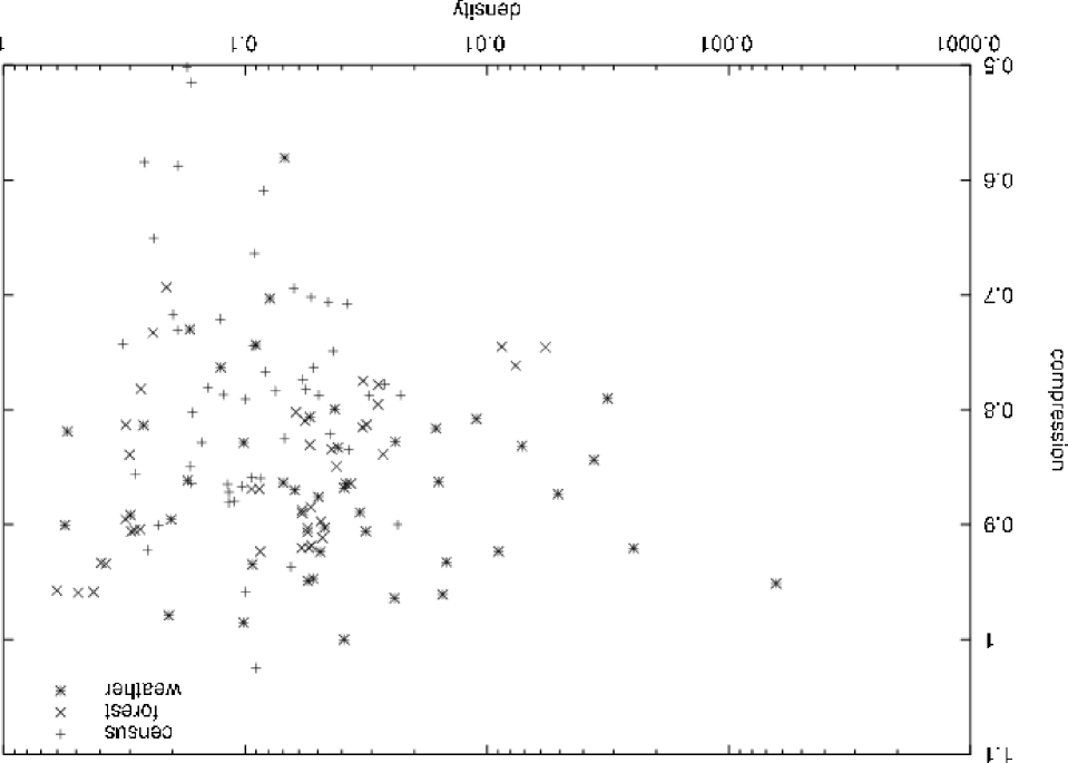
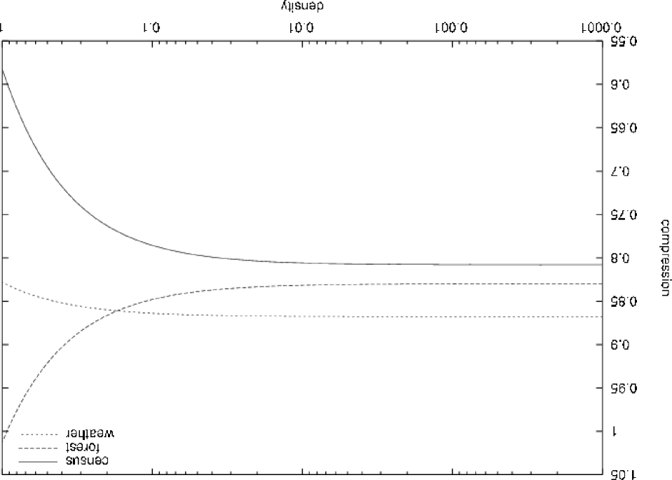
Figure 8: Compression ratios achieved with IM versus density for 50 test runs on three data sets. The bottom plot shows linear regression on a logarithmic scale: both Census and Weather showed a tendency to better compression with higher density.

7.2.3 Comparison with Pure ROLAP Coding

To place the efficiency gains from normalization into context, we calculated (for each of the 50 Census cubes) $c_{\rm default}$, the HOLAP storage cost using 2-regular blocks and the default normalization. We also calculated $c_{\rm ROLAP}$, the ROLAP cost, for each cube. The average of the 50 ratios $\frac{c_{\rm default}}{c_{\rm ROLAP}}$ was 0.69 with a standard deviation of 0.14. In other words, block-coding was 31% more efficient than ROLAP. On the other hand, we have shown that normalization brought gains of about 19% over the default normalization and the storage ratio itself was brought from 0.69 to 0.56 in going from simple block coding to block coding together with optimized normalization. Forest and Weather were similar, and their respective average ratios $\frac{c_{\rm default}}{c_{\rm ROLAP}}$ were 0.69 and 0.81. Their respective normalization gains were about 14% and 12%, resulting in overall storage ratios of about 0.60 and 0.71, respectively.

8 Conclusion

In this paper, we have given several theoretical results relating to cube normalization. Because even simple special cases of the problem are NP-hard, heuristics are needed. However, an optimal normalization can be computed when $1\times 2$ blocks are used, and this forms the basis of the IM heuristic, which seemed most efficient in experiments. Nevertheless, a Frequency Sort algorithm is much faster, and another of the paper’s theoretical conclusions was that this algorithm becomes increasingly optimal as the Independence Sum of the cube increases: if dimensions are nearly statistically independent, it is sufficient to sort the attribute values for each dimension separately. Unfortunately, our theorem did not provide a very tight bound on suboptimality. Nevertheless, we determined experimentally that an Independence Sum greater than 0.72 always meant that Frequency Sort produced good results.

As future work, we will seek tighter theoretical bounds and more effective heuristics for the cases when the Independence Sum is small. We are implementing the proposed architecture by combining an embedded relational database with a C++ layer. We will verify our claim that a more efficient normalization leads to faster queries.

References

- [1] O. Kaser, D. Lemire, Attribute-value reordering for efficient hybrid OLAP, in: DOLAP, 2003, pp. 1–8.
- [2] S. Goil, High performance on-line analytical processing and data mining on parallel computers, Ph.D. thesis, Dept. ECE, Northwestern University (1999).
- [3] F. Dehne, T. Eavis, A. Rau-Chaplin, Coarse grained parallel on-line analytical processing (OLAP) for data mining, in: ICCS, 2001, pp. 589–598.
- [4] W. Ng, C. V. Ravishankar, Block-oriented compression techniques for large statistical databases, IEEE Knowledge and Data Engineering 9 (2) (1997) 314–328.
- [5] Y. Sismanis, A. Deligiannakis, N. Roussopoulus, Y. Kotidis, Dwarf: Shrinking the petacube, in: SIGMOD, 2002, pp. 464–475.
- [6] Y. Zhao, P. M. Deshpande, J. F. Naughton, An array-based algorithm for simultaneous multidimensional aggregates, in: SIGMOD, ACM Press, 1997, pp. 159–170.
- [7] D. W.-L. Cheung, B. Zhou, B. Kao, K. Hu, S. D. Lee, DROLAP - a dense-region based approach to on-line analytical processing, in: DEXA, 1999, pp. 761–770.
- [8] D. W.-L. Cheung, B. Zhou, B. Kao, H. Kan, S. D. Lee, Towards the building of a dense-region-based OLAP system, Data and Knowledge Engineering 36 (1) (2001) 1–27.
- [9] O. Kaser, Compressing MOLAP arrays by attribute-value reordering: An experimental analysis, Tech. Rep. TR-02-001, Dept. of CS and Appl. Stats, U. of New Brunswick, Saint John, Canada (Aug. 2002).
- [10] D. Barbará, X. Wu, Using loglinear models to compress datacube, in: Web-Age Information Management, 2000, pp. 311–322.
- [11] J. S. Vitter, M. Wang, Approximate computation of multidimensional aggregates of sparse data using wavelets, in: SIGMOD, 1999, pp. 193–204.
- [12] M. Riedewald, D. Agrawal, A. El Abbadi, pCube: Update-efficient online aggregation with progressive feedback and error bounds, in: SSDBM, 2000, pp. 95–108.
- [13] S. Sarawagi, M. Stonebraker, Efficient organization of large multidimensional arrays, in: ICDE, 1994, pp. 328–336.
- [14] J. Li, J. Srivastava, Efficient aggregation algorithms for compressed data warehouses, IEEE Knowledge and Data Engineering 14 (3).
- [15] D. S. Johnson, A catalog of complexity classes, in: van Leeuwen [24], pp. 67–161.
- [16] J. van Leeuwen, Graph algorithms, in: Handbook of Theoretical Computer Science [24], pp. 525–631.
- [17] M. R. Garey, D. S. Johnson, Computers and Intractability: A Guide to the Theory of NP-Completeness, W. H. Freeman, New York, 1979.
- [18] H. B. Hunt, III, D. J. Rosenkrantz, Complexity of grammatical similarity relations: Preliminary report, in: Conference on Theoretical Computer Science, Dept. of Computer Science, U. of Waterloo, 1977, pp. 139–148, cited in Garey and Johnson.
- [19] H. Gabow, An efficient implementation of Edmond’s algorithm for maximum matching on graphs, J. ACM 23 (1976) 221–234.
- [20] R. K. Ahuja, T. L. Magnanti, J. B. Orlin, Network Flows: Theory, Algorithms, and Applications, Prentice Hall, 1993.
- [21] O. Kaser, Compressing arrays by ordering attribute values, Information Processing Letters 92 (2004) 253–256.
- [22] S. Hettich, S. D. Bay, The UCI KDD archive, http://kdd.ics.uci.edu, last checked on 26/8/2005 (2000).
- [23] C. Hahn, S. Warren, J. London, Edited synoptic cloud reports from ships and land stations over the globe (1982-1991), http://cdiac.esd.ornl.gov/epubs/ndp/ndp026b/ndp026b.htm, last checked on 26/8/2005 (2001).
- [24] J. van Leeuwen (Ed.), Handbook of Theoretical Computer Science, Vol. A, Elsevier/ MIT Press, 1990.