[cs/0702125] Bayesian Network Tomography and Inference

1 Abstract

The aim of this technical report is to give a short overview of known techniques for network tomography (introduced in the paper of Vardi (1996)), extended by a Bayesian approach originating Tebaldi and West (1998). Since the studies of A.K. Erlang (1878-1929) on telephone networks in the last millennium, lots of needs are seen in todays applications of networks and network tomography, so for instance networks are a critical component of the information structure supporting finance, commerce and even civil and national defence. An attack on a network can be performed as an intrusion in the network or as sending a lot of fault information and disturbing the network flow. Such attacks can be detected by modelling the traffic flows in a network, by counting the source destination packets and even by measuring counts over time and by drawing a comparison with this ’time series’ for instance.

2 Introduction

In order to know, find and understand the typical denial of service attack, it is necessary to understand the principle of protocols transmitted over a network. As an example we can look at the TCP protocol. The TCP-header is illustrated in figure 1.

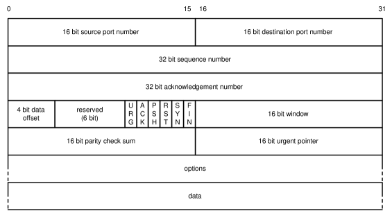
Refer to caption — Abbildung 1: The TCP segment

One of the main features of TCP is the concept of ports. Each session to or from an application is assigned a source port and a destination port. A source destination port pairing is used to disambiguate multiple ongoing sessions between machines. TCP also implements a two way connection scheme based on the usage of flags in the header. A common interaction on a network will be, that the client sends a packet with a synchronize flag set indication a communication. The destination then opens a port for the communication based on that request. The server is responding with both a synchronize and an acknowledgement flag and then finally the client responds with an acknowledgement flag. This is the three way handshake (see figure 2),

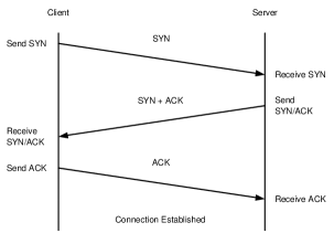
which sets up the connection and allows a two way communication (description in a very simply way). One idea of an attack is to flood a computer with bogus requests or to cause it to devote resources to the attack at the expense of the legitimate user of the system. The attacker is just sending packets that request for a communication but never completes the three way handshake. Another attack is to send packets via the network that are full of errors so that the victim computer is forced to spend time with these errors. This results in a number of reset (or other) packets with no obvious session.
We are able to compute detection probabilities in the following way (see Marchette (2005) and Moore et al. (2001)). IP addresses are unique 32-bit numeric address of every host and router on the Internet. „Spoofing“ denotes the changing of the source address to a nonexistent address. We simply collect the packets with no obvious session. Assume the spoofed IP addresses are generated randomly, uniformly and independently on all $2^{32}$ addresses. We assume that $d$ packets are sent in an attack on a victim in a network. If we monitor all packets to IP addresses, the probability of detecting an attack is given by

\displaystyle P(\textrm{'detect an attack'})=1-\left(1-\frac{w}{2^{32}}\right)^{d}

with expected number of disturbing packets is given by

\displaystyle\frac{wd}{2^{32}},

where $w$ denotes the number of monitored IP addresses. To infer how many packets were originally sent we need to estimate the severity of an attack. Under the assumption of independence probability of defining $j$ packets as attacking packets is given by

\displaystyle P(j\textrm{ 'packets'})={d\choose j}\left(\frac{w}{2^{32}}\right)^{j}\left(1-\frac{w}{2^{32}}\right)^{d-j}

and the maximum likelihood estimate for $d$ is given by

\displaystyle\hat{d}=\left\lfloor\frac{j\,2^{32}}{w}\right\rfloor.

So if we see $j$ packets, we can estimate the number of such attacks. From the literature it is known that the assumption of independence the number of attack packets between two detected packets, is given by

\displaystyle\sum_{s=1}^{w}s\left(1-\frac{w}{N}\right)^{s-1}\frac{w}{N},

where $N$ is the number of IP addresses used for randomly simulating those IP addresses that are used by an attacker, $w$ is the number of monitored IP addresses.
Another more sophisticated approach will be in monitoring and modelling the behaviour of the packets in the flow through the network. Looking at the traffic we want to estimate the network flow intensity. The aim will be to estimate the traffic intensities by two ways. First we are able to measure source destination (directed) pairs of nodes and then perform repeated measurements on the nodes to count packets (for example phone calls in routing, emails and so on) transmitted over a communication network. One main assumption in our mathematical model is, that we deal with a strongly connected network, which means, that there always exists a directed path between any two nodes.
When we study the architecture of networks, we distinguish between two main groups of networks – those that are deterministic (fixed routing) networks and those that are random (Markovian routing) networks. In the first group we deal with directed paths between the nodes, that are fixed and known for each communication. For the second group the travelling of information (sending of packets) is determined by a fixed known Markov chain. It can be easily seen that random routing is a special case of fixed routing.
A source destination pair (short SD) transports information from the source to the destination over a direct connected path in the network. We introduce $c$ as the number of SD pairs, which can be calculated from the number of nodes $n$ by

\displaystyle c=(n-1)n.

The number of transmitted information of a SD pair $j$ at measurement period $k$ is given by $X_{j}^{(k)}$ , which, like in classical teletraffic theoryïs assumed to follow a Poisson distribution with parameter $\lambda_{j}$ , i.e.

\displaystyle X_{j}^{(k)}\sim\textrm{Po}(\lambda_{j}).

We can formulate the SD transmission vector at period $k$ by $\mathbf{X}^{(k)}=(X_{1}^{(k)},...,X_{c}^{(k)})^{t}$ . For the modelling of the problem we need to introduce the $r\times c$ routing matrix $\mathbf{A}$ for a deterministic network as a $(0,1)$ -matrix given by

\displaystyle\mathbf{A}=(a_{ij}).

We get $a_{ij}=1$ if the link $i$ belongs to the directed path of the SD pair and $a_{ij}=0$ if the link $i$ does not belong to the directed path of the SD pair.

Vardi (1996) gives several example networks, for instance such network is given in figure 3.

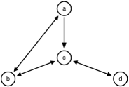
It is a four-node directed network and consists of

c=(n-1)\cdot n=3\cdot 4=12

SD pairs and seven directed links.
For better reading the routing matrix $\mathbf{A}$ is given for better reading in the table 1 with $Y_{i}$ and $X_{j}$ describing the structure displayed in table 2.

$\mathbf{A}$	$X_{1}$	$X_{2}$	$X_{3}$	$X_{4}$	$X_{5}$	$X_{6}$	$X_{7}$	$X_{8}$	$X_{9}$	$X_{10}$	$X_{11}$	$X_{12}$
$Y_{1}$	1	0	0	0	0	0	0	0	0	0	0	0
$Y_{2}$	0	1	1	0	0	1	0	0	0	0	0	0
$Y_{3}$	0	0	0	1	0	1	1	0	0	1	0	0
$Y_{4}$	0	0	0	0	1	0	0	0	0	0	0	0
$Y_{5}$	0	0	0	0	0	0	1	1	0	1	1	0
$Y_{6}$	0	0	1	0	0	1	0	0	1	0	0	0
$Y_{7}$	0	0	0	0	0	0	0	0	0	1	1	1

Tabelle 1: Routing matrix

\mathbf{A}

	$Y_{1}:\;a\rightarrow b$		$X_{1}:\;a\rightarrow b$
	$Y_{2}:\;a\rightarrow c$		$X_{2}:\;a\rightarrow c$
	$Y_{3}:\;b\rightarrow a$		$X_{3}:\;a\rightarrow c\rightarrow d$
	$Y_{4}:\;b\rightarrow c$		$X_{4}:\;b\rightarrow a$
	$Y_{5}:\;c\rightarrow b$		$X_{5}:\;b\rightarrow c$
	$Y_{6}:\;c\rightarrow d$		$X_{6}:\;b\rightarrow a\rightarrow c\rightarrow d$
	$Y_{7}:\;d\rightarrow c$		$X_{7}:\;c\rightarrow b\rightarrow a$
			$X_{8}:\;c\rightarrow b$
			$X_{9}:\;c\rightarrow d$
			$X_{10}:\;d\rightarrow c\rightarrow b\rightarrow a$
			$X_{11}:\;d\rightarrow c\rightarrow b$
			$X_{12}:\;d\rightarrow c$

Tabelle 2: Structure represented in

\mathbf{A}

The measured data on all links of the network is given by $\mathbf{Y}^{(k)}=(Y_{1}^{(k)},...,Y_{r}^{(k)})$ , where $r$ denotes all directed links in the network with the property $r=O(n)$ and $c>r$ . The formulation of the network model is given by

\mathbf{Y}=\mathbf{AX}

(1)

and if we consider measurement periods $k$ , we rewrite this as

\displaystyle\mathbf{Y}^{(k)}=\mathbf{A}\mathbf{X}^{(k)}.

The goal is to estimate $\boldsymbol{\lambda}=(\lambda_{1},...,\lambda_{c})$ from $\mathbf{Y}^{(1)},...,\mathbf{Y}^{(k)}$ . The following questions turn up:

–

Are the parameters identifiable?
–

Are the estimates consistent?

The model we deal with is a linear one, but we cannot use a linear regression nor a random effect model because we deal with a $(0,1)$ -matrix $\mathbf{A}$ , nonnegativity constraints on the parameters and the Poisson assumption for the number of transmitted messages.
The identifiability of the parameter vector $\boldsymbol{\lambda}$ can be easily verified by the following lemma (see Vardi (1996)).

Lemma If the columns of the routing matrix $\mathbf{A}$ are all distinct and each column has at least one non-zero entry $a_{ij}$ , then $\boldsymbol{\lambda}$ is identifiable.

The proof follows the principle of induction and we refer to Vardi (1996). If we find a zero column in the routing matrix $\mathbf{A}$ , we can conclude that the corresponding SD pair is not connected by a path, and if there is a zero row, then the corresponding link is not a part of the network. This observations leads us to the following assertion:

Lemma If $c>2^{r}-1,$ then some rates $\lambda_{1},...,\lambda_{c}$ cannot be estimated separately.

3 Parameter Estimation

With this model setting we can apply classical maximum likelihood estimation (MLE), also iterative expectation maximisation (EM) algorithms are also proposed in the literature. Using maximum likelihood estimation we can expect problems due to the nonlinear constraints. The structure of the log-likelihood function, which is to maximised, is hard to evaluate. The likelihood equations read

\displaystyle\frac{\partial l}{\partial\lambda_{i}}=0\textrm{ for }i=1,...,c,

where $l$ denotes the logarithm of the likelihood function $L$ . In vector notation this can be expressed as

\displaystyle\frac{1}{K}\sum_{k=1}^{K}E_{\boldsymbol{\lambda}}[\mathbf{X}^{(k)}|\mathbf{Y}^{(k)}=\mathbf{A}\mathbf{X}^{(k)}]-\boldsymbol{\lambda}=0

$\mathbf{X}^{(k)}$ are the complete (unobserved) data and $\mathbf{Y}^{(k)}$ are the incomplete (observed) data. A formulation of the EM algorithm under the assumption of independence of the $k$ components is given by

\displaystyle\boldsymbol{\lambda}^{(n+1)}=\frac{1}{K}\sum_{k=1}^{K}E[\mathbf{X}^{(k)}|\mathbf{Y}^{(k)},\boldsymbol{\lambda}^{(n)}].

A problem which we mark out here is, that the above given summands are hard to calculate, since the solutions are located in the integer range. For finding a maximum it is necessary, that the log-likelihood is concave. By evaluating the Hessian matrix $\mathbf{H}$ given by

\displaystyle\mathbf{H}=(\frac{\partial^{2}l}{\partial\lambda_{i}\partial\lambda_{j}}),

we see that this matrix is not necessarily negative semidefinite, so $l$ is not necessarily concave (see Vardi (1996)). A resolution of this problem is given by the following proposition

Proposition 1 If $\boldsymbol{\lambda}^{\ast}$ is an interior point, then for large $K$ , $l$ is concave in the neighbourhood of $\boldsymbol{\lambda}^{\ast}$ .

Other estimation methods instead of MLE are based on normal approximations. Under the assumption of normality:

\displaystyle\mathbf{X}\sim N(\boldsymbol{\lambda},\mathbf{\Lambda}),

where $\mathbf{\Lambda}=\textrm{diag}(\boldsymbol{\lambda})$ is a $c\times c$ matrix, the joint distribution of $(\mathbf{X}^{t},\mathbf{Y}^{t})^{t}$ assuming $\mathbf{Y}=\mathbf{AX}$ to hold is given by

\displaystyle\left(\begin{array}[]{c}\mathbf{X}\\ \mathbf{Y}\end{array}\right)=N_{c+r}\left(\left(\begin{array}[]{c}\boldsymbol{\lambda}\\ \mathbf{A}\boldsymbol{\lambda}\end{array}\right),\left(\begin{array}[]{cc}\boldsymbol{\lambda}&\mathbf{\Lambda}\mathbf{A}^{t}\\ \mathbf{A\Lambda}&\mathbf{A\Lambda}\mathbf{A}^{t}\end{array}\right)\right).

The conditional distribution of $\mathbf{X}$ given $\mathbf{Y}$ is given by

\displaystyle\mathbf{X}|\mathbf{Y}\sim N_{c}(\boldsymbol{\lambda}+\mathbf{\Lambda}\mathbf{A}^{t}(\mathbf{A\Lambda A})^{-1}(\mathbf{Y}-\mathbf{A}\boldsymbol{\lambda}),\mathbf{\Lambda}-\mathbf{A}^{t}(\mathbf{A\Lambda}\mathbf{A}^{t})^{-1}\mathbf{A\Lambda})

so we are able to approximate

\displaystyle E[\mathbf{X}|\mathbf{Y},\boldsymbol{\lambda}]\approx\boldsymbol{\lambda}+\mathbf{\Lambda}\mathbf{A}^{t}(\mathbf{A\Lambda A}^{t})^{-1}(\mathbf{Y}-\mathbf{A\Lambda})

and get the following iteration formulae

\displaystyle\boldsymbol{\lambda}^{(n+1)}=\frac{1}{K}\sum_{k=1}^{K}[\boldsymbol{\lambda}^{(n)}+\mathbf{\Lambda}^{(n)}\mathbf{A}^{t}(\mathbf{A\Lambda}^{(n)}\mathbf{A}^{t})^{-1}(\mathbf{Y}^{(k)}-\mathbf{A}\boldsymbol{\lambda}^{(n)})].

At this point we should mention, that a priori all $\lambda_{i}>>0$ . Here we have to expect nonnegligible approximation errors. Because of the matrix inversion some of the $\boldsymbol{\lambda}^{(i+1)}$ can be negative. Another approach that has been proposed in the literature is to assume the sum of the $\mathbf{Y}^{(k)}$ to be normally distributed,

\displaystyle\bar{\mathbf{Y}}=\frac{1}{K}\sum_{k=1}^{K}\mathbf{Y}^{(k)}\sim N_{r}(\mathbf{A}\boldsymbol{\lambda},K^{-1}\mathbf{A\Lambda A}^{t}).

The log-likelihood of $\bar{\mathbf{Y}}$ is given by

\displaystyle l(\boldsymbol{\lambda})=-\log|\mathbf{A\Lambda A}^{t}|-K(\bar{\mathbf{Y}}-\mathbf{A}\boldsymbol{\lambda})^{t}(\mathbf{A\Lambda A}^{t})^{-1}(\bar{\mathbf{Y}}-\mathbf{A}\boldsymbol{\lambda})\rightarrow\max_{\lambda_{i}\geq 0}.

Another approach to the estimation problem is based on sample moments where $\bar{\mathbf{Y}}$ is completely determined by the mean vector $\mathbf{A}\boldsymbol{\lambda}$ and the covariance matrix $\mathbf{A\Lambda A}^{t}$ of $\mathbf{Y}$ and under the usage of the first and second moment we get

•

$\widehat{E(\mathbf{Y})}=\bar{\mathbf{Y}}=\mathbf{A}\boldsymbol{\lambda}$
•

$\textrm{Cov}(Y_{i},Y_{h})=\frac{1}{K}\sum_{k}Y_{i}^{(k)}Y_{h}^{(k)}-\bar{Y_{i}}\bar{Y_{h}}=\sum_{l=1}^{c}a_{il}a_{hl}\lambda_{l}$ for $1\leq i\leq h\leq r$

where the first moment equation is independent of the Poisson assumption and the second moment equation strongly depends on the Poisson model.

4 Prior Models for Network Tomography

In this section we will investigate the problem of computing and summarizing the joint posterior distribution of $p(\mathbf{X}|\mathbf{Y})$ for all observed messages of SD pairs given the observed link counts $\mathbf{Y}$ . For the posterior distribution we need a model for the prior distribution $p(\mathbf{X})$ to be tied together with $\mathbf{Y}=\mathbf{AX}$ . Under the assumption, that the $X_{j}$ are independently Poisson distributed over the routs $j$ , the prior specification is completed by a prior of $\mathbf{\Lambda}$ . The joint distribution of the model is then given by

\displaystyle p(\mathbf{X},\mathbf{\Lambda})=p(\mathbf{\Lambda})\prod_{j=1}^{c}\lambda_{j}^{X_{j}}e^{\frac{-\lambda_{j}}{X_{j}!}}.

We are interested in estimation of $\mathbf{X}$ since we can infer $\mathbf{X}$ and $\mathbf{\Lambda}$ from the joint distribution. On a more advanced modelling standard we can also use hierarchical modeling for the parameters $\lambda_{i}$ . It is common in literature to model such hyperparameters by a normal distribution $N(\mu,\sigma)$ . Posterior computations are difficult to evaluate analytically. For example, it is unrealistic to evaluate them for large networks. For this purpose we introduce some iterative MCMC simulation algorithms. As an example consider Gibbs sampling, which iteratively resamples from the conditional posterior for elements of the $\mathbf{X}$ and $\mathbf{\Lambda}$ variables. Under the usage of

\displaystyle p(\mathbf{\Lambda}|\mathbf{X,Y})=p(\mathbf{\Lambda}|\mathbf{X})=\prod_{j=1}^{c}p(\lambda_{j}|X_{j}),

whose components have the form of the prior density $p(\lambda_{j})$ multiplied by a gamma function arising in the Poisson based likelihood function. It is possible to simulate new $\mathbf{\Lambda}$ values as a set of independent drawing from the univariate posterior density. If the prior densities are gamma densities or a mixture of gamma densities, these drawings are trivially made from the corresponding gamma or mixed gamma posterior densities. Otherwise, as proposed in literature, we have to use the rejection method or embedded Metropolis Hasting steps in the MCMC scheme in the standard Metropolis - Gibbs framework.
The theoretical structure of a general network model leads to the following theoretical result for computing samples from the conditional posteriors. Let $\mathbf{\Lambda}$ be fixed and focus on the conditional posterior $p(\mathbf{X}|\mathbf{\Lambda,Y})$ , then we can use the following theorem due to Tebaldi and West (1998).

Proposition 2 In the network model $\mathbf{Y}=\mathbf{AX}$ and under the assumption that $\mathbf{A}$ has full rank $r$ , we can reorder the columns of $\mathbf{A}$ such, that the revised routing matrix has the form

\displaystyle\mathbf{A}=[\mathbf{A}_{1},\mathbf{A}_{2}]

where $\mathbf{A}_{1}$ is a nonsingular $r\times r$ matrix. By similar reordering the elements of the vector $\mathbf{X}$ and partitioning as $\mathbf{X}^{t}=(\mathbf{X}_{1}^{t},\mathbf{X}_{2}^{t})$ , it follows that

\displaystyle\mathbf{X}_{1}=\mathbf{A}_{1}^{-1}(\mathbf{Y}-\mathbf{A}_{2}\mathbf{X}_{2}).

This result easily follows from the fact that $\mathbf{Y}=\mathbf{AX}=\mathbf{A}_{1}\mathbf{X}_{1}+\mathbf{A}_{2}\mathbf{X}_{2}$ .

The full rank assumption is satisfied by all networks in real world. Otherwise there is a redundancy in specification, and one or more rows of $\mathbf{A}$ can be deleted to get linear independent rows. The result in the last proposition implies that, given $\mathbf{Y}$ and the assumed values of the $(c-r)$ route counts in $\mathbf{X}_{2}$ , we are able to compute directly the remaining $r$ route flows simply based on the algebraic structure of the routing matrix. For the reordering of the matrix $\mathbf{A}$ we can use the QR decomposition of arbitrary full rank matrices. After the QR decomposition we get an $r\times r$ orthogonal matrix $\mathbf{Q}$ and an $r\times c$ upper triangular matrix $\mathbf{R}$ , the first $r$ columns of which correspond to $r$ linear independent columns of $\mathbf{A}$ . These are identified by a permutation of column indices.
With this knowledge we can deduce, that the conditional distribution $p(\mathbf{X}|\mathbf{\Lambda,Y})$ lies in the $c-r$ dimensional subspace defined by the partition $\mathbf{A}=[\mathbf{A}_{1},\mathbf{A}_{2}]$ . After the partitioning of the routing matrix $\mathbf{A}$ the posterior has the form

\displaystyle p(\mathbf{X_{1}|X_{2},\Lambda,Y})p(\mathbf{X_{2}|\Lambda,Y}),

where $p(\mathbf{X_{1}|X_{2},\Lambda,Y})$ is degenerated at $\mathbf{X_{1}=A_{1}^{-1}(Y-A_{2}X_{2})}$ with $\mathbf{X}_{2}=(X_{r+1},..,X_{c})^{t}$ and $\mathbf{X}_{1}=(X_{1},...,X_{r})^{t}$ defined as above. The conditional is given by

p(\mathbf{X_{2}|\Lambda,Y})\propto\prod_{a=1}^{c}\frac{\lambda_{a}^{X_{a}}}{X_{a}!}

with the support defined by $X_{a}\geq 0$ for all $a=1,\ldots,c$ . It is the product of independent Poisson priors for the $X_{i}$ constrained by the model and the reordering. The utility of this expression is in delivering the set of complete conditional posteriors for elements of the $\mathbf{X_{2}}$ vector to form a part of the iterative simulation approach to posterior analysis. Let´s now consider each element $X_{i}$ of $\mathbf{X_{2}},(i=r+1,\ldots,c)$ , and write $\mathbf{X_{2,-i}}$ for the remaining elements. The conditional distribution $p(X_{i}|\mathbf{X_{2,-i},\Lambda,Y})$ is given by

p(X_{i}|\mathbf{X_{2,-i},\Lambda,Y})\propto\frac{\lambda_{i}^{X_{i}}}{X_{i}!}\prod_{a=1}^{r}\frac{\lambda_{a}^{X_{a}}}{X_{a}!},

over the support of the expression above. The linear constraints on $X_{i},i\in\{r+1,\ldots,c\}$ , are of the form $X_{i}\geq d_{i}$ and $X_{i}\leq e_{i},$ where the values $d_{i}$ and $e_{i}$ are functions of the conditioning values of $\mathbf{X_{2,-i}}$ and $\mathbf{Y}$ . Together with $X_{i}\geq 0$ we obtain at most a set of $r+1$ constraints on $X_{i}$ . It is computationally very burdensome to evaluate directly these constraints and identify their intersection. So we can make direct simulations.
For the simulation of the full posterior $p(\mathbf{X,\Lambda|Y})$ we need now fixed starting values of the route counts $\mathbf{X}$ . We can apply the following algorithm according to Tebaldi and West (1998):

Algorithm

1.

Draw sampled values of the rates $\mathbf{\Lambda}$ from $c$ conditionally independent posteriors $p(\lambda_{a}|X_{a}),$
2.

conditioning on these values of $\mathbf{\Lambda}$ simulate a new $\mathbf{X}$ vector by sequencing through $i=r+1,\ldots,c$ , and at each step sample a new $X_{i}$ with the conditioning elements from the $\mathbf{X_{2,-i}}$ set at their most recent sampled values,
3.

iterate.

This is a known standard Gibbs sampling setup. Scalar elements of both $\mathbf{\Lambda}$ and $\mathbf{X}$ are resampled from the relevant distribution conditional on most recently simulated values of all other uncertain quantities. In step 2 we require evaluation of the support which is best done by a simulation method such as embedded Metropolis-Hastings steps. We note that from $\mathbf{Y=AX}$ it is possible to identify bounds on each $X_{i}$ . A suitable range for the proposal distribution can be computed from that.

5 Usage of Bayes Factors for Modelling of Network Traffic

If there is a sequence of packets transmitted over a network, we can evaluate a statistical profile of that sequence based on the information of the header and compare this to similar sequences in the past. This historical behaviour can be saved in a stochastic matrix where each element of the matrix is given by

\displaystyle p_{jku}=P(\textrm{'SD'}=k|\textrm{'SD before'}=j,\textrm{'IP of sender'}=u)

Since we know the header in the packet, we are able to model the behaviour of the sender over time. We can base an analysis on these matrices. DuMouchel (1999) has made a similar approach for modelling of the behaviour of commands in a shell. Since we use some kind of categorical data, we are able to use the multinomial distribution as proposed in the literature. For Bayesian inference we can use the Dirichlet (prior) distribution, which is the natural conjugate distribution to the multinomial distribution.
Let $\mathbf{p}=(p_{1},...,p_{K})$ be a random vector which is Dirichlet distributed with the density

\displaystyle f(\mathbf{p})=\frac{\Gamma(\sum_{k}\alpha_{k})\prod_{k}(p_{k}^{\alpha_{k-1}})}{\Gamma(\alpha_{k})}

with $\alpha_{i}>0$ for all $i$ . The multinomial probability for a count data vector $\mathbf{n}=(n_{1},...,n_{K})$ with $\tilde{n}=\sum_{k}n_{k}$ is given by

\displaystyle P(n|p)=\tilde{n}!\prod_{k}\frac{p_{k}^{n_{k}}}{n_{k}!}

From above formulas we get the marginal distribution

\displaystyle P(n)=\frac{\tilde{n}!}{\tilde{\alpha}(\tilde{\alpha}+1)\cdot\ldots\cdot(\tilde{\alpha}+\tilde{n}-1)}\prod_{k}\frac{\alpha_{k}(\alpha_{k}+1)\cdot\ldots\cdot(\alpha_{k}+n_{k}-1)}{n_{k}!}

with $\tilde{\alpha}=\sum_{k}\alpha_{k}$ . The posterior distribution is given by the following Dirichlet distribution

\displaystyle P(p|n)=(\tilde{\alpha}+\tilde{n}-1)!\prod_{k}\frac{p_{k}^{n_{k}+\alpha_{k}-1}}{(\alpha_{k}+n_{k}-1)!}

On the idea that one user $u$ in the network generates a sequence of $T+1$ packets $C_{0},C_{1},...,C_{T}$ we can build the following hypotheses for a test of sending packets that disturb the network

	$\displaystyle H_{0}:P(C_{t}=k\|C_{t-1}=j)=p_{jku}$
	$\displaystyle H_{1}:P(C_{t}=k\|C_{t-1}=j)=Q_{k}$

where

\displaystyle(Q_{1},...,Q_{k})\sim\textrm{Dirichlet}(\alpha_{01},...,\alpha_{0k}).

We make the assumption that the null hypothesis $H_{0}$ says that a legitimate user is generating packets out of the profiles of the transition probabilities. The alternative hypothesis $H_{1}$ says, that $T$ packets are sent through the network, are drawn randomly and independently from a probability vector following a Dirichlet distribution with given hyperparameters. These hyperparameters have to be estimated. $H_{1}$ is more general than $H_{0}$ since we do not know $Q$ in comparison with the fully specified $\mathbf{P}_{u}=(p_{jku})$ . $H_{0}$ is not nested in $H_{1}$ . For checking the practicability we suggest the usage of Bayes factors $BF$ given by

\displaystyle BF=\frac{P(C_{0},...,C_{T}|H_{1})}{P(C_{0},...,C_{T}|H_{0})}

for inference. For large $BF$ we will prefer the alternative hypotheses. Instead of BF often

\displaystyle x=\log(BF)

is used, which is called the ”weight of evidence”. We can see that modelling the behaviour using the network with the network tomography and combining it with the concepts of Bayes factors we are able to implement a large apparatus for monitoring networks and to draw a conclusion whether there is an attack on our monitored network.

6 Conclusions

In this paper we gave an overview of the current literature in network modelling and network tomography. We extended that field by developing a method for monitoring networks with Bayes factors for testing hypothesis testing whether there is an intruder in the network, who performs several forms of attacks. This method can be implemented with the usage of control charts which are common in quality control for monitoring networks. Further work will be in random routing networks – for an overview of current applications we refer to Vardi (1996). The methodologies developed here should be also applicable for these kinds of networks. Results and implementation will be given in further technical reports.

7 References

Castro, R., Coates, M., Liang, G., Nowak, R., Yu,B.: (2004) Network Tomography: Recent Developments. Statistical Science 19 (3): 499–517
DuMouchel, W.: (1999) Computer Intrusion Detection Based on Bayes Factors for Comparing Command Transition Probabilities. National Institute of Statistical Sciences (NISS), Technical Report Number 91
Marchette, D. J.: (2001) Computer Intrusion Detection and Network Monitoring: A Statistical Viewpoint. New York: Springer
Marchette, D. J.: (2005) Passive Detection of Denial of Service Attacks on the Internet. In: Statistical Methods in Computer Security. Dekker: New York
McCulloch, R.: (1998) Bayesian Inference on Network Traffic Using Link Count Data: Comment. Journal of the American Statistical Association 93 (442): 575
Moore, D., Voelker, G.M., Savage, S.: (2001) Inferring Internet Denial-of-Service Activity. USENIX Security Symposium’01. www.usenix.org/publications
/library/proceedings/sec01/moore.html
Tanenbaum, A. S.: (1996) Computer Networks. Upper Saddle River: Prentice Hall
Tebaldi, C., West, M.: (1998) Bayesian Inference on Network Traffic Using Link Count Data. Journal of the American Statistical Association 93 (442): 557–573
Vardi, Y.: (1998) Bayesian Inference on Network Traffic Using Link Count Data: Comment. Journal of the American Statistical Association 93 (442): 573–574
Vardi, Y.: (1996) Network tomography: Estimating source-destination traffic intensities from link data. Journal of the American Statistical Association 91 (433): 365–377
Willinger, W., Paxson, V.: (1998) Where mathematics meets the internet. Notices of the American Mathematical Society 45 (8): 961–970
Wakounig, S.: (2005) Einfache statistische Ansätze für Intrusion Detection Systeme. MSc Thesis. University of Klagenfurt. Department of Applied Statistics.