Observable graphs

Abstract. An edge-colored directed graph is observable if an agent that moves along its edges is able to determine his position in the graph after a sufficiently long observation of the edge colors. When the agent is able to determine his position only from time to time, the graph is said to be partly observable. Observability in graphs is desirable in situations where autonomous agents are moving on a network and one wants to localize them (or the agent wants to localize himself) with limited information. In this paper, we completely characterize observable and partly observable graphs and show how these concepts relate to observable discrete event systems and to local automata. Based on these characterizations, we provide polynomial time algorithms to decide observability, to decide partial observability, and to compute the minimal number of observations necessary for finding the position of an agent. In particular we prove that in the worst case this minimal number of observations increases quadratically with the number of nodes in the graph. From this it follows that it may be necessary for an agent to pass through the same node several times before he is finally able to determine his position in the graph. We then consider the more difficult question of assigning colors to a graph so as to make it observable and we prove that two different versions of this problem are NP-complete.

1. Introduction

Consider an agent moving from node to node in a directed graph whose edges are colored. The agent knows the colored graph but does not know his position in the graph. From the sequence of colors he observes he wants to deduce his position. We say that an edge-colored directed graph is observable if there is some observation time length after which, whatever the color sequence he observes, the agent is able to determine his position. Of course, if all edges are of different colors, or if edges with different end-nodes are of different colors, then the agent is able to determine his position after just one observation. So the interesting situation is when there are fewer colors than there are nodes.

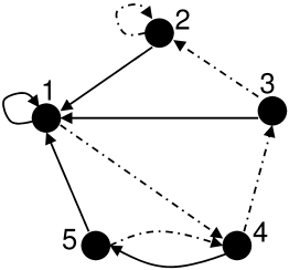
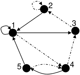
(a)	(b)

Figure 1. An agent is moving along directed edges. Edges are “colored” solid (S) or dashed (D). The graph (a) is observable because the observation of the last three colors suffices to determine the position of the agent in the graph. The graph (b) is not observable; the sequence SSDSSD$\ldots$SSD can be obtained from a path ending at node 2 or at node 4.

Consider for instance the two graphs on Figure 1. The graphs differ only by the edge between the nodes 1 and 3. The edges are colored with two “colors”: solid (S) and dashed (D). We claim that the graph (a) is observable but that (b) is not. In graph (a), if the observed color sequence is DDS then the agent is at node 1, while if the sequence is SDD he is at node 3. Actually, it follows from the results presented in this paper that the observation of color sequences of length three always suffices to determine the exact position of the agent in this graph. Consider now the graph (b) and assume that the observed sequence is SSDSS; after these observations are made, the agent may either be at node 1, or at node 3. There are two paths that produce the color sequence SSDSS and these paths have different end-nodes. Sequences of arbitrary large length and with the same property can be constructed and so graph (b) is not observable.

There are of course very natural conditions for a graph to be observable. A first condition is that no two edges of identical colors may leave the same node. Indeed, if a node has two outgoing edges with identical colors then an agent leaving that node and observing that color will not be able to determine his next position in the graph. So this is clearly a necessary condition. Another condition is that the graph may not have two cycles with identical color sequences, as for example the cycles $2-1-3-2$ and $4-5-1-4$ in graph (b) of Figure 1. If such cycles are present in the graph, then an agent observing that repeated particular color sequence is not able to determine if he is moving on one or the other cycle. So, these two conditions are clearly necessary conditions for a graph to be observable. In our first theorem we prove that these two conditions together are also sufficient.

In an observable graph there is some $T\geq 1$ for which an agent is able to determine his position in the graph for all observations of length $T$, and so he is also able to do so for all subsequent times. Some graphs are not observable in this way but in a weaker sense. Consider for example the graph (a) of Figure 2. This graph is not observable because there are two dashed edges that leave the top node and so, whenever the agent passes through that node the next observed color is D and the position of the agent is then uncertain. This graph is nevertheless partly observable because, even though the agent is not able to determine his position at all time, there is a finite window length $T$ such that the agent is able to determine his position at least once every $T$ observations. Indeed, after observing the sequence SD in this graph (and this sequence occurs in every observation sequence of length 4), the next observation is either S or D. If it is S, the agent is at the bottom right node; if it is D, he is at the bottom left node. In both cases the next observed color is S and the agent is then at the top node. So the agent is able to determine his position at least once every five observations. In an observable graph, an agent is able to determine his position at all times beyond a certain limit; in a partly observable graph the agent is able to determine his position infinitely often (for formal definitions, see below).

Notice that in the graph (a) of Figure 2, the agent is able to reconstruct its entire trajectory a posteriori, except maybe for its last position. This is however not the case for all partly observable graphs. Consider for example the star graph (b) of Figure 2. The color sequences observed in this graph are SDSDS$\ldots$ or DSDSDS$\dots$. When the last observed color is D, the agent is at the central node. When the last observed color is S, the agent only knows that he is at one of the extreme nodes. Hence this graph is partly observable but in this case, contrary to what we have with graph (a), the entire trajectory cannot be reconstructed a posteriori.

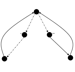
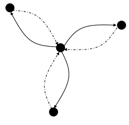
(a)	(b)

Figure 2. Both graphs are partly observable but none of them is observable. In graph (a), complete trajectories can always be reconstructed a posteriori; which is not possible in graph (b).

In this paper, we prove a number of results related to observable and partly observable graphs. We first prove that the conditions described above for observability are indeed sufficient. From the proof of this result it follows that in an observable graph an agent can determine his position in the graph after an observation of length at most $n^{2}$, where $n$ is the number of nodes. This quadratic increase of the observation length cannot be avoided: we provide a family of graphs for which $\Theta(n^{2})$ observations are necessary. Based on some of these properties we also provide polynomial-time algorithms for checking if a graph is observable or partly observable. We then consider the question of assigning colors to the edges or nodes of a directed graph so as to make it observable and we prove that the problem of finding the minimal number of colors is NP-complete.

The concept of observable graphs is related to a number of concepts in graph and automata theory, control theory and Markov models which we now describe.

Observable graphs as defined here are actually a particular case of local automata. A finite state automaton is said to be $(d,k)$-local (with $d\leq k$) if any two paths of length $k$ and identical color sequences pass through the same state at step $d$. Hence an observable graph is a $(k,k)$-local automaton. It is shown in [1] how to recognize local automata in polynomial time but the motivation in that context is very different from ours and little attention is given there at the particular values of the integer $d$ and $k$. In particular, the algorithm provided in [1] does not allow to recognize $(k,k)$-local automata.

Related to the notion of observable graphs, Crespi et al. [2] have recently introduced the concept of trackable graph. An edge-colored directed graph is said to be trackable if the maximum number of trajectories compatible with a color sequence of length $k$ grows subexponentially with $k$. So, in the context of trackability, one cares about the total number of compatible trajectories, but not about the position of the agent in the graph. It has recently been proved that the problem of determining if a graph is trackable can be solved in polynomial time [5]; see also [2]. It is clear that an observable network is trackable, but the converse is not true in general. For example the graph on Figure 2 (a) is trackable but not observable. Notice also that, as shown with the graph on Figure 2 (b), partly observable graphs do not need to be trackable.

Observable graphs are also related to Discrete Event Systems (DES). More precisely, our notion of partly observable graph is similar to what Öszveren and Willsky call observable DES [6]. These authors define DES as colored graphs, except for the fact that they allow transitions to be unobservable: some edges have no colors. From a colored graph with unobservable transitions we can easily construct an equivalent fully colored graph by removing all unobservable transitions and adding an edge $(h,j)$ of color $c$ whenever there is an edge $(h,i)$ of color $c$ and an unobservable transition (or a sequence of unobservable transitions) between $i$ and $j$. Our results are therefore applicable to observable DES as defined in [6].

Finally, the results presented in this paper can also be interpreted in the context of Hidden Markov Processes (HMP) [7, 3]. More precisely, the graphs we consider can be seen as finite alphabet HMPs (also called aggregated Markov processes), except that no values different from 0 and $1$ are given for the transition probabilities. In our context, a transition is either allowed or it is not; we do not associate transition probabilities. Also, we can assign to a given transition several possible colors, but again, without considering their respective probabilities.

The remainder of this paper is organized as follows: in Section 2 we formalize the notions presented above and give necessary and sufficient conditions for observability. Section 3 deals with algorithmic aspects: we show there how to check the conditions derived in Section 2 in polynomial time. In Section 4 we prove NP-completeness results for the design of observable and partly observable graphs. Finally, in Section 5 we conclude and describe some open questions.

2. Characterizing observability

Let $G=(V,E)$ be a graph and $C$ a set of colors. To every edge $e\in E$ we associate one (or more) color from $C$. A word $w$ on $C$ is the concatenation $w_{1}\dots w_{T}$ of symbols taken from $C$; the length $|w|$ of $w$ is the number of its symbols. A subword $w_{[i,j]}:1\leq i\leq j\leq|w|$ of $w=w_{1}\dots w_{T}$ is the concatenation of the symbols $w_{i}\dots w_{j}$. We say that a path is allowed by a word $w$ if for all $i$ the $i$th edge of the path has color $w_{i}$. Finally, for a word $w$ and a set $S\subset V$, we denote by $\delta_{w}(S)$ the set of nodes $q$ for which there exists a path allowed by $w$ beginning in a state in $S$ and ending in $q$; $\delta_{w}(V)$ is the set of nodes that can be reached from a node in $V$ with the color sequence $w$.

A graph is observable if there exists an integer $T$ such that for all words $w$ of length $|w|\geq T$, $|\delta_{w}(V)|\leq 1$. In other words there is at most one possible end-node after a path of length $T$ or more. We shall also say that a graph is partly observable if there exists an integer $T$ such that for all word $w$ with $|w|\geq T$, there exists a $1\leq t\leq T$ such that $|\delta_{w_{[1,t]}}(V)|\leq 1$.
The theorem below characterizes observable graphs. For a graph to be observable no color sequence $w$ can allow two separated cycles, that is, two cycles $\pi,\pi^{\prime}:[0,|w|]\rightarrow V$ such that $\pi(i)\neq\pi^{\prime}(i),\forall i$ and the edges $(\pi(i),\pi(i+1))$ and $(\pi^{\prime}(i),\pi^{\prime}(i+1)$ have identical colors for every $i$. For instance, the graph in Figure 1 (b) is not observable because the color sequence “solid-dashed-solid” allows both the cycle $1-3-2-1$ and the cycle $5-1-4-5$. Another condition for a graph to be observable is that no node may have two outgoing edges of the same color. This last condition only applies to the nodes of the graph that are asymptotically reachable, i.e., that can be reached by paths of arbitrary long lengths. In a strongly connected graph, all nodes are asymptotically reachable. For graphs that are not strongly connected, asymptotically reachable nodes are easy to identify in the decomposition of the graph in strongly connected components. We now prove that these two conditions together are not only necessary but also sufficient:

Theorem 1.

An edge-colored graph is observable if and only if no color sequence allows two separated cycles, and no asymptotically reachable node of the graph has two outgoing edges that have identical colors.

Proof.

$\Rightarrow:$ We prove this part by contraposition. Suppose that the first condition is violated: if we have a word $w$ allowing two separated cycles, then $ww\cdots w$ is an arbitrarily long word that allows two separated paths. Suppose now that the second condition is violated and let $v$ be an asymptotically reachable node. For any $T$, we can find a path of length $T-1$ ending in $v$ and $v$ has two outgoing edges of the same color. Let $w$ be a color sequence allowing this path, and $c$ the color of the two edges. We have then an arbitrarily long word $wc$ such that $|\delta_{wc}(V)|\geq 2$.

$\Leftarrow:$ Let us define $T_{1}$ such that every path of length larger than $T_{1}$ has its last node asymptotically reachable. We consider two arbitrary compatible paths, that is, two paths allowed by the same color sequence. We will show that they intersect between $t=T_{1}$ and $t=T_{1}+n^{\prime 2}$, with $n^{\prime}$ the number of asymptotically reachable nodes. This will establish observability of the graph, since two paths cannot split once they intersect (recall that no node has two outgoing edges of the same color), and so actually all compatible paths pass through the same node after $t=T_{1}+n^{\prime 2}$ steps. Suppose by contradiction that the two paths $\pi,\pi^{\prime}$ allowed by the same color sequence do not intersect during the last $n^{\prime 2}$ steps, when they only visit asymptotically reachable nodes. Then by the pigeonhole principle there are two instants $t_{1},t_{2}$ such that $(\pi(t_{1}),\pi^{\prime}(t_{1}))=(\pi(t_{2}),\pi^{\prime}(t_{2}))$, and the first condition is violated: $w_{[t_{1},t_{2}]}$ is a sequence that allows two separated cycles. ∎

One could think that the first condition in Theorem 1 suffices for the graph to be partly observable, but this is not the case. Consider indeed the graph in Figure 3. For notational simplicity we have put colors on the nodes rather than on the edges: one can interpret these node colors as being given to the edges incoming in the corresponding node. This graph satisfies the first condition but it is not partly observable. Indeed, the observed sequence $RGGRGG\dots$ has no subsequence allowing only one ending node.

Actually, the first condition implies a weaker notion of observability: A graph is partly a-posteriori observable if for any sufficiently long observation, it is possible a posteriori (that is, knowing the whole observation) to determine the state of the agent at at least one previous instant. We do not develop this concept any further in this paper but it should be clear that all the proofs that we provide in this and in the next section can easily be extended to cover that case as well.

The graph (a) of Figure 1 is observable and the agent can be localized after an observation of length at most 3. The above proof provides an upper bound on the observation length that is needed to localize an agent in an observable graph.

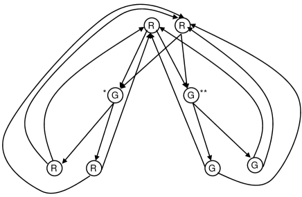
Figure 3. A graph that is not partly observable, even though no color sequence allows two separated cycles. The colors on nodes can be understood as assigned to the edges incoming in the corresponding nodes.

Corollary 1.

In an observable graph, $n^{2}-n$ observations suffice to localize an agent ($n$ is the number of nodes in the graph).

Proof.

Let us suppose by contradiction that there exists a color sequence of length $T>n^{2}-n$ that allows two paths ending in different nodes. There are $n^{2}-n$ different couples of nodes $(v_{1},v_{2}):v_{1}\neq v_{2}$ and one can follow a similar reasoning as in the previous proof to show that the graph is actually not observable. ∎

One could have expected the maximal value of $T$ to be $n$, and one may wonder whether the bound $n^{2}-n$ in the theorem is tight. We give in Section 3 a family of graphs for which the value of $T$ is $n(n-1)/2-1$; the quadratic increase can therefore not be avoided.

3. Verifying observability

In this section, we consider two algorithmic problems. The first problem is that of reconstructing the possible positions of an agent in a graph for a given sequence of color observations. That problem is easy; we describe a simple solution to it and give an example that illustrates that the bound in Corollary 1 is tight. The second problem is that of deciding observability.

Let us consider the first problem: we are given a color sequence and we would like to identify the nodes that are compatible with the observed sequence of colors. A simple algebraic solution is as follows. To every color $c$, there is an associated graph $G_{c}$ for which we can construct the corresponding adjacency matrix $A_{c}$. To a color sequence $w=w_{1},\ldots,w_{|w|}$ we then associate $A_{w}$, the corresponding product of matrices $A_{w}=A_{w_{1}}\dots A_{w_{|w|}}$. It is easy to verify that the $(i,j)$th entry of $A_{w}$ is equal to the number of paths from $i$ to $j$ allowed by $w$. The set $\delta_{w}(S)$ is therefore obtained by restricting the matrix $A_{w}$ to the lines corresponding to elements in $S$, and by taking the indices of the nonzero columns. This simple algorithm is actually nothing else than the well-known Viterbi algorithm for Hidden Markov Processes [8, 7], except that in our context the probabilities are all equal to zero or one.

As an application, let us show that the quadratic dependance for the bound in Corollary 1 cannot be improved. We describe a family of colored graphs with $n$ nodes by giving the adjacency matrices corresponding to the different colors. Our set contains $2(n-2)$ matrices. For every $1\leq i\leq n-2$ we construct two matrices: the first one, $A_{i}$, has $n-i$ entries equal to one, which are the entries $(i+1,i+2),\dots,(n-1,n),$ and $(i,i)$; the second matrix, $B_{i}$, has two entries equal to one: the entries $(i,i+1)$ and $(n,i+2)$. A colored graph defined by this set of matrices is observable (the reader can verify this by using the algorithm given below); but on the other hand the color sequence $A_{1}^{n-2}B_{1}A_{2}^{n-3}B_{2}\dots A_{n-2}B_{n-2}$, of length $n(n-1)/2-1$, allows paths that have different end nodes. This is straightforward to check by computing the corresponding product of matrices and check that it has two columns with nonzero elements.

We now turn to the main question of this section: how can one determine efficiently if a graph is observable? We have the following result.

Theorem 2.

The problems of determining whether a colored graph is observable, or partly observable, are solvable in $O(n^{4}m)$, where $n$ is the number of nodes, and $m$ is the number of colors.

Proof.

The algorithm we propose uses the conditions given in Theorem 1. We first check the condition that no color sequence allows two separated cycles. In order to do that, we construct an auxiliary directed graph that we will denote $G^{2}$ and whose nodes are couples of distinct nodes in $G$: $\{(v_{1},v_{2})\in V^{2}:v_{1}\neq v_{2}\}$. In $G^{2}$ there is an edge from $(v_{1},v_{2})$ to $(v_{1}^{\prime},v_{2}^{\prime})$ if there is a color that allows both edges $(v_{1},v_{1}^{\prime})$ and $(v_{2},v_{2}^{\prime})$. This graph can be constructed in $O(n^{4}m)$ operations, since there are less than $n^{4}$ edges in $G^{2}$ and for each of these edges we have to check $m$ colors. It is possible to design two separated cycles in $G$ allowed by the same color sequence if and only if there is one cycle in $G^{2}$. This we can test by a simple breadth first search. Now, we can check easily if an asymptotically reachable node has two outgoing edges of the same color, and determine whether the network is observable.

We now would like to test whether the graph is partly observable; in order to do that, we construct a new auxiliary directed graph $\tilde{G}^{2}$, and once again we check the existence of cycles in this graph. An easy way to obtain this new graph is to take $G^{2}$, and to add some edges: for every couple of nodes $((v_{1},v_{2}),(v_{1}^{\prime},v_{2}^{\prime}))$, we allow an edge if there is a color that allows one edge from $v_{1}$ or $v_{2}$ to $v_{1}^{\prime}$ and one edge from $v_{1}$ or $v_{2}$ to $v_{2}^{\prime}$. The graph $\tilde{G}^{2}$ can also be constructed in $O(n^{4}m)$ operations. We claim that the graph is partly observable if and only if this auxiliary graph is acyclic. Indeed, any path in the auxiliary graph ending in node, say, $(v_{1},v_{2})$ corresponds to a color sequence that allows paths ending in each of the nodes $v_{1}$ and $v_{2}$. If the auxiliary graph contains a cycle, consider the path travelling along the cycle during $T$ steps; it corresponds to a word of length $T$ such that for any $t\leq T$, the subword obtained by cutting the word at the $t$th character allows two paths ending in different nodes, and the definition of partial observability is violated. On the other hand, if the graph is not partly observable, there exist arbitrarily long sequences such that all beginning subsequence allows at least two paths ending in different nodes. This implies that $\tilde{G}^{2}$ has a cycle. Indeed, let us consider such a color sequence $\omega$ of length $T\geq n^{2}$. There are two paths $\pi,\pi_{1}:[0,T]\rightarrow V$ allowed by $\omega$ and ending in two different nodes: $\pi(T)\neq\pi_{1}(T)$. If $\pi(T-1)\neq\pi_{1}(T-1),$ then there is an edge in $\tilde{G}^{2}$ from $(\pi(T-1),\pi_{1}(T-1))$ to $(\pi(T),\pi_{1}(T))$. If $\pi(T-1)=\pi_{1}(T-1),$ then by construction of $\omega$ there exists a path $\pi_{2}$ allowed by $\omega_{[1\dots T-1]}$ that ends in a node $v_{T-1}\neq\pi(T-1).$ Thus we can iteratively define nodes $v_{i}:i\in[1,T]$ of decreasing indices $i$ such that there is a path in $\tilde{G}^{2}$ from $(v_{i-1},\pi(i-1))$ to $(v_{i},\pi(i)).$ Finally this path is of length $T$ which is more than the number of nodes in $\tilde{G}^{2},$ so this graph is cyclic. Since $\tilde{G}^{2}$ can be constructed in $O(n^{4}m)$, the proof is complete. ∎

This algorithm also allows us to compute the time necessary before localization of the agent:

Theorem 3.

In an observable graph, it is possible to compute in polynomial time the minimal $T$ such that any observation of length $T$ allows to localize the agent. The same is true for partial observability.

Proof.

Let us consider the graphs $G^{2}$ and $\tilde{G}^{2}$ in the above proof. The existence of an observation of length $T$ allowing two different last nodes (respectively, two paths with at least two different allowed nodes at every time) is equivalent to the existence of a path of length $T$ in $G^{2}$ (respectively, $\tilde{G}^{2}$). Since the auxiliary graphs are directed and acyclic, it is possible to find a longest path in polynomial time. ∎

4. Design of observable graphs is NP-complete

In this section, we prove NP-completeness results for the problem of designing observable graphs. The problem is this: we are given an (uncolored) graph and would like to color it with as few colors as possible so as to make it observable. Unless the graph is trivial, one color never suffices. On the other hand, if we have as many colors as there are nodes the problem becomes trivial. A simple question is thus: “What is the minimal number of colors that are needed to make the graph observable”? We show that this problem is NP-complete in two different situations: If we color the nodes and want to make the graph observable, or if we color the edges and want to obtain a partly observable graph. We haven’t been able to derive similar results for the other two combinations of node/edges coloring and observability/partial observability. In particular, we leave open the natural question of finding the minimal number of edge colors to make a graph observable. Even though the statements of our two results are similar, the proofs are different. In particular, we use reductions from two different NP-complete problems (3-COLORABILITY and MONOCHROMATIC-TRIANGLE).

Theorem 4.

The problem of determining, for a given graph $G$ and integer $k$, if $G$ can be made observable by coloring its nodes with $k$ colors is NP-complete.

Proof.

We have already shown how to check in polynomial time if a colored graph is observable. So the problem is in NP. In the rest of the proof we provide a polynomial-time reduction from 3-COLORABILITY to the problem of determining if a graph can be made observable by coloring its nodes with 3 colors. This will then establish the proof since 3-COLORABILITY is known to be NP-complete [4].

In 3-COLORABILITY we are given an undirected graph $G$ and the problem is to color the nodes with at most three different colors so that no two adjacent nodes have the same color. For the reduction, consider an undirected graph $G=(V,E)$. From $G$ we construct a directed graph $G^{\prime}=(V^{\prime},E^{\prime})$ such that $G^{\prime}$ can be made observable by node coloring with 3 colors if and only if $G$ is 3-colorable. Figure 4 illustrates our construction. On the left hand side we have a $3$-colorable undirected graph. The corresponding directed graph $G^{\prime}$ is represented on the right hand side. The graph $G^{\prime}$ can be made observable with three colors.

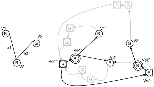
Figure 4. Construction of the graph $G^{\prime}$ and its coloration

Here is how we construct $G^{\prime}$ from $G$: For every node $v$ in $V$, we define a corresponding node $v^{\prime}$ in $V^{\prime}$ and call these nodes “real nodes”. For every edge $e=(v_{1},v_{2})$ in $E$, we define a node $v^{\prime}_{e}$ in $V^{\prime}$ and two outgoing edges $(v^{\prime}_{e},v_{1}^{\prime})$ and $(v^{\prime}_{e},v^{\prime}_{2})$. The nodes $v^{\prime}_{e}$ appear with double circles on Figure 4. The main idea of the reduction is as follows: If $G^{\prime}$ is observable by node coloring, then $v_{1}^{\prime}$ and $v_{2}^{\prime}$ cannot possibly have the same color since there are edges pointing from $v^{\prime}_{e}$ to both $v_{1}^{\prime}$ and $v_{2}^{\prime}$, and so the corresponding nodes in $G$ do indeed have different colors.

The graph $G^{\prime}$ we have constructed so far is rather simple and does not contain any cycle; in the remainder of our construction we add nodes and edges to $G^{\prime}$ so as to make it strongly connected but in such a way that the graph $G^{\prime}$ remains observable. For every node $v_{e}^{\prime}$, we add a new node $v_{e}^{\prime\prime}$ and an edge $(v_{e}^{\prime\prime},v_{e}^{\prime})$. The nodes $v_{e}^{\prime\prime}$ are represented by a square on Figure 4. We then order the edges in $G$: $E=\{e_{1},\dots,e_{s}\}$, and we add edges $(v_{e_{i}}^{\prime\prime},v_{e_{i+1}}^{\prime\prime})$ in $G^{\prime}$ for every $1\leq i\leq s-1$. Finally, for every real node $v^{\prime}$ in $G^{\prime}$ we add two nodes, with an edge from $v^{\prime}$ to the first one, an edge from the first one to the second one, and an edge from the second one to $v_{e_{1}}^{\prime\prime}$. These nodes and edges are represented in light grey on Figure 4. The graph $G^{\prime}$ is now strongly connected and we claim that it can be made observable by node coloring with three colors if and only if $G$ is $3$-colorable. Let us establish this claim.

If $G^{\prime}$ can be made observable by node coloring with three colors then clearly $G$ is 3-colorable. Indeed, whenever two nodes in $G$ are connected by an edge, their corresponding real nodes in $G^{\prime}$ are being pointed by edges emanating from the same node and so they need to have different colors. So this part is easy.

Assume now that $G$ is 3-colorable and let its nodes be colored in red (R), blue (B) or green (G). We need to show that the graph $G^{\prime}$ can be made observable by coloring its nodes with three colors. We choose the following colors: every real node is colored by its corresponding color in $G$, the nodes $v_{e}^{\prime}$ are all colored in blue and the nodes $v_{e}^{\prime\prime}$ are all colored in red. Finally, the remaining nodes (in light grey on the figure) are colored in green. This colored graph is clearly observable. Indeed, any sufficiently long directed path (in particular, any path whose length is larger than the total number of nodes in $G^{\prime}$) will eventually reach a succession of two green nodes followed by a red node. At the end of such a sequence, the agent is at node $v^{\prime\prime}_{e_{1}}$ and his position in the graph can then be observed for all subsequent steps since $G^{\prime}$ has no two outgoing edges from a node leading to nodes of identical colors. Thus $G^{\prime}$ is observable and this concludes the proof.

∎

The next result also deals with observability but the reduction is quite different.

Theorem 5.

The problem of determining, for a given graph $G$ and integer $k$, if $G$ can be made partly observable by coloring its edges with $k$ colors is NP-complete.

Proof.

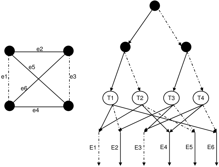
Figure 5. The main building block for the reduction.

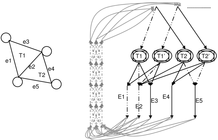
Figure 6. The complete reduction.

We have shown in Section 3 how to check in polynomial time if a colored graph is partly observable. Hence the problem is in P and to complete the proof it suffices to exhibit a polynomial time reduction from some NP-complete problem. Our proof proceeds by reduction from MONOCHROMATIC-TRIANGLE. In MONOCHROMATIC-TRIANGLE we are given an undirected graph $G$ and we are asked to assign one of two possible colors to every edge of $G$ so that no triangle in $G$ (a triangle in a graph is a clique of size three) has its three edges identically colored. A graph for which this is possible is said to be triangle-colorable and the problem of determining if a given graph is triangle-colorable is known to be NP-complete [4].

Our proof proceeds as follows: From an undirected graph $G$ we construct a directed graph $\tilde{G}$ that can be made partly observable with two colors if and only if $G$ is triangle-colorable. Thus we prove the somewhat stronger result that the problem of determining if a graph can be made partly observable with two colors, is NP-complete.

As is often the case for NP-hardness proofs the idea of the reduction is simple but the construction of the reduction is somewhat involved. For clarity we construct $\tilde{G}$ in two steps. The first step is illustrated on Figure 5. In this first step we construct an acyclic graph $G^{\prime}$ that will be used in the second step. The encoding of MONOCHROMATIC-TRIANGLE is done at this step. The second step is illustrated on Figure 6 and uses several replica of parts of the construction given in the first step. This second step is needed in order to make the final graph $\tilde{G}$ connected.

Let us now consider the first step. The left hand side of Figure 5 represents an undirected graph $G$. The edges of $G$ are colored but we do not pay attention to the colors at this stage. At the right hand side of the figure is the graph $G^{\prime}$ constructed from $G$. In order to construct $G^{\prime}$, we order the edges of $G$ and for every edge $e_{i}$ in $G$ we define two nodes in $G^{\prime}$ and a directed edge $E_{i}$ between them; these edges have no nodes in common and we refer to them as “real edges” because they represent edges in the original graph $G$. Next, we identify the triangles $\{e_{q},e_{r},e_{s}:q<r<s\}$ in $G$, we order them (for example, according to the lexicographic order), we add a node $T_{i}$ in $G^{\prime}$ for every triangle in $G$, and we add in $G^{\prime}$ edges from the node $T_{i}$ to all three real edges it is composed of, as illustrated on the second level of the graph on Figure 5. Thus the out-degrees of the nodes $T_{i}$ are all equal to three. Finally, we construct a binary tree whose leaves are the nodes $T_{i}$. In the example represented on the figure, the graph $G$ has four triangles and so the tree has four leaves $T_{i}$ and has depth 2. (In general, the tree has depth equal to $N=\lceil\log_{2}{S}\rceil$ where $S$ is the number of triangles in $G$.) The reduction will be based on the following observation: Let the edges of $G^{\prime}$ be colored and let us consider the sequences of colors observed on paths from the root of the tree to the bottom nodes. We claim that the edges of $G^{\prime}$ can be colored with two colors so that all color sequences observed on these paths are different if and only if $G$ can be triangle-colored. We now establish this claim. Assume first that $G$ can not be triangle-colored and let $T_{i}$ be a node corresponding to a triangle whose edges are identically colored. There are three outgoing edges from $T_{i}$ and so two of them must have identical colors. Since these edges lead to real edges of identical colors, $G^{\prime}$ has two paths that have identical color sequences. Assume now that the graph $G$ can be triangle-colored. We color the real edges of $G^{\prime}$ with their corresponding colors in $G$ and we color the edges of the tree so that paths from root to leaves define different color sequences. It remains to color the outgoing edges from the nodes $T_{i}$. Every $T_{i}$ has three outgoing edges $u_{i},v_{i},w_{i}$ and these edges lead to real edges that are not all identically colored. Since there are only two colors, two of the three edges must have identical colors. Let $u_{i}$ and $v_{i}$ be the outgoing edges from $T_{i}$ that lead to the two identically colored real edges; we give to $u_{i}$ and $v_{i}$ different colors and choose an arbitrary color for the third outgoing edge $w_{i}$. When coloring the edges of $G^{\prime}$ in this way, all paths from the root to the bottom nodes define different color sequences and so the claim is established.

We now describe the second step of the construction. This step is illustrated on Figure 6 where we show a graph $G$ (on the left hand side) and the corresponding graph $\tilde{G}$ (on the right hand side) constructed from $G$. Notice that the graph $G$ we consider here is different from the graph used in Figure 5. The construction of $\tilde{G}$ consists in repeating a number of times the tree structure described in the first step and then making the graph connected by connecting the end nodes of the real edges to the roots of the trees through a sequence of edges, as represented on the figure. For the sake of clarity we have represented only two copies of the tree on the figure but the complete construction has $2S+1$ such copies (in the example of the figure, 5 copies); the reason for having $2S+1$ copies will appear in an argument given below. In the sequence of edges that make the graph connected there are three nodes at every level and there are $N+3$ levels where $N$ is the depth of the trees. The aim of this last construction is to make us able, by appropriately coloring the edges, to determine when an agent reaches the root of a tree, but without making us able to determine what particular root the agent has reached.

We are now able to conclude the proof. We want to establish that $\tilde{G}$ can be made partly observable with two colors iff $G$ is triangle-colorable.

Assume first that $G$ is triangle-colorable and let the coloration be given with the colors dashed (D) and Solid (S). We color $\tilde{G}$ as follows: For the real edges and for the edges in the trees we choose the colors described in step 1, for the edges leaving the end nodes of the real edges and for the incoming edges to the roots we choose S, finally, all the other connecting edges are colored by D. We claim that the graph $\tilde{G}$ so colored is partly observable. In order to establish our claim consider an agent moving in $\tilde{G}$. After some time the agent will hit a long sequence of $N+3$ connecting edges colored by D. The agent will know that he is at a root as soon as he observes a S. He will however not be able to determine what particular root he is at. We then use the argument presented in step 1 to conclude that, when the agent subsequently arrives at one of the end node of the real edges, he knows exactly at what node he is. Therefore the colored graph $\tilde{G}$ is partly observable because, whenever the agent reaches the end node of a real edge, he knows where he is.

We now establish the other direction: If $G$ is not triangle-colorable then $\tilde{G}$ cannot be made partly observable with two colors. We establish this by proving that when $G$ is not triangle-colorable, then there exist two separated cycles in $\tilde{G}$ that have identical color sequences. Since the color sequences are identical and the cycles are separated an agent observing that particular repeated color sequence can never determine on what cycle he is and the graph is not partly observable. Let us assume that some coloration for $\tilde{G}$ has been chosen. Since $G$ is not triangle-colorable, some triangles have all their edges identically colored. Choose one such triangle and consider in every tree in $\tilde{G}$ the path that leads from the root to the node corresponding to that triangle in the tree. Any such path defines a color sequence and there are at most $S$ such sequences. Since there are $2S+1\geq S+1$ trees, we may conclude by the pigeonhole principle that there are two separated but identically colored paths that leave from distinct roots and lead to leaves corresponding to the same triangle. If we require in addition that both roots have two incoming edges colored with the same color, then the same result applies since there are $2S+1$ trees. By using the definition of $\tilde{G}$ and the fact that $G$ cannot be triangle-colored, the construction of two identically colored distinct cycles can be continued by constructing paths from the two nodes corresponding to the uni-colored triangle to the roots of their corresponding trees. In this way one can construct two separated but identically colored cycles in $\tilde{G}$ that prove that $\tilde{G}$ cannot be made observable with two colors and the proof is complete.

∎

5. Conclusion and future work

We have introduced and analyzed a simple notion of observability in graphs. Observability in graphs is desirable in situations where autonomous agents move on a network and one want to localize them; this concept appears in a number of different areas. We have characterized various forms of observability and have shown how they can be checked in polynomial time. We have also shown that the time needed to localize an agent in a graph can be computed in polynomial time. This time is in the worst case quadratic in the number of nodes in the graph. We have also proved that the design of observable graphs is NP-complete in two distinct situations. We leave some open questions and problems: Is the problem of making a graph observable NP-complete if colors are assigned to the edges? How can one approximate the minimal number of colors? If a graph can be made observable with a certain number of colors, how can the colors be assigned so as to minimize the time necessary to localize the agent?

References

- [1] M.-P. Beal. Codage symbolique. Masson, 1993.
- [2] V. Crespi, G. V. Cybenko, and G. Jiang. The Theory of Trackability with Applications to Sensor Networks. Technical Report TR2005-555, Dartmouth College, Computer Science, Hanover, NH, August 2005.
- [3] Y. Ephraim and N. Merhav. Hidden markov processes. IEEE Transactions on Information Theory, 48(6):1518–1569, 2002.
- [4] M. R. Garey and D. S. Johnson. Computers and Intractability; A Guide to the Theory of NP-Completeness. W. H. Freeman & Co., New York, NY, USA, 1990.
- [5] R. Jungers, V. Protasov, and V.D. Blondel. Efficient algorithms for deciding the type of growth of products of integer matrices. submitted to publication.
- [6] C. M. Özveren and A.S. Willsky. Observability of discrete event dynamic systems. IEEE Transactions on automatic and control, 35:797–806, 1990.
- [7] L. R. Rabiner. A tutorial on hidden markov models and selected apllications in speech recognition. In A. Waibel and K.-F. Lee, editors, Readings in Speech Recognition, pages 267–296. Kaufmann, San Mateo, CA, 1990.
- [8] A. J. Viterbi. Error bounds for convolutional codes and an asymptotically optimal decoding algorithm. IEEE Transaction on Information Theory, IT-13:260–269, 1967.