Paths Beyond Local Search: A Nearly Tight Bound
for Randomized Fixed-Point Computation

Abstract

In 1983, Aldous proved that randomization can speedup local search. For example, it reduces the query complexity of local search over $[1:n]^{d}$ from $\Theta(n^{d-1})$ to $O(d^{1/2}n^{d/2})$. It remains open whether randomization helps fixed-point computation. Inspired by this open problem and recent advances on equilibrium computation, we have been fascinated by the following question:

Is a fixed-point or an equilibrium fundamentally harder to find than a local optimum?

In this paper, we give a nearly-tight bound of $\left(\Omega\left(n\right)\right)^{d-1}$ on the randomized query complexity for computing a fixed point of a discrete Brouwer function over $[1:n]^{d}$. Since the randomized query complexity of global optimization over $[1:n]^{d}$ is $\Theta(n^{d})$, the randomized query model over $[1:n]^{d}$ strictly separates these three important search problems:

Global optimization is harder than fixed-point computation, and
fixed-point computation is harder than local search.

Our result indeed demonstrates that randomization does not help much in fixed-point computation in the query model; the deterministic complexity of this problem is $\Theta(n^{d-1})$.

Prologue

• On the first day of your new job, your boss teaches you the Simplex Algorithm with the Steepest-Edge Pivoting Rule. You quickly master the steps of the algorithm. So she gives you a large linear program that simulates a new business model.

  “I am going to a convention in Hawaii for ten days. Could you work on the program starting with this initial vector $\mathbf{x}_{0}$?” she asks. “The solution will be a vector that you cannot improve upon. Email it to me when you are done”

  So she leaves for beautiful Hawaii and you begin your iterative path-following search. Ten days later, she comes back, relaxed, right as you finish computing $\mathbf{x}_{1000000}$!

  “I haven’t found the solution yet,” you report, “but I have followed the steepest-edges a million steps and get $\mathbf{x}_{1000000}$.”

  She takes the objective vector $\mathbf{c}$ and quickly computes $\mathbf{c}^{T}\mathbf{x}_{1000000}/\mathbf{c}^{T}\mathbf{x}_{0}$, and it is $1.10$.

  “You find a vector that is 10 percent better than what we had initially,” she says cheerfully. “Good job!”

  The next day, you get a ten-percent raise.

• On the first day of your new job, your boss teaches you the Lemke-Howson algorithm for finding a Nash equilibrium of a two-player game. You quickly master the steps of the algorithm. So he gives you a large two-player game that models a two-group exchange market.

  “I am going to a convention in Hawaii for ten days. Could you work on this two-player game?” he asks. “Here is an initial strategy-profile,” he gives you $(\mathbf{x}_{0},\mathbf{y}_{0})$, “and the strategy-profile that Lemke-Howson halts on is a Nash equilibrium. Email it to me when you are done.”

  So he leaves for beautiful Hawaii and you begin your iterative path-following search. Ten days later, he comes back, relaxed, right as you finish computing $(\mathbf{x}_{1000000},\mathbf{y}_{1000000})$!

  “I haven’t found the solution yet,” you report, “but I have followed the Lemke-Howson path a million steps and get $(\mathbf{x}_{1000000},\mathbf{y}_{1000000})$.”

  He looks at $(\mathbf{x}_{1000000},\mathbf{y}_{1000000})$ for a while and then frowns, just slightly.

  “Hmmmm, no equilibrium in a million steps!” he says. “Well, good job and thanks.”

  The next day, you still have your job but get no raise.

1 Introduction

The Simplex Algorithm [11] is an example of an implementation of local search and finding a Nash equilibrium [22] is an example of fixed-point computation (FPC). A general approach for local search is Iterative Improvement. Steepest-Descent is its most popular example. It follows a path in the feasible space, a path along which the objective values are monotonically improving. The end of the path is a local optimum. Like Iterative Improvement, many algorithms for FPC, such as the Lemke-Howson algorithm [20] and the constructive proof of Sperner’s Lemma [29], also follow a path whose endpoint is an equilibrium or a fixed-point. But unlike a path in local search, a path in FPC does not have an obvious “locally computable” monotonic measure-of-progress. Moreover, path following in FPC from an arbitrary point could lead to a cycle while the union of paths in Iterative Improvement is acyclic.

Do these structural differences have any algorithmic implication?

There have been increasing evidence, beyond the stories of our prologue, that local search and FPC are very different. First, Aldous [2] showed that randomization can speedup local search (more discussion below). His method crucially utilizes the monotonicity discussed above. It remains open whether randomization helps FPC. Second, polynomial-time path-following-like algorithms have been developed for some non-trivial classes of local search problems. These algorithms include the interior-point algorithm for linear and convex programming [18, 23] and edge-insertion algorithms for geometric optimization [13]. However, popular fixed-point problems, such as the computation of a Nash or a market equilibrium [3] might be hard for polynomial time [12, 7, 10]. Other than those that can be solved by convex programming, we haven’t yet discovered a significantly non-trivial class of equilibrium problems that are solvable in polynomial-time. Third, an approximate local optimum for every PLS (Polynomial Local Search) problem can be found in fully-polynomial time [24]. In contrast, although a faster randomized algorithm was found for approximating Nash equilibria [21], finding an approximate Nash equilibrium in fully-polynomial time is computationally equivalent to finding an exact Nash equilibrium in polynomial time [8]. We face the same challenge in approximating market equilibria [16]. Fourth, although they all have exponential worst-case complexity [27, 19], the smoothed complexity of the Simplex Algorithm and Lemke-Howson Algorithm (or Scarf’s market equilibrium algorithm [28]) might be drastically different [30, 8, 16]. This evidence inspires us to ask:

Is fixed-point computation fundamentally harder than local search?

To investigate this question, we consider the complexity of these two search problems defined over $\mathbb{Z}^{d}_{n}=[1:n]^{d}$. For fixed-points, we are given a function $F:\mathbb{Z}^{d}_{n}\rightarrow\mathbb{Z}^{d}_{n}$ that satisfies Brouwer’s condition [4] — a set of continuity and boundary conditions (see Section 2) — that guarantees the existence of a fixed-point. Recall that a vector $\mathbf{v}\in\mathbb{Z}^{d}_{n}$ is a fixed-point of $F$ if $F(\mathbf{v})=\mathbf{v}$. The FPC problem is to find a fixed-point of $F$. For local optima, we are given a function $h:\mathbb{Z}^{d}_{n}\rightarrow\mathbb{R}$. The local search problem is to find a local optimum of $h$, for example, a vector $\mathbf{x}\in\mathbb{Z}^{d}_{n}$ such that $h(\mathbf{x})\geq h(\mathbf{y})$, $\forall\mathbf{y}$ with $||\mathbf{x}-\mathbf{y}||_{1}\leq 1$.

For both problems, we consider the query complexity in the query model: The algorithm can only access $F$ and $h$, respectively, by asking queries of the form: “What is $F(\mathbf{x})$?” and “What is $h(\mathbf{x})$?”. The complexity is measured by the number of queries needed to find a solution.

There are some similarities between FPC and local search over $\mathbb{Z}^{d}_{n}$. For both, divide-and-conquer has positive but limited success: Both problems can be solved by $O(n^{d-1})$ queries [5]. An alternative approach to solve both problems is path-following. When following a short path, it can be faster than divide-and-conquer. But for both problems, long and winding paths are the cause of inefficiency.

However, there is one prominent difference between a path to a local optimum and a path to a fixed point. The values of $h$ along a path to a local optimum are monotonic, serving as a measure-of-progress along the path. Aldous [2] used this fact in a randomized algorithm: Randomly query $d^{1/2}n^{d/2}$ points in $\mathbb{Z}^{d}_{n}$; let $\mathbf{s}$ be the sample point with the largest $h$ value; follow a path starting at $\mathbf{s}$. If a path to a local optimum is long, say much longer than $d^{1/2}n^{d/2}$, then with high probability, the random samples intersect the path and partition it into sub-paths, each with expected length $O(d^{1/2}n^{d/2})$. As $\mathbf{s}$ has the largest $h$ value, its sub-path is the last sub-path of a potentially long path, and we expect its length to be $O(d^{1/2}n^{d/2})$. So with randomization, Aldous reduced the expected query complexity to $O(d^{1/2}n^{d/2})$.

But it remains open whether randomization can reduce the query complexity of FPC over $\mathbb{Z}^{d}_{n}$. The lack of a measure-of-progress along a path makes it impossible for us to directly use Aldous’ idea.

Our Main Result

The state of our knowledge suggests that FPC might be significantly harder than local search, at least in the randomized query model. We have formulated a concrete conjecture stating that an expected number of $\left(\Omega\left(n\right)\right)^{d-1}$ queries are needed in randomized FPC over $\mathbb{Z}^{d}_{n}$.

As the main technical result of this paper, we prove that an expected number of $\left(\Omega\left(n\right)\right)^{d-1}$ queries are indeed needed. Our lower bound is essentially tight, since the deterministic divide-and-conquer algorithm in [5] can find a fixed point by querying $O(n^{d-1})$ vectors. In contrast to Aldous’s result [2], our result demonstrates that randomization does not help much in FPC in the query model. It shows that, in the randomized query model over $\mathbb{Z}^{d}_{n}$, a fixed-point is strictly harder to find than a local optimum! The significant gap between these two problems is revealed only in randomized computation. In the deterministic framework, both have query complexity $\Theta(n^{d-1})$.

One can show that the randomized query complexity for finding a global optimum over $\mathbb{Z}^{d}_{n}$ is $\Theta(n^{d})$. So, the randomized query model over $\mathbb{Z}^{d}_{n}$ strictly separates these three important search problems:

Global optimization is harder than fixed-point computation, and
fixed-point computation is harder than local search.

We anticipate that a similar gap can be obtained in the quantum query model.

Related Work and Technical Contributions

Our work is also inspired by the lower bound results of Aaronson [1], Santha and Szegedy [26], Zhang [33], and Sun and Yao [31] on the randomized and quantum query complexity of local search over $\mathbb{Z}^{d}_{n}$.

In this paper, we introduce several new techniques to study the complexity of FPC. Instrumental to our analysis, we develop a method to generate hard-to-find random long paths in the grid graph over $\mathbb{Z}^{d}_{n}$. To achieve our nearly-tight lower bound, these paths must be much longer than the random paths constructed in [33, 31] for local search. Our paths has expected length $\left(\Theta(n)\right)^{d-1}$ while those random paths for local search have length $\Theta(n^{d/2})$. We also develop new techniques for unknoting a self-intersecting path and for realizing a path with a Brouwer function. These techniques might be useful on their own in the future algorithmic and complexity-theoretic studies of FPC and its applications.

There are several earlier work on the query complexity of FPC. Hirsch, Papadimitriou and Vavasis [15] considered the deterministic query complexity of FPC. They proved a tight $\Theta(n)$ bound for ${\mathbb{Z}^{2}_{n}}$ and an $\Omega(n^{d-2})$ lower bound for $\mathbb{Z}^{d}_{n}$. Subsequently, Chen and Deng [5] improved this bound to $\Theta(n^{d-1})$ for $\mathbb{Z}^{d}_{n}$. Recently, Friedl, Ivanyos, Santha, and Verhoeven [14] gave a $\Omega(n^{1/4})$-lower bound on the randomized query-complexity of the 2D Sperner problem. Our method for unkonting self-intersecting paths can be viewed as an extension of the 2D technique of [6] to high dimensions.

Paper Organization

In Section 2, we introduce three high-dimensional search problems. In Section 3, we reduce one of them, called End-of-a-String, to fixed-point computation over $\mathbb{Z}^{d}_{n}$. In Section 4, we give a nearly tight bound on the randomized query complexity of End-of-a-String. Together with the reduction in Section 3, we obtain our main result on fixed-point computation.

2 Three High-Dimensional Search Problems

We will define three search problems. The first one concerns FPC. We introduce the last two to help the study of the first one. Below, let $\mathbb{E}^{d}=\{\pm\mathbf{e}_{1},\pm\mathbf{e}_{2},...,\pm\mathbf{e}_{d}\}$ be the set of principle unit-vectors in $d$-dimensions. Let $\|\cdot\|$ denote $\|\cdot\|_{\infty}$. For two vectors $\mathbf{u}\not=\mathbf{v}$ in $\mathbb{Z}^{d}$, we say $\mathbf{u}<\mathbf{v}$ lexicographically if $u_{i}<v_{i}$ and $u_{j}=v_{j}$ for all $1\leq j<i$, for some $i$.

For each of the three search problems, we will define its mathematical structure, a query model for accessing this structure, the search problem itself, and its query complexity.

2.1 Discrete Brouwer Fixed-Points

Recall that a vector $\mathbf{v}\in\mathbb{Z}^{d}_{n}$ is a fixed-point of a function $F$ from $\mathbb{Z}^{d}_{n}$ to $\mathbb{Z}^{d}_{n}$ if $F(\mathbf{v})=\mathbf{v}$. A function $f:\mathbb{Z}^{d}_{n}\rightarrow\{\mathbf{0}\}\cup\mathbb{E}^{d}$ is bounded if $f(\mathbf{x})+\mathbf{x}\in\mathbb{Z}^{d}_{n}$ for all $\mathbf{x}\in\mathbb{Z}^{d}_{n}$; $\mathbf{v}\in\mathbb{Z}^{d}_{n}$ is a zero point of $f$ if $f(\mathbf{v})=\mathbf{0}$. Clearly, if $F(\mathbf{x})=\mathbf{x}+f(\mathbf{x})$ for all $\mathbf{x}\in\mathbb{Z}^{d}_{n}$, then $\mathbf{v}$ is a fixed point of $F$ iff $\mathbf{v}$ is a zero point of $f$.

Definition 2.1 (Direction Preserving Functions).

A function $f$ from $S$ to $\{\hskip 0.85355pt\mathbf{0}\hskip 0.85355pt\}\cup\mathbb{E}^{d}$ where $S\subset\mathbb{Z}^{d}$ is direction-preserving if $\|f(\mathbf{r}_{1})-f(\mathbf{r}_{2})\|\leq 1$ for all pairs $\mathbf{r}_{1},\mathbf{r}_{2}\in S$ such that $\|\mathbf{r}_{1}-\mathbf{r}_{2}\|\leq 1$.

Following the discrete fixed-point theorem of [17], we have: For every function $f:\mathbb{Z}^{d}_{n}\rightarrow\{\mathbf{0}\}\cup\mathbb{E}^{d}$, if $f$ is both bounded and direction-preserving, then there exists $\mathbf{v}\in\mathbb{Z}^{d}_{n}$ such that $f(\mathbf{v})=\mathbf{0}$. We refer to a bounded and direction-preserving function $f$ over $\mathbb{Z}^{d}_{n}$ as a Discrete Brouwer function or simply a Brouwer function over $\mathbb{Z}^{d}_{n}$. In the query model, one can only access $f$ by asking queries of the form: “What is $f(\mathbf{r})$?” for a query point $\mathbf{r}\in\mathbb{Z}^{d}_{n}$.

The FPC problem $\text{\sf ZP}^{d}$ that we will study is as follows: Given a Brouwer function $f$ from $\mathbb{Z}^{d}_{n}$ to $\{\mathbf{0}\}\cup\mathbb{E}^{d}$ in the query model, find a zero point of $f$. Let $\text{\sf RQ}_{\text{\sf ZP}}(f)$ denote the expected number of queries needed by the best randomized algorithm to find a zero point of $f$. We let

$$\text{\sf RQ}_{\text{\sf ZP}}^{d}(n)=\max_{f:\ \text{Brouwer function over $\mathbb{Z}^{d}_{n}$}}\big{\{}\hskip 1.13791pt\text{\sf RQ}_{\text{\sf ZP}}(f)\hskip 1.13791pt\big{\}},\vspace{-0.1cm}$$

be the randomized query complexity for solving $\text{\sf ZP}^{d}$. In this paper, we will prove:

Theorem 2.2 (Randomized Query Complexity of Fixed Points).

There is a constant $c$ such that for all sufficiently large $n$,

$$\text{\sf RQ}_{\text{\sf ZP}}^{d}(n)\geq\left(\frac{n}{c^{d}}\right)^{d-1}.$$

In contrast, the deterministic query complexity for solving $\text{\sf ZP}^{d}$ is at most $7n^{d-1}$ [5]. The Brouwer fixed point problem defined here is computationally equivalent to the fixed problems defined in [15, 12, 8]. Thus, our result carries over to these FPC problems.

2.2 End-of-a-Path in Grid-PPAD Graphs

The mathematical structure for this search problem is a directed graph $G=(V,E)$. A vertex $v\in V$ satisfies Euler’s condition if $\Delta_{I}(v)=\Delta_{O}(v)$ where $\Delta_{I}(v)$ and $\Delta_{O}(v)$ are the in-degree and the out-degree of $v$. We start with the following definition motivated by Papadimitriou’s PPAD class [25].

Definition 2.3 (Generalized PPAD Graphs).

A directed graph $G=(V,E)$ is a generalized PPAD graph if (1) there exists exactly one vertex $v_{S}\in V$ with $\Delta_{O}(v_{S})=\Delta_{I}(v_{S})+1$ and exactly one vertex $v_{T}\in V$ with $\Delta_{I}(v_{T})=\Delta_{O}(v_{T})+1$. (2) all vertices in $V-\{\hskip 0.56917ptv_{S},v_{T}\hskip 0.56917pt\}$ satisfy Euler’s condition and (3) if $(v_{1},v_{2})$ is a directed edge in $E$, then $(v_{2},v_{1})\not\in E$. We refer to $v_{S}$ and $v_{T}$ as the starting and ending vertices of $G$, respectively.

We call $G$ a PPAD graph if in addition $\Delta_{I}(v),\Delta_{O}(v)\leq 1$, for all $\ v\in V$.

Edges of a PPAD graph form a collection of disjoint directed cycles and a directed path from $v_{S}$ to $v_{T}$. In this paper, we are interested in a special family of PPAD graphs over $\mathbb{Z}^{d}_{n}$. A directed graph $G=(\mathbb{Z}_{n}^{d},E)$ is a generalized grid PPAD-graph over $\mathbb{Z}_{n}^{d}$ if it is a generalized PPAD graph and the underlying undirected graph of $G$ is a subgraph of the grid graph defined over $\mathbb{Z}^{d}_{n}$. Moreover, if $G$ is also a PPAD graph, then we say $G$ is a grid PPAD graph.

We now define the query model $\mathbb{B}_{G}$ for accessing a grid PPAD graph $G$.

Definition 2.4 ($\mathbb{B}_{G}$).

$\mathbb{B}_{G}$ is a map from $\mathbb{Z}^{d}_{n}$ to $(\{\text{``no''}\}\cup\mathbb{E}^{d})\times(\{\text{``no''}\}\cup\mathbb{E}^{d})$ such that, for all $\mathbf{v}\in\mathbb{Z}^{d}_{n}$,

• $\mathbb{B}_{G}(\mathbf{v})=(\text{``no''},\mathbf{v}_{1}-\mathbf{v})$ if $\mathbf{v}$ is the starting vertex of $G$ and $(\mathbf{v},\mathbf{v}_{1})\in E$;

• $\mathbb{B}_{G}(\mathbf{v})=(\mathbf{v}-\mathbf{v}_{1},\text{``no''})$ if $\mathbf{v}$ is the ending vertex of $G$ and $(\mathbf{v}_{1},\mathbf{v})\in E$;

• $\mathbb{B}_{G}(\mathbf{v})=(\mathbf{v}-\mathbf{v}_{1},\mathbf{v}_{2}-\mathbf{v})$ if $(\mathbf{v}_{1},\mathbf{v})$ and $(\mathbf{v},\mathbf{v}_{2})$ are directed edges of $G$.

• $\mathbb{B}_{G}(\mathbf{v})=(\text{``no''},\text{``no''})$, otherwise.

In other words, $\mathbb{B}_{G}$ specifies the predecessor and successor of each vertex $\mathbf{v}$ in $G$. We will use the property that if $\mathbb{B}_{G}(\mathbf{v})=(\mathbf{s}_{1},\mathbf{s}_{2})$ and $\mathbf{s}_{1},\mathbf{s}_{2}\in\mathbb{E}^{d}$, then $\mathbf{s}_{1}+\mathbf{s}_{2}\not=0$.

Let $\text{\sf GP}^{d}$ be the search problem: Given a triple $(G,0^{n},\mathbf{u})$, where $G$ is a grid PPAD graph over $\mathbb{Z}^{d}_{n}$ accessible by $\mathbb{B}_{G}$ and $\mathbf{u}$ is the starting vertex of graph $G$ satisfying $u_{d}=1$, find its ending vertex. We use $\text{\sf RQ}_{\text{\sf GP}}^{d}(n)$ to denote the randomized query complexity for solving this problem.

2.3 End-of-a-String

Suppose $\Sigma$ is a finite set. A string $S$ over $\Sigma$ of length $m$ is a sequence $S=a_{1}a_{2}...a_{m-1}a_{m}$ with $a_{i}\in\Sigma$. We use $|S|=m$ to denote the length of $S$.

Definition 2.5 (Non-Repeating-Strings).

A string $S=a_{1}a_{2}...a_{m}$ over $\mathbb{Z}_{n}=[1:n]$ is $d$-non-repeating for $d\in[1:m]$, if (1) each string over $\mathbb{Z}_{n}$ of length $d$ appears in $S$ at most once; (2) $a_{i}$ is odd if $i$ is a multiple of $d$ and $a_{i}$ is even otherwise; and (3) $m$ is a multiple of $d$. We define $\mbox{{\sf end}}_{d}\left(S\right)=a_{m-d+1}...a_{m}$.

Each $d$-non-repeating string $S=a_{1}...a_{m}$ over $\mathbb{Z}_{n}$ defines a query oracle $\mathbb{B}_{S}$ from $\mathbb{Z}_{n}^{d}$ to $(\{\text{``no''}\}\cup\mathbb{Z}_{n})\times(\{\text{``no''}\}\cup\mathbb{Z}_{n})$: For $S^{\prime}=b_{1}b_{2}...b_{d}\in\mathbb{Z}_{n}^{d}$, if $S^{\prime}$ is not a substring of $S$, then $\mathbb{B}_{S}(S^{\prime})=(\text{``no''},\text{``no''})$; otherwise, there is a unique $k$ such that $a_{k+i-1}=b_{i}$, $\forall\ i\in[1:d]$. Then $\mathbb{B}_{S}(S^{\prime})=(\text{``no''},a_{d+1})$ if $k=1$, $\mathbb{B}_{S}(S^{\prime})=(a_{m-d},\text{``no''})$ if $k=m-d+1$, i.e., $S^{\prime}=\mbox{{\sf end}}_{d}\left(S\right)$, and $\mathbb{B}_{S}(S^{\prime})=(a_{k-1},a_{k+d})$, otherwise.

Let $\text{\sf ES}^{d}$ be the search problem: Given a $d$-non-repeating string $S$ over $\mathbb{Z}_{n}$ accessible by $\mathbb{B}_{S}$, and its first $d$ symbols $a_{1}a_{2}...a_{d}$ where $a_{d}=1$, find $\mbox{{\sf end}}_{d}\left(S\right)$. We let $\text{\sf RQ}_{\text{\sf ES}}^{d}(n)$ denote its randomized query complexity. It is easy to show that $\text{\sf RQ}_{\text{\sf ES}}^{1}(n)=\Theta(n)$. In section 4, we will prove

Theorem 2.6 (Complexity of $\text{\sf ES}^{d}$).

For all sufficiently large $n$,

$$\text{\sf RQ}_{\text{\sf ES}}^{d}(4n+4)\hskip 1.70709pt\geq\frac{1}{2}\hskip 1.70709pt\hskip 1.70709pt\left(\hskip 0.85355pt\frac{n}{2\cdot 24^{d}}\hskip 0.85355pt\right)^{d}.\vspace{0.15cm}$$

3 Reduction Among Search Problems

In this section, we reduce $\text{\sf ES}^{d-1}$ to $\text{\sf ZP}^{d}$ by first reducing $\text{\sf ES}^{d-1}$ to $\text{\sf GP}^{d}$ (Theorem 3.1 below) and then reducing $\text{\sf GP}^{d}$ to $\text{\sf ZP}^{d}$ (Theorem 3.2). Theorem 2.2 then follows from Theorem 2.6.

Theorem 3.1 (From $\text{\sf ES}^{d-1}$ to $\text{\sf GP}^{d}$).

For all $d\geq 2$, $\text{\sf RQ}_{\text{\sf ES}}^{d-1}(n)\leq 4d\cdot\text{\sf RQ}_{\text{\sf GP}}^{d}(8n+1)$.

Theorem 3.2 (From $\text{\sf GP}^{d}$ to $\text{\sf ZP}^{d}$).

For all $d\geq 1$, $\text{\sf RQ}_{\text{\sf GP}}^{d}(n)\leq\text{\sf RQ}_{\text{\sf ZP}}^{d}(24n+7)$.

3.1 From $\text{\sf ES}^{d-1}$ to $\text{\sf GP}^{d}$: Proof of Theorem 3.1

Proof.

[of Theorem 3.1]: We define a map $\mathcal{F}_{d}$ from $\mathbb{Z}^{d-1}$ to $\mathbb{Z}^{d}$: for $d=2$, $\mathcal{F}_{2}(a)=(a,a)$; and for $d>2$, $\mathcal{F}_{d}(\mathbf{a})=(a_{1},a_{1}+a_{2},...,a_{d-2}+a_{d-1},a_{d-1})$. We will crucially use the following nice property of $\mathcal{F}_{d}$.

For any $k\in[1:d]$ and for any $\mathbf{a}\in\mathbb{Z}^{d-1}$, we can uniquely determine the first $k$ and
the last $k$ entries of $\mathbf{a}$, respectively, from the first $k$ and the last $k$ entries of $\mathcal{F}_{d}(\mathbf{a})$.

Let $S$ be a $(d-1)$-non-repeating string over $\mathbb{Z}_{n}$ of length $m(d-1)$ for some $m\geq 2$, whose $(d-1)^{st}$ symbol is $1$. We view $S$ as a sequence of $m$ points $\mathbf{a}_{1},\mathbf{a}_{2},...\mathbf{a}_{m}$ in $\mathbb{Z}_{n}^{d-1}$, where $\mathbf{a}_{i}=a_{i,1}...a_{i,d-1}$, such that, $S=a_{1,1}a_{1,2}...a_{1,d-1}...a_{m,1}a_{m,2}...a_{m,d-1}.$ From $S$, we will construct a grid PPAD graph $G^{\prime}$ in two stages. In the first stage, we construct a generalized grid PPAD graph $G^{*}$ over $\mathbb{Z}_{2n}^{d}$ such that

  (A.1)

Its starting vertex is $\mathbf{u}^{*}=\mathcal{F}_{d}(\mathbf{a}_{1})$ and its ending vertex is $\mathbf{w}^{*}=\mathcal{F}_{d}(\mathbf{a}_{m})$;

  (A.2)

For every directed edge $(\mathbf{u},\mathbf{v})$ with $\mathbf{u}-\mathbf{v}\in\mathbb{E}^{d}$, at most one query to $\mathbb{B}_{S}$ is needed to determine whether $(\mathbf{u},\mathbf{v})\in G^{*}$.

Recall that a directed path is simple if it contains each vertex at most once. Suppose $\mathbf{u},\mathbf{v}\in\mathbb{Z}_{2n}^{d}$ are two vertices that differ in only one coordinate, say the $i^{th}$ coordinate. Suppose $\mathbf{e}=(\mathbf{v}-\mathbf{u})/|v_{i}-u_{i}|\in\mathbb{E}^{d}$. Let $E(\mathbf{u},\mathbf{v})=\left\{(\mathbf{u},\mathbf{u}+\mathbf{e}),(\mathbf{u}+\mathbf{e},\mathbf{u}+2\mathbf{e}),...,(\mathbf{v}-\mathbf{e},\mathbf{v})\right\}$. For $n,m_{1},m_{2}\in\mathbb{Z}$ and $s\in\{\hskip 1.13791pt\pm 1\hskip 1.13791pt\}$, $(n,s)$ is consistent with $(m_{1},m_{2})$ if either $m_{1}\leq n<m_{2}$ and $s=+1$ or $m_{2}<n\leq m_{1}$ and $s=-1$.

We consider two consecutive points $\mathbf{a}=\mathbf{a}_{t}$ and $\mathbf{b}=\mathbf{a}_{t+1}$ in the $(d-1)$-non-repeating string $S$. We know $\mathbf{a}\not=\mathbf{b}$. We map them to vertices $\mathbf{u}=\mathcal{F}_{d}(\mathbf{a})$ and $\mathbf{w}=\mathcal{F}_{d}(\mathbf{b})$ in $\mathbb{Z}_{2n}^{d}$ and connect them with a path through a sequence of $(d-1)$ vertices $\mathbf{v}_{0}=\mathbf{u},\mathbf{v}_{1},...,\mathbf{v}_{d-1},\mathbf{v}_{d}=\mathbf{w}$ where $v_{i,j}=u_{j}$ if $i<j$ and $v_{i,j}=w_{j}$ if $i\geq j$. Note that $\mathbf{v}_{i-1}$ and $\mathbf{v}_{i}$ differ only in the $i^{th}$ coordinate. Let $P(\mathbf{a},\mathbf{b})=\cup_{i=0}^{d-1}E\left(\mathbf{v}_{i},\mathbf{v}_{i+1}\right)$. Then $P(\mathbf{a},\mathbf{b})$ is a simple directed path in the grid graph over $\mathbb{Z}_{2n}^{d}$ from $\mathbf{u}=\mathbf{v}_{0}$ to $\mathbf{w}=\mathbf{v}_{d}$. As $S$ is $(d-1)$-non-repeating, $\mathbf{a}_{1}\not=\mathbf{a}_{m}$. By Property 3.3, Proposition 3.4 and Lemma 3.5 below, $G^{*}=(\mathbb{Z}^{d}_{2n},\cup_{i=1}^{m-1}P(\mathbf{a}_{i},\mathbf{a}_{i+1}))$ is a generalized grid PPAD graph. See Figure 1 for an example.

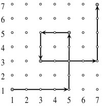
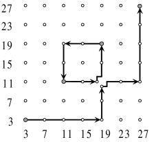
Figure 1: Graph $G^{*}$ and $G^{\prime}$ constructed from string $1537$

Proposition 3.3 (Path Union).

Let $P_{1},P_{2},...,P_{m}$ be $m$ simple directed paths over $V$ such that (1) each path has length at least one, (2) the ending vertex of $P_{i}$ is same as the starting vertex of $P_{i+1}$, (3) the starting vertex of $P_{1}$ is different from the ending vertex of $P_{m}$, and (4) if $(u,v)\in P_{i}$, then $(u,v),(v,u)\notin P_{j}$, $\forall j\not=i$. Then $G=(V,\cup_{i=1}^{m}P_{i})$ is a generalized PPAD graph.

Proposition 3.4 (Local Characterization of $P(\mathbf{a},\mathbf{b})$).

For $\mathbf{v}\in\mathbb{Z}_{2n}^{d}$ and $s\in\{\pm 1\}$,

1. $(\mathbf{v},\mathbf{v}+s\mathbf{e}_{1})\in P(\mathbf{a},\mathbf{b})$ if and only if $(v_{1},s)$ is consistent with $(a_{1},b_{1})$, $a_{d-1}=v_{d}$, and $a_{d-i}=v_{d-i+1}-a_{d-i+1}$ for all $2\leq i\leq d-1$;

2. $(\mathbf{v},\mathbf{v}+s\mathbf{e}_{d})\in P(\mathbf{a},\mathbf{b})$ if and only if $(v_{d},s)$ is consistent with $(a_{d-1},b_{d-1})$, $b_{1}=v_{1}$, and $b_{i}=v_{i}-b_{i-1}$, for $2\leq i\leq d-1$; and

3. for $1<k<d$, $(\mathbf{v},\mathbf{v}+s\mathbf{e}_{k})\in P(\mathbf{a},\mathbf{b})$ if and only if $(v_{k},s)$ is consistent with $(a_{k-1}+a_{k},b_{k-1}+b_{k})$ and (3.1) $a_{d-1}=v_{d}$, and $a_{d-i}=v_{d-i+1}-a_{d-i+1}$ for $2\leq i\leq d-k$ and (3.2) $b_{1}=v_{1}$, and $b_{i}=v_{i}-b_{i-1}$ for $2\leq i\leq k-1$.

Lemma 3.5 (Structural Correctness).

For all $(d-1)$-non-repeating string $S=\mathbf{a}_{1}\mathbf{a}_{2}...\mathbf{a}_{m}$ over $\mathbb{Z}_{n}$, if $(\mathbf{u},\mathbf{v})\in P(\mathbf{a}_{i},\mathbf{a}_{i+1})$ then $(\mathbf{u},\mathbf{v}),(\mathbf{v},\mathbf{u})\notin P(\mathbf{a}_{j},\mathbf{a}_{j+1})$ for all $i\neq j$.

Proof.

We only prove the case when $\mathbf{e}=\mathbf{v}-\mathbf{u}=s\mathbf{e}_{k}$ with $1<k<d$ and $s\in\{\pm 1\}$. The other two cases are similar. From Proposition 3.4, $(\mathbf{u},\mathbf{v})\in P(\mathbf{a}_{i},\mathbf{a}_{i+1})$ implies that $\mathbf{a}_{i}$ and $\mathbf{a}_{i+1}$ satisfy conditions (3.1) and (3.2). If $(\mathbf{u},\mathbf{v})$ or $(\mathbf{v},\mathbf{u})$ is in $P(\mathbf{a}_{j},\mathbf{a}_{j+1})$, then $\mathbf{a}_{j}$ and $\mathbf{a}_{j+1}$ also satisfy these two conditions. Then $a_{i,k}a_{i,k+1}...a_{i,d-1}a_{i+1,1}...a_{i+1,k-1}=a_{j,k}a_{j,k+1}...a_{j,d-1}a_{j+1,1}...a_{j+1,k-1},$ which contradicts with the assumption that $S$ is $(d-1)$-non-repeating. ∎

We prove Property A.2 as follows.

Proof of Property A.2.

We will only prove for the case when $\mathbf{e}=\mathbf{v}-\mathbf{u}=s\mathbf{e}_{k}$ with $1<k$ $<d$. The other two cases are similar and simpler. To determine whether $(\mathbf{u},\mathbf{v})\in G^{*}$ or not, we consider the string $S^{\prime}=a_{k}a_{k+1}...a_{d-1}b_{1}...b_{k-1}$ that satisfies both (3.1) and (3.2) in Proposition 3.4. Edge $(\mathbf{u},\mathbf{v})\in G^{*}$ if and only if 1) $S^{\prime}\in\mathbb{Z}^{d-1}_{n}$; 2) $a_{d-1}$ is odd; 3) $\mathbb{B}_{S}(S^{\prime})=(a,b)$ for some $a,b\in\mathbb{Z}_{n}$; and 4) $(u_{k},s)$ is consistent with $(a+a_{k},b_{k-1}+b)$, So, only one query to $\mathbb{B}_{S}$ is needed. ∎

In the second stage, we construct a grid PPAD graph $G^{\prime}$ over $\mathbb{Z}^{d}_{8n+1}$ from graph $G^{*}$. Let $\Gamma(\mathbf{v})=4\mathbf{v}-\mathbf{1}$ for all $\mathbf{v}\in\mathbb{Z}_{2n}^{d}$. Our $G^{\prime}$ will satisfy the following two properties. See Figure 1 for an example.

  (B.1)

Its starting vertex is $\mathbf{u}^{\prime}=\Gamma(\mathbf{u}^{*})-2\mathbf{e}_{d}$; its ending vertex $\mathbf{w}^{\prime}$ satisfies $\|\mathbf{w}^{\prime}-\Gamma(\mathbf{w}^{*})\|\leq 1$;

  (B.2)

For each $\mathbf{v}\in\mathbb{Z}^{d}_{8n+1}$, one can determine $\mathbb{B}_{G^{\prime}}(\mathbf{v})$ from the predecessors and successors of $\mathbf{u}$ in $G^{*}$, where $\mathbf{u}$ is the lexicographically smallest vertex such that $\|\mathbf{v}-\Gamma(\mathbf{u})\leq 2\|$.

Two subsets $H_{1}$ and $H_{2}$ of $\mathbb{E}^{d}$, where $d\geq 2$, form a balanced-non-canceling pair if $|H_{1}|=|H_{2}|$ and $\mathbf{s}_{1}+\mathbf{s}_{2}\not=\mathbf{0}$ for all $\mathbf{s}_{1}\in H_{1}$ and $\mathbf{s}_{2}\in H_{2}$. Let $H_{I}(\mathbf{u})=\{\hskip 1.13791pt\mathbf{e}\in\mathbb{E}^{d}\ |\ (\mathbf{u}-\mathbf{e},\mathbf{u})\in E^{*}\hskip 1.13791pt\}$ be the vector differences of $\mathbf{u}$ and its predecessors in $G^{*}$. Similarly, let $H_{O}(\mathbf{u})=\{\hskip 1.13791pt\mathbf{e}\in\mathbb{E}^{d}\ |\ (\mathbf{u},\mathbf{u}+\mathbf{e})\in E^{*}\hskip 1.13791pt\}$ be the vector differences of the successors of $\mathbf{u}$ and $\mathbf{u}$. In the construction below, we will use the fact that if $\mathbf{u}$ satisfies Euler’s condition then $(H_{I},H_{O})$ is a balanced-non-canceling pair.

Using the procedure of Figure 2, we build a graph $G[H_{1},H_{2}]=(\{\hskip 0.56917pt-1,0,+1\hskip 0.56917pt\}^{d},E[H_{1},H_{2}])$ for each balanced-non-canceling pair $H_{1}$ and $H_{2}$. $G[H_{1},H_{2}]$ has the following properties: (1) For every $\mathbf{u}\in\left\{{-1,0,+1}\right\}^{d}$, $\Delta_{I}(\mathbf{u}),\Delta_{O}(\mathbf{u})\leq 1$; (2) A vector $\mathbf{u}\in\left\{{-1,0,+1}\right\}^{d}$ has $\Delta_{I}(\mathbf{u})=0$ and $\Delta_{O}(\mathbf{u})=1$ iff there exists an $\mathbf{e}\in H_{1}$ such that $\mathbf{u}=\mathbf{0}-\mathbf{e}$; (3) A vector $\mathbf{u}\in\left\{{-1,0,+1}\right\}^{d}$ has $\Delta_{I}(\mathbf{u})=1$ and $\Delta_{O}(\mathbf{u})=0$ iff there exists an $\mathbf{e}\in H_{2}$ such that $\mathbf{u}=\mathbf{0}+\mathbf{e}$.

 

Graph $G[H_{1},H_{2}]$, where $(H_{1},H_{2})$ is a balanced-non-canceling pair

 

1 :	set edge set $E[H_{1},H_{2}]=\emptyset$
2 :	while $H_{1}\not=\emptyset$ do
3 :	let $\mathbf{s}_{1}$ be the smallest vector in $H_{1}$ and $\mathbf{s}_{2}$ be the largest vector in $H_{2}$
	according to the lexicographical ordering;
4 :	set $H_{1}=H_{1}-\{\hskip 0.85355pt\mathbf{s}_{1}\hskip 0.85355pt\}$ and $H_{2}=H_{2}-\{\hskip 0.85355pt\mathbf{s}_{2}\hskip 0.85355pt\}$;
5 :	set $E[H_{1},H_{2}]=E[H_{1},H_{2}]\cup\{\hskip 0.85355pt(\mathbf{0}-\mathbf{s}_{1},\mathbf{0}-\mathbf{s}_{1}+\mathbf{s}_{2}),(\mathbf{0}-\mathbf{s}_{1}+\mathbf{s}_{2},\mathbf{0}+\mathbf{s}_{2})\hskip 0.85355pt\}$

 

Figure 2: Construction of Graph $G[H_{1},H_{2}]=(\{-1,0,+1\}^{d},E[H_{1},H_{2}])$

Let $\mathbf{u}^{*}$ be the starting vertex and $\mathbf{w}^{*}$ be the ending vertex of $G^{*}$. We build a grid PPAD graph $G^{\prime}=(\mathbb{Z}_{8n+1}^{d},E^{\prime})$ by applying the procedure of Fig. 2 locally to every vertex $\mathbf{u}\in\mathbb{Z}_{2n}^{d}$ of $G^{*}$. We use $(H_{I}(\mathbf{u}),H_{O}(\mathbf{u}))$ or a slight modification of $(H_{I}(\mathbf{u}),H_{O}(\mathbf{u}))$ when $\mathbf{u}=\mathbf{u}^{*}$ or $\mathbf{w}^{*}$. Initially we set $E^{\prime}=\emptyset$. Recall $\Gamma(\mathbf{u})=4\mathbf{u}-\mathbf{1}$.

1. [ local embedding of the starting vertex ] Since $u^{*}_{d}=1$, we have $\mathbf{e}_{d}\notin H_{I}(\mathbf{u}^{*})$ and $-\mathbf{e}_{d}\notin H_{O}(\mathbf{u}^{*})$. Let $H_{I}=H_{I}(\mathbf{u}^{*})\cup\{\mathbf{e}_{d}\}$. We add edges $(\Gamma(\mathbf{u}^{*})-2\mathbf{e}_{d},\Gamma(\mathbf{u}^{*})-\mathbf{e}_{d})$ and $(\Gamma(\mathbf{u}^{*})+\mathbf{s}_{1},\Gamma(\mathbf{u}^{*})+\mathbf{s}_{2})$ to $E^{\prime}$ for all edges $(\mathbf{s}_{1},\mathbf{s}_{2})$ in $G[H_{I},H_{O}(\mathbf{u}^{*})]$.

2. [ local embedding of the ending vertex ] As $|H_{I}(\mathbf{w}^{*})|=|H_{O}(\mathbf{w}^{*})|+1$, $H_{I}(\mathbf{w}^{*})\not=\emptyset$. Let $\mathbf{e}$ be the smallest vector in $H_{I}(\mathbf{w}^{*})$, and $H_{I}=H_{I}(\mathbf{w}^{*})-\{\hskip 0.85355pt\mathbf{e}\hskip 0.85355pt\}$. Add edges $(\Gamma(\mathbf{w}^{*})+\mathbf{s}_{1},\Gamma(\mathbf{w}^{*})+\mathbf{s}_{2})$ to $E^{\prime}$ for all edges $(\mathbf{s}_{1},\mathbf{s}_{2})$ in $G[H_{I},H_{O}(\mathbf{w}^{*})]$.

3. [ local embedding of other vertices ] For each $\mathbf{u}\in G^{*}$, add $(\Gamma(\mathbf{u})+\mathbf{s}_{1},\Gamma(\mathbf{u})+\mathbf{s}_{2})$ to $E^{\prime}$ for all edges $(\mathbf{s}_{1},\mathbf{s}_{2})$ in $G[H_{I}(\mathbf{u}),H_{O}(\mathbf{u})]$.

4. [ connecting local embeddings ] For each edge $(\mathbf{u},\mathbf{v})\in G^{*}$, let $\mathbf{e}=\mathbf{v}-\mathbf{u}\in\mathbb{E}^{d}$. We add $(\Gamma(\mathbf{u})+\mathbf{e},\Gamma(\mathbf{u})+2\mathbf{e})$ and $(\Gamma(\mathbf{u})+2\mathbf{e},\Gamma(\mathbf{u})+3\mathbf{e})$ to $E^{\prime}$.

It is quite mechanical to check that $G^{\prime}$ is a PPAD grid graph that satisfies both Property B.1 and B.2. We therefore complete the proof of Theorem 3.1. ∎

3.2 Canonicalization of Grid-PPAD Graphs

To ease our reduction from a grid-PPAD graph to a Brouwer function, we first canonicalize the grid-PPAD graph by regulating the way its path starts, moves, and ends.

Definition 3.6 (Canonical Grid-PPAD Graphs).

A grid-PPAD graph $G$ over $\mathbb{Z}^{d}_{n}$ for $d\geq 2$ and $n>1$ is canonical if $\mathbb{B}_{G}$ satisfies $\mathbb{B}_{G}(\mathbf{u})\in\mathcal{S}^{d}$ for all $\mathbf{u}\in\mathbb{Z}^{d}_{n}$, where

$$\mathcal{S}^{2}=\{(\text{``no''},\text{``no''}),(\text{``no''},\mathbf{e}_{2}),(\mathbf{e}_{2},\text{``no''})\}\cup\big{\{}\hskip 1.42271pt(\mathbf{s}_{1},\mathbf{s}_{2})\hskip 2.84544pt\big{|}\hskip 2.84544pt\mathbf{s}_{1},\mathbf{s}_{2}\in\mathbb{E}^{2},\mathbf{s}_{1}+\mathbf{s}_{2}\not=0\hskip 1.42271pt\big{\}}.$$

For $d\geq 3$, $\mathcal{S}^{d}$ is the smallest subset of $(\{\text{`}`no^{\prime\prime}\}\cup\mathbb{E}^{d})\times(\{\text{`}`no^{\prime\prime}\}\cup\mathbb{E}^{d})$ that satisfies:

1. $(\text{``no''},\text{``no''}),(\text{``no''},\mathbf{e}_{d}),(\mathbf{e}_{d},\text{``no''})\in\mathcal{S}^{d}$;

2. $\{\mathbf{e}_{d}\}\times\{\mathbf{e}_{d-1},\mathbf{e}_{d}\}\subset\mathcal{S}^{d}$ and $\{-\mathbf{e}_{d}\}\times\{\mathbf{e}_{d-1},-\mathbf{e}_{d}\}\subset\mathcal{S}^{d}$;

3. $\{\mathbf{e}_{k}\}\times\{\mathbf{e}_{k-1},\mathbf{e}_{k},\pm\mathbf{e}_{k+1}\}\subset\mathcal{S}^{d}$ and $\{-\mathbf{e}_{k}\}\times\{\mathbf{e}_{k-1},-\mathbf{e}_{k}\}\subset\mathcal{S}^{d}$, for $3\leq k<d$;

4. $\{\mathbf{e}_{2}\}\times\{\pm\mathbf{e}_{1},\mathbf{e}_{2},\pm\mathbf{e}_{3}\}\subset\mathcal{S}^{d}$ and $\{-\mathbf{e}_{2}\}\times\{\pm\mathbf{e}_{1},-\mathbf{e}_{2}\}\subset\mathcal{S}^{d}$;

5. $\{\mathbf{e}_{1}\}\times\{\mathbf{e}_{1},\pm\mathbf{e}_{2}\}\subset\mathcal{S}^{d}$; and $\{-\mathbf{e}_{1}\}\times\{-\mathbf{e}_{1},\pm\mathbf{e}_{2}\}\subset\mathcal{S}^{d}$.

Informally, edges in a canonical grid-PPAD graph over $\mathbb{Z}^{d}_{n}$ contains a single directed path starting at a point $\mathbf{u}\in\mathbb{Z}^{d}_{n}$ with $u_{d}=1$ and ending at a point, say $\mathbf{w}$, and possibly some cycles. The second vertex on the path is $\mathbf{u}+\mathbf{e}_{d}$ and the second-to-the-last vertex is $\mathbf{w}-\mathbf{e}_{d}$. The path and the cycles satisfy the following conditions (below we will abuse “path” for both “path” and “cycle”): (1) To follow a directed edge along $\mathbf{e}_{k}$ (for $k\geq 3$), the path can only move locally in a 3D framework defined by $\{\mathbf{e}_{k-1},\mathbf{e}_{k},\pm\mathbf{e}_{k+1}\}$, see Figure 3, (for $k=d$, it can only move in a 2D framework). In a way, we view the $d$-dimensional space as a nested “affine subspaces” defined by $\{\pm\mathbf{e}_{1},...,\pm\mathbf{e}_{k}\}$ for $1\leq k\leq d$. So to follow a positive principle direction $\mathbf{e}_{k}$, the path can move down a dimension along the positive direction $\mathbf{e}_{k-1}$, stay continuously along $\mathbf{e}_{k}$, or move up a dimension (unless $k=d$) along either $\pm\mathbf{e}_{k+1}$. (2) To follow a directed edge along $-\mathbf{e}_{k}$ for $k\geq 3$, the path can only move locally in a 2D framework defined by $\{\mathbf{e}_{k-1},-\mathbf{e}_{k}\}$, see Figure 3. The path can move down a dimension along the positive direction of $\mathbf{e}_{k-1}$ or stay continuously along $-\mathbf{e}_{k}$, but it is not allowed to move up or leave this $k$-dimensional “affine subspace”. In the $\{\pm\mathbf{e}_{1},\pm\mathbf{e}_{2}\}$ framework, the path is less restrictive as defined by conditions 4 and 5.

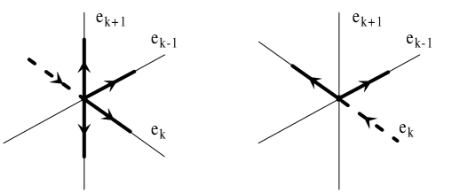
Figure 3:

In other words, the path can not move-up from an “affine subspace” (with the exception of the $\pm\mathbf{e}_{1}$ space) without first taking a step along the highest positive principle direction in the subspace. Similarly, the path can only move-down to an “affine subspace” by taking a positive first step along its highest principle direction. Otherwise, the path moves continuously.

Let $\text{\sf CGP}^{d}$ be: Given a triple $(G,0^{n},\mathbf{u}^{*})$ where $G$ is a canonical grid-PPAD graph over $\mathbb{Z}^{d}_{n}$ accessible by $\mathbb{B}_{G}$ and $\mathbf{u}^{*}$ is the starting vertex of $G$ with $u^{*}_{d}=1$, find the ending vertex of $G$. We use $\text{\sf RQ}_{\text{\sf CGP}}^{d}(n)$ to denote the randomized query complexity for solving this problem.

We now reduce $\text{\sf GP}^{d}$ to $\text{\sf CGP}^{d}$. Before stating and proving this result, we first give two geometric lemmas. They provide the local operations for canonicalization.

We start with some notation. A sequence $P=\mathbf{u}_{1}...\mathbf{u}_{m}$, for $m\geq 2$, is a canonical local path if $\mathbf{u}_{i}$’s are distinct elements from $\{-3,-2,...,+2,+3\}^{d}$ and $(\mathbf{u}_{i}-\mathbf{u}_{i-1},\mathbf{u}_{i+1}-\mathbf{u}_{i})\in\mathcal{S}^{d}$ for all $2\leq i\leq m-1$. Suppose $P=\mathbf{u}_{1}\mathbf{u}_{2}...\mathbf{u}_{m}$ and $Q=\mathbf{v}_{1}\mathbf{v}_{2}...\mathbf{v}_{k}$ are two paths with $\mathbf{u}_{m}=\mathbf{v}_{1}$. We use $P\diamond Q$ to denote their “concatenation”: $P\diamond Q=\mathbf{u}_{1}\mathbf{u}_{2}...\mathbf{u}_{m}\mathbf{v}_{2}...\mathbf{v}_{k}$.

Lemma 3.7 (Ending Gracefully).

For each $\mathbf{s}\in\mathbb{E}^{d}$ with $d\geq 2$, there is a canonical local path $P[d,\mathbf{s}]$ $=\mathbf{u}_{1}...\mathbf{u}_{m}$ satisfying $\mathbf{u}_{m}-\mathbf{u}_{m-1}=\mathbf{e}_{d}$, $\mathbf{u}_{1}=-3\mathbf{s}$, $\mathbf{u}_{2}=-2\mathbf{s}$, and $\forall\ i\in[2:m]$, $\|\mathbf{u}_{i}\|\leq 2$.

Proof.

We consider the three cases: $\mathbf{s}=\mathbf{e}_{l}$ for $1\leq l\leq d$, $\mathbf{s}=-\mathbf{e}_{1}$ and $\mathbf{s}=-\mathbf{e}_{l}$ for $2\leq l\leq d$.

In the first case, we set $P[d,\mathbf{s}]=\mathbf{u}_{1}\mathbf{u}_{2}...\mathbf{u}_{d-l+2}$ where $\mathbf{u}_{1}=-3\mathbf{e}_{l}$, $\mathbf{u}_{2}=-2\mathbf{e}_{l}$ and $\mathbf{u}_{i}=\mathbf{u}_{i-1}+\mathbf{e}_{l+i-2}$ for $3\leq i\leq d-l+2$. In the second case, we set $P[d,\mathbf{s}]=\mathbf{u}_{1}\mathbf{u}_{2}...\mathbf{u}_{d}\mathbf{u}_{d+1}$ where $\mathbf{u}_{1}=3\mathbf{e}_{1}$, $\mathbf{u}_{2}=2\mathbf{e}_{1}$ and $\mathbf{u}_{i}=\mathbf{u}_{i-1}+\mathbf{e}_{i-1}$ for $3\leq i\leq d+1$. In the third case, we set $P[d,\mathbf{s}]=\mathbf{u}_{1}\mathbf{u}_{2}...\mathbf{u}_{d-l+5}$ where $\mathbf{u}_{1}=3\mathbf{e}_{l}$, $\mathbf{u}_{2}=2\mathbf{e}_{l}$, $\mathbf{u}_{3}=\mathbf{e}_{l}$ and $\mathbf{u}_{i}=\mathbf{u}_{i-1}+\mathbf{e}_{l+i-5}$ for $4\leq i\leq d-l+5$.

One can easily check that $P[d,\mathbf{s}]$ satisfies the conditions of the lemma. ∎

Lemma 3.8 (Moving Gracefully).

For all $\mathbf{s}_{1},\mathbf{s}_{2}\in\mathbb{E}^{d}$ with $d\geq 2$ such that $\mathbf{s}_{1}+\mathbf{s}_{2}\not=0$, there exists a canonical local path $P[d,\mathbf{s}_{1},\mathbf{s}_{2}]=\mathbf{u}_{1}\mathbf{u}_{2}...\mathbf{u}_{m-1}\mathbf{u}_{m}$ that satisfies $\mathbf{u}_{1}=-3\mathbf{s}_{1}$, $\mathbf{u}_{2}=-2\mathbf{s}_{1}$, $\mathbf{u}_{m-1}=2\mathbf{s}_{2}$, $\mathbf{u}_{m}=3\mathbf{s}_{2}$, and $\forall\ i\in[2:m-1]$, $\|\mathbf{u}_{i}\|\leq 2$.

Proof.

We prove by induction on $d$ that there is a canonical local path $P[d,\mathbf{s}_{1},\mathbf{s}_{2}]$ such that

1. $P[d,\mathbf{s}_{1},\mathbf{s}_{2}]$ satisfies all the conditions in the statement of the lemma;

2. For all $\mathbf{s}_{1},\mathbf{s}_{2}\in\mathbb{E}^{d}$ such that $\mathbf{s}_{1}+\mathbf{s}_{2}\not=0$, $\mathbf{e}_{d},-\mathbf{e}_{d}\notin P[d,\mathbf{s}_{1},\mathbf{s}_{2}]$; and

3. If $\mathbf{s}_{1}=-\mathbf{e}_{d}$, then the first $3$ vertices of $P[d,-\mathbf{e}_{d},\mathbf{s}_{2}]$ are $3\mathbf{e}_{d}$, $2\mathbf{e}_{d}$ and $(\mathbf{e}_{d-1}+2\mathbf{e}_{d})$. If $\mathbf{s}_{2}=-\mathbf{e}_{d}$, then the last $3$ vertices of $P[d,\mathbf{s}_{1},-\mathbf{e}_{d}]$ are $(-\mathbf{e}_{d-1}-2\mathbf{e}_{d})$, $-2\mathbf{e}_{d}$ and $-3\mathbf{e}_{d}$.

The base case when $d=2$ is trivial. Inductively we assume, for $2\leq d^{\prime}<d$, path $P[d^{\prime},\mathbf{s}^{\prime}_{1},\mathbf{s}^{\prime}_{2}]$ exists for all $\mathbf{s}^{\prime}_{1},\mathbf{s}^{\prime}_{2}\in\mathbb{E}^{d^{\prime}}$ such that $\mathbf{s}^{\prime}_{1}+\mathbf{s}^{\prime}_{2}\not=0$. We let $P^{\prime}[d^{\prime},\mathbf{s}^{\prime}_{1},\mathbf{s}^{\prime}_{2}]$ denote the sub-path of $P[d^{\prime},\mathbf{s}^{\prime}_{1},\mathbf{s}^{\prime}_{2}]$ such that

$$P[d^{\prime},\mathbf{s}^{\prime}_{1},\mathbf{s}^{\prime}_{2}]=(-3\mathbf{s}^{\prime}_{1})\hskip 1.13791pt(-2\mathbf{s}^{\prime}_{1})\hskip 1.13791pt\diamond\hskip 1.13791ptP^{\prime}[d^{\prime},\mathbf{s}^{\prime}_{1},\mathbf{s}^{\prime}_{2}]\hskip 1.13791pt\diamond\hskip 1.13791pt(2\mathbf{s}^{\prime}_{2})\hskip 1.13791pt(3\mathbf{s}^{\prime}_{2}).$$

Note that $P^{\prime}[d^{\prime},\mathbf{s}^{\prime}_{1},\mathbf{s}^{\prime}_{2}]$ starts with $-2\mathbf{s}^{\prime}_{1}$ and ends with $+2\mathbf{s}^{\prime}_{2}$.

We will use $D$ to denote the map $D(\mathbf{r})=(r_{1},...,r_{d-1})$ from $\mathbb{Z}^{d}$ to $\mathbb{Z}^{d-1}$ and $U$ to denote the map $U(\mathbf{r})=(r_{1},...,r_{d-1},0)$ from $\mathbb{Z}^{d-1}$ to $\mathbb{Z}^{d}$. For a canonical local path $P=\mathbf{u}_{1}...\mathbf{u}_{m}$ in $\{-3,...,+3\}^{d-1}$, we use $U(P)$ to denote path $U(\mathbf{u}_{1})U(\mathbf{u}_{2})...U(\mathbf{u}_{m})$ in $\{-3,...,+3\}^{d}$.

For $\mathbf{s}_{1},\mathbf{s}_{2}\in\mathbb{E}^{d}$ with $\mathbf{s}_{1}+\mathbf{s}_{2}\not=0$, we use the following procedure to build $P[d,\mathbf{s}_{1},\mathbf{s}_{2}]$. Let

$$P^{+} = (-3\mathbf{e}_{d})\hskip 1.13791pt(-2\mathbf{e}_{d})\hskip 1.13791pt(\mathbf{e}_{d-1}-2\mathbf{e}_{d})\hskip 1.13791pt(\mathbf{e}_{d-1}-\mathbf{e}_{d})\hskip 1.13791pt(\mathbf{e}_{d-1})\hskip 1.13791pt(2\mathbf{e}_{d-1});$$

$$P^{-} = (3\mathbf{e}_{d})\hskip 1.13791pt(2\mathbf{e}_{d})\hskip 1.13791pt(\mathbf{e}_{d-1}+2\mathbf{e}_{d})\hskip 1.13791pt(\mathbf{e}_{d-1}+\mathbf{e}_{d})\hskip 1.13791pt(\mathbf{e}_{d-1})\hskip 1.13791pt(2\mathbf{e}_{d-1});$$

$$Q^{+} = (-2\mathbf{e}_{d-1})\hskip 1.13791pt(-\mathbf{e}_{d-1})\hskip 1.13791pt(-\mathbf{e}_{d-1}+\mathbf{e}_{d})\hskip 1.13791pt(-\mathbf{e}_{d-1}+2\mathbf{e}_{d})\hskip 1.13791pt(2\mathbf{e}_{d})\hskip 1.13791pt(3\mathbf{e}_{d});$$

$$Q^{-} = (-2\mathbf{e}_{d-1})\hskip 1.13791pt(-\mathbf{e}_{d-1})\hskip 1.13791pt(-\mathbf{e}_{d-1}-\mathbf{e}_{d})\hskip 1.13791pt(-\mathbf{e}_{d-1}-2\mathbf{e}_{d})\hskip 1.13791pt(-2\mathbf{e}_{d})\hskip 1.13791pt(-3\mathbf{e}_{d}).$$

• If $\mathbf{s}_{1}\notin\{\pm\mathbf{e}_{d}\}$, then set $P=(-3\mathbf{s}_{1})(-2\mathbf{s}_{1})$ and $\mathbf{s}_{1}^{\prime}=D(\mathbf{s}_{1})$;

  Set $P=P^{+}$ and $\mathbf{s}_{1}^{\prime}=-\mathbf{e}_{d-1}$ if $\mathbf{s}_{1}=\mathbf{e}_{d}$ and $P=P^{-}$ and $\mathbf{s}_{1}^{\prime}=-\mathbf{e}_{d-1}$ if $\mathbf{s}_{1}=-\mathbf{e}_{d}$;

• If $\mathbf{s}_{2}\notin\{\pm\mathbf{e}_{d}\}$, then set $Q=(2\mathbf{s}_{2})(3\mathbf{s}_{2})$ and $\mathbf{s}_{2}^{\prime}=D(\mathbf{s}_{2})$;

  Set $Q=Q^{+}$ and $\mathbf{s}_{2}^{\prime}=-\mathbf{e}_{d-1}$ if $\mathbf{s}_{2}=\mathbf{e}_{d}$ and $Q=Q^{-}$ and $\mathbf{s}_{2}^{\prime}=-\mathbf{e}_{d-1}$ if $\mathbf{s}_{2}=-\mathbf{e}_{d}$;

• Set $P[d,\mathbf{s}_{1},\mathbf{s}_{2}]=P\hskip 1.13791pt\diamond\hskip 1.13791ptU(P^{\prime}[d-1,\mathbf{s}_{1}^{\prime},\mathbf{s}_{2}^{\prime}])\hskip 1.13791pt\diamond\hskip 1.13791ptQ$:

One can check that $P[d,\mathbf{s}_{1},\mathbf{s}_{2}]$ satisfies all three conditions of the inductive statement. ∎

Theorem 3.9 (Canonicalization).

For all $d\geq 2$, $\text{\sf RQ}_{\text{\sf GP}}^{d}(n)\leq\text{\sf RQ}_{\text{\sf CGP}}^{d}(6n+1)$.

Proof.

Let $\Gamma(\mathbf{u})=6\mathbf{u}-\mathbf{2}$ be a map from $\mathbb{Z}^{d}$ to $\mathbb{Z}^{d}$. Given any grid-PPAD graph $G^{*}$ over $\mathbb{Z}^{d}_{n}$, we now use the canonical local paths provided in Lemmas 3.7 and 3.8 to build a canonical grid-PPAD graph $G=(\mathbb{Z}_{6n+1}^{d},E)$. In the procedure below, initially $E=\emptyset$:

1. [ canonicalizing the starting vertex ]: Let $\mathbf{u}^{*}$ be the starting vertex of $G^{*}$. Suppose $\mathbb{B}_{G^{*}}(\mathbf{u}^{*})=(\text{``no''},\mathbf{s})$. As $u^{*}_{d}=1$, we have $\mathbf{s}\not=-\mathbf{e}_{d}$. For every edge $(\mathbf{v}_{1},\mathbf{v}_{2})$ appears in path $P[d,\mathbf{e}_{d},\mathbf{s}]$, add $(\Gamma(\mathbf{u}^{*})+\mathbf{v}_{1},\Gamma(\mathbf{u}^{*})+\mathbf{v}_{2})$ to $E$;

2. [ canonicalizing the ending vertex ]: Let $\mathbf{w}^{*}$ be the ending vertex of $G^{*}$. Suppose $\mathbb{B}_{G^{*}}(\mathbf{w}^{*})=(\mathbf{s},\text{``no''})$. For every $(\mathbf{v}_{1},\mathbf{v}_{2})$ in $P[d,\mathbf{s}]$, add $(\Gamma(\mathbf{w}^{*})+\mathbf{v}_{1},\Gamma(\mathbf{w}^{*})+\mathbf{v}_{2})$ to $E$;

3. [ canonicalizing other vertices ]: For all $\mathbf{u}\in\mathbb{Z}^{d}_{n}-\{\mathbf{u}^{*},\mathbf{w}^{*}\}$, if $\mathbb{B}_{G^{*}}(\mathbf{u})=(\mathbf{s}_{1},\mathbf{s}_{2})$ and $\mathbf{s}_{1},\mathbf{s}_{2}\not=\text{``no''}$, then add $(\Gamma(\mathbf{u})+\mathbf{v}_{1},\Gamma(\mathbf{u})+\mathbf{v}_{2})$ to $E$ for every edge $(\mathbf{v}_{1},\mathbf{v}_{2})$ in $P[d,\mathbf{s}_{1},\mathbf{s}_{2}]$.

By Lemmas 3.7, 3.8 and the procedure above, $G=(\mathbb{Z}_{6n+1}^{d},E)$ is a canonical grid-PPAD graph that satisfies the following two properties, from which Theorem 3.9 follows.

  (C.1)

The starting vertex of $G$ is $\Gamma(\mathbf{u}^{*})-3\mathbf{e}_{d}$, and the ending vertex $\mathbf{w}$ of $G$ satisfies $\|\mathbf{w}-\Gamma(\mathbf{w}^{*})\|\leq 2$.

  (C.2)

For every vertex $\mathbf{v}\in G$, to determine $\mathbb{B}_{G}(\mathbf{v})$, one only need to know $\mathbb{B}_{G^{*}}(\mathbf{u})$ where $\mathbf{u}$ is the lexicographically smallest vertex in $\mathbb{Z}_{n}^{d}$ such that $\|\mathbf{v}-\Gamma(\mathbf{u})\|\leq 3$.

∎

3.3 From $\text{\sf CGP}^{d}$ to $\text{\sf ZP}^{d}$: Complete the Proof of Theorem 3.2

Now we reduce $\text{\sf CGP}^{d}$ to $\text{\sf ZP}^{d}$. The main task of this section is to, given a canonical grid-PPAD graph $G=(\mathbb{Z}^{d}_{n},E)$ and its starting vertex $\mathbf{u}^{*}$, construct a discrete Brouwer function $f_{G}:\mathbb{Z}^{d}_{4n+2}\rightarrow\{\hskip 1.13791pt\mathbf{0}\hskip 1.13791pt\}\cup\mathbb{E}^{d}$ that satisfies the following two properties:

  (D.1)

$f_{G}$ has exactly one zero point $\mathbf{r}^{*}$, and $\Psi^{-1}(\mathbf{r}^{*})$ is the ending vertex of $G$, and

  (D.2)

For each $\mathbf{r}\in\mathbb{Z}^{d}_{4n+2}$, at most one query to $\mathbb{B}_{G}$ is needed to evaluate $f_{G}$,

where $\Psi(\mathbf{u})=4\mathbf{u}$ is a map from $\mathbb{Z}^{d}_{n}$ to $\mathbb{Z}^{d}_{4n+2}$. Immediately from these properties, we have

Theorem 3.10 (From $\text{\sf CGP}^{d}$ to $\text{\sf ZP}^{d}$).

For all $d\geq 2$, $\text{\sf RQ}_{\text{\sf CGP}}^{d}(n)\leq\text{\sf RQ}_{\text{\sf ZP}}^{d}(4n+2).$

Local Geometry of Canonical Grid PPAD Graphs

To construct a Brouwer function from $G=(\mathbb{Z}^{d}_{n},E)$, we define a set $\mathcal{I}_{G}\subset\mathbb{Z}^{d}_{4n+2}$, which looks like a collection of pipes, to embed and insulate the component of $G$. $\mathcal{I}_{G}$ has two parts, a kernel $\mathcal{K}_{G}$ and a boundary $\mathcal{B}_{G}$. We will first construct a direction-preserving function $f^{G}$ on $\mathcal{B}_{G}$. We then extend the function onto $\mathbb{Z}^{d}_{4n+2}$ to define $f_{G}$. In our presentation, we will only use $\mathbf{u},\mathbf{v},\mathbf{w}$ to denote vertices in $\mathbb{Z}^{d}_{n}$ and use $\mathbf{p},\mathbf{q},\mathbf{r}$ to denote points in $\mathbb{Z}^{d}_{4n+2}$. Let $\mathbf{u}$ and $\mathbf{v}$ be two vertices in $\mathbb{Z}^{d}_{n}$ with $\mathbf{u}-\mathbf{v}\in\mathbb{E}^{d}$. We abuse $\Psi(\mathbf{u}\mathbf{v})$ to denote the set of five integer points on line segment $\Psi(\mathbf{u})\Psi(\mathbf{v})$. Let $\mathbf{u}^{*}$ and $\mathbf{w}^{*}$ be the starting and ending vertices of $G$. We define

$$\mathcal{K}_{G}=\left(\hskip 1.42271pt\bigcup_{(\mathbf{v}_{1},\mathbf{v}_{2})\in E}\Psi(\mathbf{v}_{1}\mathbf{v}_{2})\hskip 1.42271pt\right)\cup\Big{\{}\hskip 2.27626pt\Psi(\mathbf{u}^{*})-\mathbf{e}_{d},\Psi(\mathbf{w}^{*})+\mathbf{e}_{d}\hskip 2.27626pt\Big{\}},$$

$$\mathcal{B}_{G}=\Big{\{}\hskip 2.27626pt\mathbf{r}\notin\mathcal{K}_{G}\hskip 2.84544pt\Big{|}\hskip 2.84544pt\exists\ \mathbf{r}^{\prime}\in\bigcup_{(\mathbf{v}_{1},\mathbf{v}_{2})\in E}\Psi(\mathbf{v}_{1}\mathbf{v}_{2}),\|\mathbf{r}-\mathbf{r}^{\prime}\|=1\hskip 2.27626pt\Big{\}},$$

and $\mathcal{I}_{G}=\mathcal{K}_{G}\cup\mathcal{B}_{G}$. For $\mathbf{u}\in\mathbb{Z}^{d}_{n}$, we use $\mathcal{C}_{\mathbf{u}}$ to denote $\{\hskip 1.42271pt\mathbf{r}\in\mathbb{Z}^{d}_{4n+2},\|\mathbf{r}-\Psi(\mathbf{u})\|\leq 2\hskip 1.42271pt\}$. As the local structure of $\mathcal{B}_{G}\cap\mathcal{C}_{\mathbf{u}}$ depends only on $\mathbb{B}_{G}(\mathbf{u})$, we introduce the following definitions.

Definition 3.11 (Local Kernel and Boundary).

For each pair $\pi=(\mathbf{s}_{1},\mathbf{s}_{2})\in\mathcal{S}^{d}$ with $d\geq 2$, let $\mathcal{K}_{d,\pi}$ and $\mathcal{B}_{d,\pi}$ be two subsets of $\mathbb{Z}^{d}_{[-2,2]}=\{-2,-1,0,1,2\}^{d}$, such that

1. if $\mathbf{s}_{1}=\mathbf{s}_{2}=\text{``no''}$, then $\mathcal{K}_{d,\pi}=\mathcal{B}_{d,\pi}=\emptyset$;

2. if $\mathbf{s}_{1}=\text{``no''}$ and $\mathbf{s}_{2}\not=\text{``no''}$ ($\mathbf{s}_{2}=\mathbf{e}_{d}$), then $\mathcal{K}_{d,\pi}=\{-\mathbf{e}_{d},\mathbf{0},\mathbf{e}_{d},2\mathbf{e}_{d}\}$ and

   $$\mathcal{B}_{d,\pi}=\big{\{}\hskip 2.27626pt\mathbf{r}\in\mathbb{Z}^{d}_{[-2,2]}-\mathcal{K}_{d,\pi}\hskip 2.84544pt\big{|}\hskip 2.84544pt\exists\ \mathbf{r}^{\prime}\in\{\mathbf{0},\mathbf{e}_{d},2\mathbf{e}_{d}\hskip 1.70709pt\},\|\mathbf{r}-\mathbf{r}^{\prime}\|=1\hskip 1.70709pt\big{\}};\vspace{-0.2cm}$$

3. if $\mathbf{s}_{1}\not=\text{``no''}$ and $\mathbf{s}_{2}=\text{``no''}$ ($\mathbf{s}_{1}=\mathbf{e}_{d}$), then $\mathcal{K}_{d,\pi}=\{-2\mathbf{e}_{d},-\mathbf{e}_{d},\mathbf{0},\mathbf{e}_{d}\}$ and

   $$\mathcal{B}_{d,\pi}=\big{\{}\hskip 2.27626pt\mathbf{r}\in\mathbb{Z}^{d}_{[-2,2]}-\mathcal{K}_{d,\pi}\hskip 2.84544pt\big{|}\hskip 2.84544pt\exists\ \mathbf{r}^{\prime}\in\{-2\mathbf{e}_{d},-\mathbf{e}_{d},\mathbf{0}\},\|\mathbf{r}-\mathbf{r}^{\prime}\|=1\hskip 1.70709pt\big{\}};\vspace{-0.2cm}$$

4. otherwise, $\mathcal{K}_{d,\pi}=\{-2\mathbf{s}_{1},-\mathbf{s}_{1},0,\mathbf{s}_{2},2\mathbf{s}_{2}\}$ and

   $$\mathcal{B}_{d,\pi}=\big{\{}\hskip 2.27626pt\mathbf{r}\in\mathbb{Z}^{d}_{[-2,2]}-\mathcal{K}_{d,\pi}\hskip 2.84544pt\big{|}\hskip 2.84544pt\exists\ \mathbf{r}^{\prime}\in\mathcal{K}_{d,\pi},\|\mathbf{r}-\mathbf{r}^{\prime}\|=1\hskip 1.70709pt\big{\}}.\vspace{-0.2cm}$$

For $\mathbf{r}\in\mathbb{Z}^{d}$ and set $S\subseteq\mathbb{Z}^{d}$, let $\mathbf{r}+S=\{\hskip 1.13791pt\mathbf{r}+\mathbf{r}^{\prime},\mathbf{r}^{\prime}\in S\hskip 1.13791pt\}$. We will use the fact that for all $\mathbf{u}\in\mathbb{Z}^{d}_{n}$, if $\pi=\mathbb{B}_{G}(\mathbf{u})$, then $\mathcal{K}_{G}\cap\mathcal{C}_{\mathbf{u}}=\Psi(\mathbf{u})+\mathcal{K}_{d,\pi}$ and $\mathcal{B}_{G}\cap\mathcal{C}_{\mathbf{u}}=\Psi(\mathbf{u})+\mathcal{B}_{d,\pi}$.

The Construction of Brouwer Function

First, we define two direction-preserving functions $f_{d,+},f_{d,-}$ from $\mathcal{B}_{d}$ to $\mathbb{E}^{d}$ for $d\geq 2$, where $\mathcal{B}_{d}=\{\hskip 1.13791pt-1,0,1\hskip 1.13791pt\}^{d}-\mathbf{0}$: For every $\mathbf{r}\in\mathcal{B}_{d}$, letting $k$ be the smallest integer such that $r_{k}\not=0$, $f_{d,+}(\mathbf{r})=f_{d,-}(\mathbf{r})=-r_{k}\mathbf{e}_{k}$ if $1\leq k\leq d-1$ and $f_{d,+}(\mathbf{r})=-r_{d}\mathbf{e}_{d}$, $f_{d,-}(\mathbf{r})=r_{d}\mathbf{e}_{d}$, otherwise. Using these two functions, we inductively build a ( direction-preserving ) function $f_{d,\pi}$ on $\mathcal{B}_{d,\pi}$ for each $\pi=(\mathbf{s}_{1},\mathbf{s}_{2})\in\mathcal{S}^{d}$. See Figure 4 for the complete construction for $d=2$. Informally, if $\mathbf{r}\in\mathcal{B}_{2,\pi}$ is on the left side of the “local” path, then $f_{2,\pi}(\mathbf{r})=-\mathbf{e}_{1}$, otherwise it equals $\mathbf{e}_{1}$.

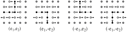
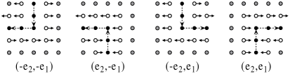
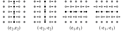
Figure 4: $f_{2,\pi}$, $f_{2,+}$ and $f_{2,-}$

For $d\geq 3$, the construction is more complex but relatively procedural. Below, we use $D$ to denote the map $D(\mathbf{r})=(r_{1},r_{2},...,r_{d-1})$ from $\mathbb{Z}^{d}$ to $\mathbb{Z}^{d-1}$ and $U_{k}$ to denote the map $U_{k}(\mathbf{r})=(r_{1},r_{2},...,r_{d-1},k)$ from $\mathbb{Z}^{d-1}$ to $\mathbb{Z}^{d}$; we also extends it to sets, that is, $U_{k}(S)=\{\hskip 1.13791ptU_{k}(\mathbf{r}),\mathbf{r}\in S\hskip 1.13791pt\}$ for $S\subset\mathbb{Z}^{d-1}$. Let $S[k]=\{\hskip 1.13791pt\mathbf{r}\in S,r_{d}=k\hskip 1.13791pt\}$ for $S\subset\mathbb{Z}^{d}$.

1. Moving within (d-1)-dimensional space:

   When $\pi=(\mathbf{s}_{1},\mathbf{s}_{2})$ satisfies $\pi^{\prime}=(D(\mathbf{s}_{1}),D(\mathbf{s}_{2}))\in\mathcal{S}^{d-1}$, $\mathcal{B}_{d,\pi}$ can be decomposed into

   $$\left(U_{-1}(\mathcal{B}_{d-1,\pi^{\prime}})\hskip 1.13791pt\cup\hskip 1.13791ptU_{-1}(\mathcal{K}_{d-1,\pi^{\prime}})\right)\hskip 1.70709pt\cup\hskip 1.70709ptU_{0}(\mathcal{B}_{d-1,\pi^{\prime}})\hskip 1.70709pt\cup\hskip 1.70709pt\left(U_{1}(\mathcal{B}_{d-1,\pi^{\prime}})\hskip 1.13791pt\cup\hskip 1.13791ptU_{1}(\mathcal{K}_{d-1,\pi^{\prime}})\right).\vspace{-0.05cm}$$

   We set $f_{d,\pi}(\mathbf{r})=U_{0}(f_{d-1,\pi^{\prime}}(D(\mathbf{r})))$ for $\mathbf{r}\in U_{-1}(\mathcal{B}_{d-1,\pi^{\prime}})\cup U_{0}(\mathcal{B}_{d-1,\pi^{\prime}})\cup U_{1}(\mathcal{B}_{d-1,\pi^{\prime}})$.

   We set $f_{d,\pi}(\mathbf{r})=-\mathbf{e}_{d-1}$ for $\mathbf{r}\in U_{-1}(\mathcal{K}_{d-1,\pi^{\prime}})$ and $f_{d,\pi}(\mathbf{r})=\mathbf{e}_{d-1}$ for $\mathbf{r}\in U_{1}(\mathcal{K}_{d-1,\pi^{\prime}})$.

2. Moving along $\pm\mathbf{e}_{d}$: In this case, we will use the fact $D(\mathbf{r})\in\mathcal{B}_{d-1}$, for all $\mathbf{r}\in\mathcal{B}_{d,\pi}$.

   When $\pi=(\mathbf{e}_{d},\mathbf{e}_{d})$, $(\text{``no''},\mathbf{e}_{d})$ or $(\mathbf{e}_{d},\text{``no''})$, $f_{d,\pi}(\mathbf{r})=U_{0}(f_{d-1,+}(D(\mathbf{r})))$ for all $\mathbf{r}\in\mathcal{B}_{d,\pi}$.

   When $\pi=(-\mathbf{e}_{d},-\mathbf{e}_{d})$, we set $f_{d,\pi}(\mathbf{r})=U_{0}(f_{d-1,-}(D(\mathbf{r})))$ for all $\mathbf{r}\in\mathcal{B}_{d,\pi}$.

3. Moving between $\mathbf{e}_{d-1}$ and $\pm\mathbf{e}_{d}$:

   1. When $\pi=(\mathbf{s}_{1},\mathbf{s}_{2})=(\mathbf{e}_{d-1},\mathbf{e}_{d})$, let $\pi^{\prime}=(D(\mathbf{s}_{1}),\text{``no''})\in\mathcal{S}^{d-1}$. We have

      $$\mathcal{B}_{d,\pi}[2]=U_{2}(\mathcal{B}_{d-1}),\ \mathcal{B}_{d,\pi}[1]=U_{1}(\mathcal{B}_{d-1,\pi^{\prime}}\cup\mathcal{K}_{d-1,\pi^{\prime}})-\{\mathbf{e}_{d}\},\mathcal{B}_{d,\pi}[-2]=\emptyset,$$

      $$\mathcal{B}_{d,\pi}[0]=U_{0}(\mathcal{B}_{d-1,\pi^{\prime}})\cup\{\mathbf{e}_{d-1}\},\ \mathcal{B}_{d,\pi}[-1]=U_{-1}(\mathcal{B}_{d-1,\pi^{\prime}}\cup\mathcal{K}_{d-1,\pi^{\prime}}).$$

      We set $f_{d,\pi}(\mathbf{r})=U_{0}(f_{d-1,+}(D(\mathbf{r})))$ for $\mathbf{r}\in\mathcal{B}_{d,\pi}[2]$;

      $f_{d,\pi}(\mathbf{r})=U_{0}(f_{d-1,\pi^{\prime}}(D(\mathbf{r})))$ for $\mathbf{r}\in U_{1}(\mathcal{B}_{d-1,\pi^{\prime}})\cup U_{0}(\mathcal{B}_{d-1,\pi^{\prime}})\cup U_{-1}(\mathcal{B}_{d-1,\pi^{\prime}})$;

      $f_{d,\pi}(\mathbf{e}_{d-1}+\mathbf{e}_{d})=f_{d,\pi}(\mathbf{e}_{d-1})=-\mathbf{e}_{d-1}$; $f_{d,\pi}(\mathbf{r})=-\mathbf{e}_{d-1}$ for $\mathbf{r}\in U_{-1}(\mathcal{K}_{d-1,\pi^{\prime}})$;

      $f_{d,\pi}(\mathbf{r})=\mathbf{e}_{d-1}$ for $\mathbf{r}\in U_{1}(\mathcal{K}_{d-1,\pi^{\prime}})-\{\mathbf{e}_{d},\mathbf{e}_{d-1}+\mathbf{e}_{d}\}$.

   2. When $\pi=(\mathbf{s}_{1},\mathbf{s}_{2})=(-\mathbf{e}_{d},\mathbf{e}_{d-1})$, let $\pi^{\prime}=(\text{``no''},D(\mathbf{s}_{2}))\in\mathcal{S}^{d-1}$. We have

      $$\mathcal{B}_{d,\pi}[-2]=\emptyset,\ \mathcal{B}_{d,\pi}[2]=U_{2}(\mathcal{B}_{d-1}),\ \mathcal{B}_{d,\pi}[1]=U_{1}(\mathcal{B}_{d-1,\pi^{\prime}}\cup\mathcal{K}_{d-1,\pi^{\prime}})-\{\mathbf{e}_{d}\},$$

      $$\mathcal{B}_{d,\pi}[0]=U_{0}(\mathcal{B}_{d-1,\pi^{\prime}})\cup\{-\mathbf{e}_{d-1}\},\ \mathcal{B}_{d,\pi}[-1]=U_{-1}(\mathcal{B}_{d-1,\pi^{\prime}}\cup\mathcal{K}_{d-1,\pi^{\prime}}).$$

      We set $f_{d,\pi}(\mathbf{r})=U_{0}(f_{d-1,-}(D(\mathbf{r})))$ for $\mathbf{r}\in\mathcal{B}_{d,\pi}[2]$;

      $f_{d,\pi}(\mathbf{r})=U_{0}(f_{d-1,\pi^{\prime}}(D(\mathbf{r})))$ for $\mathbf{r}\in U_{1}(\mathcal{B}_{d-1,\pi^{\prime}})\cup U_{0}(\mathcal{B}_{d-1,\pi^{\prime}})\cup U_{-1}(\mathcal{B}_{d-1,\pi^{\prime}})$;

      $f_{d,\pi}(\mathbf{r})=-\mathbf{e}_{d-1}$ for $\mathbf{r}\in U_{-1}(\mathcal{K}_{d-1,\pi^{\prime}})$; $f_{d,\pi}(-\mathbf{e}_{d-1}+\mathbf{e}_{d})=f_{d,\pi}(-\mathbf{e}_{d-1})=-\mathbf{e}_{d-1}$;

      $f_{d,\pi}(\mathbf{r})=\mathbf{e}_{d-1}$ for $\mathbf{r}\in U_{1}(\mathcal{K}_{d-1,\pi^{\prime}})-\{-\mathbf{e}_{d-1}+\mathbf{e}_{d},\mathbf{e}_{d}\}$.

      

      

      

      

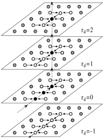
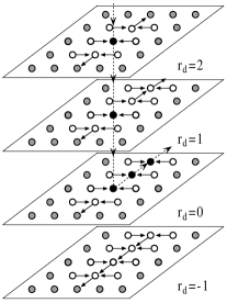
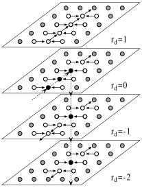
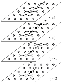
      Figure 5: $f_{3,\pi}$ where $\pi=(\mathbf{e}_{d-1},\mathbf{e}_{d}),(-\mathbf{e}_{d},\mathbf{e}_{d-1}),(\mathbf{e}_{d-1},-\mathbf{e}_{d})$ and $(\mathbf{e}_{d},\mathbf{e}_{d-1})$

   3. When $\pi=(\mathbf{s}_{1},\mathbf{s}_{2})=(\mathbf{e}_{d-1},-\mathbf{e}_{d})$, let $\pi^{\prime}=(D(\mathbf{s}_{1}),\text{``no''})\in\mathcal{S}^{d-1}$. We have

      $$\mathcal{B}_{d,\pi}[2]=\emptyset,\ \mathcal{B}_{d,\pi}[1]=U_{1}(\mathcal{B}_{d-1,\pi^{\prime}}\cup\mathcal{K}_{d-1,\pi^{\prime}}),\ \mathcal{B}_{d,\pi}[0]=U_{0}(\mathcal{B}_{d-1,\pi^{\prime}})\cup\{\mathbf{e}_{d-1}\},$$

      $$\mathcal{B}_{d,\pi}[-1]=U_{-1}(\mathcal{B}_{d-1,\pi^{\prime}}\cup\mathcal{K}_{d-1,\pi^{\prime}})-\{-\mathbf{e}_{d}\},\ \mathcal{B}_{d,\pi}[-2]=U_{-2}(\mathcal{B}_{d-1}).$$

      We set $f_{d,\pi}(\mathbf{r})=U_{0}(f_{d-1,-}(D(\mathbf{r})))$ for $\mathbf{r}\in\mathcal{B}_{d,\pi}[-2]$;

      $f_{d,\pi}(\mathbf{r})=U_{0}(f_{d-1,\pi^{\prime}}(D(\mathbf{r})))$ for $\mathbf{r}\in U_{1}(\mathcal{B}_{d-1,\pi^{\prime}})\cup U_{0}(\mathcal{B}_{d-1,\pi^{\prime}})\cup U_{-1}(\mathcal{B}_{d-1,\pi^{\prime}})$;

      $f_{d,\pi}(\mathbf{r})=\mathbf{e}_{d-1}$ for $\mathbf{r}\in U_{1}(\mathcal{K}_{d-1,\pi^{\prime}})$; $f_{d,\pi}(\mathbf{e}_{d-1})=f_{d,\pi}(\mathbf{e}_{d-1}-\mathbf{e}_{d})=\mathbf{e}_{d-1}$;

      $f_{d,\pi}(\mathbf{r})=-\mathbf{e}_{d-1}$ for $\mathbf{r}\in U_{-1}(\mathcal{K}_{d-1,\pi^{\prime}})-\{-\mathbf{e}_{d},\mathbf{e}_{d-1}-\mathbf{e}_{d}\}$.

   4. When $\pi=(\mathbf{s}_{1},\mathbf{s}_{2})=(\mathbf{e}_{d},\mathbf{e}_{d-1})$, let $\pi^{\prime}=(\text{``no''},D(\mathbf{s}_{2}))\in\mathcal{S}^{d-1}$. We have

      $$\mathcal{B}_{d,\pi}[2]=\emptyset,\ \mathcal{B}_{d,\pi}[1]=U_{1}(\mathcal{B}_{d-1,\pi^{\prime}}\cup\mathcal{K}_{d-1,\pi^{\prime}}),\ \mathcal{B}_{d,\pi}[0]=U_{0}(\mathcal{B}_{d-1,\pi^{\prime}})\cup\{-\mathbf{e}_{d-1}\},$$

      $$\mathcal{B}_{d,\pi}[-1]=U_{-1}(\mathcal{B}_{d-1,\pi^{\prime}}\cup\mathcal{K}_{d-1,\pi^{\prime}})-\{-\mathbf{e}_{d}\},\ \mathcal{B}_{d,\pi}[-2]=U_{-2}(\mathcal{B}_{d-1}).$$

      We set $f_{d,\pi}(\mathbf{r})=U_{0}(f_{d-1,+}(D(\mathbf{r})))$ for $\mathbf{r}\in\mathcal{B}_{d,\pi}[-2]$;

      $f_{d,\pi}(\mathbf{r})=U_{0}(f_{d-1,\pi^{\prime}}(D(\mathbf{r})))$ for $\mathbf{r}\in U_{1}(\mathcal{B}_{d-1,\pi^{\prime}})\cup U_{0}(\mathcal{B}_{d-1,\pi^{\prime}})\cup U_{-1}(\mathcal{B}_{d-1,\pi^{\prime}})$;

      $f_{d,\pi}(\mathbf{r})=\mathbf{e}_{d-1}$ for $\mathbf{r}\in U_{1}(\mathcal{K}_{d-1,\pi^{\prime}})$; $f_{d,\pi}(-\mathbf{e}_{d-1})=f_{d,\pi}(-\mathbf{e}_{d-1}-\mathbf{e}_{d})=\mathbf{e}_{d-1}$;

      $f_{d,\pi}(\mathbf{r})=-\mathbf{e}_{d-1}$ for $\mathbf{r}\in U_{-1}(\mathcal{K}_{d-1,\pi^{\prime}}))-\{-\mathbf{e}_{d},-\mathbf{e}_{d-1}-\mathbf{e}_{d}\}$.

Lemma 3.12 (Locally Directional Preserving).

For every $\pi\in\mathcal{S}^{d}$, $f_{d,\pi}$ is direction-preserving on $\mathcal{B}_{d,\pi}$.

Proof.

We prove the lemma by induction on $d$. The base case when $d=2$ is trivial. We now consider the case when $d>2$ and assume inductively that the statement is true for $d-1$.

First, $\pi=(\mathbf{e}_{d},\mathbf{e}_{d})$, $(\text{``no''},\mathbf{e}_{d})$, $(\mathbf{e}_{d},\text{``no''})$ or $(-\mathbf{e}_{d},-\mathbf{e}_{d})$. The statement follows from the fact that $f_{d-1,+}$ and $f_{d-1,-}$ are direction-preserving on $\mathcal{B}_{d-1}$. Second, $\pi=(\mathbf{s}_{1},\mathbf{s}_{2})$ satisfies $\pi^{\prime}=(D(\mathbf{s}_{1}),D(\mathbf{s}_{2}))\in\mathcal{S}^{d-1}$. By the inductive hypothesis, $f_{d-1,\pi^{\prime}}$ is direction-preserving, from which the statement follows. Third, $\pi=(\mathbf{e}_{d-1},\mathbf{e}_{d})$, $(\mathbf{e}_{d-1},-\mathbf{e}_{d})$, $(-\mathbf{e}_{d},\mathbf{e}_{d-1})$ or $(\mathbf{e}_{d},\mathbf{e}_{d-1})$. One can prove the following statement by induction on $d$.

For $\pi_{1}=(\text{``no''},\mathbf{e}_{d})$ and $\pi_{2}=(\mathbf{e}_{d},\text{``no''})$, $\mathcal{B}_{d,\pi_{1}}\cap\mathcal{B}_{d}=\mathcal{B}_{d,\pi_{2}}\cap\mathcal{B}_{d}=\mathcal{B}_{d}-\{-\mathbf{e}_{d},\mathbf{e}_{d}\}$. Moreover for each $\mathbf{r}\in\mathcal{B}_{d}-\{-\mathbf{e}_{d},\mathbf{e}_{d}\}$, $f_{d,\pi_{1}}(\mathbf{r})=f_{d,\pi_{2}}(\mathbf{r})=f_{d,+}(\mathbf{r})=f_{d,-}(\mathbf{r})$.

To show $f_{d,\pi}$ is direction-preserving on $\mathcal{B}_{d,\pi}$, it suffices to check $\|\mathbf{r}_{1}-\mathbf{r}_{2}\|>1$, for all pairs $\mathbf{r}_{1},\mathbf{r}_{2}\in\mathcal{B}_{d,\pi}$ such that$f_{d,\pi}(\mathbf{r}_{1})=\mathbf{e}_{d-1}$ and $f_{d,\pi}(\mathbf{r}_{2})=-\mathbf{e}_{d-1}$. ∎

With these local functions $f_{d,\pi}$, we can build a global function $f^{G}$ from $\mathcal{B}_{G}$ to $\{\pm\mathbf{e}_{1},...,$ $\pm\mathbf{e}_{d-1}\}$ as following: for every $\mathbf{r}\in\mathcal{B}_{G}$, we set $f^{G}(\mathbf{r})=f_{d,\pi}(\mathbf{r}-\Psi(\mathbf{u}))$, where $\mathbf{u}$ is the lexicographically smallest vertex in $\mathbb{Z}^{d}_{n}$ such that $\mathbf{r}\in\mathcal{C}_{\mathbf{u}}$ and $\pi=\mathbb{B}_{G}(\mathbf{u})$,

 

$f_{G}(\mathbf{r})$, where $\mathbf{r}\in\mathbb{Z}^{d}_{4n+2}$

 

1 :	let $\mathbf{u}^{*}$ and $\mathbf{w}^{*}$ be the starting and ending vertices of $G$, $\mathbf{p}^{*}=\Psi(\mathbf{u}^{*})$ and $\mathbf{q}^{*}=\Psi(\mathbf{w}^{*})$
2 :	if $r_{d}=1$ or $2$, and $D(\mathbf{r})=D(\mathbf{p}^{*})$ then $f_{G}(\mathbf{r})=\mathbf{e}_{d}$
3 :	else if $r_{d}=1$ or $2$, and $\|D(\mathbf{r})-D(\mathbf{p}^{*})\|=1$ then
4 :	let $k$ denote the smallest integer such that $r_{k}\not=r^{*}_{k}$, $f_{G}(\mathbf{r})=(p^{*}_{k}-r_{k})\mathbf{e}_{k}$
5 :	else if $\mathbf{r}=\mathbf{q}^{*}$ then $f_{G}(\mathbf{r})=0$
6 :	else if $\mathbf{r}=\mathbf{q}^{*}+\mathbf{e}_{d}$ then $f_{G}(\mathbf{r})=-\mathbf{e}_{d}$
7 :	else if $\mathbf{r}\in\mathcal{K}_{G}$ then $f_{G}(\mathbf{r})=\mathbf{e}_{d}$
8 :	else if $\mathbf{r}\in\mathcal{B}_{G}$ then $f_{G}(\mathbf{r})=f^{G}(\mathbf{r})$
9 :	else if $r_{d}=1$ (and $\|D(\mathbf{r})-D(\mathbf{p}^{*})\|\geq 2$) then
10 :	let $k$ denote the smallest integer such that $r_{k}\not=r^{*}_{k}$, $f_{G}(\mathbf{r})=\text{sign}(p^{*}_{k}-r_{k})\mathbf{e}_{k}$
11 :	else $f_{G}(\mathbf{r})=-\mathbf{e}_{d}$

 

Figure 6: Construction of Function $f_{G}$ from $f^{G}$

Lemma 3.13.

For every canonical grid PPAD graph $G$ over $\mathbb{Z}^{d}_{n}$, $f^{G}$ is direction-preserving on set $\mathcal{B}_{G}$.

Proof.

By Lemma 3.12, it suffices to prove the following: For $\mathbf{r}\in\mathcal{B}_{G}$, if $\mathbf{r}\in\mathcal{C}_{\mathbf{u}}\cap\mathcal{C}_{\mathbf{v}}$ where $\mathbf{u},$ $\mathbf{v}\in\mathbb{Z}^{d}_{n}$, then $f_{d,\pi_{1}}(\mathbf{r}-\Psi(\mathbf{u}))=f_{d,\pi_{2}}(\mathbf{r}-\Psi(\mathbf{v}))$, where $\pi_{1}=\mathbb{B}_{G}(\mathbf{u})$ and $\pi_{2}=\mathbb{B}_{G}(\mathbf{v})$. We will use the fact that $\mathbf{s}=\mathbf{u}-\mathbf{v}\in\mathbb{E}^{d}$ and either $(\mathbf{u},\mathbf{v})\in G$ or $(\mathbf{v},\mathbf{u})\in G$.

For $S\subset\mathbb{Z}^{d}$ and $\mathbf{p}\in\mathbb{Z}^{d}$, we use $S+\mathbf{p}$ to denote $\{\hskip 1.13791pt\mathbf{r}\in\mathbb{Z}^{d}\hskip 2.84544pt|\hskip 2.84544pt\mathbf{r}=\mathbf{r}^{\prime}+\mathbf{p},\mathbf{r}^{\prime}\in S\hskip 1.13791pt\}$. The lemma is a direct consequence of the following statement which can be proved by induction on $d$.

For all $\mathbf{s}=b\hskip 1.13791pt\mathbf{e}_{k}\in\mathbb{E}^{d}$ with $b\in\{\pm 1\}$ and $k\in[1:d]$, if $\pi_{1}=$ $(\mathbf{s}_{1},\mathbf{s})\in\mathcal{S}^{d}$ and $\pi_{2}=(\mathbf{s},\mathbf{s}_{2})\in\mathcal{S}^{d}$ then $\{\hskip 1.70709pt\mathbf{r}\in\mathcal{B}_{d,\pi_{1}},r_{k}=2b\hskip 1.70709pt\}=\{\hskip 1.70709pt\mathbf{r}\in\mathcal{B}_{d,\pi_{2}},r_{k}=-2b\hskip 1.70709pt\}+4\hskip 1.13791pt\mathbf{s},$ and for every $\mathbf{r}$ in the former set, $f_{d,\pi_{1}}(\mathbf{r})=f_{d,\pi_{2}}(\mathbf{r}-4\mathbf{s})$.

∎

Finally, to extend $f^{G}$ onto $\mathbb{Z}^{d}_{4n+2}$ to define our function $f_{G}$, we apply the procedure given in Fig. 6. It is somewhat tedious but procedural to check that $f_{G}$ satisfies both Property D.2 and D.1 stated at the beginning of this subsection.

4 Randomized Lower Bound for $\text{\sf ES}^{d}$

The technical objective of this section is to construct a distribution $\mathcal{S}$ of $d$-non-repeating strings and show that, for a random string $S$ drawn according to $\mathcal{S}$, every deterministic algorithm for $\text{\sf ES}^{d}$ needs expected $(\Omega(n))^{d}$ queries to $\mathbb{B}_{S}$. Thus, by Yao’s Minimax Principle [32], we have $\text{\sf RQ}_{\text{\sf ES}}^{d}(n)=(\Omega(n))^{d}$. Our main Theorem 2.2 then follows from Theorems 3.1 and 3.2.

We apply random permutations hierarchically to define distribution $\mathcal{S}$ to ensure that a random string from $\mathcal{S}$ has sufficient entropy that its search problem is expected to be difficult. The use the hierarchical structure guarantees that each string in $\mathcal{S}$ is $d$-non-repeating.

4.1 Hierarchical Construction of Random $d$-Non-Repeating Strings

We first define our hierarchical framework. Let $\mathbb{J}_{n}=[2:2n+2]$, $\mathbb{O}_{n}=\{3,5,...,2n+1\}$ and $\mathbb{F}_{n}=\{4,6,...,2n+2\}$. Let $S_{0}=2$, $S_{1}=3\circ 4$, …, $S_{n}=(2n+1)\circ(2n+2)$. Each permutation $\pi$ from $[1:n]$ to $[1:n]$ defines a string $C=S_{0}\circ S_{\pi(1)}\circ\dotsb\circ S_{\pi(n)}$ which we refer to as a connector over $\mathbb{J}_{n}$.

Let $r[C]=2\pi(n)+2$, the last symbol of $C$. We use $\phi_{C}(2)$ to denote the right neighbor of $2$. Each $s\in\mathbb{J}_{n}-\{2,r[C_{\pi}]\}$ has two neighbors in $C$. The left neighbor of an even $s$ is $s-1$, we use $\phi_{C}(s)$ to denote its right neighbor; the right neighbor of an odd $s$ is $s+1$, and we use $\phi_{C}(s)$ to denote its left neighbor. Clearly, if $\phi_{C}(s)=t$ then $\phi_{C}(t)=s$.

Our hierarchical framework is built on $T_{n,d}$, the rooted complete-$(2n+1)$-nary tree of height $d$. In $T_{n,d}$, each internal node $u$ is connected to its $(2n+1)$ children by edges with distinct labels from $\mathbb{J}_{n}$; if $u$ is connected to $v$ by an edge labeled with $j$, then we call $v$ the $j^{{th}}$-successor of $u$. Each node $v$ of $T_{n,d}$ has a natural name, $\mbox{{\sf name}}\left(v\right)$, the concatenation of labels along the path from the root of $T_{n,d}$ to $v$. Let $\mbox{{\sf height}}\left(v\right)$ and $\mbox{{\sf level}}\left(v\right)$ denote the height and level of node $v$ in the tree. For example, the height of the root is $d$ and the level of the root is $0$.

Definition 4.1 (Tree-of-Connectors).

An $(n,d)$-ToC $\mathcal{T}$ is a tree $T_{n,d}$ in which each internal node $v$ is associated with a connector $C_{v}$ over $\mathbb{J}_{n}$. The $r[C_{v}]^{th}$-successor is referred to as the last successor of $v$. The tail of $v$, $\mbox{{\sf tail}}\left(v\right)$, is the leaf reachable from $v$ by last-successor relations. The tail of a leaf is itself. The tail of $\mathcal{T}$, $\mbox{{\sf tail}}\left(\mathcal{T}\right)$, is the tail of its root. The head of a leaf $u$, $\mbox{{\sf head}}\left(u\right)$, is the ancestor of $u$ with the largest height such that $u$ is its tail.

Definition 4.2 (Valid ToC).

An $(n,d)$-ToC $\mathcal{T}$ is valid if for all internal $v$ and for each pair of $s,t\in\mathbb{J}_{n}$ with $\phi_{C_{v}}(s)=t$, $\mbox{{\sf name}}\left(u_{s}\right)$ and $\mbox{{\sf name}}\left(u_{t}\right)$ share a common suffix of length $\mbox{{\sf height}}\left(v\right)-1$, where $u_{s}$ and $u_{t}$, respectively, are the tails of the $s^{th}$-successor and $t^{th}$-successor of $v$.

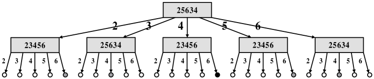
Figure 7: A valid $(2,2)$-ToC $\mathcal{T}$

Definition 4.3 ($\mathbb{B}_{\mathcal{T}}$ for accessing $\mathcal{T}$).

Suppose $\mathcal{T}$ is a valid $(n,d)$-ToC. The input to $\mathbb{B}_{\mathcal{T}}$ is a point $\mathbf{q}$ from $(\mathbb{J}_{n})^{d}$ (defining the name of a leaf $u$ in $\mathcal{T}$). Let $h=\mbox{{\sf height}}\left(\mbox{{\sf head}}\left(u\right)\right)$. If $u$ is the tail of $\mathcal{T}$, i.e., $h=d$, then $\mathbb{B}_{\mathcal{T}}=\mathcal{T}$. Otherwise, let $v_{1}=\mbox{{\sf head}}\left(u\right)$ and let $v$ be the parent of $v_{1}$. Note that $v_{1}$ is the $q_{d-h}^{th}$-successor of $v$. Let $\mathcal{T}_{1}$ be the tree rooted at $v_{1}$. As $u\neq\mbox{{\sf tail}}\left(v\right)$, $\phi_{C_{v}}(q_{d-h})$ is defined and let $\mathcal{T}_{2}$ be the subtree rooted the $\phi_{C_{v}}(q_{d-h})^{th}$-successor of $v$. Then, $\mathbb{B}_{\mathcal{T}}(\mathbf{q})=(h,\phi_{C_{v}}(q_{d-h}),\mathcal{T}_{1},\mathcal{T}_{2})$.

We now define our final search problem Name-the-Tail, on a valid $(n,d)$-ToC. The search problem NT^d is: Given a valid $(n,d)$-ToC $\mathcal{T}^{*}$ accessible by $\mathbb{B}_{\mathcal{T}^{*}}$, find the name of its tail. We will prove Theorem 4.4 in Section 4.3. Below, we prove Theorem 4.5 to reduce $\text{\sf NT}^{d}$ to $\text{\sf ES}^{d}$.

Theorem 4.4 (Complexity of $\text{\sf NT}^{d}$).

For all sufficiently large $n$,

$$\text{\sf RQ}_{\text{\sf NT}}^{d}(n)\hskip 1.70709pt\geq\hskip 1.70709pt\frac{1}{2}\left(\frac{n}{2\cdot 24^{d}}\right)^{d}.$$

Theorem 4.5 (From $\text{\sf NT}^{d}$ to $\text{\sf ES}^{d}$).

For all $d\geq 1$, $\text{\sf RQ}_{\text{\sf NT}}^{d}(n)\leq\text{\sf RQ}_{\text{\sf ES}}^{d}(4n+4)$.

Proof.

We need to build a $d$-non-repeating string from a valid $(n,d)$-ToC $\mathcal{T}$. In fact, we will construct two strings $S[\mathcal{T}]$ and $Q[\mathcal{T}]$ over $\mathbb{Z}_{4n+4}$, each has length $\Theta(n^{d})\cdot d$. $S[\mathcal{T}]$ starts with $\mathbf{s}_{d}$ and ends with $\mathcal{F}(\mbox{{\sf name}}\left(\mbox{{\sf tail}}\left(\mathcal{T}\right)\right))\in\mathbb{Z}^{d}$ while $Q[\mathcal{T}]$ starts with $\mathcal{F}(\mbox{{\sf name}}\left(\mbox{{\sf tail}}\left(\mathcal{T}\right)\right))$ and ends with $\mathbf{s}_{d}$, where for $\mathbf{p}\in\mathbb{Z}^{d}$ $\mathcal{F}(\mathbf{p})=(2p_{1},...,2p_{d-1},2p_{d}-1)$ and $\mathbf{s}_{d}\in\mathbb{Z}^{d}$ defined to be $s_{1}=1$, and $\mathbf{s}_{d}=(2,...,2,1)$ for $d>1$.

For any two strings $S_{1}=a_{1}...a_{k}$ and $S_{2}=b_{1}...b_{t}$, let $S_{1}\circ S_{2}=a_{1}...a_{k}b_{1}...b_{t}$. For $d\geq 1$, if $a_{k-d+i}=b_{i}$ for all $1\leq i\leq d$, then let $S_{1}\circ_{d}S_{2}=a_{1}...a_{k}b_{d+1}...b_{t}$. Given a string $S$ over $\mathbb{Z}$ of length $k\cdot d$, we write $S$ as $\mathbf{u}_{1}...\mathbf{u}_{k}$ with $\mathbf{u}_{i}\in\mathbb{Z}^{d}$. Let $\mbox{{\sf insert}}_{d}\left(S,t\right)=\mathbf{u}_{1}\circ t\circ\mathbf{u}_{2}\circ t...\mathbf{u}_{k-1}\circ t\circ\mathbf{u}_{k}$.

We use the following recursive procedure. Let $r$ be the root of $\mathcal{T}$. Assume $C_{r}=a_{1}...a_{2n+1}$. When $d=1$, we set $S[\mathcal{T}]=1b_{1}b_{2}...b_{2n+1}$ and $Q[\mathcal{T}]=b_{2n+1}...b_{2}b_{1}1$, where $b_{i}=2a_{i}-1$. When $d\geq 2$,

1. let $\mathcal{T}_{i}$ be the subtree of $\mathcal{T}$ rooted at the $a_{i}^{th}$-successor of $r$ and let $\mathbf{p}_{i}\in(\mathbb{F}_{n})^{d-1}$ be the name of the tail of $\mathcal{T}_{i}$ given by $\mathcal{T}_{i}$ (not by $\mathcal{T}$).

2. for every odd $i\in[1:2n+1]$, set $S^{\prime}_{i}=\mbox{{\sf insert}}_{d-1}\left(S[\mathcal{T}_{i}],2a_{i}\right)$ (which starts with $\mathbf{s}_{d-1}$ and ends with $\mathcal{F}(\mathbf{p}_{i})$) and for every even $i\in[1:2n+1]$ set $S^{\prime}_{i}=\mbox{{\sf insert}}_{d-1}\left(Q[\mathcal{T}_{i}],2a_{i}\right)$ (which starts with $\mathcal{F}(\mathbf{p}_{i})$ and ends with $\mathbf{s}_{d-1}$); $S[\mathcal{T}]=\mathbf{s}_{d}\circ_{d-1}S_{1}^{\prime}\circ_{d-1}S_{2}^{\prime}\circ_{d-1}S_{3}^{\prime}\circ_{d-1}...\circ_{d-1}S_{2n}^{\prime}\circ_{d-1}S_{2n+1}^{\prime}$;

3. for every odd $i\in[1:2n+1]$, set $Q^{\prime}_{i}=\mbox{{\sf insert}}_{d-1}\left(Q[\mathcal{T}_{i}],2a_{i}\right)$ (which starts with $\mathcal{F}(\mathbf{p}_{i})$ and ends with $\mathbf{s}_{d-1}$) and for every even $i\in[1:2n+1]$, set $Q^{\prime}_{i}=\mbox{{\sf insert}}_{d-1}\left(S[\mathcal{T}_{i}],2a_{i}\right)$ (which starts with $\mathbf{s}_{d-1}$ and ends with $\mathcal{F}(\mathbf{p}_{i})$); $Q[\mathcal{T}]=(2a_{2n+1})\circ Q^{\prime}_{2n+1}\circ_{d-1}Q^{\prime}_{2n}\circ_{d-1}...\circ_{d-1}Q^{\prime}_{2}\circ_{d-1}Q^{\prime}_{1}\circ\mathbf{s}_{d}.$

The two strings for the example in Figure 7 above are:

$$S[\mathcal{T}]=\raisebox{2.75555pt}{2}\hskip 0.56917pt1\hskip 0.56917pt\raisebox{2.75555pt}{4}\hskip 0.56917pt3\hskip 0.56917pt\raisebox{2.75555pt}{4}\hskip 0.56917pt5\hskip 0.56917pt\raisebox{2.75555pt}{4}\hskip 0.56917pt7\hskip 0.56917pt\raisebox{2.75555pt}{4}\hskip 0.56917pt9\hskip 0.56917pt\raisebox{2.75555pt}{4}\hskip 0.56917pt11\hskip 0.56917pt\raisebox{2.75555pt}{10}\hskip 0.56917pt9\hskip 0.56917pt\raisebox{2.75555pt}{10}\hskip 0.56917pt7\hskip 0.56917pt\raisebox{2.75555pt}{10}\hskip 0.56917pt5\hskip 0.56917pt\raisebox{2.75555pt}{10}\hskip 0.56917pt3\hskip 0.56917pt\raisebox{2.75555pt}{10}\hskip 0.56917pt1\hskip 0.56917pt\raisebox{2.75555pt}{12}\hskip 0.56917pt3\hskip 0.56917pt\raisebox{2.75555pt}{12}\hskip 0.56917pt9\hskip 0.56917pt\raisebox{2.75555pt}{12}\hskip 0.56917pt11\hskip 0.56917pt\raisebox{2.75555pt}{12}\hskip 0.56917pt5\hskip 0.56917pt\raisebox{2.75555pt}{12}\hskip 0.56917pt7\hskip 0.56917pt\raisebox{2.75555pt}{6}\hskip 0.56917pt5\hskip 0.56917pt\raisebox{2.75555pt}{6}\hskip 0.56917pt11\hskip 0.56917pt\raisebox{2.75555pt}{6}\hskip 0.56917pt9\hskip 0.56917pt\raisebox{2.75555pt}{6}\hskip 0.56917pt3\hskip 0.56917pt\raisebox{2.75555pt}{6}\hskip 0.56917pt1\hskip 0.56917pt\raisebox{2.75555pt}{8}\hskip 0.56917pt3\hskip 0.56917pt\raisebox{2.75555pt}{8}\hskip 0.56917pt5\hskip 0.56917pt\raisebox{2.75555pt}{8}\hskip 0.56917pt7\hskip 0.56917pt\raisebox{2.75555pt}{8}\hskip 0.56917pt9\hskip 0.56917pt\raisebox{2.75555pt}{8}\hskip 0.85355pt11$$

$$Q[\mathcal{T}]=\raisebox{2.75555pt}{8}\hskip 0.56917pt11\hskip 0.56917pt\raisebox{2.75555pt}{8}\hskip 0.56917pt9\hskip 0.56917pt\raisebox{2.75555pt}{8}\hskip 0.56917pt7\hskip 0.56917pt\raisebox{2.75555pt}{8}\hskip 0.56917pt5\hskip 0.56917pt\raisebox{2.75555pt}{8}\hskip 0.56917pt3\hskip 0.56917pt\raisebox{2.75555pt}{8}\hskip 0.56917pt1\hskip 0.56917pt\raisebox{2.75555pt}{6}\hskip 0.56917pt3\hskip 0.56917pt\raisebox{2.06668pt}{6}\hskip 0.56917pt9\hskip 0.56917pt\raisebox{2.75555pt}{6}\hskip 0.56917pt11\hskip 0.56917pt\raisebox{2.75555pt}{6}\hskip 0.56917pt5\hskip 0.56917pt\raisebox{2.75555pt}{6}\hskip 0.56917pt7\hskip 0.56917pt\raisebox{2.75555pt}{12}\hskip 0.56917pt5\hskip 0.56917pt\raisebox{2.75555pt}{12}\hskip 0.56917pt11\hskip 0.56917pt\raisebox{2.75555pt}{12}\hskip 0.56917pt9\hskip 0.56917pt\raisebox{2.75555pt}{12}\hskip 0.56917pt3\hskip 0.56917pt\raisebox{2.75555pt}{12}\hskip 0.56917pt1\hskip 0.56917pt\raisebox{2.75555pt}{10}\hskip 0.56917pt3\hskip 0.56917pt\raisebox{2.75555pt}{10}\hskip 0.56917pt5\hskip 0.56917pt\raisebox{2.75555pt}{10}\hskip 0.56917pt7\hskip 0.56917pt\raisebox{2.75555pt}{10}\hskip 0.56917pt9\hskip 0.56917pt\raisebox{2.75555pt}{10}\hskip 0.56917pt11\hskip 0.56917pt\raisebox{2.75555pt}{4}\hskip 0.56917pt9\hskip 0.56917pt\raisebox{2.75555pt}{4}\hskip 0.56917pt7\hskip 0.56917pt\raisebox{2.75555pt}{4}\hskip 0.56917pt5\hskip 0.56917pt\raisebox{2.75555pt}{4}\hskip 0.56917pt3\hskip 0.56917pt\raisebox{2.75555pt}{4}\hskip 0.85355pt1\hskip 0.85355pt\raisebox{2.75555pt}{2}\hskip 0.85355pt1$$

The correctness of our construction can be established using the next two lemmas. ∎

Lemma 4.6 (Non-Repeating).

If $\mathcal{T}$ is a valid $(n,d)$-ToC, then both $S[\mathcal{T}]$ and $Q[\mathcal{T}]$ are $d$-non-repeating.

Proof.

We prove the lemma by induction on $d$. The base case when $d=1$ is trivial.

Assume $d>1$ and also inductively that the statement is true for $d-1$. Suppose for the sake of contradiction that $S^{\prime}=a_{1}a_{2}...a_{d}\in\mathbb{Z}_{4n+4}^{d}$ appears in $S[\mathcal{T}]$ more than once. Note that exactly one symbol in $S^{\prime}$, say $a_{t}$, is odd. Let $k\in[1:d]$ be the following integer: if $t=d$, then $k=1$; otherwise, $k=t+1$.

First, if $a_{k}=2$, then $S^{\prime}$ appears in $S[\mathcal{T}]$ implies $(a_{1},a_{2},...,a_{d})=\mathbf{s}_{d}$. But such $S^{\prime}$ only appears in $S[\mathcal{T}]$ once, which contradicts with the assumption.

Otherwise, let $S^{\prime\prime}\in\mathbb{Z}_{4n+4}^{d-1}$ be the string obtained by removing $a_{k}$ from $S^{\prime}$, then: if $a_{k}/2$ is odd, then $S^{\prime\prime}$ appears in $Q[\mathcal{T}_{a_{k}/2}]$ more than once; otherwise, $S^{\prime\prime}$ appears in $S[\mathcal{T}_{a_{k}/2}]$ more than once, which contradicts with the inductive hypothesis.

The proof for string $Q[\mathcal{T}]$ is similar. ∎

Lemma 4.7 (Asking $\mathbb{B}_{\mathcal{T}}$).

Suppose $\mathcal{T}$ is a valid $(n,d)$-ToC and $S=S[\mathcal{T}]$ and $Q=Q[\mathcal{T}]$. For any $\mathbf{u}\in\mathbb{Z}^{d}_{4n+4}$, we can compute $\mathbb{B}_{S}(\mathbf{u})$ and $\mathbb{B}_{Q}(\mathbf{u})$ by querying $\mathbb{B}_{\mathcal{T}}$ at most once.

Proof.

We need the following two propositions. Proposition 4.9 can be proved by mathematical induction on $d$.

Proposition 4.8 (Vectors not in $S$ and $Q$).

Let $V_{1}=\{2,4,...,4n+4\}^{d-1}\times\{1,3,...,4n+3\}$ and $V_{k}=\{2,4,...,4n+4\}^{k-2}\times\{1,3,...,4n+3\}\times\{2,4,...,4n+4\}^{d-k+1}$ for $2\leq k\leq d$. If $\mathbf{u}\notin\cup_{k}V_{k}$ then $\mathbf{u}$ neither appears in $S$ nor in $Q$.

Proposition 4.9 (All the same).

Let $\mathcal{T}$ and $\mathcal{T}^{\prime}$ two valid $(n,d)$-ToCs. If $\mathbf{u}\in\cup_{k}V_{k}$ and $u_{i}=1$ or $u_{i}=2$ for some $1\leq i\leq d$, then $\mathbb{B}_{S[\mathcal{T}]}(\mathbf{u})=\mathbb{B}_{S[\mathcal{T}^{\prime}]}(\mathbf{u})$ and $\mathbb{B}_{Q[\mathcal{T}]}(\mathbf{u})=\mathbb{B}_{Q[\mathcal{T}^{\prime}]}(\mathbf{u})$.

We first consider two simple cases for which we don’t even need to query $\mathbb{B}_{\mathcal{T}}$.

1. When $\mathbf{u}\notin\cup_{k}V_{k}$, by Proposition 4.8, $\mathbb{B}_{S[\mathcal{T}]}(\mathbf{u})=\mathbb{B}_{Q[\mathcal{T}]}(\mathbf{u})=(\text{``no'',``no''})$;

2. When $\mathbf{u}\in\cup_{k}V_{k}$ and $u_{i}=1$ or $u_{i}=2$ for some $1\leq i\leq d$, by Proposition 4.9, we can compute $\mathbb{B}_{S}(\mathbf{u})$ and $\mathbb{B}_{Q}(\mathbf{u})$ from the valid $(n,d)$-tree in which every connector is generated by the identity permutation from $\{1,\dotsc,n\}$ to $\{1,\dotsc,n\}$.

Now we can assume $\mathbf{u}\in\cup_{k}U_{k}$ where $U_{1}=\{4,6,...,4n+4\}^{d-1}\times\{3,5,...,4n+3\}$ and $U_{k}=\{4,6...,4n+4\}^{k-2}\times\{3,5,...,4n+3\}\times\{4,6,...,4n+4\}^{d-k+1}$ for $2\leq k\leq d$. First note that there is exactly one odd entry in $\mathbf{u}$. If $\mathbf{u}\in U_{k}$ then let $\mathbf{u}^{\prime}$ be the string obtained from $\mathbf{u}$ by $k-1$ left-rotations. Not the last entry of $\mathbf{u}^{\prime}$ is odd. Let $\mathbf{q}$ be the vector in $(\mathbb{J}_{n})^{d}$ where $q_{i}=u^{\prime}_{i}/2$ for $1\leq i\leq d-1$ and $q_{d}=(u^{\prime}_{d}+1)/2$. We now prove a stronger statement which implies that $\mathbb{B}_{S}(\mathbf{u})$ and $\mathbb{B}_{Q}(\mathbf{u})$ can be computed from $\mathbb{B}_{\mathcal{T}}(\mathbf{q})$.

For all $\mathbf{q}\in(\mathbb{J}_{n})^{d}$, we can determine $\mathbb{B}_{S}(\mathbf{u}_{i})$ and $\mathbb{B}_{Q}(\mathbf{u}_{i})$ from $\mathbb{B}_{\mathcal{T}}(\mathbf{q})$, where $\mathbf{u}_{k}$ is the vector in $U_{k}$ obtained from $\mathcal{F}(\mathbf{q})$ by $k-1$ right rotations, for $1\leq k\leq d$.

If $\mathbb{B}_{\mathcal{T}}(\mathbf{q})=\mathcal{T}$, the statement is clearly true. Otherwise, assuming $\mathbb{B}_{\mathcal{T}}(\mathbf{q})\not=\mathcal{T}$, we prove the statement by induction on $d$. The base case when $d=1$ is trivial. For $d\geq 2$, let $\mathbf{q}^{\prime}=(q_{2},q_{3},...,q_{d})$ and let $\mathbf{v}_{k}$ be the vector generated from $\mathcal{F}(\mathbf{q}^{\prime})$ by $k-1$ right rotations, for $1\leq k\leq d-1$. Let $\mathcal{T}^{\prime}$ be the subtree of $\mathcal{T}$ rooted the $q_{1}$-successor of the root of $\mathcal{T}$. As $\mathbb{B}_{\mathcal{T}^{\prime}}(\mathbf{q}^{\prime})$ is contained in $\mathbb{B}_{\mathcal{T}}(\mathbf{q})$, we can determine $\mathbb{B}_{S[\mathcal{T}^{\prime}]}(\mathbf{v}_{i})$ and $\mathbb{B}_{Q[\mathcal{T}^{\prime}]}(\mathbf{v}_{i})$ for using our inductive hypothesis, from which, we will show below, we can determine $\mathbb{B}_{S}(\mathbf{u}_{i})$ and $\mathbb{B}_{Q}(\mathbf{u}_{i})$.

We will only prove the case for $\mathbb{B}_{S}(\mathbf{u}_{i})$ when $q_{1}$ is even. All other cases are similar.

Note that the first entry of $\mathbf{v}_{i}$ is not 2, so for all $1\leq i\leq d-1$, $\mathbb{B}_{S[\mathcal{T}^{\prime}]}(\mathbf{v}_{i})\not=(\text{``no''},a)$. Also, for $i>1$ the last entry of $\mathbf{v}_{i}$ is even, so, $\mathbb{B}_{S[\mathcal{T}^{\prime}]}(\mathbf{v}_{i})$ $\not=(a,\text{``no''})$. Therefore, for all $i\in[2:d-1]$, $\mathbb{B}_{S}(\mathbf{u}_{i})=\mathbb{B}_{S[\mathcal{T}^{\prime}]}(\mathbf{v}_{i})$. For $i=1$ or $d$, if $\mathbb{B}_{S[\mathcal{T}^{\prime}]}(\mathbf{v}_{1})=(\text{``no''},\text{``no''})$, then $\mathbb{B}_{S}(\mathbf{u}_{i})=(\text{``no''},\text{``no''})$; if $\mathbb{B}_{S[\mathcal{T}^{\prime}]}(\mathbf{v}_{1})=(a,b)$, then $\mathbb{B}_{S}(\mathbf{u}_{1})=(a,2q_{1})$, $\mathbb{B}_{S}(\mathbf{u}_{d})=(2q_{1},b)$; if $\mathbb{B}_{S[\mathcal{T}^{\prime}]}(\mathbf{v}_{1})=(a,\text{``no''})$, letting the second component of $\mathbb{B}_{\mathcal{T}}(\mathbf{q})$ be $r$, then $\mathbb{B}_{S}(\mathbf{u}_{1})=(a,2r)$ and $\mathbb{B}_{S}(\mathbf{u}_{d})=(\text{``no''},\text{``no''})$. ∎

4.2 Knowledge Representation in Algorithms for NT^d and a Key Lemma

An algorithm for NT^d tries to learn about the connectors in $\mathcal{T}^{*}$ by repeatedly querying its leaves. To capture its intermediate knowledge about this $\mathcal{T}^{*}$, we introduce a notion of partial connectors.

Let $\mathbf{\sigma}=[\sigma(1),...,\sigma(k)]$ be an array of distinct elements from $\{0,1,...n\}$. Then, $\mathbf{\sigma}$ defines a string $S_{\sigma(1)}\circ...\circ S_{\sigma(k)}$, referred to as a connecting segment. Recall $S_{0}=2,S_{1}=3\circ 4,...S_{n}=(2n+1)\circ(2n+2)$. A partial connector over $\mathbb{J}_{n}$ is then a set $\mathcal{C}$ of connecting segments such that each $j\in\mathbb{J}_{n}$ is contained in exactly one segment in $\mathcal{C}$ and 2 is the first element of the segment containing it. If $\mathcal{C}$ has $n+1$ segments, that is, $\mathcal{C}=\{2,3\circ 4,...,(2n+1)\circ(2n+2)\}$, then $\mathcal{C}$ is called an empty connector. We say a connector $C$ is consistent with a partial connector $\mathcal{C}$ if every segment in $\mathcal{C}$ is a substring of $C$.

Let $r[\mathcal{C}]$ be the last symbol of the segment in $\mathcal{C}$ that starts with 2. Let $L[\mathcal{C}]$ and $R[\mathcal{C}]$, respectively, be the set of first and the last symbols of other segments in $\mathcal{C}$. So, $r[\mathcal{C}]\in\mathbb{F}_{n}\cup\{2\}$, $L[\mathcal{C}]\subset\mathbb{O}_{n}$, and $R[\mathcal{C}]\subset\mathbb{F}_{n}$. Also, $|\hskip 1.13791ptL[\mathcal{C}]\hskip 1.13791pt|=|\hskip 1.13791ptR[\mathcal{C}]\hskip 1.13791pt|$. If $2\neq r[\mathcal{C}]$, we use $\phi_{\mathcal{C}}(2)$ to denote its right neighbor. Note that each $s\in\mathbb{J}_{n}-L[\mathcal{C}]\cup R[\mathcal{C}]\cup\{r[\mathcal{C}],2\}$ has two neighbors in $\mathcal{C}$. If $s$ is even, we will use $\phi_{\mathcal{C}}(s)$ to denote its right neighbor and if $s$ is odd, we use $\phi_{\mathcal{C}}(s)$ to denote its left neighbor.

Initially, the knowledge of an algorithm for NT^d can be viewed as a tree $\mathcal{T}$ of empty connectors. At each round, the algorithm chooses a query point $\mathbf{q}$ and asks for $\mathbb{B}_{\mathcal{T}^{*}}(\mathbf{q})$, which may connect some segments in the partial connectors. So $\mathcal{T}$ is updated. The algorithm succeeds when every partial connector becomes a connector and $\mathcal{T}$ grows into $\mathcal{T}^{*}$.

So, at intermediate steps, the knowledge of the algorithm can be expressed by a tree $\mathcal{T}$ of partial connectors.

Definition 4.10 (Valid Tree of Partial Connectors).

An $(n,d)$-ToPC $\mathcal{T}$ is a tree $T_{n,d}$ in which each internal node $v$ is associated with a partial connector $\mathcal{C}_{v}$ over $\mathbb{J}_{n}$.

$\mathcal{T}$ is a valid $(n,d)$-ToPC if for each internal node $v\in T_{n,d}$ whose children are not leaves, its partial connector $\mathcal{C}_{v}$ at $v$ satisfies the following condition: For each pair $s,t\in\mathbb{J}_{n}$ with $\phi_{\mathcal{C}_{v}}(s)=t$, the tree $\mathcal{T}_{s}$ rooted at the $s^{th}$-successor $v_{s}$ and the tree $\mathcal{T}_{t}$ rooted at the $t^{th}$-successor $v_{t}$ of $v$ are both valid ToCs, and $\mbox{{\sf name}}\left(\mbox{{\sf tail}}\left(v_{s}\right)\right)$ in $\mathcal{T}_{s}$ and $\mbox{{\sf name}}\left(\mbox{{\sf tail}}\left(v_{t}\right)\right)$ in $\mathcal{T}_{t}$ are the same.

A valid $(n,d)$-ToC $\mathcal{T}^{*}$ is consistent with a valid $(n,d)$-ToPC $\mathcal{T}$, denoted by $\mathcal{T}\models\mathcal{T}^{*}$, if for every internal node, its connector in $\mathcal{T}^{*}$ is consistent with its (partial) connector in $\mathcal{T}$.

A partial connector $\mathcal{C}$ is a $\beta$-partial connector for $0<\beta<1$ if the number of segments in $\mathcal{C}$ is at least $(1-\beta)n+1$. To simplify our proof, we will relax our oracle $\mathbb{B}_{\mathcal{T}^{*}}$ to sometime provide more information to the algorithm than being asked so that the $\mathcal{T}$ it maintains always satisfies the conditions of the following definition:

Definition 4.11 (Valid $(n,d,\beta)$-ToPC).

A valid $(n,d)$-ToPC $\mathcal{T}$ is a valid $(n,d,\beta)$-ToPC if its root has a $\beta$-partial connector, Moreover, for each internal node $v\in T_{n,d}$ whose children are not leaves, if the partial connector $\mathcal{C}_{v}$ at $v$ is a $\beta$-partial connector, then it satisfies the following condition: The $s^{th}$-successor of $v$, for each $s\in L[\mathcal{C}]\cup R[\mathcal{C}]\cup\{r[\mathcal{C}]\}$, has a $\beta$-partial connector.

Key to our analysis is Lemma 4.12 below, stating that every valid $(n,d,\beta)$-ToPC has a large number of consistent valid $(n,d)$-ToCs, and moreover, the names of the tails of these ToCs are nearly-uniformly distributed. Let $\mathcal{F}[\mathcal{T}]=\{\hskip 1.13791pt\mbox{{\sf name}}\left(\mbox{{\sf tail}}\left(\mathcal{T}^{*}\right)\right)\big{|}\hskip 2.84544pt\mathcal{T}\models\mathcal{T}^{*}\hskip 1.13791pt\}.$ Also, for each $\mathbf{p}\in(\mathbb{F}_{n})^{d}$, let $N[\mathcal{T},\mathbf{p}]=|\hskip 1.42271pt\{\hskip 1.13791pt\mathcal{T}^{*}\hskip 1.70709pt\big{|}\hskip 2.84544pt\mathcal{T}\models\mathcal{T}^{*}\ \text{and}\ \mbox{{\sf name}}\left(\mbox{{\sf tail}}\left(\mathcal{T}^{*}\right)\right)=\mathbf{p}\hskip 1.13791pt\}\hskip 1.42271pt|$.

Lemma 4.12 (Key Lemma).

For $d\geq 1$ and $\beta\in[0,24^{-d}]$, $|\hskip 1.13791pt\mathcal{F}[\mathcal{T}]\hskip 0.28436pt|\geq(\hskip 0.56917pt(1-\beta)n\hskip 0.56917pt)^{d}$ for each valid $(n,d,\beta)$-ToPC $\mathcal{T}$. Let $\alpha_{1}(\beta)=1$. Then, for all $\mathbf{p}_{1},\mathbf{p}_{2}\in\mathcal{F}[\mathcal{T}]$,

$$\frac{1}{\alpha_{d}(\beta)}\hskip 1.42271pt\leq\hskip 1.42271pt\frac{N[\mathcal{T},\mathbf{p}_{1}]}{N[\mathcal{T},\mathbf{p}_{2}]}\hskip 1.42271pt\leq\hskip 1.42271pt\alpha_{d}(\beta),\quad\mbox{ where }\quad\alpha_{d}(\beta)=\frac{\left(\alpha_{d-1}\left(\beta\right)\right)^{7}}{(2\left(1-\beta\right)^{d-1}-1)^{3}},\mbox{ for $d\geq 2$}.\vspace{0.1cm}$$ (1)

Proof.

When $d=1$, let $\mathcal{C}$ be the only partial connector in $\mathcal{T}$. Clearly, $\mathcal{F}[\mathcal{T}]=R[\mathcal{C}]$. Thus, in this case the lemma is true. We will also use this case as the base of the induction below. When $d\geq 2$, let $\mathcal{C}$ be the partial connector of the root. For each $k\in\mathbb{J}_{n}$, let $\mathcal{T}_{k}$ be the subtree of the $k^{{th}}$-successor of the root. Below, we will prove by induction on $d$ that (1) and (**) $\mathcal{F}[\mathcal{T}]=\cup_{k\in R[\mathcal{C}]}(k\circ\mathcal{F}[\mathcal{T}_{k}]\hskip 1.70709pt)$ are true for all $d$. Note that (**) and the first condition of Definition 4.11 imply that $|\hskip 1.13791pt\mathcal{F}[\mathcal{T}]\hskip 0.28436pt|\geq(\hskip 0.56917pt(1-\beta)n\hskip 0.56917pt)^{d}.$

Let $\mathcal{C}=\{\hskip 1.13791ptY_{0},Y_{1},Y_{2},...,Y_{m}\hskip 1.13791pt\}$ be the $\beta$-partial connector at the root of $\mathcal{T}$; assume $Y_{0}$ is the segment starting with $2$. We use $r_{i}$ and $t_{i}$, respectively, to denote the ending and starting symbols of $Y_{i}$. For each $k\in\{\hskip 1.13791ptr_{0},...,r_{m},t_{1},...,t_{m}\hskip 1.13791pt\}$, let $\mathcal{T}_{k}$ denote the $(n,d-1,\beta)$-ToPC at the $k^{{th}}$-successor of the root. For each pair $(i,j)\in[0:m]\times[1:m]$ with $i\not=j$, we define

$$N_{i,j}=\sum_{\mathbf{p}\in\mathcal{F}[\mathcal{T}_{r_{i}}]\cap\mathcal{F}[\mathcal{T}_{t_{j}}]}N[\mathcal{T}_{r_{i}},\mathbf{p}]\cdot N[\mathcal{T}_{t_{j}},\mathbf{p}].$$

Inductively, (1) and (**) hold for all $d^{\prime}<d$. As a result, we have $|\hskip 1.13791pt\mathcal{F}[\mathcal{T}_{k}]\hskip 1.13791pt|\geq((1-\beta)n)^{d-1}$ for every $k\in\{\hskip 0.85355ptr_{0},...r_{m},t_{1},...t_{m}\hskip 0.85355pt\}$. Thus,

$$|\hskip 1.13791pt\mathcal{F}[\mathcal{T}_{r_{i}}]\cap\mathcal{F}[\mathcal{T}_{t_{j}}]\hskip 1.13791pt|=|\hskip 1.13791pt\mathcal{F}[\mathcal{T}_{r_{i}}]\hskip 1.13791pt|+|\hskip 1.13791pt\mathcal{F}[\mathcal{T}_{t_{j}}]\hskip 1.13791pt|-|\hskip 1.13791pt\mathcal{F}[\mathcal{T}_{r_{i}}]\cup\mathcal{F}[\mathcal{T}_{t_{j}}]\hskip 1.13791pt|\geq(2(1-\beta)^{d-1}-1)\hskip 1.13791ptn^{d-1}>0,\vspace{0.08cm}$$

because $\beta\leq 24^{-d}$. By the inductive hypothesis, we have $N_{i,j}>0$, for all $(i,j)\in[0:m]\times[1:m]$ with $i\not=j$.

To show (**), it suffices to prove that $N[\mathcal{T},\mathbf{p}]>0$ if and only if $\mathbf{p}\in\cup_{k\in R[\mathcal{C}]}(k\circ\mathcal{F}[\mathcal{T}_{k}]\hskip 1.70709pt).$ Clearly, $N[\mathcal{T},\mathbf{p}]=0$ for $\mathbf{p}\not\in\cup_{k\in R[\mathcal{C}]}(k\circ\mathcal{F}[\mathcal{T}_{k}]\hskip 1.70709pt).$ So, let us consider $\mathbf{p}\in\cup_{k\in R[\mathcal{C}]}(k\circ\mathcal{F}[\mathcal{T}_{k}]\hskip 1.70709pt).$ Since $p_{1}\in R[\mathcal{C}]$, WLOG, assume $p_{1}=r_{m}$. We use $\mathcal{P}$ to denote the set of permutations $s_{0}s_{1}...s_{m-1}$ over $[0:m-1]$ with $s_{0}=0$. Then

$$N[\mathcal{T},\mathbf{p}]=\sum_{s_{0}s_{1}...s_{m-1}\in\mathcal{P}}\left(\left(\prod_{i=0}^{m-2}N_{s_{i},s_{i+1}}\right)\cdot N_{s_{m-1},m}\cdot N\big{[}\mathcal{T}_{r_{m}},(p_{2},p_{3},...,p_{d})\big{]}\hskip 0.85355pt\right).$$

By the inductive hypothesis, every item in the summation above is positive. So $N[\mathcal{T},\mathbf{p}]>0$ and (**) holds for $d$.

Next, to prove (1), consider $\mathbf{p}_{1}\in\mathcal{F}[\mathcal{T}]$ and $\mathbf{p}_{2}\in\mathcal{F}[\mathcal{T}]$. There are two basic cases. When $p_{1,1}=p_{2,1}$, Eqn. (1) follows directly from (4.2) and the inductive hypothesis. When $p_{1,1}\neq p_{2,1}$, without loss of generality, we assume $p_{1,1}=r_{m}$ and $p_{2,1}=r_{m-1}$.

Let $\mathcal{P}_{1}$ denote the set of permutations over $\{0,1,...,m-2,m-1\}$ with $s_{0}=0$ and $\mathcal{P}_{2}$ denote the set of permutations over $\{0,1,...,m-2,m\}$ with $s_{0}=0$. For $P=s_{0}s_{1}...s_{m-1}\in\mathcal{P}_{1}$ , let $\Pi(P)$ be the permutation obtained from $P$ by replacing $m-1$ by $m$. Clearly $\Pi$ is a bijection from $\mathcal{P}_{1}$ to $\mathcal{P}_{2}$. We can write $N[\mathcal{T},\mathbf{p}_{1}]$ and $N[\mathcal{T},\mathbf{p}_{2}]$ as two summations:

$$N[\mathcal{T},\mathbf{p}_{1}]=\sum_{P\in\mathcal{P}_{1}}N_{1}(P),\ \ \ \ \text{and}\ \ \ \ N[\mathcal{T},\mathbf{p}_{2}]=\sum_{P\in\mathcal{P}_{1}}N_{2}(\Pi(P)),$$

where $N_{1}(P)$ and $N_{2}(\Pi(P))$ are given by similar terms as in (4.2).

We now prove for every $P\in\mathcal{P}_{1}$, $(N_{1}(P)/N_{2}(\Pi(P))\leq\alpha_{d}(\beta)$. Let $P=s_{0}s_{1}...s_{m-1}$ where $s_{k}=m-1$ for some $1\leq k\leq m-1$. If $k<m-1$, then we expand $N_{1}(P)$ and $N_{2}(\Pi(P))$ as:

$$\frac{N_{1}(P)}{N_{2}(\Pi(P))}=\frac{N_{s_{k-1},m-1}\cdot N_{m-1,s_{k+1}}\cdot N_{s_{m-1},m}\cdot N[\mathcal{T}_{r_{m}},(p_{1,2},p_{1,3},...,p_{1,d})]}{N_{s_{k-1},m}\cdot N_{m,s_{k+1}}\cdot N_{s_{m-1},m-1}\cdot N[\mathcal{T}_{r_{m-1}},(p_{2,2},p_{2,3},...,p_{2,d})]}.\vspace{0.03cm}$$

It then follows from the application of our inductive hypothesis to the straightforward expansion of terms $N_{i,j}$ that $N_{1}(P)/N_{2}(\Pi(P))\leq\alpha_{d}(\beta)$.

Similarly, we can establish the same bound for the case when $k=m-1$. ∎

4.3 The Randomized Query Complexity of NT^d

By querying every leaf, one can solve any instance of NT^d with $n^{d}$ queries. Below, we prove Theorem 4.4 by showing $\text{\sf RQ}_{\text{\sf NT}}^{d}(n)=(\Omega(n))^{d}$. We first relax $\mathbb{B}_{\mathcal{T}^{*}}$ by extending it to $(\mathbb{J}_{n})^{m}$ for $m\in[1:d]$.

Definition 4.13 (Relaxation of $\mathbb{B}_{\mathcal{T}^{*}}$).

Suppose $\mathcal{T}^{*}$ is a valid $(n,d)$-ToC and $\mathbf{q}\in(\mathbb{J}_{n})^{m}$. Let $v$ be the node with $\mbox{{\sf name}}\left(v\right)=q_{1}q_{2}...q_{m}$. Let $\mathbf{q}^{\prime}=\mbox{{\sf name}}\left(\mbox{{\sf tail}}\left(v\right)\right)\in(\mathbb{J}_{n})^{d}$ (in tree $\mathcal{T}^{*}$). Then, $\mathbb{B}_{\mathcal{T}^{*}}(\mathbf{q})=\mathbb{B}_{\mathcal{T}^{*}}(\mathbf{q}^{\prime})$.

 

Query-and-Update$(\mathcal{T},\mathbf{q})$, where $\mathbf{q}\in(\mathbb{J}_{n})^{d}$

 

0 :	if $\mathcal{T}$ has complete information of $\mathbf{q}$ then return;
1 :	if  $\exists\ 0\leq i\leq d-1:\big{|}\hskip 0.56917ptR[\mathcal{C}_{i}]\hskip 1.13791pt\big{|}=(1-\beta_{d})n$ then
2 :	set $m$ be the smallest of such $i$ ($m\in[0:d-1]$)
3 :	else set $m=d$
4 :	if $m=0$ then set $\mathcal{T}=\mathcal{T}^{*}$  { and $I=1$ }
5 :	else Update$\hskip 1.70709pt(\mathcal{T},(q_{1},q_{2},...,q_{m}),m)$

 

Update$(\mathcal{T},\mathbf{q},m)$, where $\mathbf{q}\in(\mathbb{J}_{n})^{m}$ and $1\leq m\leq d$

 

6 :	fetch $\mathbb{B}_{\mathcal{T}^{*}}(\mathbf{q})$  { set $A_{m}=A_{m}+1$, $\mathcal{B}_{m}[A_{m}]=0$ and $\mathcal{B}_{m,k}[A_{m}]=0$ }
7 :	if $\mathbb{B}_{\mathcal{T}^{*}}(\mathbf{q})=\mathcal{T}^{*}$ then set $\mathcal{T}=\mathcal{T}^{*}$  { set $\mathcal{B}_{m}[A_{m}]=1$ }
8 :	else [ let $d-m\leq h\leq d-1$ and $r\in\mathbb{J}_{n}$ be the first and second components of $\mathbb{B}_{\mathcal{T}^{*}}(\mathbf{q})$ ]
9 :	set $m^{\prime}=d-h-1$
10 :	$\exists\ Y_{1},Y_{2}\in\mathcal{C}_{m^{\prime}}$: $\{\hskip 1.42271pt\text{the ending symbol of $Y_{1}$, the starting symbol of $Y_{2}$}\hskip 1.42271pt\}=\{\hskip 1.13791ptq_{m^{\prime}+1},r\hskip 1.13791pt\}$
11 :	replace $Y_{1}$ and $Y_{2}$ in $\mathcal{C}_{m^{\prime}}$ by the concatenation of $Y_{1}$ and $Y_{2}$  { set $\mathcal{B}_{m,m^{\prime}}[A_{m}]=1$ }
12 :	let $\mathcal{T}^{\prime}$ and $\mathcal{T}^{\prime\prime}$ be the third and fourth components of $\mathbb{B}_{\mathcal{T}^{*}}(\mathbf{q})$
13 :	replace the subtree of $\mathcal{T}$ rooted at $u_{m^{\prime}+1}$ with $\mathcal{T}^{\prime}$;
14 :	replace the subtree of $\mathcal{T}$ rooted at the $r$-successor of $u_{m^{\prime}}$ with $\mathcal{T}^{\prime\prime}$

 

Figure 8:

Proof (Theorem 4.4).

To apply Yao’s Minimax Principle [32], we consider the distribution $\mathcal{D}$ in which each valid $(n,d)$-ToC $\mathcal{T}^{*}$ is chosen with the same probability. We will prove that the expected query complexity of any deterministic algorithm $\mathcal{A}$ for NT^d over $\mathcal{D}$ is $(\Omega(n))^{d}$. Let $\beta_{d}=24^{-d}$.

Suppose, at a particular step, the current knowledge of $\mathcal{A}$ can be expressed by a valid $(n,d,\beta_{d})$-ToPC $\mathcal{T}$, which is clearly true initially, and $\mathcal{A}$ wants to query $\mathbf{q}\in(\mathbb{J}_{n})^{d}$. Let $u_{0}$ be the root of $\mathcal{T}$ and $u_{i}$ be the node with $\mbox{{\sf name}}\left(u_{i}\right)=q_{1}...q_{i}$. Let $\mathcal{C}_{i}$ be the partial connector at $u_{i}$ in $\mathcal{T}$ and $\mathcal{T}_{i}$ be the subtree of $\mathcal{T}$ of $u_{i}$. There are two cases (1) $\forall i\in[0,d-1]$, $\mathcal{C}_{i}$ is a partial connector and $q_{i+1}\in L[\mathcal{C}_{i}]\cup R[\mathcal{C}_{i}]\cup\{r[\mathcal{C}_{i}]\}$. (2) otherwise. From the definition of $\mathbb{B}_{\mathcal{T}^{*}}$, we can show that in case (2), $\mathbb{B}_{\mathcal{T}^{*}}(\mathbf{q})$ can be answered based on $\mathcal{T}$ only. So, WLOG, we assume $\mathcal{A}$ is smart and never asks unnecessary queries.

In case (1), because $\mathcal{T}$ is a $(n,d,\beta_{d})$-ToPC, $\mathcal{C}_{i}$ is a $\beta_{d}$-partial connector for all $i\in[0,d-1]$. Let $h=\mbox{{\sf height}}\left(\mbox{{\sf head}}\left(\mathbf{q}\right)\right)$. If $h=d$, then $\mathcal{A}$ gets $\mathcal{T}^{*}$. Otherwise, the knowledge gained by querying $\mathbb{B}_{\mathcal{T}^{*}}(\mathbf{q})$ connects two segments in $\mathcal{C}_{d-h-1}$ and replaces the two involved subtrees by the corresponding ones in $\mathbb{B}_{\mathcal{T}^{*}}(\mathbf{q})$. The resulting tree $\mathcal{T}$, however, may no longer be a $(n,d,\beta_{d})$-ToPC, if $|R[\mathcal{C}_{d-h-1}]|=(1-\beta_{d})n$ before the query. We will relax $\mathbb{B}_{\mathcal{T}^{*}}$ to provide $\mathcal{A}$ more information to ensure that the resulting $\mathcal{T}$ remains a valid $(n,d,\beta_{d})$-ToPC. To this end, we consider two subcases: Case (1.a): if $\forall\ i\in[0:d-1]$, $|R[\mathcal{C}_{i}]|>(1-\beta_{d})n$, then $\mathcal{A}$ receives $\mathbb{B}_{\mathcal{T}^{*}}(\mathbf{q})$ as it requested. Case (1.b): if $\exists\ i\in[0:d-1]$ such that $|R[\mathcal{C}_{i}]|=(1-\beta_{d})n$, then let $m=\min\hskip 1.13791pt\{\hskip 1.13791pti:|R[\mathcal{C}_{i}]|=(1-\beta_{d})n\hskip 1.13791pt\}$. Let $\mathbf{q}^{\prime}=(q_{1},...,q_{m})$. Instead of getting $\mathbb{B}_{\mathcal{T}^{*}}(\mathbf{q})$, $\mathcal{A}$ gets $\mathbb{B}_{\mathcal{T}^{*}}(\mathbf{q}^{\prime})$. In this way, the resulting $\mathcal{T}$ remains a valid $(n,d,\beta_{d})$-ToPC. Details of the query-and-update procedure can be found in Figure 8.

We introduce some “analysis variables” to aid our analysis. These variables include: (1) $I\in\{0,1\}$: Initially, $I=0$. If $m=0$ in case (1.b), then we set $I=1$. (2) For each $m\in[1:d]$, $A_{m}\in\mathbb{Z}$, and a set of binary sequences $\mathcal{B}_{m}[...]$ and $\mathcal{B}_{m,k}[...]$, $\forall k\in[0:m-1]$. Initially, $A_{m}=0$, and $\mathcal{B}_{m}$, $\mathcal{B}_{m,k}$ are empty. Each time in case (1.b) when $m>0$, we increase $A_{m}$ by $1$; in case (1.a), we increase $A_{d}$ by $1$. To unify the discussion below, if we have case (1.a), let $m=d$ and $\mathbf{q}^{\prime}=\mathbf{q}$. If $\mathbb{B}_{\mathcal{T}^{*}}(\mathbf{q}^{\prime})=\mathcal{T}^{*}$, we set $\mathcal{B}_{m}[A_{m}]=1$ and $\mathcal{B}_{m,k}[A_{m}]=0$, $\forall k\in[0:m-1]$. Otherwise, if the first component of $\mathbb{B}_{\mathcal{T}^{*}}(\mathbf{q}^{\prime})$ is $d-l$, for $l\in[1:m]$, then set $\mathcal{B}_{m,l-1}[A_{m}]=1$, $\mathcal{B}_{m}[A_{m}]=0$ and $\mathcal{B}_{m,k}[A_{m}]=0$ for all $0\leq k\not=l-1\leq m-1$.

Let $M_{d}=(\beta_{d}n/2)^{d}$. Given a random valid $(n,d)$-ToC $\mathcal{T}^{*}$, if $\mathcal{A}$ stops before making $M_{d}$ queries, let $\{I,A_{m},\mathcal{B}_{m},\mathcal{B}_{m,k}\}$ be the set of analysis variables assigned when $\mathcal{A}$ stops; otherwise, $\{I,A_{m},\mathcal{B}_{m},\mathcal{B}_{m,k}\}$ is assigned after $\mathcal{A}$ makes exactly $M_{d}$ queries. Let $M_{i}=(\beta_{d}n/2)^{i}$. We define a set of binary strings $\{\hskip 1.70709pt\overline{\mathcal{B}}_{m}[1...M_{m}],\overline{\mathcal{B}}_{m,k}[1...M_{m}],\hskip 1.42271pt1\leq m\leq d,\hskip 1.42271pt0\leq k\leq m-1\hskip 1.70709pt\}$ from $\mathcal{B}_{m}$ and $\mathcal{B}_{m,k}$: For every $1\leq i\leq M_{m}$, (I) $\overline{\mathcal{B}}_{m}[i]=\mathcal{B}_{m}[i]$ for $i\leq\min(A_{m},M_{m})$ and $\overline{\mathcal{B}}_{m}[i]=0$ for $A_{m}<i\leq M_{m}$; (II) $\overline{\mathcal{B}}_{m,k}[i]=\mathcal{B}_{m,k}[i]$ for $i\leq\min(A_{m},M_{m})$ and $\overline{\mathcal{B}}_{m,k}[i]=0$ $A_{m}<i\leq M_{m}$.

Let $\left[A\right]$ denote that an event $A$ is true. Let $\mbox{{\rm NOT-YET-FOUND}}\left(\mathcal{T}^{*}\right)$ be the event that $\mathcal{A}$ hasn’t found the tail of $\mathcal{T}^{*}$ after making $M_{d}$ queries. Let ${B}_{m}$, ${B}_{m,k}$, $\overline{B}_{m}$ and $\overline{B}_{m,k}$ denote the number of $1$’s in ${\mathcal{B}}_{m}$, ${\mathcal{B}}_{m,k}$, $\overline{\mathcal{B}}_{m}$ and $\overline{\mathcal{B}}_{m,k}$, respectively. Then, $\left[\mbox{{\rm NOT-YET-FOUND}}\left(\mathcal{T}^{*}\right)\right]$ if and only if $[I=0\mbox{ and}$ $B_{m}=0,\forall m\in[1:d]]$. The theorem directly follows from Lemmas 4.14 below. ∎

Lemma 4.14.

Let $A$ denote the following event,

$$A=\left(\hskip 1.42271pt\overline{B}_{m}=0\mbox{ and }\overline{B}_{m,k}\leq\frac{16\cdot M_{m}}{n^{m-k-1}}\mbox{ and }\overline{B}_{m,m-1}\leq M_{m},\forall\ m\in[1:d],k\in[0,m-2]\hskip 1.42271pt\right).$$

then (E.1) $\left[A\right]$ implies $\left[\mbox{{\rm NOT-YET-FOUND}}\left(\mathcal{T}\right)\right]$ and (E.2) $\mbox{\sf Pr}_{\mathcal{D}}\left[A\right]\geq 1/2$.

Proof (of Lemma 4.14):.

To prove (E.1), we use the following inequalities that follow from the definition of our analysis variables.

$$\text{1)}\ \ A_{m}\leq\frac{1}{\beta_{d}n}\sum_{i=m+1}^{d}B_{i,m},\ \text{for all $1\leq m\leq d-1$};\ \ \text{and\ \ 2)}\ \ I=1\ \Longrightarrow\ \sum_{i=1}^{d}B_{i,0}\geq\beta_{d}n.$$ (2)

Recall that $[\hskip 1.42271pt\mbox{{\rm NOT-YET-FOUND}}\left(\mathcal{T}\right)\hskip 0.85355pt]=[\hskip 1.42271ptI=0\mbox{ and }B_{m}=0,\ \forall m\in[1:d]\hskip 1.42271pt].$

To prove (E.1), it suffices to show that $\left[A\right]\Rightarrow\left[\hskip 1.13791ptI=0\hskip 1.13791pt\right]$ and $\left[A\right]\Rightarrow\left[\hskip 1.13791ptB_{m}=0,\ \forall\ m\in[1:d]\hskip 1.13791pt\right]$. We use $\left[A\right]\Rightarrow\left[B\right]$ to denote if event $A$ is true then event $B$ is true. It follows immediately from the definitions of $B_{m}$ and $\overline{B}_{m}$, that if $A_{m}\leq M_{m}$, then $B_{m}=\overline{B}_{m}$. So, we first inductively prove that $\left[A\right]\Rightarrow\left[\hskip 1.13791ptA_{d-m}\leq M_{d-m},\forall\ m\in[0:d-1]\hskip 1.13791pt\right]$. The base case when $m=0$ is trivial, since $A_{d}$ is at most $M_{d}$, the total number of queries.

We now consider $m\geq 1$, and assume inductively, that $A_{i}\leq M_{i}$ for all $i\in[d-m+1:d]$. Consequently, for all $i\in[d-m+1:d]$ and $j\in[0,i-1]$, $\overline{B}_{i}=B_{i}$ and $\overline{B}_{i,j}=B_{i,j}$. By Eqn. (2), we have

$$A_{d-m} \leq\sum_{i=d-m+1}^{d}\frac{B_{i,d-m}}{\beta_{d}n}=\sum_{i=d-m+1}^{d}\frac{\overline{B}_{i,d-m}}{\beta_{d}n}\leq\frac{1}{\beta_{d}n}\left(M_{d-m+1}+\sum_{i=d-m+2}^{d}\left(\frac{16\cdot M_{i}}{n^{i-d+m-1}}\right)\right)$$

$$\leq M_{d-m}\left(\frac{1}{2}+8\sum_{i=d-m+2}^{d}\left(\frac{\beta_{d}}{2}\right)^{i-d+m-1}\right)\leq M_{d-m}\left(\frac{1}{2}+8\cdot\frac{\beta_{d}}{2}\cdot 2\right)<M_{d-m}.$$

Thus, $\left[A\right]\Rightarrow\left[\hskip 1.13791ptB_{m}=0,\ \forall\ m\in[1:d]\hskip 1.13791pt\right]$. Now we prove $\left[A\right]$ implies $\left[\hskip 1.13791ptI=0\hskip 1.13791pt\right]$.

Consider the partial connector $\mathcal{C}$ at the root. We have,

$$\Big{[}\hskip 2.27626ptB_{m}=0,\ \forall\ m\in[1:d]\mbox{ and }\sum_{m=1}^{d}B_{m,0}<\beta_{d}n\hskip 2.27626pt\Big{]}\Longrightarrow\big{[}\hskip 1.42271pt|\hskip 1.13791ptR[\mathcal{C}]\hskip 1.13791pt|>(1-\beta_{d})n\hskip 1.42271pt\big{]}\Longrightarrow\left[\hskip 1.13791ptI=0\hskip 1.13791pt\right].$$

So it suffices to show $\left[A\right]$ implies $\big{[}\sum_{m=1}^{d}B_{m,0}<\beta_{d}n\big{]}$. Assume $\left[A\right]$, then

$$\sum_{i=m}^{d}B_{m,0}=\overline{B}_{1,0}+\sum_{m=2}^{d}\overline{B}_{m,0}\leq M_{1}+\sum_{m=2}^{d}\frac{16\cdot M_{m}}{n^{m-1}}=\beta_{d}n\left(\hskip 1.70709pt\frac{1}{2}+8\sum_{m=2}^{d}\left(\frac{\beta_{d}}{2}\right)^{m-1}\right)<\beta_{d}n.$$

The first equation follows from $\left[A\right]\Rightarrow\left[A_{d-m}\leq M_{d-m},\forall m\in[0:d-1]\right]$ and the first inequality uses $\overline{B}_{m,m-1}\leq M_{m}$ for all $m\in[1:d]$. Finally, to prove (E.2),

$$\mbox{\sf Pr}_{\mathcal{D}}\left[A\right] = \mbox{\sf Pr}_{\mathcal{D}}\left[\hskip 2.56064pt\overline{B}_{m}=0,\overline{B}_{m,k}\leq\frac{16\cdot M_{m}}{n^{m-k-1}},\overline{B}_{m,m-1}\leq M_{m},\forall\ m\in[1:d],k\in[0:m-2]\hskip 2.56064pt\right]$$

$$\geq 1-\left(\hskip 1.70709pt\sum_{m=1}^{d}\mbox{\sf Pr}_{\mathcal{D}}\left[\overline{B}_{m}>0\right]+\sum_{m=1}^{d}\sum_{k=1}^{m-2}\mbox{\sf Pr}_{\mathcal{D}}\left[\hskip 1.13791pt\overline{B}_{m,k}>\frac{16\cdot M_{m}}{n^{m-k-1}}\hskip 1.13791pt\right]\hskip 1.70709pt\right)\geq\frac{1}{2}.$$

The last inequality follows from Lemma 4.18. ∎

As $\mathcal{T}$ is chosen randomly from valid $(n,d)$-ToCs, $\overline{\mathcal{B}}_{m}$ and $\overline{\mathcal{B}}_{m,k}$ are random binary strings from a distribution defined by the deterministic algorithm $\mathcal{A}$. To assist the analysis of these random binary strings, we introduce the following definition.

Definition 4.15 ($c$-Biased Distributions).

Suppose we have a probabilistic distribution over $\{\hskip 0.85355pt0,1\hskip 0.85355pt\}^{m}$. For every binary string $S$ of length at most $m$, we define

$$U_{S}=\Big{\{}\hskip 1.42271pt\text{$S^{\prime}\in\{\hskip 0.85355pt0,1\hskip 0.85355pt\}^{m}\hskip 0.85355pt\big{|}\hskip 1.42271ptS$ is a prefix of $S^{\prime}$}\hskip 1.42271pt\Big{\}}.$$

For $0\leq c\leq 1$, the distribution is said to be $c$-biased if we have $\mbox{\sf Pr}[U_{1}]\leq c$ and $\mbox{\sf Pr}[U_{S\circ 1}]\leq c\cdot\mbox{\sf Pr}[U_{S}]$ for every binary string $S$ with $1\leq|S|\leq m-1$.

As an important step in our analysis, we prove the following lemma.

Lemma 4.16 (Always Biased).

For all $1\leq m\leq d$, the distribution over $\overline{\mathcal{B}}_{m}$ is $2/n^{m}$-biased. Similarly, for $2\leq m\leq d$ and $0\leq k\leq m-2$, the distribution over $\overline{\mathcal{B}}_{m,k}$ is $2/n^{m-k-1}$-biased.

Proof.

The lemma follows from Corollary 4.17 below of our Key Lemma (4.12). ∎

Corollary 4.17.

For $d\geq 1$ and $\beta\in[0,24^{-d}]$, let $\mathcal{T}$ be a valid $(n,d,\beta)$-ToPC and let integer $N=\sum_{\mathbf{p}\in\mathcal{F}[\mathcal{T}]}N[\mathcal{T},\mathbf{p}]$ be the number of consistent ToCs. For $\mathbf{q}\in(\mathbb{J}_{n})^{m}$ where $m\in[1:d]$, if tree $\mathcal{T}$ has no information on $\mathbf{q}$, then

1. $(N^{*}/N)\leq(2/n^{m})$ where $N^{*}=|\hskip 1.13791pt\{\hskip 1.13791pt\mathcal{T}^{\prime}\hskip 1.9919pt\big{|}\hskip 3.41418pt\mathbb{B}_{\mathcal{T}^{\prime}}(\mathbf{q})=\mathcal{T}^{\prime},\mathcal{T}\models\mathcal{T}^{\prime}\hskip 1.13791pt\}\hskip 1.13791pt|$; and

2. $(N_{k}/N)\leq(2/n^{m-k-1})$ where for $0\leq k\leq m-2$, $N_{k}$ denotes the number of consistent ToCs $\mathcal{T}^{\prime}$ such that the first component of $\mathbb{B}_{\mathcal{T}^{\prime}}(\mathbf{q})$ is $d-k-1$.

Proof.

For each $k\in[0:m-1]$, let $W_{k}=\{\hskip 1.13791pt\mathbf{p}\in\mathcal{F}[\mathcal{T}_{k}]\subset(\mathbb{F}_{n})^{d-k},\ \text{where\ }p_{i}=q_{k+i},\forall i\in[1:m-k]\hskip 1.13791pt\}.$ Clearly, $|\hskip 0.85355ptW_{k}\hskip 0.85355pt|\leq n^{d-m}$. By Lemma 4.12, for all $\mathbf{p}_{1}$ and $\mathbf{p}_{2}\in\mathcal{F}[\mathcal{T}]$, $N[\mathcal{T},\mathbf{p}_{1}]/N[\mathcal{T},\mathbf{p}_{2}]\leq\alpha_{d}(\beta)$. Thus

$$\frac{N^{*}}{N}=\frac{\sum_{\mathbf{p}\in W_{0}}N[\mathcal{T},\mathbf{p}]}{\sum_{\mathbf{p}\in\mathcal{F}[\mathcal{T}]}N[\mathcal{T},\mathbf{p}]}\leq\frac{\alpha_{d}(\beta)\cdot|W_{0}|}{|\mathcal{F}[\mathcal{T}]|}\leq\frac{\alpha_{d}(\beta)n^{d-m}}{((1-\beta)n)^{d}}\leq\frac{2}{n^{m}}.$$

The third inequality uses Proposition A.3. To prove the second statement, for $k\in[0:m-2]$, we consider any connector $C^{*}$ over $\mathbb{J}_{n}$ that is consistent with $\mathcal{C}_{k}$ and satisfies $\phi_{C^{*}}(Q_{k+1})\not=\text{``no''}$. Assume $\phi_{C^{*}}(q_{k+1})=r$. We use $\mathcal{T}^{\prime}$ to denote the subtree of $\mathcal{T}$ rooted at the $r^{th}$-successor of $u_{k}$. Since $\mathcal{T}$ has no information of $\mathbf{q}$, both $\mathcal{T}_{k+1}$ and $\mathcal{T}^{\prime}$ are $(n,d-k-1,\beta)$-ToPCs. Then

$$\frac{\sum_{\mathbf{p}\in W_{k+1}\cap\mathcal{F}[\mathcal{T}_{k+1}]\cap\mathcal{F}[\mathcal{T}^{\prime}]}N[\mathcal{T}_{k+1},\mathbf{p}]\cdot N[\mathcal{T}^{\prime},\mathbf{p}]}{\sum_{\mathbf{p}\in\mathcal{F}[\mathcal{T}_{k+1}]\cap\mathcal{F}[\mathcal{T}^{\prime}]}N[\mathcal{T}_{k+1},\mathbf{p}]\cdot N[\mathcal{T}^{\prime},\mathbf{p}]}\hskip 1.42271pt\leq\hskip 1.42271pt\frac{(\alpha_{d-k-1}(\beta))^{2}\cdot n^{d-m}}{(2(1-\beta)^{d-k-1}-1)\cdot n^{d-k-1}}\hskip 1.42271pt\leq\hskip 1.42271pt\frac{2}{n^{m-k-1}}.\vspace*{-0.150in}$$

∎

Lemma 4.18.

For all $m\in[1:d]$ and $k\in[0:m-2]$, we have

$$\mbox{\sf Pr}_{\mathcal{D}}\big{[}\hskip 1.70709pt\overline{B}_{m}>0\hskip 1.70709pt\big{]}<\frac{1}{2d^{2}}\ \ \ \mbox{and}\ \ \ \mbox{\sf Pr}_{\mathcal{D}}\big{[}\hskip 1.70709pt\overline{B}_{m,k}>\frac{16\cdot M_{m}}{n^{m-k-1}}\hskip 1.70709pt\big{]}<\frac{1}{2d^{2}}.$$

Proof.

We will use the following fact: Let $\mathcal{D}_{IND}^{m}$ be the distribution over $\{0,1\}^{m}$ where each bit of the string is chosen independently and is equal to $1$ with probability $c$. For all $c$-biased distribution $\mathcal{D}^{m}$ over $\{0,1\}^{m}$, for any $1\leq k\leq m$,

$$\mbox{\sf Pr}_{S\leftarrow\mathcal{D}^{m}}\big{[}\hskip 1.70709pt\mbox{$S$ has at least $k$ 1's}\hskip 1.70709pt\big{]}\leq\mbox{\sf Pr}_{S\leftarrow\mathcal{D}_{IND}^{m}}\big{[}\hskip 1.70709pt\mbox{$S$ has at least $k$ 1's}\hskip 1.70709pt\big{]}.$$

By Lemma 4.16, $\mbox{\sf Pr}_{\mathcal{D}}[\hskip 1.13791pt\overline{B}_{m}>0\hskip 1.13791pt]\leq 1-(1-2n^{-m})^{M_{m}}\leq 4(\beta_{d}/2)^{m}\leq 1/2d^{2}.$ The second inequality uses Propositions A.2 and A.1, and the last inequality uses $\beta_{d}=24^{-d}$ and the fact $m\geq 1$. We can apply the Chernoff bound [9] and Lemma 4.16 to prove the second probability bound. ∎

5 A Conjecture

We conclude this paper with the following conjecture.

Conjecture 1 (PLS to PPAD Conjecture).

If PPAD is in P, then PLS is in P.

6 Acknowledgments

We would like to thank Dan Spielman, Xiaoming Sun, and Xiaotie Deng for discussions that are invaluable to this work. We, especially Shang-Hua, thank Dan for strongly expressing his insightful frustration two years ago about the lack of a good measure-of-progress in equilibrium computation during our conversation about whether 2-NASH can be solved in smoothed polynomial time. We may never come up with the conjecture that led us to our main result had we not run into Xiaoming a year ago outside the entrance of the subway station by the City University of Hong Kong. Leaning against the wall between the supermarket and the subway station, Xiaoming introduced us to the work of Aldous’s and Aaronson’s on randomized and quantum local search. It was this conversation that started our speculation that fixed-point computation in randomized query might be harder than local search due to the lack of a measure-of-progress. We also thank Xiaoming for sharing his great insights on hiding random long paths inside $\mathbb{Z}^{d}_{n}$ in the lower bound argument for randomized and quantum local search when we were all at Tsinghua last summer. We, especially Xi, thank Xiaotie for the previous collaborations on fixed-point computation which proved to be very helpful to our technical work. We also would like to thank Stan Sclaroff for patiently teach us the punctuation rules in English when writing down a conversation.

Appendix A Inequalities

Proposition A.1.

For all $\beta\geq 0$, $1-\beta\leq e^{-\beta}$.

Proposition A.2.

For all $0\leq\beta\leq 1/3$, $1-\beta\geq e^{-2\beta}$.

Lemma A.3.

For all $d\geq 1$ and $\beta\in[0,24^{-d}]$, $\alpha_{d}(\beta)\leq e^{2\cdot 24^{d-1}\beta}$.

Proof.

We will use induction on $d$. The base case when $d=1$ is trivial. We now consider the case when $d\geq 2$ and assuming inductively that the statement is true for all $d-1$.

By Proposition A.2, for any $\beta\in[0,24^{-d}]$, we have

$$\left(2\left(1-\beta\right)^{d-1}-1\right)^{3} \geq \left(2\left(e^{-2\beta}\right)^{d-1}-1\right)^{3}\geq\Big{(}2\big{(}1-2\beta(d-1)\big{)}-1\Big{)}^{3}$$

$$= \Big{(}1-4\beta(d-1)\Big{)}^{3}\geq\left(e^{-8\beta\left(d-1\right)}\right)^{3}=e^{-24\beta(d-1)}$$

By the inductive hypothesis, we have

$$\alpha_{d}(\beta)\leq(e^{2\cdot 24^{d-2}\beta})^{7}\cdot e^{24\beta(d-1)}\leq e^{2\cdot 24^{d-1}\beta},$$

where the last inequality follows from $14\cdot 24^{d-2}+24(d-1)\leq 2\cdot 24^{d-1}$, for all $d\geq 2$. ∎

References

- [1] S. Aaronson. Lower bounds for local search by quantum arguments. In Proceedings of the 36th annual ACM symposium on Theory of computing (STOC), pages 465–474, 2004.
- [2] D. Aldous. Minimization algorithms and random walk on the d-cube. Annals of Probability, 11(2):403–413, 1983.
- [3] K.J. Arrow and G. Debreu. Existence of an equilibrium for a competitive economy. Econometrica, 22(3):265–290, 1954.
- [4] L. Brouwer. Über abbildung von mannigfaltigkeiten. Mathematische Annalen, 71:97–115, 1910.
- [5] X. Chen and X. Deng. On algorithms for discrete and approximate Brouwer fixed points. In Proceedings of the 37th Annual ACM Symposium on Theory of computing (STOC), pages 323–330, 2005.
- [6] X. Chen and X. Deng. On the complexity of 2d discrete fixed point problem. In Proceedings of the 33rd International Colloquium on Automata, Languages and Programming, pages 489–500, 2006.
- [7] X. Chen and X. Deng. Settling the complexity of two-player Nash equilibrium. In Proceedings of the 47th Annual IEEE Symposium on Foundations of Computer Science (FOCS), 2006.
- [8] X. Chen, X. Deng, and S.-H. Teng. Computing Nash equilibria: Approximation and smoothed complexity. In Proceedings of the 47th Annual IEEE Symposium on Foundations of Computer Science (FOCS), 2006.
- [9] H. Chernoff. Asymptotic efficiency for tests based on the sum of observations. Ann. Math. Stat., 23:493–507, 1952.
- [10] B. Codenotti, A. Saberi, K. Varadarajan, and Y. Ye. Leontief economies encode nonzero sum two-player games. ECCC, TR05-055, 2005.
- [11] G.B. Dantzig. Maximization of linear function of variables subject to linear inequalities. In T.C. Koopmans, editor, Activity Analysis of Production and Allocation, pages 339–347. 1951.
- [12] C. Daskalakis, P.W. Goldberg, and C.H. Papadimitriou. The complexity of computing a Nash equilibrium. In Proceedings of the 38th Annual ACM Symposium on Theory of computing (STOC), 2006.
- [13] H. Edelsbrunner. Algorithms in Combinatorial Geometry. Springer-Verlag New York, Inc., 1987.
- [14] K. Friedl, G. Ivanyos, M. Santha, and F. Verhoeven. On the black-box complexity of Sperner’s lemma. In 15th FCT, pages 245–257, 2005.
- [15] M.D. Hirsch, C.H. Papadimitriou, and S. Vavasis. Exponential lower bounds for finding Brouwer fixed points. Journal of Complexity, 5:379–416, 1989.
- [16] L.-S. Huang and S.-H. Teng. On the approximation and smoothed complexity of Leontief market equilibria. ECCC, TR06-031, 2006.
- [17] T. Iimura, K. Murota, and A. Tamura. Discrete fixed point theorem reconsidered. Journal of Mathematical Economics, 41:1030–1036, 2005.
- [18] N. Karmarkar. A new polynomial time algorithm for linear programming. Combinatorica, 4:373–395, 1984.
- [19] V. Klee and G.J. Minty. How good is the simplex algorithm? In O. Shisha, editor, Inequalities – III, pages 159–175. Academic Press, 1972.
- [20] C.E. Lemke and JR. J.T. Howson. Equilibrium points of bimatrix games. J. Soc. Indust. Appl. Math., 12:413–423, 1964.
- [21] R.J. Lipton, E. Markakis, and A. Mehta. Playing large games using simple strategies. In Proceedings of the 4th ACM conference on Electronic commerce, pages 36–41, 2004.
- [22] J. Nash. Equilibrium point in n-person games. Porceedings of the National Academy of the USA, 36(1):48–49, 1950.
- [23] Y. Nesterov and A. Nemirovskii. Interior Point Polynomial Algorithms in Convex Programming, volume 13 of Studies in Applied Mathematics. SIAM, 1993.
- [24] J.B. Orlin, A.P. Punnen, and A.S. Schulz. Approximate local search in combinatorial optimization. In Proceedings of the 15th Annual ACM-SIAM Symposium on Discrete Algorithms (SODA), pages 587–596, 2004.
- [25] C.H. Papadimitriou. On the complexity of the parity argument and other inefficient proofs of existence. Journal of Computer and System Sciences, pages 498–532, 1994.
- [26] M. Santha and M. Szegedy. Quantum and classical query complexities of local search are polynomially related. In Proceedings of the 36th Annual ACM Symposium on Theory of Computing (STOC), pages 494–501, 2004.
- [27] R. Savani and B. von Stengel. Exponentially many steps for finding a nash equilibrium in a bimatrix game. In Proceedings of the 45th Annual IEEE Symposium on Foundations of Computer Science, pages 258–267, 2004.
- [28] H. Scarf. The Computation of Economic Equilibria. Yale University Press, 1973.
- [29] E. Sperner. Neuer beweis fur die invarianz der dimensionszahl und des gebietes. Abhandlungen aus dem Mathematischen Seminar Universitat Hamburg, 6:265–272, 1928.
- [30] D.A. Spielman and S.-H. Teng. Smoothed analysis of algorithms: Why the simplex algorithm usually takes polynomial time. Journal of ACM, 51(3):385–463, 2004.
- [31] X. Sun and A.C-C. Yao. On the quantum query complexity of local search in two and three dimensions. In Proceedings of the 47th Annual IEEE Symposium on Foundations of Computer Science (FOCS), pages 429–438, 2006.
- [32] A.C-C. Yao. Probabilistic computations: Towards a unified measure of complexity. In Proceedings of the 18th Annual Symposium on Foundations of Computer Science (FOCS), pages 222–227, 1977.
- [33] S. Zhang. New upper and lower bounds for randomized and quantum local search. In Proceedings of the 38th Annual ACM Symposium on Theory of Computing (STOC), pages 634–643, 2006.