Performance of Ultra-Wideband Impulse Radio
in Presence of Impulsive Interference

Abstract

We analyze the performance of coherent impulsive-radio (IR) ultra-wideband (UWB) channel in presence of the interference generated by concurrent transmissions of the systems with the same impulsive radio. We derive a novel algorithm, using Monte-Carlo method, to calculate a lower bound on the rate that can be achieved using maximum-likelihood estimator. Using this bound we show that such a channel is very robust to interference, in contrast to the nearest-neighbor detector.

I Introduction

In this work we consider an impulse-radio ultra-wideband (IR-UWB) system. This type of communication is being actively developed because of its promising features. It generates low-power transmissions over a large bandwidth, hence achieves high bit rates with low power consumption. Other advantages of IR-UWB are low cost, multi-path immunity and precise ranging capabilities. The IR-UWB physical layer is adopted as a standard for 802.15.4a personal-area networks (PAN) in the 3-5GHz band.

The current IR-UWB receivers are designed to work with Gaussian white noise, and they use nearest-neighbor decoding which, in case of Gaussian white noise, corresponds to maximum-likelihood decoding (MLE). However, in a networking environment, where there are several concurrent transmissions of IR-UWB devices, the interference is very impulsive and nearest-neighbor decoding is suboptimal. Interference may occur because of several competing piconets, or during a random access phase in the same piconet.

We are interested in calculating the achievable rates of a coherent IR-UWB channel in presence of white noise and impulsive interference generated by a network of IR-UWB transmitters. Instead of nearest-neighbor, we focus on the optimal, MLE decoder. Although we cannot calculate the maximum achievable rate explicitly, we give a novel lower bounds on the achievable rate. We also present a simple upper bound and we use these bounds to evaluate the performance of the channel.

We further consider an example of a channel with a single impulsive interferer. We show that if one uses an MLE decoder, in many cases it can mitigate the effect of impulsive interference, especially when the interference is strong. This is in contrast to IR-UWB receivers with nearest-neighbor decoding which are highly penalized by strong impulsive interference [1].

In Section II we present related work. In Section III define system assumptions. We derive the upper and lower bounds in Section IV, we illustrate their performance in Section V and we conclude.

II Related Work

The performance of a channel with additive, non-Gaussian noise and nearest neighbor decoder is discussed in [2]. In particular, the case with impulsive interference is discussed in [3, 1] where the authors show that the Gaussian approximation of the interference is not correct and give a numerical model to evaluate the bit-error rate in homogeneous settings. A similar problem is found in [4], where fast and more efficient methods are developed to handle heterogeneous cases and with multipath channels. However, in all of these works, the author consider the nearest neighbor decoder, which is not the optimal one when the interference is not Gaussian.

Our work is inspired by [5], which calculates an upper and a lower bound on achievable rates of a non-coherent IR-UWB channel. This work is extended in [6] to evaluate the performance of different non-optimal detectors. A similar analysis is done in [7] for transmitted-reference IR-UWB radio. Nevertheless, in all of these works the authors do not consider the effects of impulsive interference from concurrent transmission of the same type of radios. An appoximate implementation of MLE decoder for multi-user interference channel is given in [8]. However, to the best of our knowledge, we are the first to numerically calculate bounds on the achievable rate of such a channel.

III System Assumptions

III-A Channel model

We consider a set of $I+1$ nodes. Node 1 communicates with node 0 while the other $I-1$ nodes generate impulsive interference from concurrent transmissions. All nodes use IR-UWB for communication, meaning that they transmit a sequence of very short pulses. All signals and channels are assumed to be real-valued. The received signal at node 0 is equal to

$$r(t) = \sum_{n=-\infty}^{\infty}u_{1}[n]A_{1}h_{1}(t-nT_{s})+z(t)$$ (1)

$$+ \sum_{i=2}^{I+1}\sum_{n=-\infty}^{\infty}u_{i}[n]A_{i}h_{i}(t-nT_{s}+\Delta_{in}),$$

where $u_{in}$ is the $n$-th transmitted symbol by node $i$, $A_{i}$ is the received amplitude of a pulse at node 0, transmitted from node $i$, $\Delta_{in}$ is the time shift (due to asynchronicity) between interferer $i$ and destination 0 for the $n$-th symbol, $T_{s}$ is the symbol duration, and $h_{i}$ is the normalized channel impulse response of a channel from node $i$ to node 0, which is described next.

When a transmitted signal propagates from one point to another, it travels over multiple paths. If a perfect impulse $\delta(t)$ is transmitted, the received signal will be

$$h^{p}(t)=\sum_{s=1}^{L}a_{s}\delta(t-\tau_{s}),$$

where $a_{s}$ is the attenuation and $\tau_{s}$ is the delay of $s$-th path ($s$ taking values from 1 to $L$). We assume that $h_{i}(t)$ is normalized so that$\sum_{s=1}^{L}a_{s}^{2}=1$.

The received impulse response $h^{p}(t)$ is further filtered to the system bandwidth $W$, and the received signal is

$$h(t) = \sqrt{2W}\sum_{s=1}^{L}a_{s}\,\mathrm{sinc}\,2W(t-\tau_{s}).$$

We further assume that we sample the channel impulse response at $2W$, and we have the following samples

$$h_{m}=h\left({m\over{2W}}\right)=\sqrt{2W}\sum_{s=1}^{L}a_{s}\,\mathrm{sinc}\,2W({m\over 2W}-\tau_{s}),$$

for $m=1,\cdots,M$ where $M$ is the number of samples. Since the number of paths is very large, $h_{m}$ is a sum of a large number of random variables thus it can be assumed Gaussian. However, different samples are not independent. Therefore we assume that each ${\bf{h}}_{i}=(h_{i1},\cdots,h_{iM})$ is a multi-variate Gaussians and $\{{\bf{h}}_{i}\}_{i}$ are i.i.d. with zero mean and covariance matrix $T_{i}$.

Channels ${\bf{h}}_{i}$ are independent but their statistics depend on the time jitter $\Delta_{in}=0$. In an unlikely case that interferer $i$ is symbol-level synchronized to a receiver (that is $\Delta_{in}=0$), the receiver will receive the full energy of this interferer. Then, the distribution of ${\bf{h}}_{i}$ will be the same as the distribution of ${\bf{h}}_{1}$, for the intended transmitter, that is, perfectly synchronized as well. Symbol-level synchronized interferer is thus a worst case approximation. Although we can readily use our model for arbitrary $\Delta_{in}$, we are interested in deriving a lower-bound, hence we will assume $\Delta_{in}=0$ for all $i,n$. Hence, we will assume that all channel responses ${\bf{h}}_{i}$ have the same covariance matrix $T_{i}=T$.

For each transmitted symbol we have $M$ channel samples. Each sample can be interpreted as one dimension of a channel. We can thus formulate the corresponding channel as discrete vector channel, and we have the following channel model

$${\bf{r}}[n]=u_{1}[n]A_{1}[n]{\bf{h}}_{1}[n]+\sum_{i=2}^{I+1}u_{i}[n]A_{i}[n]{\bf{h}}_{i}[n]+{\bf{z}}[n].$$ (2)

where ${\bf{h}}_{i}[n]$ are the samples of channel impulse responses during transmission of symbol $n$ and ${\bf{z}}[n]$ are samples of white noise hence i.i.d. Gaussian.

The typical channel coherence time for a UWB channel is of order of tenths of milliseconds [9]. In practice, this means that the channel is constant throughout the duration of a packet and, in Equation (2), ${\bf{h}}_{i}[n]={\bf{h}}_{i}$ are constant in $n$. Furthermore, since we consider coherent communication, we assume the receiver knows transmitter’s channel ${\bf{h}}_{1}$ but it does not know the interferer s’ channels $\{{\bf{h}}_{i}\}_{i\not=1}$.

III-B Transmitter and Receiver Structure

It has been shown that an efficient IR-UWB system needs to transmit infrequent pulses [10] due to a very low available average transmission power. This in turn facilitates multi-user communication. One implementation of such a principle are for example time-hopping (TH) codes [11].

We use a generic signalling model and assume that $\{u_{i}[n]\}_{n}$ are i.i.d. random variables with $P(u_{i}[n]=1)=\eta_{i}$ and $P(u_{i}[n]=0)=1-\eta_{i}$. Variable $\eta_{i}$ thus denotes the duty-cycle of node $i$. This model is more general than the TH model as it does not impose any dependency between symbols, which is needed in case of TH due to implementational constraints.

We also assumed that the transmitted symbol can be only $0$ or $1$. This is not the most general type of modulation. For example, having $u_{i}[n]\in\{-1,0,1\}$ would allow us to transmit additional information in the symbol phase. However, for the simplicity of the presentation we assume $u_{i}[n]\in\{0,1\}$ and we note that the result can easily be extended to different modulation schemes.

The average power during transmission is upper-bounded by $P_{i}^{MAX}$, where the value of $P_{i}^{MAX}$ is specified by regulations. Since the probability of transmitting 1 is $\eta_{i}$, the amplitude of a pulse is bounded by $A_{i}^{2}\leq P_{i}^{MAX}/\eta_{i}$.

We shall not assume any particular coding or detection techniques for our system. We will use random coding to derive a lower bound and Shannon capacity to derive an upper bound on the achievable rates. The precise descriptions are given next.

IV Bounds on Achievable Rate

We want to derive bound on the achievable link’s physical data rate, given the received signal power and the received powers of interferers. For that matter, we will consider the discrete vector channel model described in (2). We will first present a simple upper-bound, and then we will derive a novel lower-bound, which is the main result of our paper.

IV-A Upper-bound

To derive an upper-bound we consider the information-theoretic capacity of the channel, constrained to the binary input alphabet. We can represent our channel as an $M$-dimensional vector channel

$${\bf{R}}=U_{1}A_{1}{\bf{h}}_{1}+\sum^{I}_{i>1}U_{i}A_{i}{\bf{h}}_{i}+{\bf{z}},$$ (3)

where $\{U_{i}\}_{i=1\cdots I}$ are i.i.d Bernouli random variables with $P(U_{i}=1)=\eta_{i}$, ${\bf{z}}=\{z_{m}\}_{m=1\cdots M}$ are i.i.d Gaussian with variance $\sigma_{W}^{2}$, $\{A_{i}\}_{i=1\cdots I},\{{\bf{h}}_{im}\}_{i=1\cdots I,m=1\cdots M}$ are known signal attenuations and unknown (except for ${\bf{h}}_{1}$) but constant channel fadings from transmitter $i$ to the destination respectively.

We upper-bound the capacity of the channel assuming the receiver knows the received symbols $\{{\bf{u}}_{i}\}_{i>1}$ from the interferers. Since it can then perfectly estimate the interference and extract it, the only remaining noise is the white noise ${\bf{z}}$.

We use the notation ${\bf{H}}=\{{\bf{h}}_{i}\}_{i=1,\cdots,I}$ and ${\bf{U}}_{-1}=\{U_{i}\}_{i=2,\cdots,I}$. We can write the upper-bound as

$$C_{u} = I(u_{1};{\bf{R}}\,|\,{\bf{h}}_{1})$$ (4)

$$\leq I(u_{1};{\bf{R}}\,|\,{\bf{U}}_{-1},{\bf{H}})$$ (5)

$$= \mathbb{E}_{{\bf{h}}_{1},U_{1},{\bf{z}}}\left[-\log\left(\sum_{v=\{0,1\}}P(U_{1}=v)e^{E}\right)\right]$$ (6)

$$E = -\sum_{m=1}^{M}\frac{(z_{m}-(v-U_{1})A_{1}h_{1m})^{2}-z_{m}^{2}}{2\sigma_{W}^{2}}$$ (7)

The result is similar to the result from [6] for a non-coherent channel. This bound can be easily calculated using e.g. Monte-Carlo simulations.

IV-B Lower-bound

IV-B1 Threshold Decoding

Next, we will derive a lower-bound on achievable rates using a practical decoding scheme. We suppose the source sends data in packets of length $N$, where $N$ is assume large. Each packet has a coding rate $C_{R}$ associated with it, yielding error probability of decoding $P(\mathrm{err})$. We consider an upper bound on $P(\mathrm{err})$ using random coding bound technique.

Suppose packets are coded using a random codebook ${\mathcal{C}}\subseteq\{0,1\}^{N},||{\mathcal{C}}||=2^{NC_{R}}$. A source, knowing the channel state ${\bf{h}}_{1}$, sends codeword ${\bf{u}}_{1}$ and a destination receives ${\bf{R}}=\{{\bf{r}}[n]\}_{n=1,\cdots,N}$, as described in (2). The optimal decoder is the maximum likelihood (MLE) decoder which selects the codeword ${\bf{u}}_{1}$ that maximizes the likelihood $P({\bf{R}}\,|\,{\bf{u}}_{1},{\bf{h}}_{1})$. However, the performance of the maximum likelihood decoder is hard to analyze. Since we are interested in an upper-bound on the probability of error, we shall consider a simple threshold decoding scheme, based on an arbitrary threshold $\theta$. If the likelihood $P({\bf{R}}\,|\,{\bf{u}}_{1},{\bf{h}}_{1})>\theta$ for only ${\bf{u}}_{1}\in{\mathcal{C}}$, then the decoding is successful. Otherwise, it fails.

IV-B2 Performance Analysis

We start by giving all the notation we will be using: ${\bf{H}}=\{{\bf{h}}_{i}\}_{i=1,\cdots,I}$, ${\bf{H}}_{-1}=\{{\bf{h}}_{i}\}_{i=2,\cdots,I}$, ${\bf{R}}=\{{\bf{r}}[n]\}_{n=1,\cdots,N}$, ${\bf{u}}_{i}=\{u_{i}[n]\}_{n=1,\cdots,N}$, ${\bf{U}}=\{{\bf{u}}_{i}\}_{i=1,\cdots,I}$, ${\bf{U}}_{-1}=\{{\bf{u}}_{i}\}_{i=2,\cdots,I}$ and ${\bf{U}}[n]=\{u_{i}[n]\}_{i=1,\cdots,I}$. We will also use a short notation for $P({\bf{Y}}\,|\,{\bf{v}},{\bf{h}})=P({\bf{R}}={\bf{Y}}\,|\,{\bf{u}}_{1}={\bf{v}},{\bf{h}}_{1}={\bf{h}})$ and $P({\bf{Y}}\,|\,{\bf{V}},{\bf{h}})=P({\bf{R}}={\bf{Y}}\,|\,{\bf{U}}={\bf{V}},{\bf{h}}_{1}={\bf{h}})$.

We first need to choose the threshold $\theta$ which will yield good performance. Ideally, $\theta({\bf{v}},{\bf{h}}_{1})$ is a function of the (unknown) transmitted codeword ${\bf{v}}$ and a channel-state ${\bf{h}}_{1}$, and we shall choose it to minimize the probability of false-negative $P(P({\bf{R}}\,|\,{\bf{v}},{\bf{h}}_{1})<\theta({\bf{v}},{\bf{h}}_{1})\,|\,{\bf{u}}_{1}={\bf{v}},{\bf{h}}_{1})$. We will show later that the optimal $\theta$ does not depend on the choice of ${\bf{v}},{\bf{h}}_{1}$.

The noise and the interferences are ergodic processes hence for a large packet size $N$ we have that $P(P({\bf{R}}\,|\,{\bf{v}},{\bf{h}}_{1})>\theta({\bf{v}},{\bf{h}}_{1})|{\bf{u}}_{1}={\bf{v}},{\bf{h}}_{1})\to 1$ if

$$\theta({\bf{v}},{\bf{h}}_{1}) = (1-\epsilon)\mathbb{E}_{{\bf{R}}}(P({\bf{R}}\,|\,{\bf{v}},{\bf{h}}_{1})\,|\,{\bf{u}}_{1}={\bf{v}},{\bf{h}}_{1})$$ (8)

$$= (1-\epsilon)\int_{\bf{Y}}P({\bf{R}}={\bf{Y}}\,|\,{\bf{v}},{\bf{h}}_{1})^{2}d{\bf{Y}}$$ (9)

for any $\epsilon>0$. We will choose $\theta({\bf{v}},{\bf{h}}_{1})=\int_{\bf{Y}}P({\bf{R}}={\bf{Y}}\,|\,{\bf{v}},{\bf{h}}_{1})^{2}d{\bf{Y}}$ (i.e. $\epsilon=0$), and assume further $P(P({\bf{R}}\,|\,{\bf{v}},{\bf{h}}_{1})>\theta({\bf{v}},{\bf{h}}_{1})|{\bf{u}}_{1}={\bf{v}},{\bf{h}}_{1})=1$. We next show that $\theta({\bf{v}},{\bf{h}}_{1})$ does not actually depend on ${\bf{v}},{\bf{h}}_{1}$, hence we can write $\theta({\bf{v}},{\bf{h}}_{1})=\theta$.

Proposition 1

The following integral

$$p(||{\bf{v}}-{\bf{w}}||,{\bf{h}}_{1})=\int_{\bf{Y}}P({\bf{R}}={\bf{Y}}\,|\,{\bf{v}},{\bf{h}}_{1})P({\bf{R}}={\bf{Y}}\,|\,{\bf{w}},{\bf{h}}_{1})d{\bf{Y}}$$

depends only on $||{\bf{v}}-{\bf{w}}||$. Also, $\theta({\bf{v}},{\bf{h}}_{1})$ depends neither on ${\bf{v}}$ nor on ${\bf{h}}_{1}$.

Proof:

Let us denote with ${\bf{Q}}[n]=\sum_{i=2}^{I}u_{i}[n]A_{i}[n]{\bf{h}}_{i}[n]+{\bf{z}}[n]$. Then, $P({\bf{R}}={\bf{Y}}\,|\,{\bf{v}},{\bf{h}}_{1})=P(\bigcup_{n=1\cdots N}{\bf{Q}}[n]={\bf{Y}}[n]-{\bf{v}}[n]A_{1}{\bf{h}}_{1})$ and

$$\int_{\bf{Y}}P({\bf{R}}={\bf{Y}}\,|\,{\bf{v}},{\bf{h}}_{1})P({\bf{R}}={\bf{Y}}\,|\,{\bf{w}},{\bf{h}}_{1})d{\bf{Y}}=$$

$$\int_{\bf{y}}P\left(\bigcup_{n=1\cdots N}{\bf{Q}}[n]={\bf{Y}}[n]\right)\times$$

$$\times P\left(\bigcup_{n=1\cdots N}{\bf{Q}}[n]={\bf{Y}}[n]-({\bf{w}}[n]-{\bf{v}}[n])A_{1}{\bf{h}}_{1}\right)d{\bf{y}}.$$

The distribution of the vector $\{{\bf{Q}}[n]\}_{n=1\cdots N}$ is by definition symmetric and invariant to a permutation of its elements, hence the value of the integral depends only on $||{\bf{v}}-{\bf{w}}||$. Furthermore, if $||{\bf{v}}-{\bf{w}}||=0$, as in (9), then the integral does not depend on ${\bf{h}}_{1}$ either. ∎

Now we are interested in the probability of error of decoding a random transmitted codeword. We consider a random codebook ${\mathcal{C}}$, and from there select a random codeword ${\bf{v}}$ to transmit. Note that $P({\bf{v}}={\mbox{\boldmath$\omega$}}\,|\,{\mathcal{C}}=C)=2^{-C_{R}N}1\{{\mbox{\boldmath$\omega$}}\in C\}$ since all the codewords from ${\mathcal{C}}$ are equiprobable. The probability of error can be bounded by the union bound as

$$P(\mathrm{err}|{\bf{h}}_{1})\leq$$ (10)

$$\leq \mathbb{E}_{{\mathcal{C}},{\bf{v}}\in{\mathcal{C}}}\left[\sum_{{\mbox{\boldmath$\omega$}}\in{\mathcal{C}},{\mbox{\boldmath$\omega$}}\not={\bf{v}}}P(P({\bf{R}}\,|\,{\mbox{\boldmath$\omega$}},{\bf{h}}_{1})>\theta\,|\,{\bf{v}},{\bf{h}}_{1})\right]$$ (11)

$$= 2^{C_{R}N}\mathbb{E}_{{\bf{v}},{\bf{w}},{\bf{v}}\not={\bf{w}}}\left[P(P({\bf{R}}\,|\,{\bf{w}},{\bf{h}}_{1})>\theta\,|\,{\bf{v}},{\bf{h}}_{1})\right]$$ (12)

where ${\bf{v}},{\bf{w}}$ are two randomly choosen codewords from a random codebook.

Next, using Markov inequality, we bound

$$P(P({\bf{R}}\,|\,{\bf{w}},{\bf{h}}_{1})>\theta\,|\,{\bf{u}}_{1}={\bf{v}},{\bf{h}}_{1})\leq$$ (13)

$$\leq \frac{1}{\theta}\mathbb{E}_{\bf{R}}\left[P({\bf{R}}\,|\,{\bf{w}},{\bf{h}}_{1})\,|\,{\bf{v}},{\bf{h}}_{1}\right]$$ (14)

$$= \frac{p(||{\bf{v}}-{\bf{w}}||,{\bf{h}}_{1})}{\theta}$$ (15)

where the last equation follows from Proposition 1. The Markov bound is the best bound we can use knowing only the mean of a random variable, and numerical results in Section V show that the bound is useful for performance evaluation of the channel.

Random codewords ${\bf{v}},{\bf{w}}$ can be assumed independent in a large codebook (when $C_{R}N$ is large). We then have that $P(||{\bf{v}}-{\bf{w}}||=d)=\left(\begin{array}[]{c}N\\ d\end{array}\right)(2\eta_{1}(1-\eta_{1}))^{d}(\eta_{1}^{2}+(1-\eta_{1})^{2})^{N-d}$.

Next, let $e_{d}$ be a vector with $d$ ones and $n-d$ zeros and let us denote $J({\bf{V}},{\bf{W}},{\bf{h}}_{1})=\int_{\bf{Y}}P({\bf{R}}={\bf{Y}}\,|\,{\bf{V}},{\bf{h}}_{1})P({\bf{R}}={\bf{Y}}\,|\,{\bf{W}},{\bf{h}}_{1})d{\bf{Y}}$. Then from (12) and (15) we have

$$p(d) = \mathbb{E}[J([{\bf{e}}_{d},{\bf{U}}_{-1}],[{\bf{e}}_{0},{\bf{V}}_{-1}],{\bf{h}}_{1})],$$ (16)

$$P(\mathrm{err}) \leq \frac{2^{C_{R}N}}{\theta}\sum_{d=0}^{N}P(||{\bf{u}}-{\bf{v}}||=d)p(d)$$ (17)

where ${\bf{U}}_{-1}=\{u_{i}\}_{i=2,\cdots,I},{\bf{V}}_{-1}=\{v_{i}\}_{i=2,\cdots,I}$ are random codewords transmitted by interferers. We can express $J({\bf{U}},{\bf{V}},{\bf{h}}_{1})$ in a closed-form, as explained in Appendix, and calculate the mean using Monte-Carlo simulations. Since $p(0,{\bf{h}}_{1})=\theta$, we can use the same procedure to calculate $\theta$ (note that in addition $\theta$ does not depend on ${\bf{h}}_{1}$). Details on Monte-Carlo simulations are given in Section V-A.

From (17) we can obtain a lower-bound $C_{l}$ on the communication rate $C_{R}$. When $N\to\infty$ we can obtain arbitrarily small $P(\mathrm{err})$ using communication rate

$$C_{l}=-\frac{1}{N}\log_{2}\left(\sum_{d=0}^{N}P(||{\bf{u}}-{\bf{v}}||=d)\frac{p(d)}{\theta}\right).$$ (18)

V Numerical Results

In this section we first discuss the reliability of the Monte-Carlo simulation, and then illustrate the results on a channel with a single interferer.

V-A Monte-Carlo Simulations

We calculate $\theta$ and $\sum_{d=0}^{N}P(||{\bf{u}}-{\bf{v}}||=d)p(d)$ using Monte-Carlo simulations, averaging over many random samples of ${\bf{V}}_{-1},{\bf{U}}_{-1}$ and ${\bf{h}}_{1}$.

In the case of $\theta$, we verify that the samples obtained by Monte-Carlo fit the Gaussian distribution well. This allows us to calculate confidence intervals of the simulation [12], and in all cases the relative confidence intervals are smaller than 10%.

In case of $\sum_{d=0}^{N}P(||{\bf{u}}-{\bf{v}}||=d)p(d)$ the samples are no longer Gaussian, but we verify that a log transform is Gaussian. There is a simple intuitive explanation for this. For very small $d$ ($d=1,2$) the candidate and the transmitted codewords are similar, the probability of error (estimated through $p(d)$) is high. However, there are a few such codewords. On the contrary, for large $d$, $p(d)$ is small, but there are a lot of such words.

In all the simulations we find that the relative confidence intervals for the error probability of decoding $P(\mathrm{err})$ are smaller than 50%. We are interested in $C_{l}$ (18) which is of order of $\log_{2}(P(\mathrm{err}))$. Since the values of interest of $\log_{2}(P(\mathrm{err}))$ are smaller than -20, we can see that the relative confidence for $C_{l}$ is approximately 5%.

We also find that the lower-bound coincides with the upper-bound in the case of purely Gaussian interference (since our lower bound then coincides with a well-known random-coding bound for AWGN channels).

V-B Single Interferer Channel

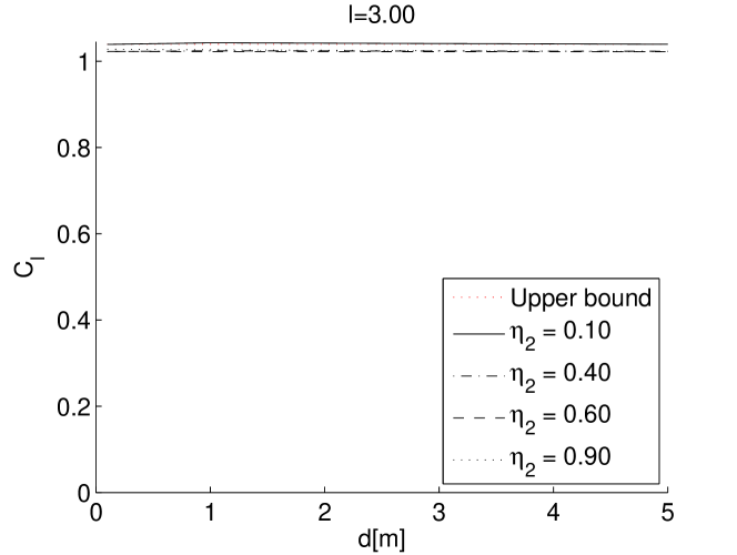
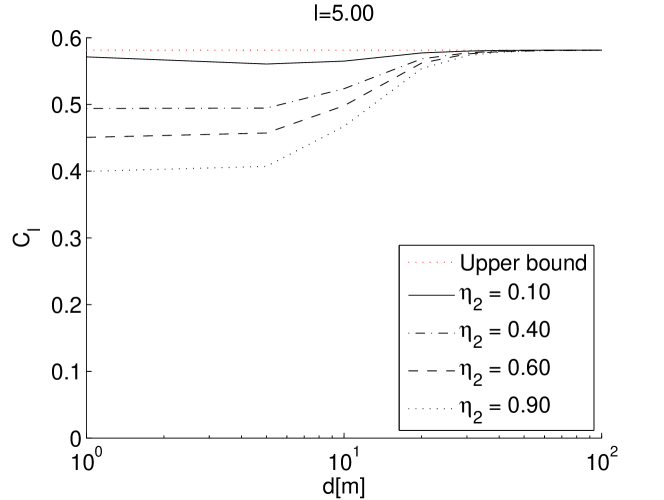
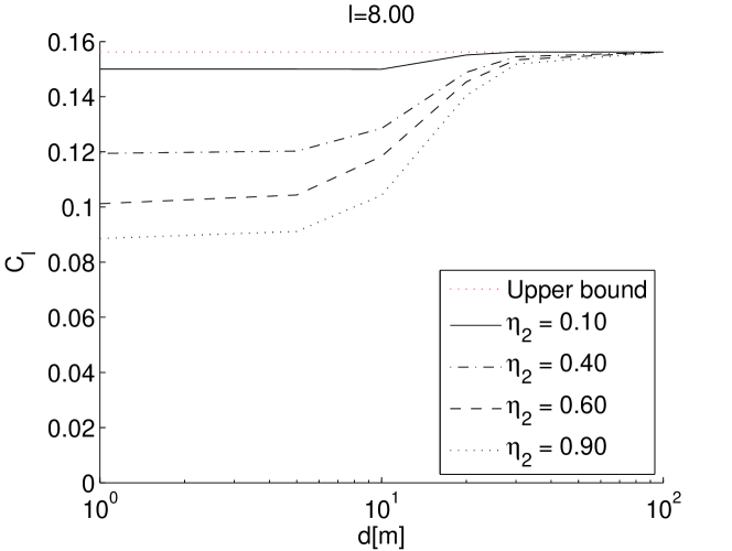
Figure 1: Upper and lower bounds on achievable rates of channels with a single interferer for $l=3$m, $l=5$m, and $l=8$m. The lower bound is given for different values of $\eta_{2}$ (the upper bound is independent of $\eta_{2}$). The upper bound coincides with the lower-bound for $d=100$m.

In order to illustrate our results, we consider a channel with a single interferer ($I=2$). We take $N=80$ which is around the maximum packet size we can use to have reasonable simulation times. We also take $M=5$ corresponding to a 5-tap receiver, which is also aroung the maximum $M$ we can simulate.

For channel statistics we use the measurements from [6] which says that the tap energy drops linearly with the tap delay. Approximately 14% of the total energy is in the first 5 taps. We also assume here that taps are independent.

In this section we are interested in comparing performance of channels for different channel parameters. In order to avoid additional unnecessary variance in our results, we will assume here that ${\bf{h}}_{1}$ is given. Similar results hold for different values of ${\bf{h}}_{1}$ (hence will hold for the average channel realisations as well).

We further suppose that the distance between receiver 1 and receiver 0 is $l$ and the distance between interferer 2 and receiver 1 is $d$. Both 1 and 2 transmit with transmitting power $P_{\mbox{trans}}=0.1$mW. The average received power at distance $l$ is $P_{\mbox{rcv}}(l)=P_{\mbox{trans}}\,b\,l^{-\alpha}$ where $b=10^{-5.5},\alpha=3.3$ are taken from [13]. White-noise power is $\sigma_{W}^{2}=10^{-13}W$. The maximum communication range of such a system is around 10m, so in our simulations we use link sizes of $l=$3,5,8m.

In order to illustrate the result we consider a scenario in which we fix $\eta_{1}=0.5$ and for different $l$ we vary $d$ and $\eta_{2}$. The results are shown in Figure 1. We see that for $l=3$m the achievable rate is insensitive to the interference. For $l=5$m and $l=8$m the rate decreases when the interferer is closer than $d<30$m. However, it drops until $d=5$m, and for smaller $d$ the achievable rate stays constant. This shows us that when the interferer is close enough, MLE decoding actually performs a kind of multi-user detection, successfully extracting the interference and preventing a further drop in performance.

We further compare the achievable rate on a channel with interferer to the achievable rate without interferer (or equivalently sufficiently large $d$, e.g. $d=100$m). We see that even when the interferer is much closer than the transmitter, the rate drop is not significant. In our examples, it is never more than 50%. This is in contrast to [1] where the rate drops to zero if interference is much stronger than the signal itself.

VI Conclusions and Future Work

We analyzed the performance of coherent IR-UWB channel with MLE detector. We presented a novel procedure to calculate a lower-bound on achievable rates using random-coding techniques and Monte-Carlo simulations. Using this bound we are able to show that the performance of an MLE detector is significantly better than the performance of a widely used nearest-neighbor detector in presence of a strong impulsive interference. This suggested that the use of a more complex MLE detector may completely eliminate the need for a medium access protocol in IR-UWB networks. The analysis of more complex networking scenarios and different medium access protocols is left for future work.

In the appendix we explain how to calculate the channel output distribution $P({\bf{R}}={\bf{Y}}\,|\,{\bf{V}},{\bf{h}}_{1})$ and $J({\bf{V}},{\bf{W}},{\bf{h}}_{1})=\int_{\bf{Y}}P({\bf{R}}={\bf{Y}}\,|\,{\bf{V}},{\bf{h}}_{1})P({\bf{R}}={\bf{Y}}\,|\,{\bf{W}},{\bf{h}}_{1})d{\bf{Y}}$. First, conditional to the channel realisation ${\bf{H}}$ and the transmitted symbols ${\bf{U}}$, the channel outputs $R=\{r_{m}[w]\}$ are Gaussian i.i.d. RV with distribution

$$P({\bf{R}}={\bf{Y}}|{\bf{U}},{\bf{H}})=\left({1\over\sqrt{2\pi\sigma_{W}^{2}}}\right)^{MN}\times$$

$$\times \exp\left(-\sum_{w=1}^{N}\sum_{m=1}^{M}(y_{m}[w]-\sum_{i=1}^{I}v_{i}[w]A_{i}h_{im})^{2}/2\sigma_{W}^{2}\right).$$

Also, each channel response ${\bf{h}}_{i}$ is multivariate Gaussian with distribution

$$P({\bf{H}}_{-1})=\left({1\over\sqrt{(2\pi)^{M}|T|}}\right)^{I-1}\exp\left(-{1\over 2}\sum_{i=2}^{I}{\bf{h}}_{i}^{T}T^{-1}{\bf{h}}_{i}\right),$$

Thus, we have

$$P({\bf{R}}={\bf{Y}}\,|\,{\bf{V}},{\bf{h}}_{1})=\mathbb{E}_{{\bf{H}}_{-1}}(P({\bf{R}}={\bf{Y}}|{\bf{V}},{\bf{H}}))=$$

$$= \int_{{\bf{H}}_{-1}}\left({1\over\sqrt{(2\pi)^{M}|T|}}\right)^{I-1}\left({1\over\sqrt{2\pi\sigma_{W}^{2}}}\right)^{MN}\times$$

$$\times \exp\left(-\sum_{i=1}^{I}{{\bf{h}}_{i}^{T}T^{-1}{\bf{h}}_{i}\over 2}\right)\times$$

$$\times \exp\left(-\sum_{w=1}^{N_{1}}\sum_{m=1}^{M}{(y_{m}[w]-\sum_{i=1}^{I}v_{i}[w]A_{i}h_{im})^{2}\over 2\sigma_{W}^{2}}\right)d{\bf{H}}_{-1}$$

which is again a multivariate Gaussian and can be expressed in closed form. Similarly, since $P({\bf{R}}={\bf{Y}}\,|\,{\bf{V}},{\bf{h}}_{1})$ is exponential, $J({\bf{V}},{\bf{W}},{\bf{h}}_{1})$ is also exponential and can be calculated explicitly. However, both expressions are long and we do not give them here.

References

- [1] G. Durisi and S. Benedetto, “Performance evaluation of TH-PPM UWB systems in the presence of multiusers interference,” IEEE Communication Letters, vol. 7, no. 5, May 2003.
- [2] A. Lapidoth, “Nearest neighbor decoding for additive non-gausian noise channels,” IEEE Transactions on Information Theory, vol. 42, no. 5, pp. 1520–1529, September 1996.
- [3] G. Durisi and G. Romano, “On the validity of gaussian approximation to characterize the multiuser capacity of UWB TH-PPM,” in Proc. UWBST, 2002.
- [4] R. Merz and J.-Y. Le Boudec, “Conditional bit error rate for an impulse radio UWB channel with interfering users,” in Proc. ICUWB, 2005.
- [5] Y. Souilmi and R. Knopp, “On the achievable rates of ultra-wideband systems in multipath fading environments,” in ISIT, July 2003.
- [6] Y. Souilmi and K. Raymond, “Challenges in UWB signaling for ad-hoc networking,” in DIMACS Series, November 2003, pp. 271–284.
- [7] X. Luo and G. Giannakis, “Achievable rates of transmitted-reference ultra-wideband radio with PPM,” IEEE Transactions on Communications, vol. 54, no. 9, pp. 1536–1541, September 2006.
- [8] C. Steiner and K. Witrisal, “Multiuser interference modeling and suppression for a multichannel differential IR-UWB system,” in ICUWB, 2005.
- [9] D. Tse and P. Viswanath, Fundamentals of Wireless Communication. Cambridge University Press, 2005.
- [10] I. E. Telatar and D. N. C. Tse, “Capacity and mutual information of wideband multipath fading channels,” IEEE Transactions on Information Theory, vol. 46, no. 4, pp. 1384–1400, July 2000.
- [11] M. Win and R. Scholtz, “Ultra-wide bandwidth time-hopping spread-spectrum impulse radio for wireless multiple-access communications,” IEEE Transactions on Communications, vol. 48, no. 4, pp. 679–691, April 2000.
- [12] J.-Y. Le Boudec, “Performance evaluation,” EPFL,” Lecture Notes, 2006. [Online]. Available: http://ica1www.epfl.ch/perfeval/
- [13] S. Ghassemzadeh and V. Tarokh, “Uwb path loss characterization in residential environments,” in IEEE Radio Frequency Integrated Circuits (RFIC) Symposium, June 2003, pp. 501–504.