Invariant template matching in systems with spatiotemporal coding: a vote for instability

Abstract

We consider the design of a pattern recognition that matches templates to images, both of which are spatially sampled and encoded as temporal sequences. The image is subject to a combination of various perturbations. These include ones that can be modeled as parameterized uncertainties such as image blur, luminance, translation, and rotation as well as unmodeled ones. Biological and neural systems require that these perturbations be processed through a minimal number of channels by simple adaptation mechanisms. We found that the most suitable mathematical framework to meet this requirement is that of weakly attracting sets. This framework provides us with a normative and unifying solution to the pattern recognition problem. We analyze the consequences of its explicit implementation in neural systems. Several properties inherent to the systems designed in accordance with our normative mathematical argument coincide with known empirical facts. This is illustrated in mental rotation, visual search and blur/intensity adaptation. We demonstrate how our results can be applied to a range of practical problems in template matching and pattern recognition.

1 Notational preliminaries

We define an image as a mapping $S_{0}(x,y)$ from a class of locally bounded mappings $\mathcal{S}\subseteq L_{\infty}(\Omega_{x}\times\Omega_{y})$, where $\Omega_{x}\subseteq\mathbb{R}$, $\Omega_{y}\subseteq\mathbb{R}$, and ${L}_{\infty}(\Omega_{x}\times\Omega_{y})$ is the space of all functions $f:\Omega_{x}\times\Omega_{y}\rightarrow\mathbb{R}$ such that $\|f\|_{\infty}={\mathrm{ess}}\sup\{\|f(x,y)\|,x\in\Omega_{x},\ y\in\Omega_{y}\}<\infty$. Symbols $x$, $y$ denote variables on different spatial axes. The value of $S_{0}(x,y)$ depends on the characteristic value of interest (e.g. brightness, contrast, color, etc.). We assume that an image can be described within the system as a set of a-priory specified templates, $S_{i}(x,y)\in\mathcal{S}$, $i\in\mathcal{I}\subset\mathbb{N}$, where $\mathcal{I}$ is the set of indices of all templates associated with the image $S_{0}(x,y)\in\mathcal{S}$. Symbol $\mathcal{I}^{+}$ is reserved for $\mathcal{I}^{+}=\mathcal{I}\cup 0$.

The solution of a system of differential equations $\dot{\mathbf{x}}=\mathbf{f}(\mathbf{x},t,\mbox{\boldmath$\theta$},\mathbf{u}(t))$, $\mathbf{u}:\mathbb{R}_{\geq 0}\rightarrow\mathbb{R}^{m}$, $\mbox{\boldmath$\theta$}\in\mathbb{R}^{d}$ passing through point $\mathbf{x}_{0}$ at $t=t_{0}$ will be denoted for $t\geq t_{0}$ as $\mathbf{x}(t,\mathbf{x}_{0},t_{0},\mbox{\boldmath$\theta$},\mathbf{u})$, or simply as $\mathbf{x}(t)$ if it is clear from the context what the values of $\mathbf{x}_{0},\mbox{\boldmath$\theta$}$ are and how the function $\mathbf{u}(t)$ is defined.

By ${L}^{n}_{\infty}[t_{0},T]$, $t_{0}\geq 0$, $T\geq t_{0}$ we denote the space of all functions $\mathbf{f}:\mathbb{R}_{\geq 0}\rightarrow\mathbb{R}^{n}$ such that $\|\mathbf{f}\|_{\infty,[t_{0},T]}={\mathrm{ess}}\sup\{\|\mathbf{f}(t)\|,t\in[t_{0},T]\}<\infty$; $\|\mathbf{f}\|_{\infty,[t_{0},T]}$ stands for the ${L}^{n}_{\infty}[t_{0},T]$ norm of $\mathbf{f}(t)$.

Let $\mathcal{A}$ be a set in ${\mathbb{R}^{n}}$ and $\|\cdot\|$ be the usual Euclidean norm in $\mathbb{R}^{n}$. By the symbol $\left\|\cdot\right\|_{\mathcal{A}}$ we denote the following induced norm:

$$\left\|\mathbf{x}\right\|_{\mathcal{A}}=\inf_{\mathbf{q}\in\mathcal{A}}\{\|\mathbf{x}-\mathbf{q}\|\}$$

In case $x$ is a scalar and $\Delta\in\mathbb{R}_{>0}$, notation $\|x\|_{\Delta}$ stands for the following

$$\|x\|_{\Delta}=\left\{\begin{array}[]{ll}|x|-\Delta,&|x|>\Delta\\ 0,&|x|\leq\Delta\end{array}\right.$$

2 Introduction

Template matching is the oldest and most common method for detecting an object in an image. According to this method the image is searched for items that match a template. A template consists of one or more local arrays of values representing the object, e.g. intensity, color, or texture. Between these templates and certain domains of the image, a similarity value is calculated, and a domain is associated with a template once their similarity exceeds a given threshold.

Despite the simple and straightforward character of this method, its implementation requires us to consider two fundamental problems. The first relates to what features should be compared between the image $S_{0}(x,y)$ and the template $S_{i}(x,y)$, $i\in\mathcal{I}$. The second problem is how this comparison should be done.

The normative answer to the question of what features should be compared invokes solving the issue of optimal image representation, ensuring most effective utilization of available resources and, at the same time, minimal vulnerability to uncertainties. Principled solutions to this problem are well-known from the literature and can be characterized as spatial sampling. For example, when the resource is frequency bandwidth of a single measurement measurement mechanism, the optimality of spatially sampled representations is proven in Gabor’s seminal work [9]. In classification problems, the advantage of spatially sampled image representations is demonstrated in [42]. In general, these representations are obtained naturally when balancing the system resources and uncertainties in the measured signal. A simple argument supporting this claim is provided in Appendix 1.

The simplest form of spatial sampling can be achieved by factorizing both the domain $\Omega_{x}\times\Omega_{y}$ of the image $S_{0}$ and the templates $S_{i}$, $i\in\mathcal{I}$ into subsets:

$$\Omega_{x}\times\Omega_{y}=\bigcup_{t}\Omega_{x,t}\times\Omega_{y,t},\ t\in\Omega_{t},\ \Omega_{x,t}\subseteq\Omega_{x},\ \Omega_{y,t}\subseteq\Omega_{y}.$$ (1)

Factorization (1) induces sequences $\{S_{i,t}\}$, where $S_{i,t}$ are the restrictions of mappings $S_{i}$ to the domains $\Omega_{x,t}\times\Omega_{y,t}$. These sequences constitute sampled representations of $S_{i}$, $i\in\mathcal{I}^{+}$ (see Figure 1).

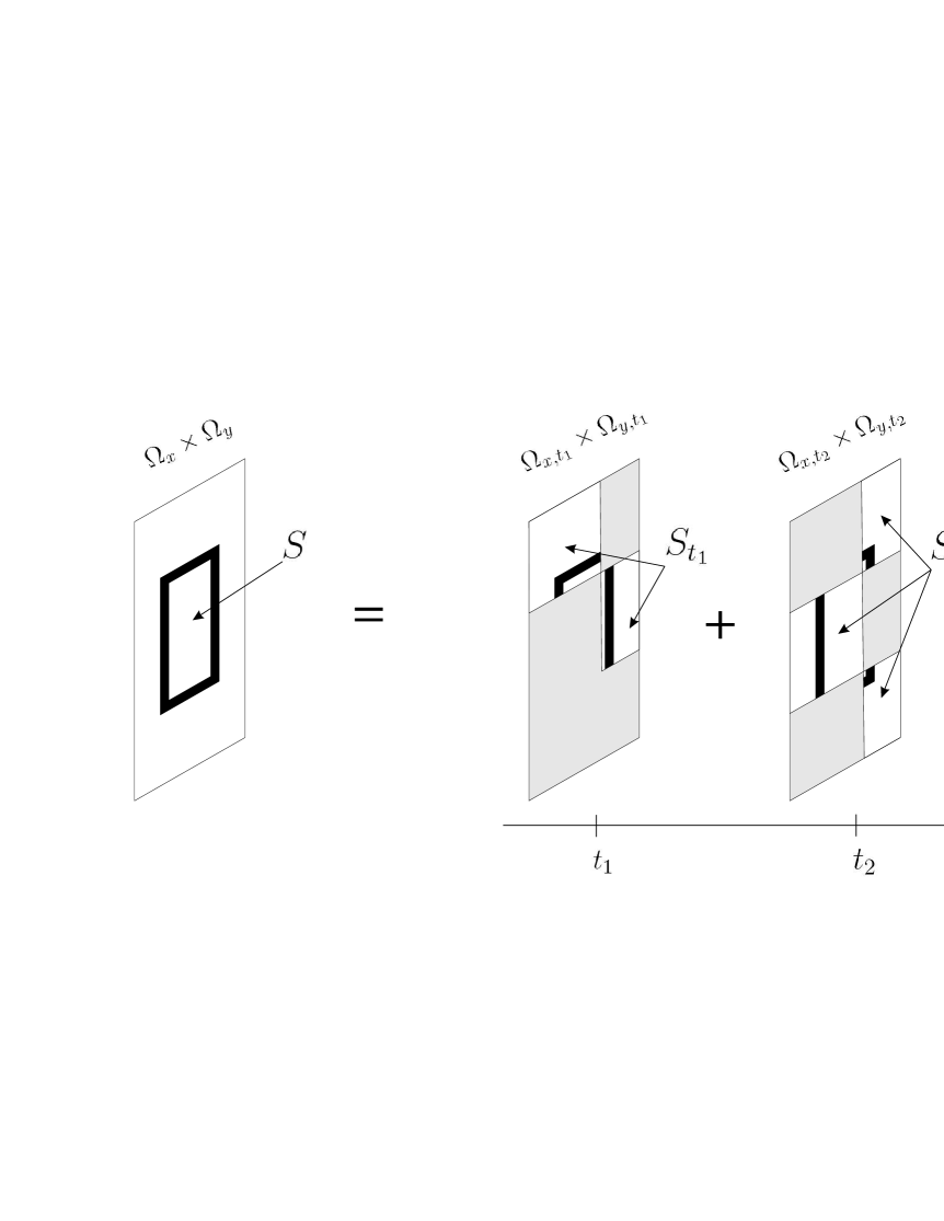
Figure 1: Spatial sampling of image $S(x,y):\Omega_{x}\times\Omega_{y}\rightarrow\mathbb{R}_{+}$ according to the factorization of $\Omega_{x}\times\Omega_{y}$ into subsets $\Omega_{x,t_{1}}\times\Omega_{y,t_{1}}$, $\Omega_{x,t_{2}}\times\Omega_{y,t_{2}}$, $\Omega_{x,t_{3}}\times\Omega_{y,t_{3}}$

Notice that the sampled image and template representations $\{S_{i,t}\}$ are, strictly speaking, sequences of functions. In order to compare them, scalar values $f(S_{i,t})$ are normally assigned to each $S_{i,t}$. Examples include various functional norms, correlation functions, spectral characterizations (average frequency or phase), or simply weighted sums of the values of $S_{i,t}$ over the entire domain $\Omega_{x,t}\times\Omega_{y,t}$. Formally, $f$ could be defined as a functional, which maps restrictions $S_{i,t}$ into the field of real numbers:

$$\begin{split}f:&\ L_{\infty}(\Omega_{x,t}\times\Omega_{y,t})\rightarrow\mathbb{R}\end{split}$$ (2)

This formulation allows a simple representation of images and templates as sequences of scalar values $\{f(S_{i,t})\}$, $i\in\mathcal{I}^{+}$, $t\in\Omega_{t}$. We will therefore adopt this method here.

The answer to the second question, that of how the comparison is done, involves finding the best possible and most simple way to utilize information provided by a given image representation, at the same time ensuring invariance to basic distortions. Despite the fact that considerable attention has been given to this problem, a principled and unified solution is not yet available. The primary goal of our current contribution is to present a unified framework to solve this problem for a class of systems of sufficiently broad theoretical and practical relevance.

We consider the class of systems in which spatially sampled image representations are encoded as temporal sequences. In other words, parameter $t$ in the notation $f(S_{i,t})$ is the time variable. This type of representation is frequently encountered in neuronal networks [13] (see also references therein), and so such systems have a claim to biological plausibility. In addition, they enable a simple solution to a well-known dilemma. The dilemma is about whether comparison between templates and image domains should be made on a large, global, or on a small, local scale. The solution to this dilemma consists in temporal integration. Let, for instance, $\Omega_{t}=[0,T]$, $T\in\mathbb{R}_{>0}$. Then an example of a temporally-integral, yet spatially sampled, representation is:

$$f(S_{i,t})\mapsto\phi_{i}(t)=\int_{0}^{t}f(S_{i,\tau})d\tau,\ t\in[0,T],\ i\in\mathcal{I}^{+}$$ (3)

The temporal integral $\phi_{i}(t)$ contains both spatially local and global image characterizations. Whereas its time-derivative at $t$ equals to $f(S_{i,t})$ and corresponds to spatially sampled, local representation $S_{i,t}$, the global representation $\phi_{i}(T)$ equals to the integral, cumulative characterization of $S_{i}$. An example illustrating these properties is provided in Figure 2.

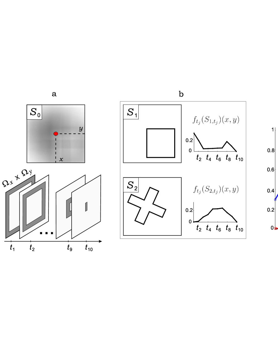
Figure 2: Spatiotemporal image representation via spatial sampling and temporal integration. Panel $a$ contains original object, $S_{0}$; $(x,y)$ marks a point on the image with respect to which the correlation is calculated; factorization of the domain $\Omega_{x}\times\Omega_{y}$ into ten nonintersecting subsets $\Omega_{x}\times\Omega_{y}=\cup_{j=1}^{10}\Omega_{x,t_{j}}\times\Omega_{y,t_{j}}$. Panel $b$ – templates $S_{1}$, $S_{2}$ and plots of $f_{t_{j}}(S_{1,t_{j}})(x,y)$, $f_{t_{j}}(S_{2,t_{j}})(x,y)$ – the values of the normalized correlation between $S_{i,t_{j}}=S_{i}(\Omega_{x,t_{j}}\times\Omega_{y,t_{j}})$ and $S_{0}(\Omega_{x,t_{j}}\times\Omega_{y,t_{j}})$. Panel $c$ – plots of the values of (3) as a function of parameter $t$ for templates $S_{1}$ (blue line) and $S_{2}$ (red line).

A further advantage of spatiotemporal representations $\phi_{i}(t)$ is that they offer powerful mechanisms for comparison, processing and matching of $\phi_{i}(t)$, $i\in\mathcal{I}$. These mechanisms can generally be characterized in terms of dynamic oscillator networks which synchronize when their inputs are converging to the same function.

Despite advantages such as optimality, simplicity and biological plausibility, there are theoretical issues which have prevented wide application of spatiotemporal representations to template matching. The most important issues, from the authors’ viewpoint, are, first, how to achieve effective recognition in the presence of modeled disturbances, of which the most common ones are blur, luminance, and rotational and translational distortion. Second, how to take into account inevitable unmodeled perturbations.

The first class of problems amounts to finding an identification/adaptation algorithm capable of reconstructing parameters of generally nonlinear perturbations. Currently available approaches either are restricted to linear parametrization of disturbances, involve overparametrization, or use domination feedback. However, linear parametrization is too restricted to be plausible, overparametrization is expensive in terms of the number of adjustable units, and domination lacks adequate sensitivity. For these reasons these methods remain unsatisfactory. The second class of problems calls for procedures for recognizing an image from its perturbed temporal representation $\phi_{i}(t)$. At this level the system is facing contradictory requirements of ensuring robust performance while being highly sensitive to minor changes in the stimulation.

Both these problems are traditionally dealt with within the concept of Lyapunov-stable attractors. By allowing the system to converge on an attractor, it is possible to eliminate modeled and unmodeled distortions and thus, for instance, complete an incomplete pattern in the input [1, 8, 16, 19, 32]. The advantage of these methods resides in the robustness inherent in uniform asymptotic Lyapunov stability. This advantage, however, comes at a cost: such systems are generally lacking in flexibility. Each stable attractor represents one pattern; but often an image contains more than one pattern. When the system is steered to one template, the other is lost from the representation. It would, therefore, be preferable to have a system that allows flexible switching between alternative patterns. Yet, the very notion of stable convergence to an attractor prevents switching and exploration across patterns. Furthermore, as we will show, for a class of the images with multiple representations and various symmetries globally stable solutions to the problem of invariant template matching may not even exist.

We propose a unifying framework capable of combining robustness and flexibility. In contrast to common intuitions, which aim at achieving desired robustness by means of stable attractors, we advocate instability as an advantageous substitute. We demonstrate that a specific type of instability, the concept of weakly attracting sets, provides both the necessary invariance and flexibility.

To illustrate these principles we designed a recognition system consisting of two major subcomponents (see Figure 3).

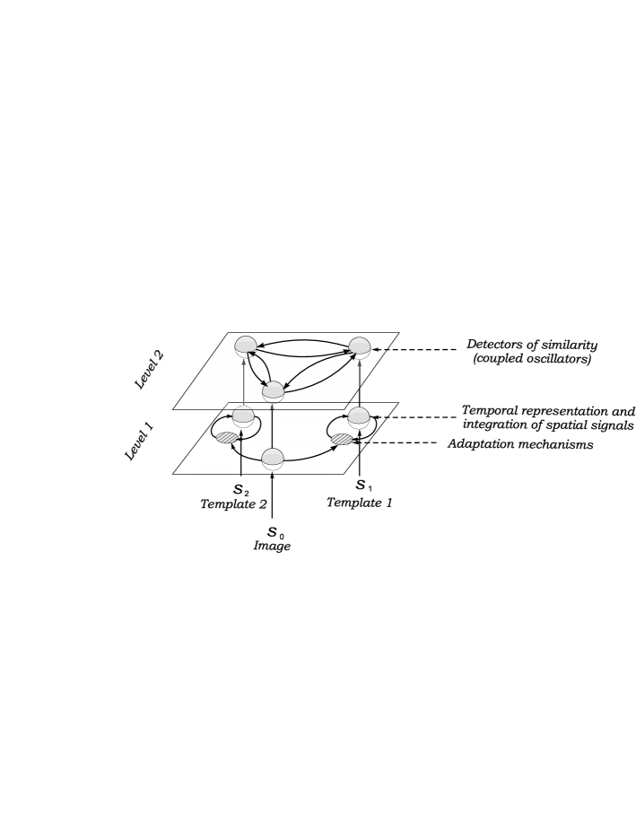
Figure 3: General scheme of a system for adaptive template matching using temporal codes. Level $1$ contains the adaptive compartments. Its functional role is to ensure invariance to modeled uncertainties. Level $2$ corresponds to the comparison compartments and consists of coupled nonlinear oscillators. Solid arrows represent the information flow in the system.

The first is an adaptive component in which information is processed by a class of spatiotemporal filters. These filters represent internal models of distortions. The models of most common distortions, including rotation, translation, and blur, are often nonlinearly parameterized. Until recently adequate compensatory mechanisms for nonlinear parameterized uncertainties where unexplored territory. In recent work [41] we have shown that the problem of non-dominating adaptation could, in principle, be solved within the concept of Milnor or weak, unstable attractors. Here we provide a solution to this problem that will enable systems to deal with specific nonlinearly parameterized models of distortions that are typical for a variety of optical and geometrical perturbations.

The second component consists of a network of coupled nonlinear oscillators. These operate as coincidence detectors. Each oscillator in our system represents a Hindmarsh-Rose model neuron. These model neurons are generally believed to provide a good qualitative approximation to biological neuron behavior. At the same time they are computationally effective in simulations [20]. For networks of these oscillators we prove, first of all, boundedness of the state of the perturbed solutions. In addition, we specify the parameter values which lead to emergence of globally stable invariant manifolds in the system state space. Although we do not provide explicit criteria for meta-stability in this class of networks, the conditions presented allow us to narrow substantially the domain of relevant parameter values in which this behavior is to be found.

There is an interesting consequence to the unstable character of the compensation for modeled perturbations. When the system negotiates multiple classes of uncertainties simultaneously (e.g. focal/contrast and intensity/luminance), different types of compensatory adjustments occur at different time scales. Adaptation at different time scales is a well-known phenomenon in biological visual systems, in particular when light/dark adaptation is combined with optical/neuronal blur [18, 27, 29, 33]; experiments have shown that combined adaptation processes take place simultaneously but at different time-scales [3, 5, 34, 35]. Our analytical study suggests that this difference in time-scales emerges naturally as a sufficient condition for the proper operation of our system.

This paper is organized as follows. In Section 3 we provide a formal description of the class of images and templates, and formally state the problems of our study. In Section 4 we provide the main results of our present contribution. In Section 5 we discuss the theoretical results, relate them to relevant observations in the empirical literature on visual perception and adaptation, and provide an application of our approach to a realistic pattern recognition problem: the detection of morphological changes in dendritic spines based on measurements obtained from multiphoton scanning microscope.

3 Preliminaries and problem formulation

We assume that the values $S_{0}(x,y)$ of the original image are not available explicitly to the system; the system is able to measure only perturbed values of $S_{0}(x,y)$. Perturbation is defined as a mapping $\mathcal{F}$:

$$\mathcal{F}[S_{0},\mbox{\boldmath$\theta$}]:\ L_{\infty}(\Omega_{x}\times\Omega_{y})\times\mathbb{R}^{d}\rightarrow L_{\infty}(\Omega_{x}\times\Omega_{y}),$$

where $\theta$ is the vector of parameters of the perturbation. The values of $\theta$ are assumed to be unknown a-priori, whereas the mapping $\mathcal{F}$ is known.

In systems for processing spatial information, mappings $\mathcal{F}$ often belong to a specific class that can be defined as follows:

$$\begin{split}\mathcal{F}[S_{0},\mbox{\boldmath$\theta$}]&=\theta_{1}\cdot\bar{\mathcal{F}}[S_{0},\theta_{2}],\ \theta_{1}\in\mathbb{R},\ \theta_{2}\in\mathbb{R}\\ \bar{\mathcal{F}}[S_{0},\theta_{2}]:&\ L_{\infty}(\Omega_{x}\times\Omega_{y})\times\mathbb{R}\rightarrow L_{\infty}(\Omega_{x}\times\Omega_{y}),\\ \mbox{\boldmath$\theta$}&=(\theta_{1},\theta_{2})\end{split}$$ (4)

Parameter $\theta_{1}\in[\theta_{1,\min},\theta_{1,\max}]\subset\mathbb{R}$ in (4) models linear perturbations, for instance variations of overall brightness or intensity of the original image $S_{0}$. It can be interpreted also as an a-priori unknown gain in the measurement channel of a sensor. Mapping $\bar{\mathcal{F}}(S_{0},\theta_{2})$ in (4), parameterized by $\theta_{2}\in[\theta_{2,\min},\theta_{2,\max}]\subset\mathbb{R}$, corresponds to typical nonlinear perturbations of image $S_{0}$. Table 1 provides examples of these perturbations, their mathematical models and the physical meaning of parameter $\theta_{2}$.

Table 1: Examples of typical nonlinear perturbations of $S_{0}$. Parameter $\Delta_{\theta}$ in the right column is a positive constant

Physical meaning	Mathematical model	Domain of
	of $\bar{\mathcal{F}}[S_{0},\theta_{2}]$	physical relevance
Translation (in $x$ dimension)	$\bar{\mathcal{F}}[S_{0},\theta_{2}]=S_{0}(x+\theta_{2},y)$	$-\Delta_{\theta}\leq\theta_{2}\leq\Delta_{\theta}$
$\theta_{2}$ – shift
Scaling (in $x$ dimension)	$\bar{\mathcal{F}}[S_{0},\theta_{2}]=S_{0}(\theta_{2}\cdot x,y)$	$0<\theta_{2}\leq\Delta_{\theta}$
$\theta_{2}$ – scaling factor
Rotation	$\bar{\mathcal{F}}[S_{0},\theta_{2}]=S_{0}(x_{r}(x,y,\theta_{2}),y_{r}(x,y,\theta_{2}))$	$0\leq\theta_{2}\leq 2\pi$
around the origin
	$x_{r}(x,y,\theta_{2})=\cos(\theta_{2})x-\sin(\theta_{2})y$
$\theta_{2}$ – angle of rotation	$y_{r}(x,y,\theta_{2})=\sin(\theta_{2})x+\cos(\theta_{2})y$
Image blur [4]	$\bar{\mathcal{F}}[S_{0},\theta_{2}]=\int_{\Omega_{x}\times\Omega_{y}}h\cdot S_{2}(\xi,\gamma)d\xi d\gamma$	$0<\theta_{2}\leq\Delta_{\theta}$
(not normalized)
$\theta_{2}$ – blur parameter	1) Gaussian: $$h=\exp^{-\frac{1}{\theta_{2}}((x-\xi)^{2}+(y-\gamma)^{2})}$$
	2) Out-of-focus: $$h=\left\{\begin{array}[]{ll}\frac{1}{\pi\theta_{2}^{2}},&\sqrt{(x-\xi)^{2}+(y-\gamma)^{2}}\leq\theta_{2}\\ 0,&\mathrm{else}\end{array}\right.$$

Throughout the paper we assume that mappings $\bar{\mathcal{F}}[S_{0},\theta_{2}]$ are Lipschitz in $\theta_{2}$:

$$\begin{split}\exists\ D\in\mathbb{R}_{>0}:\ \ \left|\bar{\mathcal{F}}[S_{0},\theta_{2}^{\prime}](x,y)-\bar{\mathcal{F}}[S_{0},\theta_{2}^{\prime\prime}](x,y)\right|&\leq D|\theta_{2}^{\prime}-\theta_{2}^{\prime\prime}|,\\ \forall\ (x,y)\in\Omega_{x}\times\Omega_{y},&\ \theta_{2}^{\prime},\theta_{2}^{\prime\prime}\in\mathbb{R}\end{split}$$ (5)

Notice that, strictly speaking, several typical transformations such as translation, scaling, and rotation, are not always Lipschitz. This is because image $S_{0}$ can, for instance, have sharp edges which corresponds to discontinuities in $x,y$. In practice, however, prior application of a blurring linear filter will render sharp edges in an image smooth, thus assuring that condition (5) applies.

The image $\mathcal{F}[S_{0},\mbox{\boldmath$\theta$}]$ is assumed to be spatially sampled according to factorization (1):

$$\mathcal{F}_{t}[S_{0},\mbox{\boldmath$\theta$}](x,y)=\left\{\begin{array}[]{ll}\mathcal{F}[S_{0},\mbox{\boldmath$\theta$}](x,y),&(x,y)\in\Omega_{x,t}\times\Omega_{y,t},\\ 0,&\mathrm{else}\end{array}\right.\ \ t\in\Omega_{t}$$ (6)

Because index $t$ in (6) is assumed to be a time variable we let $\Omega_{t}=[0,\infty)$. To each $\mathcal{F}_{t}[S_{0},\mbox{\boldmath$\theta$}]$ a value $f(\mathcal{F}_{t}[S_{0},\mbox{\boldmath$\theta$}])\in\mathbb{R}$ is assigned. Formally this procedure can be defined by a functional which maps mappings $\mathcal{F}_{t}[S_{0},\mbox{\boldmath$\theta$}]$ into the real values:

$$f:L_{\infty}(\Omega_{x}\times\Omega_{y})\rightarrow\mathbb{R}.$$ (7)

In the singular case, when $\Omega_{x,t}\times\Omega_{y,t}$ is a point $(x_{t},y_{t})$, the mapping $\mathcal{F}_{t}[S_{0},\mbox{\boldmath$\theta$}](x,y)$ and functional $f$ will be defined as $f=\mathcal{F}_{t}[S_{0},\mbox{\boldmath$\theta$}](x_{t},y_{t})=\mathcal{F}[S_{0},\mbox{\boldmath$\theta$}](x_{t},y_{t})$.

We concentrated our efforts on obtaining a principled solution to the problem of invariant template matching in systems with spatiotemporal processing of information. For this reason we prefer not to provide a specific description of functionals $f$. We do, however, restrict our consideration to linear and Lipschitz functionals, e.g. the functionals satisfying the following constraints:

$$f(\kappa\mathcal{F})=\kappa f(\mathcal{F}),\ \forall\ \kappa\in\mathbb{R},\ \ \left|f(\mathcal{F})-f(\mathcal{F}^{\prime})\right|\leq D_{2}\|\mathcal{F}-\mathcal{F}^{\prime}\|_{\infty},\ \ D_{2}\in\mathbb{R}_{>0}$$ (8)

Examples of functionals $f$ satisfying conditions (8) and their physical interpretations are provided in Table 2.

Table 2: Examples of spatially-sampled representations of $S_{0}$

Physical meaning	Mathematical model of $f$
Spectral power within
the given frequency bands:	$f=\int_{\omega_{a}}^{\omega_{b}}\int_{\omega_{c}}^{\omega_{d}}\left\|\int_{\Omega_{x}\times\Omega_{y}}\mathcal{F}_{t}[S_{0},\mbox{\boldmath$\theta$}](x,y)e^{-j(\omega_{x}x+\omega_{y}y)}dxdy\right\|d\omega_{x}d\omega_{y}$
$\omega_{x}\in[\omega_{a},\omega_{b}]$, $\omega_{y}\in[\omega_{c},\omega_{d}]$
Weighted sum	$f=\int_{\Omega_{x}\times\Omega_{y}}\mathcal{F}_{t}[S_{0},\mbox{\boldmath$\theta$}](x,y)e^{-|x-x_{0}|-|y-y_{0}|}dxdy$
(for instance, convolution
with exponential kernel)	$(x_{0},y_{0})$ is the reference, “attention” point
Scanning the image	$\Omega_{x,t}\times\Omega_{y,t}=(\xi(t),\gamma(t))$
along a given trajectory
$(x(t),y(t))=(\xi(t),\gamma(t))$	$f=\mathcal{F}[S_{0},\mbox{\boldmath$\theta$}](\xi(t),\gamma(t))$

Taking into account (4), (6) and the fact that $f$ is linear, the following equality holds

$$f(\mathcal{F}_{t}[S_{0},\mbox{\boldmath$\theta$}])=\theta_{1}f(\bar{\mathcal{F}}_{t}[S_{0},\theta_{2}]),\ \ \bar{\mathcal{F}}_{t}[S_{0},\theta_{2}]=\left\{\begin{array}[]{ll}\bar{\mathcal{F}}[S_{0},\theta_{2}](x,y),&(x,y)\in\Omega_{x,t}\times\Omega_{y,t},\\ 0,&\mathrm{else}\end{array}\right.$$ (9)

For the sake of compactness, in what follows we replace $f(\bar{\mathcal{F}}_{t}[S_{0},\theta_{2}])$ in the definition of $f(\mathcal{F}_{t}[S_{0},\mbox{\boldmath$\theta$}])$ in (9) with the following notation

$$f(\bar{\mathcal{F}}_{t}[S_{0},\theta_{2}])=f_{0}(t,\theta_{2}),\ f_{0}:\Omega_{t}\times\mathbb{R}\rightarrow\mathbb{R}$$ (10)

Notation $f_{0}(t,\theta_{2})$ in (10) allows us to emphasize the dependence of $f$ on unknown $\theta_{2}$, time variable $t$, and original image $S_{0}$. Subscript “$0$” in (10) indicates that $f_{0}(t,\theta_{2})$ corresponds to the sampled and perturbed $S_{0}$ (equations (4), (7), (8)), and argument $\theta_{2}$ is the nonlinear parameter of the perturbation applied to the image. Adhering to this logic, we introduce the notation

$$f(\mathcal{F}_{t}[S_{i},\mbox{\boldmath$\theta$}])=\theta_{1}f(\bar{\mathcal{F}}_{t}[S_{i},\theta_{2}])=\theta_{1}f_{i}(t,\theta_{2}),$$

where subscript “$i$” indicates that $f_{i}(t,\theta_{2})$ corresponds to the perturbed and sampled template $S_{i}$, and $\theta_{2}$ is the nonlinear parameter of the perturbation applied to the template.

Let us now specify the class of schemes realizing temporal integration of spatially sampled image representations. Explicit realization of temporal integration (3) is not optimal because it might lead to unbounded outputs for a wide class of relevant signals, for instance signals that are constant or periodic with a nonzero average. The behavior of a temporal integrator (3), however, can be fairly well approximated by a first-order linear filter. For the sampled image and template representations $\theta_{1}f_{i}(t,\theta_{2})$, these filters can be defined as follows:

$$\begin{split}\dot{\phi}_{0}&=-\frac{1}{\tau}\phi_{0}+k\cdot\theta_{1}f_{0}(t,\theta_{2})\\ \dot{\phi}_{i}&=-\frac{1}{\tau}\phi_{i}+k\cdot\theta_{1}f_{i}(t,\theta_{2}),\ k,\tau\in\mathbb{R}_{>0},\ i\in\mathcal{I}\end{split}$$ (11)

In contrast to (3), for filters (11) it is ensured that their state remains bounded for bounded inputs. In addition, on a first approximation, equations (11) present a simple model of neural sensors, collecting and encoding spatially-distributed information in the form of a function of time. With respect to the physical realizability of (11), in addition to requirements (5), (8) we shall only assume that spatially sampled representations $\theta_{1}f_{i}(t,\theta_{2})$, $i\in\mathcal{I}^{+}$ of $S_{i}$ ensure the existence of solutions for system (11).

Consider the dynamics of variables $\phi_{0}(t)$ and $\phi_{i}(t)$, $i\in\mathcal{I}$ defined by (11). We say that the $i$-th template matches the image iff for some given $\varepsilon\in\mathbb{R}_{\geq 0}$ the following condition holds

$$\limsup_{t\rightarrow\infty}|\phi_{0}(t)-\phi_{i}(t)|\leq\varepsilon.$$ (12)

The problem, however, is that parameters $\theta_{1}$, $\theta_{2}$ in (11) are unknown a-priori. While perturbations affect the image directly, they do not necessarily influence the templates. Rather to the contrary, for consistent recognition the templates are better kept isolated from external perturbations – at least within the time frame of pattern recognition, although they may, in principle, be affected by adaptive learning on a larger time scale. Having fixed, unmodified templates in comparison with perturbed image representations implies that even in the cases when objects corresponding to the templates are present in the image, temporal image representation $\phi_{0}(t)$ will likely be different from any of the templates, $\phi_{i}(t)$. This will render the chances that condition (12) is satisfied very small, so a template would almost never be detected in an image.

We propose that the proper way for the system to meet requirement (12) is to mimic the effect of disturbances in the template. In order to achieve this template matching system should be able to track the unknown values of parameters ${\theta}_{1}$, $\theta_{2}$. Hence the original equations for temporal integration (11) will be replaced with the following

$$\begin{split}\dot{\phi}_{0}&=-\frac{1}{\tau}\phi_{0}+k\cdot\theta_{1}f_{0}(t,\theta_{2})\\ \dot{\phi}_{i}&=-\frac{1}{\tau}\phi_{i}+k\cdot\hat{\theta}_{i,1}f_{i}(t,\hat{\theta}_{i,2}),\ k,\tau\in\mathbb{R}_{>0},\ i\in\mathcal{I}\end{split}$$ (13)

where $\hat{\theta}_{i,1}$, $\hat{\theta}_{i,2}$ are the estimates of $\theta_{1}$, $\theta_{2}$. The estimates $\hat{\theta}_{i,1}$, $\hat{\theta}_{i,2}$ must track instantaneous changes of ${\theta}_{1}$, $\theta_{2}$. The information required for such an estimation should be kept at the minimal possible level. An acceptable solution would be a simple mechanism capable of tracking the perturbations from the measurements of the image alone. The formal statement of this problem is provided below:

Problem 1 (Invariance)

For a given image $S_{0}$, template $S_{i}$, and their spatiotemporal representations satisfying (5), (8), and (13), find estimates

$$\hat{\theta}_{i,1}=\hat{\theta}_{i,1}(t,\tau,\kappa,\phi_{0},\phi_{i}),\ \ \hat{\theta}_{i,2}=\hat{\theta}_{i,2}(t,\tau,\kappa,\phi_{0},\phi_{i})$$ (14)

as functions of time $t$, variables $\phi_{0}$, $\phi_{i}$ and parameters $\tau$, $\kappa$ such that for all possible values of parameters $\theta_{1}\in[\theta_{1,\min},\theta_{1,\max}]$, $\theta_{2}\in[\theta_{2,\min},\theta_{2,\max}]$

1) solutions of system (13) are bounded;

2) in case $f_{0}=f_{i}$ property (12) is ensured, and

3) the following holds for some $\theta_{1}^{\prime}\in[\theta_{1,\min},\theta_{1,\max}]$, $\theta_{2}^{\prime}\in[\theta_{2,\min},\theta_{2,\max}]$:

$$\begin{split}&\limsup_{t\rightarrow\infty}|\hat{\theta}_{i,1}(t,\tau,\kappa,\phi_{0}(t),\phi_{i}(t))-\theta_{i,1}^{\prime}|\leq\varepsilon_{\theta,1},\ \varepsilon_{\theta,1}\in\mathbb{R}_{+}\\ &\limsup_{t\rightarrow\infty}|\hat{\theta}_{i,2}(t,\tau,\kappa,\phi_{0}(t),\phi_{i}(t))-\theta_{i,2}^{\prime}|\leq\varepsilon_{\theta,2},\ \varepsilon_{\theta,2}\in\mathbb{R}_{+}\end{split}$$ (15)

Once the solution to Problem 1 is found, the next step will be to ensure that similarities (12) are registered in the system. Following the spirit of neural systems and in agreement with the structure in Figure 3, we propose that detection of similarities is realized by a system of coupled oscillators. In particular, we require that states of oscillators $i$ and $0$ converge as soon as the signals $\phi_{0}(t)$, $\phi_{i}(t)$ become sufficiently close.

In the present article we restrict ourselves to the class of systems composed of linearly coupled Hindmarsh-Rose model neurons [17]. This choice is motivated by the fact that these oscillators can reproduce a broad class of behaviors observed in real neurons while being computationally efficient [20]. A network of these neural oscillators can be mathematically described as follows:

$$\mathcal{S}_{D_{i}}:\ \left\{\begin{array}[]{ll}\dot{x}_{i}&=-a{x}_{i}^{3}+b{x}_{i}^{2}+y_{i}-z_{i}+I+u_{i}+\phi_{i}(t),\\ \dot{y}_{i}&=c-d{x}_{i}^{2}-y_{i},\\ \dot{z}_{i}&=\varepsilon(s(x_{i}+x_{0})-z_{i}),\end{array}\right.\ i\in\mathcal{I}^{+}$$ (16)

Variables $x_{i}$, $y_{i}$, $z_{i}$ correspond to membrane potential, and aggregated fast and slow adaptation currents, respectively. Coupling $u_{i}$ in (16) is assumed to be linear and symmetric:

$$\mathbf{u}=\left(\begin{array}[]{c}u_{0}\\ u_{1}\\ \vdots\\ u_{n}\end{array}\right)=\Gamma\left(\begin{array}[]{c}x_{0}\\ x_{1}\\ \vdots\\ x_{n}\end{array}\right),\ \Gamma=\gamma\left(\begin{array}[]{cccc}-n&1&\cdots&1\\ 1&-n&\cdots&1\\ \cdots&\cdots&\cdots&\cdots\\ 1&1&\cdots&-n\\ \end{array}\right),$$ (17)

and parameter $\gamma\in\mathbb{R}_{+}$. Our choice of the coupling function in (17) is motivated by the following considerations. Fist, we wish to preserve the intrinsic dynamics of the neural oscillators when they synchronize, e.g. when $x_{i}=x_{j}$, $y_{i}=y_{j}$, $z_{i}=z_{j}$, $i,j\in\{0,\dots,n\}$. For this reason it is desirable that the coupling vanishes when the synchronous state is reached. Second, we seek for a system in which synchronization between two arbitrary nodes, say the $i$-th and the $j$-th nodes, is determined exclusively by the degree of (mis)matches in $\phi_{i}(t)$, $\phi_{j}(t)$, independently of the activity of other units in the system. Third, the coupling should “pull” the system trajectories towards the synchronous state. Coupling function (17) satisfies all these requirements.

We set parameters of equations (16) to the following values:

$$\begin{array}[]{cccc}a=1,&b=3,&c=1,&d=5,\\ s=4,&x_{0}=1.6,&\varepsilon=0.001,&\end{array}$$ (18)

which correspond to the regime of chaotic bursting in each uncoupled element in (16) [14].

The problem of detection of similarities in $\phi_{0}(t)$ and $\phi_{i}(t)$ can now be stated as follows.

Problem 2 (Detection)

Let system (16), (17) be given and there exist $i\in\mathcal{I}$ such that condition (12) is satisfied. Determine the coupling parameter $\gamma$ as a function of system (16) parameters such that

1) solutions of the system are bounded for all bounded $\phi_{i}$, $i\in\mathcal{I}$;

2) states $(x_{0}(t),y_{0}(t),z_{0}(t))$ and $(x_{i}(t),y_{i}(t),z_{i}(t))$ asymptotically converge to a vicinity of the synchronization manifold $x_{0}=x_{i}$, $y_{0}=y_{i}$, $z_{0}=z_{i}$. In particular,

$$\begin{split}&\limsup_{t\rightarrow\infty}|x_{0}(t)-x_{i}(t)|\leq\delta(\varepsilon)\\ &\limsup_{t\rightarrow\infty}|y_{0}(t)-y_{i}(t)|\leq\delta(\varepsilon)\\ &\limsup_{t\rightarrow\infty}|z_{0}(t)-z_{i}(t)|\leq\delta(\varepsilon),\end{split}$$

where $\delta(\cdot)$ is a non-decreasing function vanishing at zero.

In the next section we present solutions to the problems of invariance and detection. We start from considerations of what would be the most adequate concept of analysis. Our considerations will lead us to conclusion that for solving the problem of invariance, using the concept of Milnor attractors is advantageous over traditional concepts resting on the notion of Lyapunov stability. This implies that the sets to which the estimates $\hat{\theta}_{i,1}$, $\hat{\theta}_{i,2}$ converge should be weakly attracting rather than Lyapunov stable. We present a simple mechanism realizing this requirement for a wide class of models of disturbances. With respect to the second problem, the problem of detection, we provide sufficient conditions for asymptotic synchrony in system (16).

4 Main Results

Consider a system of temporal integrators, (13), in which the template subsystem (second equation in (13)) is designed to mimic the temporal code of an image using adjustment mechanisms (14). Ideally, the template subsystem should have a single adjustment mechanism, which is structurally simple and yet capable of handling a broad class of perturbations. In addition it should require the least possible amount of a-priori information about images and templates.

To search for a possible adaptation mechanism let us first explore the available theoretical concepts which can be used in its derivation. The problem of invariance, as stated in Problem 1, can generally be understood as a specific optimization task. Particular solutions to such tasks as well as choice of the appropriate mathematical tools depend significantly on the following characteristics: uniqueness of the solutions, convexity with respect to parameters, and sensitivity to the input data (images and templates). Let us consider wether the invariant template matching problem meets these requirements.

Uniqueness. Solutions to the problem of invariant template matching are generally not unique. The image may contain multiple instances of the template. Even if there is only a single unique object the template may fit it in multiple ways, for instance because it has rotational symmetry. Both cases are illustrated in Figure 4.

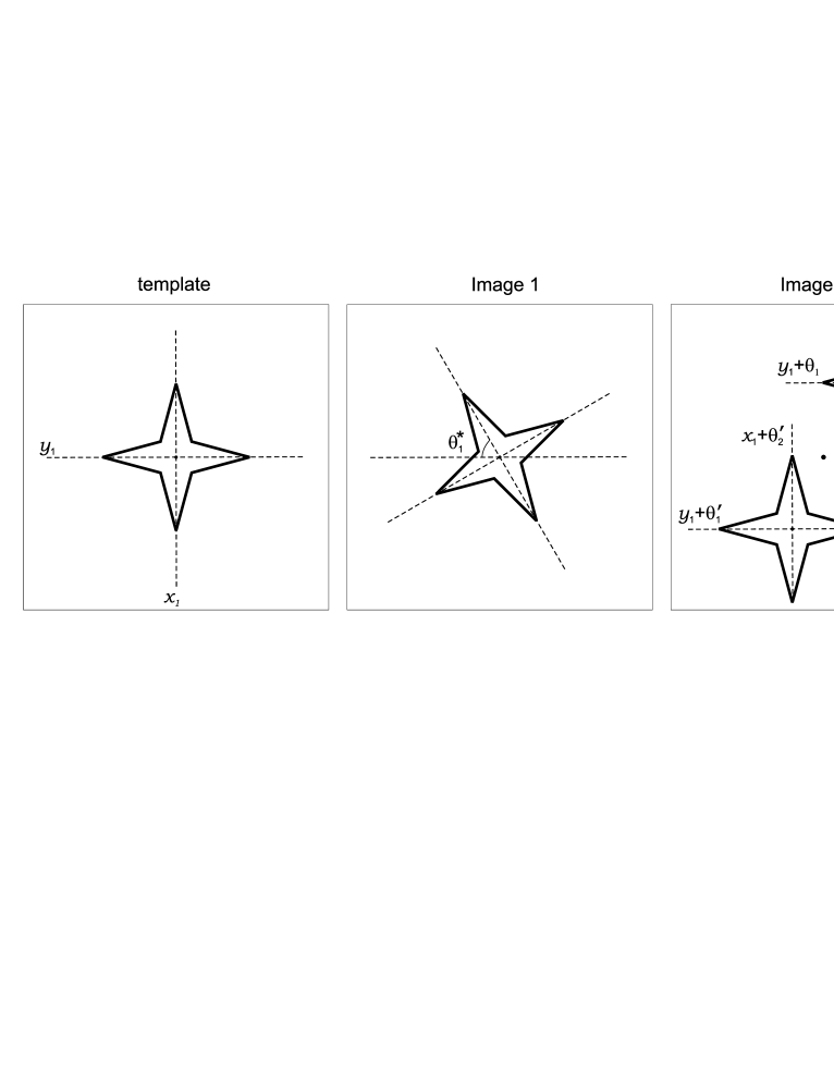
Figure 4: Example of a template and images which lead to non-unique solutions in the problem of invariant template matching. Image 1 is a rotated version of the template. Because the template has rotational symmetry, the angles $\theta_{2}=\theta_{2}^{\ast}\pm\frac{\pi}{2}n$, $n=0,1,\dots$ at which the template and the image match to each other are not unique. Image 2 contains two multiple instances of the template, which also leads to non-uniqueness.

A similar argument applies to translational invariance in the images with multiple instances of the template (right picture in Figure 4).

Non-linearity and non-convexity. The problem of invariant template matching is generally nonlinear and nonconvex in $\theta_{1}$, $\theta_{2}$. The nonlinearity is already evident from Table 1. To illustrate the potential non-convexity consider, for instance, the following function

$$\theta_{1}f_{i}(t,\theta_{2})=\theta_{1}\int_{\Omega_{x,t}\times\Omega_{y,t}}e^{-|x-x_{0}|-|y-y_{0}|}\left(\int_{\Omega_{x}\times\Omega_{y}}e^{-\frac{1}{\theta_{2}}((x-\xi)^{2}+(y-\gamma)^{2}}S_{i}(\xi,\gamma)d\xi d\gamma\right)dxdy$$ (19)

which is a composition of the Gaussian blur model (the forth row in Table 1) with spatial sampling and subsequent exponential weighting (the second row in Table 2). In the literature on adaptation two versions of the convexity requirement are available. The first version applies to the case where the difference $\theta_{1}f_{i}(t,\theta_{2})-\hat{\theta}_{1,i}f_{i}(t,\hat{\theta}_{i,2})$ is not accessible for explicit measurement, and the variables $\phi_{0}(t)$, $\phi_{i}(t)$ should be used instead. In this case the convexity condition will have the following form [7]:

$$\begin{split}e_{i}(\phi_{0},\phi_{i})&\left[(\theta_{1}-\hat{\theta}_{i,1})\frac{{\partial}}{{\partial}\hat{\theta}_{i,1}}\hat{\theta}_{i,1}f_{i}(t,\hat{\theta}_{i,2})+(\theta_{2}-\hat{\theta}_{i,2})\frac{{\partial}}{{\partial}\hat{\theta}_{i,2}}\hat{\theta}_{i,1}f_{i}(t,\hat{\theta}_{i,2})\right]\geq\\ &e_{i}(\phi_{0},\phi_{i})\left[\theta_{1}f_{i}(t,\theta_{2})-\hat{\theta}_{i,1}f_{i}(t,\hat{\theta}_{i,2})\right]\end{split}$$ (20)

Term $e_{i}(\phi_{0},\phi_{i})$ in (20) is usually the difference $e_{i}(\phi_{0},\phi_{i})=\phi_{0}-\phi_{i}$ and has the meaning of error. For the same pairs of points $\theta_{1},\theta_{2}$ and $\hat{\theta}_{i,1}$, $\hat{\theta}_{i,2}$ condition (20) may hold of fail depending on the sign of $e_{i}(\phi_{0}(t),\phi_{i}(t))$ at the particular time instance $t$. Hence it is not always satisfied, not even for convex ${\theta}_{i,1}f_{i}(t,{\theta}_{i,2})$.

The second version of the convexity requirement applies when the difference $\theta_{1}f_{i}(t,\theta_{2})-\hat{\theta}_{i,1}f_{i}(t,\hat{\theta}_{i,2})$ can be measured explicitly. In this case the condition is formulated as definiteness of the Hessian of $\theta_{1}f_{i}(t,\theta_{2})$. It can easily be verified, however, that this depends, for instance, on the values of $S_{i}(\xi,\gamma)$ in (19). Hence both versions of the convexity conditions generally fail in invariant template matching.

Critical dependence on stimulation. An important feature of of invariant template matching problem is that its solutions critically depend on particular images and templates. Presence of rotational symmetries in the templates affect the number of solutions. Hence objects with different number of symmetries will be characterized by sets of solutions with different cardinality.

We conclude that the problem of invariant template matching generally assumes multiple alternative solutions, nonlinearity and non-convexity with respect to parameters, and the structure of its solutions depends critically on a-priori unknown stimulation. What would be a suitable way to approach this class of problems in a principled manner?

Traditionally, processes of matching and recognition are associated with convergence of the system’s state to an attracting set. In our case the system’s state is defined by vector $\mathbf{x}$:

$$\mathbf{x}=(\phi_{0},\phi_{1},\dots,\phi_{i},\dots,\hat{\theta}_{1,1},\hat{\theta}_{2,1},\dots\hat{\theta}_{i,1},\hat{\theta}_{i,2},\dots)$$

The attracting set, $\mathcal{A}$, is normally understood as a set satisfying the following definition [12]:

Definition 1

A set $\mathcal{A}$ is an attracting set iff it is

i) closed, invariant, and

ii) for some neighborhood $\mathcal{V}$ of $\mathcal{A}$ and for all $\mathbf{x}_{0}\in\mathcal{V}$ the following conditions hold:

$$\mathbf{x}(t,\mathbf{x}_{0})\in\mathcal{V}\ \forall\ t\geq 0;$$ (21)

$$\lim_{t\rightarrow\infty}\left\|\mathbf{x}(t,\mathbf{x}_{0})\right\|_{\mathcal{A}}=0$$ (22)

Traditional techniques for proving attractivity employ the concept of Lyapunov asymptotic stability. Although the notion of set attractivity is wider, the method of Lyapunov functions is constructive and, in addition, Lyapunov asymptotic stability implies the desired attractiviy. For these reasons it is highly practical, and the tandem of set attractivity in Definition 1 and Lyapunov stability has been used extensively in recognition systems, including Hopfield networks, recurrent neural nets, etc.

The problem of invariant template matching, however, challenges the universality of these concepts. First, because of inherent non-uniqueness of the solutions, there are multiple invariant sets in the system’s state space. Hence, global Lyapunov asymptotic stability cannot be ensured. Second, when each solution is treated as a locally stable invariant set, it is essentially important to know the domain of its attractivity. This domain, however, depends on properties of function $\theta_{1}f_{0}(t,\theta_{2})$ in (13) which vary with stimulation. Third, no method exists for solving Problem 1 for general nonlinearly parameterized $\theta_{1}f_{0}(t,\theta_{2})$ that assures Lyapunov stability of the system.

In order to solve the problem of invariant template matching we therefore propose to replace the standard notion of attracting set with a less restrictive concept. In particular we use the concept of weak or Milnor attracting sets [28]:

Definition 2

A set $\mathcal{A}$ is weakly attracting, or Milnor attracting set iff

i) it is closed, invariant and

ii) for some set $\mathcal{V}$ (not necessarily a neighborhood of $\mathcal{A}$) with strictly positive measure and for all $\mathbf{x}_{0}\in\mathcal{V}$ limiting relation (22) holds

The main difference between the notions of a weak attracting set, Definition 2, and the standard one, Definition 1, is that the domain of attraction is not required to be a neighborhood of $\mathcal{A}$. On the one hand, this allows to us use mathematical tools beyond the concept of Lyapunov stability in order to avoid problems with nonlinear parametrization and critical dependance on stimulation. On the other hand, it offers a natural mechanism for systems to explore multiple image representations. This is illustrated in Figure 5.

Figure 5: Standard stable attractors, panel $a$, vs weak attractors, panel $b$. Domains of stable attractors are neighborhoods containing $\mathcal{A}_{1}$, $\mathcal{A}_{2}$. Estimates of sizes of these domains depend on particular images $S_{0,1}$, $S_{0,2}$, $S_{0,3}$. These estimates are depicted as closed curves around $\mathcal{A}_{1}$, $\mathcal{A}_{2}$. Once the state converges to either of the attractors it stays there unless, probably, when the image changes. In contrast to this, domains of attraction for Milnor attracting sets are not neighborhoods. Hence, even a slightest perturbation in the image induces a finite probability of escape from the attractor. Hence multiple alternative representations of the image could eventually be restored.

In the next paragraph we present technical details of how Problem 1 could be solved within the framework of Milnor attractors.

4.1 Invariant template matching by Milnor attractors

Consider system (13):

$$\begin{split}\dot{\phi}_{0}&=-\frac{1}{\tau}\phi_{0}+k\cdot\theta_{1}f_{0}(t,\theta_{2})\\ \dot{\phi}_{i}&=-\frac{1}{\tau}\phi_{i}+k\cdot\hat{\theta}_{i,1}f_{i}(t,\hat{\theta}_{i,2}),\ k,\tau\in\mathbb{R}_{>0},\ i\in\mathcal{I}\end{split}$$

and assume that the $i$-th template is present in the image. This implies that both the image and the template will have, at least locally in space, sufficiently similar spatiotemporal representations. Formally this can be stated as follows:

$$\exists\ \Delta\in\mathbb{R}_{>0}:\ \ \left|\theta_{1}f_{0}(t,\theta_{2})-\theta_{1}f_{i}(t,{\theta}_{2})\right|\leq\Delta,\ \ \forall\ \theta_{1},\theta_{2},\ t\geq 0$$ (23)

Hence without loss of generality we can replace equations (13) with the following

$$\begin{split}\dot{\phi}_{0}&=-\frac{1}{\tau}\phi_{0}+k\cdot\theta_{1}f_{i}(t,\theta_{2})+\epsilon(t)\\ \dot{\phi}_{i}&=-\frac{1}{\tau}\phi_{i}+k\cdot\hat{\theta}_{i,1}f_{i}(t,\hat{\theta}_{i,2}),\ k,\tau\in\mathbb{R}_{>0},\ i\in\mathcal{I}\end{split}$$ (24)

where $\epsilon(t)\in L_{\infty}[0,\infty]$, $\|\epsilon(t)\|_{\infty}\leq\Delta$ is a bounded disturbance. Solving Problem 1, therefore, amounts to finding adjustment mechanisms (14) such that trajectories $\phi_{0}(t)$, $\phi_{i}(t)$ in (24) converge and limiting relations (15) hold.

The main idea of our proposed solution to this problem can informally be summarized as follows. First, we introduce an auxiliary system

$$\dot{\boldsymbol{\lambda}}=\mathbf{g}(\boldsymbol{\lambda},\phi_{0},\phi_{i},t),\ \boldsymbol{\lambda}\in\mathbb{R}^{\lambda},\ \mathbf{g}:\mathbb{R}^{\lambda}\times\mathbb{R}\times\mathbb{R}\times\mathbb{R}_{\geq 0}\rightarrow\mathbb{R}^{\lambda}$$ (25)

and define $\hat{\theta}_{i,1}$, $\hat{\theta}_{i,2}$ as functions of $\boldsymbol{\lambda}$, $\phi_{0}$, and $\phi_{i}$:

$$\hat{\theta}_{i,1}=\hat{\theta}_{i,1}(\boldsymbol{\lambda},\tau,\kappa,\phi_{0},\phi_{i}),\ \hat{\theta}_{i,2}=\hat{\theta}_{i,2}(\boldsymbol{\lambda},\tau,\kappa,\phi_{0},\phi_{i}).$$ (26)

Second, we show that for some $\varepsilon\in\mathbb{R}_{>0}$, and $\Omega_{\lambda}\subset\mathbb{R}^{\lambda}$ the following set

$$\Omega^{\ast}=\{\phi_{0},\phi_{i}\in\mathbb{R},\boldsymbol{\lambda}\in\mathbb{R}^{\lambda}|\ |\phi_{0}(t)-\phi_{i}(t)|\leq\varepsilon,\ \boldsymbol{\lambda}\in\Omega_{\lambda}\subset\mathbb{R}^{\lambda}\}$$

is forward-invariant in the extended system (24), (25) and (26). Third, we restrict our attention to systems which have a subset $\Omega$ in their state space such that trajectories starting in $\Omega$ converge to $\Omega^{\ast}$. Finally, we guarantee that the state will eventually visit domain $\Omega$ thus ensuring that (12) holds.

We have found that choosing extension (25) in the class of simple third-order bilinear systems

$$\left\{\begin{split}\dot{\lambda}_{1}&=\frac{\gamma_{1}}{\tau}\cdot(\phi_{0}-\phi_{i})\\ \dot{\lambda}_{2}&=\gamma_{2}\cdot\lambda_{3}\cdot\|\phi_{0}-\phi_{i}\|_{\varepsilon},\ \ \gamma_{1},\gamma_{2}\in\mathbb{R}_{>0}\\ \dot{\lambda}_{3}&=-\gamma_{2}\cdot\lambda_{2}\cdot\|\phi_{0}-\phi_{i}\|_{\varepsilon},\ \ \sqrt{\lambda_{2}^{2}(t_{0})+\lambda_{3}^{2}(t_{0})}=1\end{split}\right.$$ (27)

ensures solution to Problem 1. Specific technical details and conditions are provided in Theorem 1

Theorem 1

Let system (24), (27) be given, and function $f_{i}(t,\theta_{2})$ be separated from zero and bounded. In other words, there exist constants $D_{3},D_{4}\in\mathbb{R}_{>0}$ such that for all $t\geq 0,\ \theta_{2}\in[\theta_{2,\min},\theta_{2,\max}]$ the following condition holds:

$$D_{3}\leq f_{i}(t,\theta_{2})\leq D_{4}$$ (28)

Then there exist positive $\gamma_{1}$, $\gamma_{2}$, and $\varepsilon$ (see Table 3 for the particular values):

$$\gamma_{2}\ll\gamma_{1},\ \ \varepsilon>\tau\Delta\left(1+\frac{D_{4}}{D_{3}}\right)$$ (29)

such that adaptation mechanisms

$$\left\{\begin{split}\hat{\theta}_{i,1}&=e_{i}\gamma_{1}+\lambda_{1}\\ \hat{\theta}_{i,2}(t)&=\theta_{2,\min}+\left(\lambda_{2}(t)+1\right)\frac{\theta_{2,\max}-\theta_{2,\min}}{2}\end{split}\right.$$ (30)

deliver a solution to Problem 1. In particular, for all $\theta_{1}\in[\theta_{1,\min},\theta_{1,\max}]$, $\theta_{2}\in[\theta_{2,\min},\theta_{2,\max}]$ the following properties are guaranteed:

$$\limsup_{t\rightarrow\infty}|\phi_{0}(t)-\phi_{i}(t)|\leq\varepsilon;\ \ \exists\ \theta_{2}^{\prime}\in[\theta_{2,\min},\theta_{2,\max}]:\ \lim_{t\rightarrow\infty}\hat{\theta}_{i,2}(t)=\theta_{2}^{\prime},$$

where the value of $\varepsilon$, depending on the choice of parameters $\gamma_{2}$, $\gamma_{1}$, can be made arbitrarily close to $\tau\Delta\left(1+{D_{4}}/{D_{3}}\right)$.

Proof of the theorem is provided in Appendix 2.

Table 3: Parameters of the compensatory mechanisms (30)

Parameter	Values
$\gamma_{1}$	$$\frac{\gamma_{1}}{\gamma_{2}}=q,\ q\in\mathbb{R}_{>0}$$
$\varepsilon$	$$\varepsilon>\tau\left(\Delta\left(1+\frac{D_{4}}{D_{3}}\right)+\frac{\gamma_{2}}{\gamma_{1}}\left[\frac{\theta_{1,\max}DD_{2}D_{4}}{(D_{3})^{2}}M_{1}\tau\left(1+\frac{D_{4}}{D_{3}}\right)\frac{\theta_{2,\max}-\theta_{2,\min}}{2}\right]\right)$$ $$M_{1}=\Delta+k\theta_{1,\max}DD_{2}|\theta_{2,\max}-\theta_{2,\min}|$$
$\gamma_{2}$	$$\gamma_{2}<\left(\frac{1}{4\tau}\right)^{2}\left[k\theta_{1,\max}DD_{2}\left(1+\frac{D_{4}}{D_{3}}\right)\left(\frac{\theta_{2,\max}-\theta_{2,\min}}{2}\right)\right]^{-1}$$

Let us comment on the conclusions and conditions of Theorem 1. First of all, the theorem shows that each $i$-th subsystem ensuring invariance of spatiotemporal image representation to the given modelled perturbations can be composed of no more than four differential equations:

$$\mathrm{Temporal\ integration:}\ \dot{\phi}_{i}=-\frac{1}{\tau}\phi_{i}+k\cdot\hat{\theta}_{i,1}f_{i}(t,\hat{\theta}_{i,2})$$ (31a)

$$\mathrm{Fast\ adaptation\ dynamics:}\ \dot{\lambda}_{1}=\frac{\gamma_{1}}{\tau}\cdot(\phi_{0}-\phi_{i})$$ (31b)

$$\mathrm{Slow\ adaptation\ dynamics:}\ \left\{\begin{array}[]{ll}\dot{\lambda}_{2}&=\gamma_{2}\cdot\lambda_{3}\cdot\|\phi_{0}-\phi_{i}\|_{\varepsilon},\\ \dot{\lambda}_{3}&=-\gamma_{2}\cdot\lambda_{2}\cdot\|\phi_{0}-\phi_{i}\|_{\varepsilon}\end{array}\right.$$ (31e)

Notice that the time scales of temporal integration (31a), adaptation to linearly parameterized uncertainties, (31b), and adaptation to nonlinearly parameterized uncertainties, (31e), are different. Because of this difference in the time scales, subsystem (31b) is referred to as slow adaptation dynamics and subsystem (31e) as fast adaptation dynamics. The difference between the time scales determines the degree of invariance and precision in the resulting system. For instance, as follows from Table 3, ratio $\gamma_{2}/\gamma_{1}$ affects the value of $\varepsilon$. This value defines the acceptable level of mismatches between an image and a template. In other words, it regulates the sensitivity of the system. The smaller the ratio $\gamma_{2}/\gamma_{1}$, the higher the sensitivity. Ratio $\gamma_{2}/(1/\tau)$ (see proof for details) affects the conditions for convergence.

Slow adaptation dynamics, (31e), can be interpreted as a searching, or wandering dynamics in the interval $[\theta_{2,\min},\theta_{2,\max}]$. Its functional purpose is to explore the interval $[\theta_{2,\min},\theta_{2,\max}]$ for possible values of $\hat{\theta}_{i,2}$ when models of perturbation are inherently nonlinear and no other choice except of explorative search is available. Solutions of the searching dynamics in (31e) are harmonic signals with time-varying frequency $\gamma_{2}\|\phi_{0}(t)-\phi_{i}(t)\|_{\varepsilon}$. The larger the error, the higher the frequency of oscillation. When $\gamma_{2}\|\phi_{0}(t)-\phi_{i}(t)\|_{\varepsilon}$ is constant, for instance equals to unit, equations (31e) reduce to

$$\begin{split}\dot{\lambda}_{2}&=\lambda_{3}\\ \dot{\lambda}_{3}&=-\lambda_{2}\end{split}$$ (32)

In general, every subsystem

$$\begin{split}\dot{\lambda}_{2}&=g_{2}(\lambda_{2},\lambda_{3},t),\\ \dot{\lambda}_{3}&=g_{3}(\lambda_{2},\lambda_{3},t),\ \ \ g_{2},g_{3}\in C^{0}\end{split}$$ (33)

generating dense trajectories $\lambda_{2}(t)$ in $[\theta_{2,\min},\theta_{2,\max}]$ for some initial conditions $\lambda_{2}(t_{0})$, $\lambda_{3}(t_{0})$ and, at the same time, ensuring boundedness of $\lambda_{2}(t)$, $\lambda_{3}(t)$ for all $t\in\mathbb{R}_{\geq 0}$ could be a replacement for (32) in (31e) (see also [38]). Conclusions of the theorem in this case will remain the same except, probably, with respect to the choice of the particular values of $\gamma_{1}$, $\gamma_{2}$, $\varepsilon$ in Table 3. Our present choice of subsystem (32) in (31e) as a prototype for the searching trajectory was motivated primarily by its simplicity in realization and linearity in state.

The fast adaptation dynamics, (31b), corresponds to exponentially stable mechanisms. This can easily be verified by differentiating the difference $\hat{\theta}_{i,1}(t)-\theta_{1}$ with respect to time (see also (46) in Appendix 2). The function of the fast adaptation subsystem is to track instantaneous changes in $\theta_{1}$ exponentially fast in such a way that the difference $\hat{\theta}_{i,1}(t)-\theta_{1}$ is determined mostly by mismatches $\hat{\theta}_{i,2}(t)-\theta_{2}$.

The problem of template matching is solved through the interplay of searching dynamics $\hat{\theta}_{i,2}(t)-\theta_{2}$ (see Figure 6) and the contracting dynamics expressed by $\phi_{0}(t)-\phi_{i}(t)$.

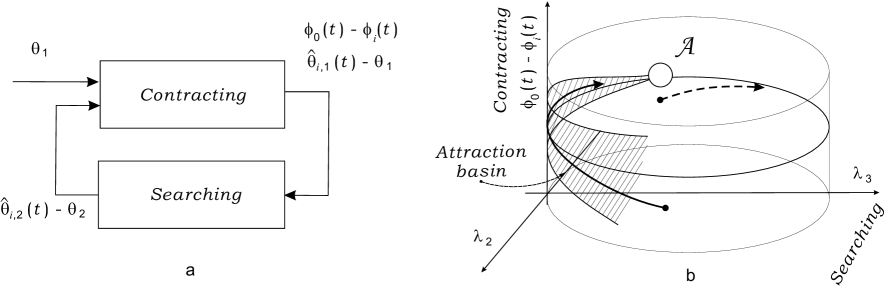
Figure 6: The interplay between temporal integration, (31a), and fast and slow adaptation (31b), (31e) in the proposed solution to the problem of invariant template matching. Panel a. Contracting dynamics corresponds to the processes of temporal integration of a template and adaptation to linearly parameterized uncertainties. Searching dynamics is due to the adaptation to nonlinearly parameterized uncertainties. Panel b. Diagram of the phase portrait of system (31a), (31b), (31e). Interaction between searching and contracting subsystems forms a weakly attracting invariant set $\mathcal{A}$. Its basin of attraction is not necessarily a neighborhood of $\mathcal{A}$. This means that some trajectories starting in a small vicinity of $\mathcal{A}$ might eventually leave its neighborhood (dashed trajectory), while trajectories starting far away from $\mathcal{A}$ might enter such neighborhoods and remain there (solid line).

We use the results from [38] to prove the emergence of weakly (Milnor) attracting sets in the system state space.

In principle, linearity of the uncertainty models in $\theta_{1}$ is not necessary to guarantee exponential stability of $\hat{\theta}_{i,1}(t)-\theta_{1}$. As has been shown in [40], exponential stability of $\hat{\theta}_{i,1}(t)-\theta_{1}$ can be ensured by the same function $\hat{\theta}_{i,1}(t)$ as in (26) if we replace $\theta_{1}f_{i}(t,\theta_{2})$ with $\tilde{f}_{i}(t,\theta_{1},\theta_{2}):\mathbb{R}_{\geq 0}\times\mathbb{R}\times\mathbb{R}\rightarrow\mathbb{R}$. Nonlinearities $\tilde{f}_{i}(t,\theta_{1},\theta_{2})$, however, should be monotone in $\theta_{1}$. In this case condition (28) is to be replaced with the following

$$D_{3}\leq\frac{\tilde{f}_{i}(t,\hat{\theta}_{i,1},\theta_{2})-\tilde{f}_{i}(t,\theta_{1},\theta_{2})}{\hat{\theta}_{i,1}-\theta_{1}}\leq D_{4},\ \forall\ \theta_{2}\in[\theta_{2,\min},\theta_{2,\max}]$$ (34)

The general line of the proof will remain unaffected by this extension.

The proposed compensatory mechanisms (24), (27) (30) are nearly optimal in terms of the dimension of the state of the whole system. Indeed, in order to track uncertain and independent $\theta_{1}$, $\theta_{2}$ two extra variables are to be introduced. This implies that the minimal dimension of state of a system which solves Problem 1 equals three. Our four-dimensional system is therefore close to the optimal configuration. Furthermore, as follows from the proof of the theorem, the dimension of the slow subsystem could be reduced to one. Thus, in principle, a minimal realization could be achieved. In this case, however, boundedness of the state for every initial condition is no longer guaranteed.

Theorem 1 establishes conditions for convergence of the trajectories of our prototype system (24), (27) (30) to an invariant set in the system state space. In particular, when matching condition (23) is met, it assures that temporal representation $\phi_{i}(t)$ of the template tracks temporal representation $\phi_{0}(t)$ of the image. In the next subsection we discuss how the similarity between these temporal representations can be detected by a system of coupled spiking oscillators.

4.2 Conditions for synchronization of coincidence detectors

Consider coincidence detectors (16), (17), (18) modeled by a system of coupled Hindmarsh-Rose oscillators. The goal of this section is to provide a constructive solution to Problem 2. First, we seek for conditions ensuring global exponential stability of the synchronization manifold of $\phi_{0}(t)=\phi_{i}(t)$ when $\phi_{i}(t)$ are identical for each $i$. We do this by showing that solutions of the system are globally bounded, and for each pair of indexes $i,j\in\{0,\dots,n\}$ there exists a differentiable positive definite function $V(x_{i},y_{i},z_{i},x_{j},y_{j},z_{j})$, ${{\partial}V}/{{\partial}x_{i}}=-{{\partial}V}/{x_{j}}$ such that $V$ grows towards infinity with distance from the synchronization manifold and for all bounded continuous $\phi_{i}(t)=\phi_{j}(t)$ the following holds:

$$\dot{V}\leq-\alpha V,\ \alpha\in\mathbb{R}_{>0}.$$ (35)

When $\phi_{i}(t)\neq\phi_{j}(t)$ equation (35) implies that

$$\dot{V}\leq-\alpha V+\frac{{\partial}V}{x_{i}}(\phi_{i}(t)-\phi_{j}(t)).$$ (36)

Then using (36) and comparison lemma [24] we show that convergence of $\phi_{i}(t)$ to $\phi_{j}(t)$ at $t\rightarrow\infty$ implies convergence of variables $x_{i}(t)$, $y_{i}(t)$, $z_{i}(t)$, $x_{j}(t)$, $y_{j}(t)$, $z_{j}(t)$ to the synchronization manifold. The formal statement of this result is provided in Theorem 2

Theorem 2

Let system (16) be given, function $\mathbf{u}$ be defined as in (17) and functions $\phi_{i}(t)$, $i\in\{0,\dots,n\}$ be bounded. Then

1) solutions of the system are bounded for all $\gamma\in\mathbb{R}_{+}$;

2) if, in addition, the following condition is satisfied

$$\gamma>\frac{1}{(n+1)\cdot a}\left(\frac{d^{2}}{2}+b^{2}\right),$$ (37)

then for all $i,j\in\{0,\dots,n\}$ condition

$$\limsup_{t\rightarrow\infty}|\phi_{i}(t)-\phi_{j}(t)|\leq\varepsilon$$

implies that

$$\begin{split}\limsup_{t\rightarrow\infty}|x_{i}(t)-x_{j}(t)|&\leq\delta(\varepsilon),\\ \limsup_{t\rightarrow\infty}|y_{i}(t)-y_{j}(t)|&\leq\delta(\varepsilon),\\ \limsup_{t\rightarrow\infty}|z_{i}(t)-z_{j}(t)|&\leq\delta(\varepsilon).\end{split}$$ (38)

where $\delta:\mathbb{R}_{+}\rightarrow\mathbb{R}_{+}$ is a monotone and vanishing at zero function.

Theorem 2 specifies the boundaries for stable synchrony in the system of coupled neural oscillators (16) as a function of the coupling strength, $\gamma$, and parameters $a$, $b$, and $d$ of a single oscillator. The last three parameters represent properties of the membrane and combined with $x_{0}$, $\varepsilon$, $s$ and $I$ completely characterize the dynamics of a single model neuron [17], ranging from single spiking to periodic or chaotic bursts.

The distinctive feature of Theorem 2 is that it is suitable for analysis of systems with external time-dependent perturbations $\phi_{i}(t)$. This property is essential for the comparison task, where the oscillators are fed with time-varying inputs and the degree of their mutual synchrony is the measure of similarity between the inputs.

While the theorem provides us with conditions for stable synchrony, it allows us to estimate the domain of values of the coupling parameter $\gamma$ corresponding to potential intermittent, itinerant[22, 23] or meta-stable regimes. In particular, as follows from Theorem 2, a necessary condition for unstable synchronization in system (16) is

$$\gamma<\frac{1}{(n+1)\cdot a}\left(\frac{d^{2}}{2}+b^{2}\right).$$ (39)

Notice that conditions (39), (37) do not depend on the “bifurcation” parameter $I$ which usually determines the type of bursting in the single oscillator. They also do not depend on the differences in the time scales defined by parameter $\varepsilon$ between the fast $x$, $y$, and slow, $z$, variables. Hence these conditions apply in a wide range of system behavior on the synchronization manifold. This advantage also has a downside, because conditions (39), (37) are too conservative. This, however, seems to be a reasonable price for invariance of criteria (39), (37) with respect to the full range of dynamical behavior of a generally nonlinear system.

5 Discussion

We provided a principled solution to the issue of invariance in the problem of template matching. The pattern recognition problem can be solved using a network of nonlinear oscillators which synchronize when mismatches in the temporal representations of image and templates converge to zero. Although the solution to the latter problem is not normative we tried to keep the number of relevant parameters at minimum. In particular the dimension of the state of a single adaptation compartment is three which is minimal for generation of spikes ranging from periodic to chaotic bursts. Moreover, conditions (39), (37) allow us to choose coupling strength $\gamma$ as single control parameter for regulating stability/instability of the synchronous activity in the network.

In this section we provide further extensions of the basic results of Theorems 1, 2, discuss possible links between the normative part of our theory and known results in vision, and provide simple illustrations how particular systems for invariant template matching can be constructed using these results.

5.1 Extension to the frequency-encoding schemes

For the sake of notational simplicity we restricted our attention to temporal representations (6), (9) of spatially sampled images. These encoding schemes can be interpreted as scanning of an image over time. Yet, the results of Section 4 apply to a broader class of encoding schemes. One example is frequency-coding used in many neural systems. Let us consider factorization (6) where in the notation $\mathcal{F}_{t}[S_{0},\mbox{\boldmath$\theta$}](x,y)$ symbol $t$ is replaced with $\nu$. In order to extend the initial encoding scheme to the domain of frequency/spike rate encoding we introduce an additional linear functional $f_{\omega}$ as follows:

$$f_{\omega}(t,\mathcal{F}_{\nu}[S_{0},\mbox{\boldmath$\theta$}])=\sum_{\nu}h(\omega_{\nu}\cdot t)\cdot f(\mathcal{F}_{\nu}[S_{0},\mbox{\boldmath$\theta$}]),$$ (40)

where $h:\mathbb{R}\rightarrow\mathbb{R}$ is a bounded periodic function, and $\omega_{\nu}$ are distinct real numbers indexed by $\nu$. Function $h(\omega_{\nu}\cdot t)$ in (40) serves as a basis or carrier function generating periodic impulses of various frequencies $\omega_{\nu}$. Thus each $\nu$-th spatial sample of the image is assigned a particular frequency, and the amplitude of the oscillation is specified by $f(\mathcal{F}_{\nu}[S_{0},\mbox{\boldmath$\theta$}])$. Temporal representation of a one-dimensional stimulus according to encoding scheme (40) is illustrated in Figure 7, panel a.

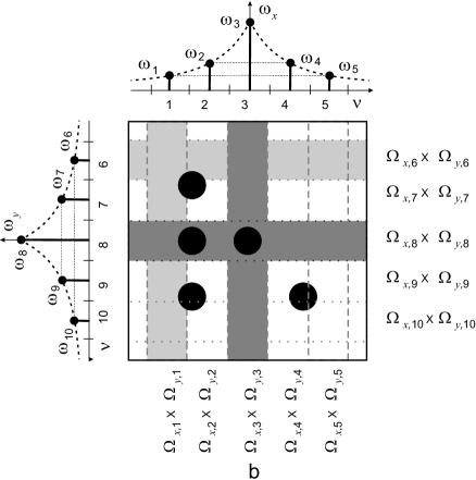
Figure 7: Panel a. Temporal representation of a spatially distributed stimulus using frequency encoding. A stimulus (upper row) $S(x)$ is spatially sampled by partitioning its domain into the union of intervals $\Omega_{i}$. For each $\Omega_{i}$ an integral $f_{i}=f(\mathcal{F}_{i})=\int_{\Omega_{i}}S(x)dx$ is calculated and a frequency $\omega_{i}$ is assigned. The resulting temporal representation (lower row) is expressed as the sum of two amplitude-modulated harmonic signals of frequencies, $\omega_{3}$, $\omega_{5}$. Panel b. Temporal representation of a two-dimensional pattern. The pattern consists of black filled circles. The image domain is partitioned into a collection of horizontal and vertical strips. Dark domains correspond to higher frequencies.

This encoding scheme is plausible to biological vision, when frequencies $\omega_{\nu}$ are ordered according to relative position of domains $\Omega_{x,\nu}$, $\Omega_{y,\nu}$ to the center of the image. This corresponds, in particular, to the receptive fields in cat retinal ganglion cells [6]. Because the functional $f_{\omega}$ is linear in $f(\mathcal{F}_{\nu}[S_{0},\mbox{\boldmath$\theta$}])$ and function $h(\omega_{\nu}\cdot t)$ is bounded for all $t$, condition (8) will be satisfied for $f_{\omega}$. Hence the conclusions of Theorem 1 apply to these systems.

5.2 Multiple representations of uncertainties

Another property of system (24), (27), (30), in addition to its ability to accommodate relevant encoding schemes such as frequency/rate and sequential/random scanning, is that each single value of $\theta_{2}\in(\theta_{2,\min},\theta_{2,\max})$ induces at least two distinct attracting sets in the extended space. Indeed

$$\lambda_{2}^{2}(t)+\lambda_{3}^{2}(t)={\mathrm{const}}=1$$

along the trajectories of (24), (27), (30) (see also the proof of Theorem 1). Hence for almost every value of $\lambda_{2}$ (except when $\lambda_{2}=\pm 1$) in the definition of $\hat{\theta}_{2}(t)$ in (30) there will always be two distinct values of $\lambda_{3}$:

$$\lambda_{3,1}=\sqrt{1-\lambda_{2}^{2}},\ \lambda_{3,2}=-\sqrt{1-\lambda_{2}^{2}}.$$

These give rise to distinct invariant sets in the system state space for the single value of $\theta_{2}$. The presence of two complementary encodings for the same figure is a plausible assumption that has been used in the perceptual organization literature to explain a range of phenomena, including perceptual ambiguity, modal and amodal completion, etc. See [43], [15] for a review. A consequence of the presence of multiple attractors corresponding to the single value of perturbation is that the time for convergence (the decision time) may change abruptly with small variations of initial conditions. The latter property is well documented in human subjects [11]. Furthermore, the presence of two attractors with different basins for a single value of perturbation will lead to asymmetric distributions of decision times, which is typically observed in human and animal reaction time data [37].

5.3 Multiple time scales for different modalities in vision

An important property of the proposed solution to the problem of invariance is that the time scales of adaptation to linearly and nonlinearly parameterized uncertainties are substantially different. This difference in time scales emerged naturally in the course of our mathematical argument as a consequence of splitting the system dynamics into a slow searching subsystem and a fast asymptotically stable one. This allowed us to prove emergence of unstable yet attracting invariant sets thus ensuring existence of a solution to the problem of invariant template matching.In particular, Theorem 1 requires that the time constants of adaptation to linearly parameterized uncertainties (for instance, unknown intensity of the image) are to be substantially smaller than the time constants of adaptation to nonlinearly parameterized uncertainties (image blur, rotation, scaling etc.). Furthermore, as follows from Table 3, the larger the difference in the time scales the higher the possible precision and the smaller the errors.

Even though the difference in time scales was motivated purely by theoretical considerations, there is strong evidence that biological systems adapt at different time scales to uncertainties from different modalities. For example, the time scale of light adaptation is within tens of milliseconds [45] while adaptation to “higher-order” modalities like rotation and image blur extends from hundreds of milliseconds to minutes [44]. In motor learning the evidence of presence of slow and fast adaptation at the time scale minutes is reported in [36]. These findings, therefore, motivate our belief that system (24), (27), (30) could serve as a simple, yet qualitatively realistic, model for adaptation mechanisms in vision, motor behavior, and decision making.

5.4 Rotation-invariant matching and mental rotation experiments

Let us illustrate how the results of Theorems 1, 2 can be applied to template matching when an object is rotated over an unknown angle and its brightness is uncertain a-priori. In order to obtain a temporal representation of the image we use the frequency-encoding scheme (40) as is illustrated in Figure 7, panel b. In particular we use the following transformation

$$\theta_{1}f_{i}(t,\theta_{2})=\theta_{1}\sum_{\nu}h(\omega_{\nu}\cdot t)\cdot f(\bar{\mathcal{F}}_{\nu}[S_{i},\theta_{2}]),$$ (41)

where $\theta_{2}$ is the rotation angle of image $S_{i}(x,y)$ around its central point, $\theta_{1}$ is the image brightness, function $h(\omega_{\nu}\cdot t)=\sin^{2}(\omega_{\nu}\cdot t)$, and

$$f(\bar{\mathcal{F}}_{\nu}[S_{i},\theta_{2}])=\int_{\Omega_{x,\nu}\times\Omega_{y,\nu}}\bar{\mathcal{F}}_{\nu}[S_{i},\theta_{2}](\xi,\gamma)d\xi d\gamma.$$

is simply an integral of the rotated image $S_{i}$ by the angle $\theta_{2}$ over the strip $\Omega_{x,\nu}\times\Omega_{y,\nu}$.

According to (24), (27), (30), (16) the recognition system (see Figure 3 for its general structure) can be described by the system of differential equations provided in Table 4. Details of their implementation, specific values of the parameters, initial conditions, and the source files of a working MATLAB Simulink model can be found in [39].

Function	Image	Template
Temporal integration	$$\dot{\phi}_{0}=-\frac{1}{\tau}\phi_{0}+k\cdot\theta_{1}f(t,\theta_{2})$$	$$\dot{\phi}_{i}=-\frac{1}{\tau}\phi_{i}+k\cdot\hat{\theta}_{1,i}f(t,\hat{\theta}_{2,i})$$
Adaptation to brightness	No	$\displaystyle\hat{\theta}_{1,i}$ $\displaystyle=$ $\displaystyle(\phi_{0}-\phi_{i})\gamma_{1}+\lambda_{i,1}$ $\displaystyle\dot{\lambda}_{i,1}$ $\displaystyle=$ $\displaystyle\frac{\gamma_{1}}{\tau}(\phi_{0}-\phi_{i})$
Adaptation to rotation	No	$\displaystyle\hat{\theta}_{2,i}$ $\displaystyle=$ $\displaystyle(\lambda_{2,i}(t)+1)\pi$ $\displaystyle\dot{\lambda}_{i,2}$ $\displaystyle=$ $\displaystyle\gamma_{2}\lambda_{i,3}\|\phi_{0}-\phi_{i}\|_{\varepsilon}$ $\displaystyle\dot{\lambda}_{i,3}$ $\displaystyle=$ $\displaystyle-\gamma_{2}\lambda_{i,2}\|\phi_{0}-\phi_{i}\|_{\varepsilon}$
Detectors of similarity	$$\begin{array}[]{ll}\dot{x}_{0}&=-a{x}_{0}^{3}+b{x}_{0}^{2}+y_{0}-z_{0}+I\\ &+u_{0}+\phi_{0}(t),\\ \dot{y}_{0}&=c-d{x}_{0}^{2}-y_{0},\\ \dot{z}_{0}&=\varepsilon(s(x_{0}+x_{0})-z_{0}),\end{array}$$	$$\begin{array}[]{ll}\dot{x}_{i}&=-a{x}_{i}^{3}+b{x}_{i}^{2}+y_{i}-z_{i}+I\\ &+u_{i}+\phi_{i}(t),\\ \dot{y}_{i}&=c-d{x}_{i}^{2}-y_{i},\\ \dot{z}_{i}&=\varepsilon(s(x_{i}+x_{i})-z_{i}),\end{array}$$
Coupling function	$u_{0}=\gamma\left(-(n+1)x_{0}+\sum_{j\neq 0}x_{j}\right)$	$u_{i}=\gamma\left(-(n+1)x_{i}+\sum_{j\neq i}x_{j}\right)$

Table 4: Equations of the system for rotation and brightness-invariant template matching.

We tested system performance for a variety of input images, in particular the class of Garner patterns [10] (see Figure 8, the first row). These patterns are widely used in the experiments with humans and therefore serve as a convenient benchmark. Their distinctive property is that their overall intensity does not vary from one pattern to another. At the same time their complexity in terms of the number of rotation and reflection symmetries can vary. In our example the first pattern has the highest complexity. The second has mid level of complexity (two symmetrical states) and the third has the lowest degree of complexity (four symmetrical states).

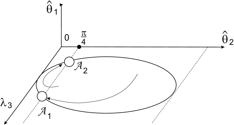
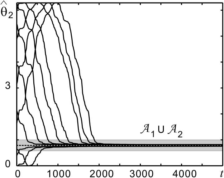
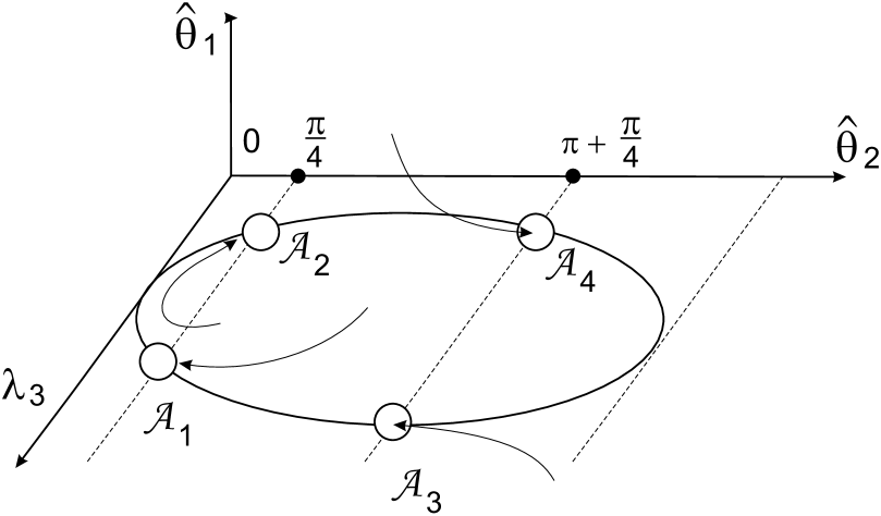
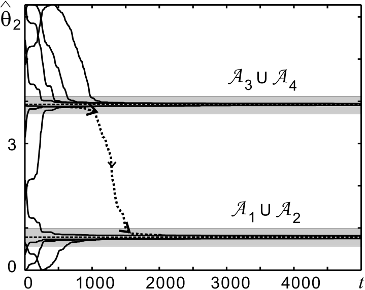
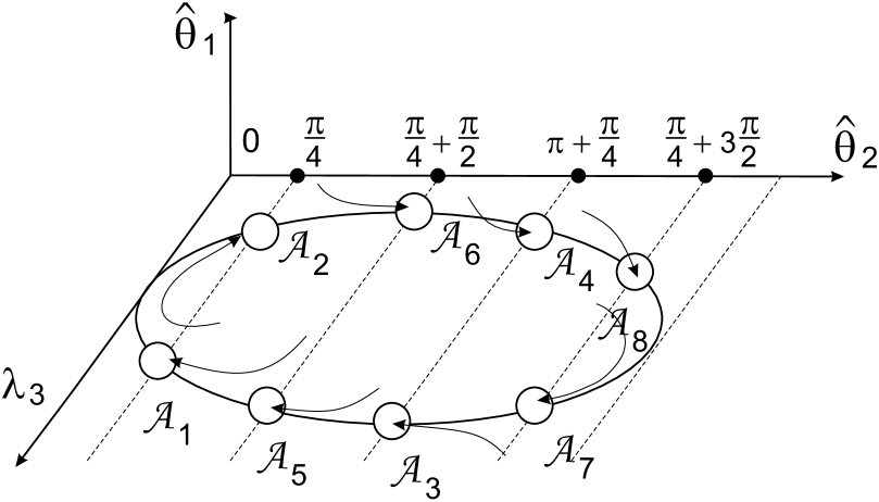
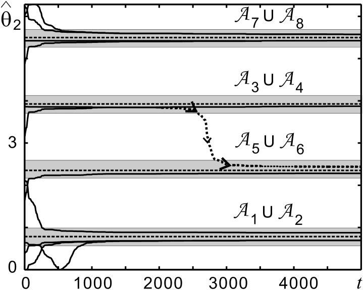
Figure 8: Template matching of Garner patterns of various complexity. The patterns (upper row) were rotated by $\pi/4$ and had various intensity. Depending on the number of their rotational symmetries they induced different number of invariant sets in the system state space: two, four and eight respectively. The diagrams of corresponding phase plots are provided in the middle row. Estimates of the rotation angle as functions of time for different initial conditions are depicted in the third row.

The second row of Figure 8 illustrates the system dynamics involved in invariant template matching for these patterns. The diagrams represent phase plots of the successful node $j$ (e.g. for the template subsystem in which the matching occurs). The third row contains trajectories of the estimates of the rotation angle $\hat{\theta}_{j,2}(t)$. Each object induces various number of invariant sets in the template subsystems. The number of these invariant sets is inversely proportional to stimulus complexity. Hence, the higher the complexity the more time the system requires to converge to an attractor. Thus the time needed for recognition increases monotonically with the stimulus complexity. This is consistent with empirical results reported in many experimental studies, for instance [25].

An additional property of our system is that it is capable of reporting multiple representations of the same object. This is indicated by the dashed trajectories in Figure 8. Even though the system parameters are chosen such that trajectories converge to an attractor, we can still observe meta-stable behavior. This is because the attractors in our system are of Milnor-type, which implies that trajectories starting in the vicinity of one attractor may actually belong to the basin of another attractor. Furthermore, it is even possible to tune the system in such a way that it will always switch from one representation to another. The latter property suggests that our simple system in Table 4 can provide a simple model for visual perception, where spontaneous switching and perceptual multi-stability are commonly observed [2], [26].

5.5 Tracking disturbances in scanning microscopes

We next consider the application of a the template-matching system with weakly attracting sets to a problem of realistic complexity. We applied our approach to the problem of tracking morphological changes in dendritic spines based on measurements received from a multiphoton scanning microscope in vitro. A distinctive property of laser microscopy is that in order to ”see” an object one needs, first, to inject it with a photo-sensitive dye (fluorophore). The particles of the fluorophore emit photons of light under external stimulation, thus illuminating an object from inside the tissue. Typical data from a two-photon microscope are provided in Figure 9.

We addressed the problem of how to register fast dynamical changes in spine geometry after application of chemical stimulation. The measurements were performed on slices. Measurements of this kind suffer from effects of photobleaching and diffusion of the dye (see Figure 9), and dependance of the scattering of the emitted light on the a-priori unknown position of the object in the slice.

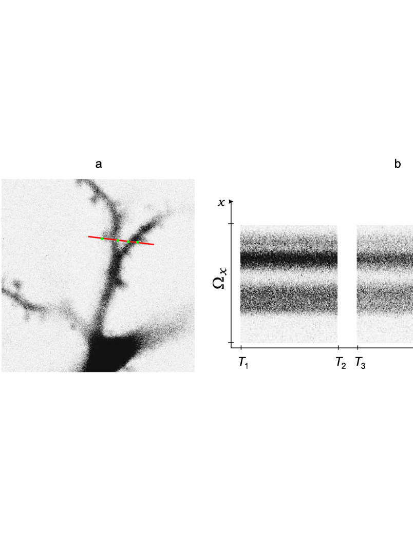
Figure 9: Typical images from the two-photon microscope. Panel $a$ shows a dendrite; the domain of scanning (red line) is in the vicinity of two spines (small protrusions on the dendrite). Size of the domain is $5.95$ micron, and speed of scanning, $v_{s}$, is $1$ pixel per $2$ micro seconds. Panel $b$ shows results of scanning as a function of time in the beginning (interval $[T_{1},T_{2}]$), in the middle of experiment (domain $[T_{3},T_{4}]$), and in the end of the experiment (domain $[T_{5},T_{6}]$).

On-line estimation and tracking the effects of photobleaching (intensity) and changes of the object position (blur) in the slice are therefore necessary.

The measured signal is already a temporal sequence, which fits nicely to our approach. An inherent feature of scanning microscopy is that the object is measured using a sequence of scans along one-dimensional domains (see Figure 9, panel $a$). Hence the objects in this case are one-dimensional mappings, and the domain $\Omega_{x}$ is an interval $\Omega_{x}=[x_{\min},x_{\max}]$. For the particular images we set $x_{\min}=1$ and $x_{\max}=176$, which corresponds to a scanning line of $176$ pixels and $5.95$ micro meters. In order to eliminate measurement noise we we consider the averaged data in the scanning line over $n$ successive subsequent trials.

The measured image, $S_{0}$, was chosen to be the averaged data along the scanning line over $n$ successive subsequent trials. The template, $S_{1}$, substituted the averaged measurements of the object at the initial time $T_{1}$.

Samples of data used to generate $S_{1}$ are provided in Figure 10, $a$. These correspond to the intensity of the emitted radiation from the object in the red part of the spectrum for the data shown in Figure 9, $b$, fragment 1.

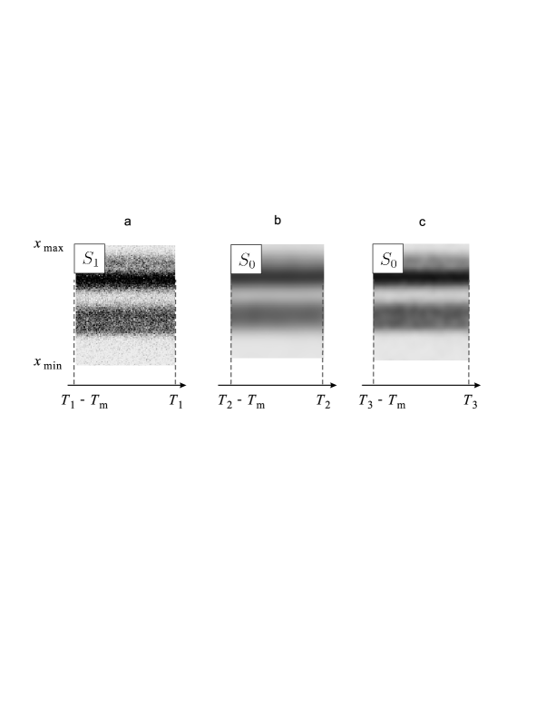
Figure 10: Data which has been used to generate the template, $S_{1}$ (panel $a$), and perturbed measurements $S_{0}$ at time instants $T_{2}$ and $T_{3}$ (panels $b$ and $c$ respectively).

Measured objects, $S_{0}$, are the averaged samples of data at the time instants $T_{i}\neq T_{1}$ (proportional to $T_{s}$). Focal distortions were simulated using conventional filters from Photoshop applied to $S_{1}$. These fragments are provided in Figure 10, panels $b$ and $c$.

Because the sources of perturbation are the effects of photobleaching (affecting brightness) and deviations in the object position in the slice (affecting scattering and leading to blurred images) the following model of uncertainty was used:

$$\begin{split}\theta_{1}f_{1}(x,\theta_{2},t)&=\theta_{1}\int_{\Omega_{x}}e^{-{{\theta}_{2}}(\xi-x(t))^{2}}S_{1}(\xi)d\xi\end{split},$$ (42)

where $x(t)$, the scanning trajectory in (42), is defined as:

$$x(t)=\left\{\begin{array}[]{ll}x_{\min}+k_{s}\cdot t&t\leq x_{\max}-x_{\min}\\ x(t-(x_{\max}-x_{\min})),&t>x_{\max}-x_{\min}\end{array}\right.,\ k_{s}=1.$$

Figures 11, 12 show the performance of our system (24), (27), (30), (16) in tracking focal/brightness perturbations for two measurements $S_{0}$.

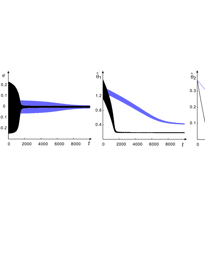
Figure 11: Trajectories $e(t)$, $\hat{\theta}_{1}(t)$, $\hat{\theta}_{2}(t)$ as functions of time. Black lines correspond to measurements in Fig. 10, panel $b$. Blue lines correspond to the data in Fig. 10, panel $c$.

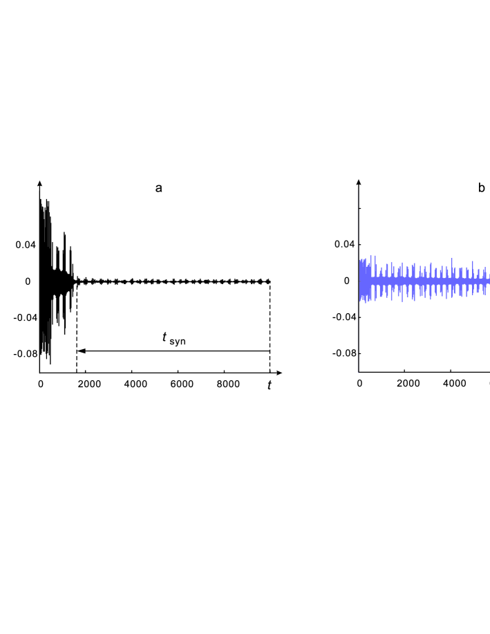
Figure 12: Plots of the synchronization errors $x_{0}(t)-x_{1}(t)$ as a function of time. Panel $a$ corresponds to the data depicted in Fig. 10, $b$. Panel $b$ corresponds to the measurements shown in Fig. 10, $c$.

Figure 11 shows the tracking of unknown modelled perturbations in the images. Figure 12 shows the synchronization errors of the detection subsystem. Symbol $t_{\mathrm{syn}}$ denotes ”synchronization time” spent in the vicinity of the invariant synchronization manifold. As follows from both figures, the system successfully tracks/reconstructs the estimates of unknown perturbations applied to the object (Fig. 11). Coincidence detectors report synchrony only when the error between the profiles of the template and object are is sufficiently small (Fig. 12). Furthermore, the physical time required for recognition on the standard PC was less than 5 seconds.

6 Conclusion

We provided a principled solution to the problem of invariant template matching on the basis of temporal coding of spatial information. We considered the problem at the levels of mathematical analysis as well as implementation of specific recognition systems. Our analysis showed that a solution to the problem requires to abandon the traditional notion of attractor, in the Lyapunov sense, for defining a system’s target set. As a substitute we proposed the concept of Milnor attracting sets. At the level of implementation we provided systems in which such attractors emerge as a result of external stimulation. These systems are endowed with mathematical rigor in the form of conditions sufficient for ensuring global convergence of trajectories to their target invariant sets. The results provided are normative in the sense that we require a minimal number of additional variables and consider as simple structures as possible.

Even though the proposed system stems from theoretical considerations, it captures qualitatively a wide range of phenomena observed in the literature on biological visual perception. These include multiple time scales for different modalities during adaptation [45], [44], [36], switching and perceptual multi-stability [2], [26], perceptual ambiguity [43], [15], empirical observations in mental rotation [25] and decision time distributions [11]. This motivates our belief that present results may contribute to the further understanding of visual perception in biological systems, including humans.

We demonstrated that the problem of invariant recognition can be solved by a simple system of ordinary differential equations with locally Lipschitz right-hand side. This result can be used as an existence proof for solving the problem of adaptive recognition by means of recurrent neural networks with fixed weights. Such systems are being used in various computational tasks [31] without any guarantee of a solution. We guarantee that solutions to realistic recognition problems (e.g. insuring invariance to rotation, blur, scaling, translation etc.) can be obtained with networks approximating our prototype system sufficiently well.

Appendix 1 Optimality of sampled representations

Consider an image $S(x,y)$ and its quantized version $S_{q}$ obtained from $S(x,y)$ by dividing domain $\Omega_{x}\times\Omega_{y}$ into the union of finite number of subsets $\Omega_{x,j}\times\Omega_{y,i}$, $\Omega_{x}=\cup_{j}^{N_{x}}\Omega_{x,j}$, $\Omega_{y}=\cup_{i}^{N_{y}}\Omega_{y,i}$. To each subset $\Omega_{x,j}\times\Omega_{y,i}$ a value is assigned, which can be thought of as the median value of $S(x,y)$ over $\Omega_{x,j}\times\Omega_{y,i}$. We represent $S_{q}$ as a function of indices $i,j$: $S_{q}(i,j)$ and assume that the value of $S_{q}(i,j)$ is quantized by a set of $N_{s}$ levels.

Consider a system of sensors which are capable of measuring image $S(x,y)$ instantaneously over the given $k$-union of subsets $\Omega_{x,j}\times\Omega_{y,i}$. The system’s cost can be naturally defined in terms of its total number of sensors. In order to measure the entire image at once the system must have at least $N_{x}N_{y}/k$ sensors, so in the optimal case its cost $C$ should equal $C(k)=N_{x}N_{y}/k$.

We estimate the amount of information contained in this sampled representation of the image. The image is represented by an $N_{x}N_{y}/k$-tuple of elements. Each element is assigned a value, say $\sigma_{i}$, from a set of $N_{s}$ levels with the given probability $p(\sigma_{i})$. Hence the entropy of the representation is

$$H(k)=-\sum_{i}p(\sigma_{i})\log\left(\frac{k}{N_{x}N_{y}}p(\sigma_{i})\right)=\log\left(\frac{N_{x}N_{y}}{k}\right)-\sum_{i}p(\sigma_{i})\log p(\sigma_{i})$$

The entropy characterizes the informational content of a representation, and function $1/H(k)$ its ambiguity.

Overall losses, $Q(k)$, therefore can be defined as a weighted sum of costs, $C(k)$, and ambiguity, $1/H(k)$:

$$Q(k)=\lambda_{1}C(k)+\lambda_{2}1/H(k),\ \lambda_{1},\lambda_{2}\in\mathbb{R}_{>0},\ k\in[1,N_{x}N_{y}]$$

Function $Q(k)$ is unimodal and increasing towards the boundaries of $k$: $k=1$, $k=N_{x}N_{y}$. This implies that the minimum of $Q(k)$ is achieved for some $k=k^{\ast}\in(1,N_{x}N_{y})$. In other words, a representation is optimal only when it is sampled, e.g. induced by a finite, yet neither complete nor elementary, partition of the domain $\Omega_{x}\times\Omega_{y}$.

Appendix 2 Proofs of the theorems

Proof of Theorem 1. We prove the theorem in three steps. First, we show that the solution of the extended system (24), (27), (30) is bounded. Second, we prove that there are constants $\rho$, $b$, $\varepsilon$ and time instant $t^{\prime}>0$ such that the following holds for system solutions:

$$\|\phi_{0}(t)-\phi_{i}(t)\|_{\varepsilon}\leq e^{-\rho(t-t_{0})}\|\phi_{0}(t_{0})-\phi_{i}(t_{0})\|_{\varepsilon}+b\|\theta_{2}-\hat{\theta}_{i,2}(\tau)\|_{\infty,[t_{0},t]}\ \ \forall\ t\geq t_{0}>t^{\prime}$$ (43)

Third, using this representation we invoke results from (our paper) and demonstrate that conclusions of the theorem follow.

1. Boundedness. To prove boundedness of solutions of the extended system in forward time let us first consider the difference $e_{i}(t)=\phi_{0}(t)-\phi_{i}(t)$. According to (24), dynamics of $e_{i}(t)$ will be defined as

$$\begin{split}\dot{e}_{i}&=-\frac{1}{\tau}e_{i}+k\left(\theta_{1}f_{i}(t,\theta_{2})-\hat{\theta}_{i,1}f_{i}(t,\hat{\theta}_{i,2})\right)+\epsilon(t)\end{split}$$ (44)

Noticing that

$$\theta_{1}f_{i}(t,\theta_{2})-\hat{\theta}_{i,1}f_{i}(t,\hat{\theta}_{i,2})=[\theta_{1}f_{i}(t,\theta_{2})-\theta_{1}f_{i}(t,\hat{\theta}_{i,2})]+[\theta_{1}f_{i}(t,\hat{\theta}_{i,2})-\hat{\theta}_{i,1}f_{i}(t,\hat{\theta}_{i,2})]$$

and denoting $\delta_{1}=\hat{\theta}_{i,1}-\theta_{1}$, $\delta_{2}(t,\theta_{1},\theta_{2},\hat{\theta}_{i,2})=\theta_{1}f_{i}(t,\theta_{2})-\theta_{1}f_{i}(t,\hat{\theta}_{i,2})$ we can rewrite (44) as follows

$$\begin{split}\dot{e}_{i}&=-\frac{1}{\tau}e_{i}-\delta_{1}[kf_{i}(t,\hat{\theta}_{i,2})]+\delta_{2}(t,\theta_{1},\theta_{2},\hat{\theta}_{i,2})k+\epsilon(t)\end{split}$$ (45)

Let us now write equations for $\hat{\theta}_{i,1}-\theta_{1}$ in (26) in differential form. To do so we differentiate variable $\hat{\theta}_{i,1}-\theta_{1}=\delta_{1}$ with respect to time, taking into account equations (44), (45):

$$\dot{\delta}_{1}=-\gamma_{1}\left(\delta_{1}[kf_{i}(t,\hat{\theta}_{i,2})]-\delta_{2}(t,\theta_{1},\theta_{2},\hat{\theta}_{i,2})k-\epsilon(t)\right)$$ (46)

Variable $\epsilon(t)$ in (46) is bounded according to (23). Let us show that $\delta_{2}(t,\theta_{1},\theta_{2},\hat{\theta}_{i,2})$ is also bounded. First of all notice that the following positive definite function

$$V_{\lambda}=0.5\left(\lambda_{2}^{2}+\lambda_{3}^{2}\right)$$

is not growing with time:

$$\dot{V}=\lambda_{2}\gamma_{2}\lambda_{3}\|\phi_{0}(t)-\phi_{i}(t)\|_{\varepsilon}-\lambda_{3}\gamma_{2}\lambda_{2}\|\phi_{0}(t)-\phi_{i}(t)\|_{\varepsilon}=0$$

Furthermore

$$\begin{split}\lambda_{2}(t)&=r\cdot\sin\left(\gamma_{2}\int_{t_{0}}^{t}\|\phi_{0}(\tau)-\phi_{i}(\tau)\|_{\varepsilon}d\tau+\varphi_{0}\right)\\ \lambda_{3}(t)&=r\cdot\cos\left(\gamma_{2}\int_{t_{0}}^{t}\|\phi_{0}(\tau)-\phi_{i}(\tau)\|_{\varepsilon}d\tau+\varphi_{0}\right),\ r,\varphi_{0}\in\mathbb{R}\end{split}$$ (47)

Choosing initial conditions $\lambda_{2}^{2}(t_{0})+\lambda_{3}^{2}(t_{0})=1$ ensures that $r=1$. Hence, according to equation (30), variable $\hat{\theta}_{i,2}$ belongs to the interval $[\theta_{2,\min},\theta_{2,\max}]$.

Consider variable $\delta_{2}(t,\theta_{1},\theta_{2},\hat{\theta}_{i,2})$:

$$\delta_{2}(t,\theta_{1},\theta_{2},\hat{\theta}_{i,2})=\theta_{1}f_{i}(t,\theta_{2})-\theta_{1}f_{i}(t,\hat{\theta}_{i,2}(t))=\theta_{1}\left(f_{i}(t,\theta_{2})-f_{i}(t,\hat{\theta}_{i,2}(t)\right)$$ (48)

Taking into account notational agreement (9), and properties (5), (8), we conclude that the following estimate holds

$$|\delta_{2}(t,\theta_{1},\theta_{2},\hat{\theta}_{i,2})|\leq\theta_{1}|f_{i}(t,\theta_{2})-f_{i}(t,\hat{\theta}_{i,2}(t)|\leq\theta_{1,\max}DD_{2}|\theta_{2}-\hat{\theta}_{i,2}(t)|$$ (49)

Given that $\hat{\theta}_{i,2}(t)\in[\theta_{2,\min},\theta_{2,\max}]$ and using (49) we can provide the following estimate for $\delta_{2}(t,\theta_{1},\theta_{2},\hat{\theta}_{i,2})$:

$$|\delta_{2}(t,\theta_{1},\theta_{2},\hat{\theta}_{i,2})|\leq\theta_{1,\max}DD_{2}|\theta_{2,\max}-\theta_{2,\min}|$$ (50)

Let us consider equality (46). According to condition 1) of the theorem, term

$$\alpha(t)=kf_{i}(t,\hat{\theta}_{i,2}(t))$$

is nonnegative and bounded from below:

$$\alpha(t)=kf_{i}(t,\hat{\theta}_{i,2}(t))\geq kD_{3},\ \forall\ t\geq 0$$ (51)

Taking into account equations (46), (51) we can estimate $|\delta_{1}(t)|$ as follows:

$$|\delta_{1}(t)|\leq e^{-\gamma_{1}\int_{t_{0}}^{t}\alpha(\tau)d\tau}|\delta_{1}(t_{0})|+\gamma_{1}e^{-\gamma_{1}\int_{t_{0}}^{t}\alpha(\tau)d\tau}\int_{t_{0}}^{t}e^{\gamma_{1}\int_{t_{0}}^{\tau}\alpha(\tau_{1})d\tau_{1}}|\epsilon(\tau)+\delta_{2}(\tau)k|d\tau$$ (52)

According to (23), (50) we have that for all $t\geq t_{0}\geq 0$

$$|\epsilon(t)+\delta_{2}(t)k|\leq\|\epsilon(\tau)+k\delta_{2}(\tau)\|_{\infty,[t_{0},t]}\leq\Delta+k\theta_{1,\max}DD_{2}|\theta_{2,\max}-\theta_{2,\min}|=M_{1}$$ (53)

Furthermore

$$\int_{t_{0}}^{t}e^{\gamma_{1}\int_{t_{0}}^{\tau}\alpha(\tau_{1})d\tau_{1}}d\tau=\frac{1}{\gamma_{1}}\left(\frac{1}{\alpha(t)}e^{\gamma_{1}\int_{t_{0}}^{t}\alpha(\tau)d\tau}-\frac{1}{\alpha(t_{0})}\right)\leq\frac{1}{\gamma_{1}D_{3}k}e^{\gamma_{1}\int_{t_{0}}^{t}\alpha(\tau)d\tau}$$ (54)

Taking into account (52), (53), and (54) we can obtain the following estimate:

$$\begin{split}|\delta_{1}(t)|\leq&e^{-\gamma_{1}kD_{4}(t-t_{0})}|\delta_{1}(t_{0})|+\frac{M_{1}}{D_{3}k}\end{split}$$ (55)

Inequality (55) proves that $\delta_{1}(t)$ is bounded.

In order to complete this step of the proof it is sufficient to show that $e_{i}(t)$ is bounded. This would automatically imply boundedness of $\phi_{i}(t)$, thus confirming boundedness of state of the extended system. To show boundedness of $e_{i}(t)$ let us write the closed-form solution of (44):

$$e_{i}(t)=e^{-\frac{(t-t_{0})}{\tau}}e_{i}(t_{0})+e^{-\frac{t}{\tau}}\int_{t_{0}}^{t}e^{\frac{\tau_{1}}{\tau}}\left(\delta_{1}(\tau_{1})\alpha(\tau_{1})+k\delta_{2}(\tau_{1})+\epsilon(\tau_{1})\right)d\tau_{1}$$ (56)

Using (53) and (55) we can derive that

$$|e_{i}(t)|\leq e^{-\frac{(t-t_{0})}{\tau}}|e_{i}(t_{0})|+M_{1}\tau\left(1+\frac{D_{4}}{D_{3}}\right)+\epsilon_{1}(t),$$ (57)

where $\epsilon_{1}(t)$ is an exponentially decaying term:

$$|\epsilon_{1}(t)|\leq e^{-\gamma_{1}kD_{3}(t-t_{0})}\left(\frac{1-e^{-\left(\frac{1}{\tau}-\gamma_{1}kD_{3}\right)(t-t_{0})}}{\frac{1}{\tau}-\gamma_{1}kD_{3}}\right)|\theta_{1}-\hat{\theta}_{i,1}(t_{0})|.$$ (58)

As follows from (47), (55), (57), (58), variables $e_{i}(t)$, $\hat{\theta}_{i,1}(t)$, $\hat{\theta}_{i,2}(t)$ are bounded. Hence state of the extended system is bounded in forward time.

2. Transformation. Let us now show that there exists a time instance $t^{\prime}$ and constants $\rho,c\in\mathbb{R}_{>0}$ such that the dynamics of $e_{i}(t)=\phi_{0}(t)-\phi_{i}(t)$ satisfies inequality (43). In order to do so we first show that term

$$\delta_{1}(t)kf_{i}(t,\hat{\theta}_{i,2}(t))$$

in (45) can be estimated as

$$|\delta_{1}(t)kf_{i}(t,\hat{\theta}_{i,2}(t))|\leq M_{2}|\theta_{2}-\hat{\theta}_{i,2}(t)|+\Delta_{2}+\epsilon_{2}(t)$$ (59)

where $M_{2}$, $\Delta_{2}$ are positive constants and $\epsilon_{2}(t)$ is a function of time which converges to zero asymptotically with time.

According to (52) the following holds

$$|\delta_{1}(t)|\leq e^{-\gamma_{1}\int_{t_{0}}^{t}\alpha(\tau)d\tau}|\delta_{1}(t_{0})|+\gamma_{1}e^{-\gamma_{1}\int_{t_{0}}^{t}\alpha(\tau)d\tau}\int_{t_{0}}^{t}e^{\gamma_{1}\int_{t_{0}}^{\tau}\alpha(\tau_{1})d\tau_{1}}|\epsilon(\tau)+\delta_{2}(\tau)k|d\tau$$

Taking into account (23), (51) we can conclude that

$$|\delta_{1}(t)|\leq e^{-\gamma_{1}kD_{3}(t-t_{0})}|\delta_{1}(t_{0})|+\frac{\Delta}{kD_{3}}+\gamma_{1}e^{-\gamma_{1}\int_{t_{0}}^{t}\alpha(\tau)d\tau}\int_{t_{0}}^{t}e^{\gamma_{1}\int_{t_{0}}^{\tau}\alpha(\tau_{1})d\tau_{1}}|\delta_{2}(\tau)k|d\tau$$ (60)

Substituting (49) into (60) results in

$$\begin{split}|\delta_{1}(t)|\leq&e^{-\gamma_{1}kD_{3}(t-t_{0})}|\delta_{1}(t_{0})|+\frac{\Delta}{kD_{3}}+\\ &\gamma_{1}e^{-\gamma_{1}\int_{t_{0}}^{t}\alpha(\tau)d\tau}\int_{t_{0}}^{t}e^{\gamma_{1}\int_{t_{0}}^{\tau}\alpha(\tau_{1})d\tau_{1}}|\theta_{2}-\hat{\theta}_{i,2}(\tau)|d\tau\cdot\left(k\theta_{1,\max}DD_{2}\right)\end{split}$$ (61)

Consider the following term in (61):

$$\int_{t_{0}}^{t}e^{\gamma_{1}\int_{t_{0}}^{\tau}\alpha(\tau_{1})d\tau_{1}}|\theta_{2}-\hat{\theta}_{i,2}(\tau)|d\tau$$ (62)

Integration of (62) by parts yields

$$\begin{split}&\int_{t_{0}}^{t}e^{\gamma_{1}\int_{t_{0}}^{\tau}\alpha(\tau_{1})d\tau_{1}}|\theta_{2}-\hat{\theta}_{i,2}(\tau)|d\tau=\frac{1}{\gamma_{1}}\left(\frac{1}{\alpha(t)}e^{\gamma_{1}\int_{t_{0}}^{t}\alpha(\tau)d\tau}|\theta_{2}-\hat{\theta}_{i,2}(t)|-\frac{|\theta_{2}-\hat{\theta}_{i,2}(t_{0})|}{\alpha(t_{0})}\right)\\ &-\frac{1}{\gamma_{1}}\int_{t_{0}}^{t}\frac{1}{\alpha(\tau)}e^{\gamma_{1}\int_{t_{0}}^{\tau}\alpha(\tau_{1})d\tau_{1}}\left(\frac{d|\theta_{2}-\hat{\theta}_{i,2}(\tau)|}{d\tau}\right)d\tau\leq\\ &\frac{1}{\gamma_{1}kD_{3}}e^{\gamma_{1}\int_{t_{0}}^{t}\alpha(\tau)d\tau}|\theta_{2}-\hat{\theta}_{i,2}(t)|+\frac{1}{\gamma_{1}kD_{3}}\int_{t_{0}}^{t}e^{\gamma_{1}\int_{t_{0}}^{\tau}\alpha(\tau_{1})d\tau_{1}}\left|\frac{d|\theta_{2}-\hat{\theta}_{i,2}(\tau)|}{d\tau}\right|d\tau\end{split}$$ (63)

Given that

$$\hat{\theta}_{2,i}=\theta_{2,\min}+\frac{\theta_{2,\max}-\theta_{2,\min}}{2}(\lambda_{2}(t)+1),$$

we can estimate the derivative $d|\theta_{2}-\hat{\theta}_{2,i}(t)|/dt$ as follows:

$$\frac{d|\theta_{2}-\hat{\theta}_{i,2}(t)|}{dt}\leq\frac{\theta_{2,\max}-\theta_{2,\min}}{2}\cdot\gamma_{2}\cdot|\phi_{0}(t)-\phi_{i}(t)|$$ (64)

Notice that the value of $|\phi_{0}(t)-\phi_{i}(t)|=e_{i}(t)$ in (64) can be estimated according to (57) as

$$|\phi_{0}(t)-\phi_{i}(t)|\leq M_{1}\tau\left(1+\frac{D_{4}}{D_{3}}\right)+\mu_{1}(t),$$

where $\mu_{1}(t)\sim\epsilon_{1}(t)+e_{i}(t)e^{-\frac{(t-t_{0})}{\tau}}$ is an asymptotically decaying term.

Hence, taking into account (54), (57), (61), (63), and (64) we may conclude that the following inequality holds

$$|\delta_{1}(t)|\leq\frac{\theta_{1,\max}DD_{2}}{D_{3}}|\theta_{2}-\hat{\theta}_{i,2}(t)|+\frac{\Delta}{D_{3}k}+\frac{\gamma_{2}}{\gamma_{1}}\frac{\theta_{1,\max}DD_{2}}{D_{3}^{2}k}\frac{\theta_{2,\max}-\theta_{2,\min}}{2}M_{1}\tau\left(1+\frac{D_{4}}{D_{3}}\right)+\mu(t)$$

where $\mu(t)$ is asymptotically vanishing term. Therefore (59) holds with the following values of $M_{2}$ and $\Delta_{2}$:

$$\begin{split}M_{2}&=\frac{k\theta_{1,\max}DD_{2}D_{4}}{D_{3}}\\ \Delta_{2}&=\frac{\gamma_{2}}{\gamma_{1}}\left[\frac{\theta_{1,\max}DD_{2}D_{4}}{(D_{3})^{2}}M_{1}\tau\left(1+\frac{D_{4}}{D_{3}}\right)\frac{\theta_{2,\max}-\theta_{2,\min}}{2}\right]+\frac{\Delta D_{4}}{D_{3}}\end{split}$$ (65)

To finalize this step of the proof consider variable $e_{i}(t)$ for $t\in[t_{1},\infty]$, $t_{1}\geq t_{0}$. According to (56), (49) we have that

$$\begin{split}|e_{i}(t)|&\leq e^{-\frac{t-t_{1}}{\tau}}|e_{i}(t_{1})|+\tau M_{2}\|\theta_{2}-\hat{\theta}_{i,2}(t)\|_{\infty,[t_{1},t]}+\\ &\tau\Delta_{2}\left(1-e^{-\frac{(t-t_{1})}{\tau}}\right)+\tau\|\epsilon_{2}(t)\|_{\infty,[t_{1},\infty]}\left(1-e^{-\frac{(t-t_{1})}{\tau}}\right)+\\ &\tau k\theta_{1,\max}DD_{2}\|\theta_{2}-\hat{\theta}_{i,2}(t)\|_{\infty,[t_{1},t]}+\tau\Delta\left(1-e^{-\frac{(t-t_{1})}{\tau}}\right)\end{split}$$ (66)

Regrouping terms in (66) yields:

$$\begin{split}|e_{i}(t)|-\tau\left(\Delta_{2}+\Delta+\|\epsilon_{2}(t)\|_{\infty,[t_{1},\infty]}\right)&\leq e^{-\frac{t-t_{1}}{\tau}}\left(|e_{i}(t_{1})|-\tau\left(\Delta_{2}+\Delta+\|\epsilon_{2}(t)\|_{\infty,[t_{1},\infty]}\right)\right)\\ &+\tau(M_{2}+k\theta_{1,\max}DD_{2})\|\theta_{2}-\hat{\theta}_{i,2}(t)\|_{\infty,[t_{1},t]}\end{split}$$

Denoting

$$\Delta^{\prime}=\tau\left(\Delta_{2}+\Delta+\|\epsilon_{2}(t)\|_{\infty,[t_{1},\infty]}\right)$$ (67)

we can obtain

$$\begin{split}|e_{i}(t)|-\Delta^{\prime}&\leq e^{-\frac{t-t_{1}}{\tau}}\left(|e_{i}(t_{1})|-\Delta^{\prime}\right)+\tau(M_{2}+k\theta_{1,\max}DD_{2})\|\theta_{2}-\hat{\theta}_{i,2}(t)\|_{\infty,[t_{1},t]}\\ &\leq e^{-\frac{t-t_{1}}{\tau}}\|e_{i}(t_{1})\|_{\Delta^{\prime}}+\tau(M_{2}+k\theta_{1,\max}DD_{2})\|\theta_{2}-\hat{\theta}_{i,2}(t)\|_{\infty,[t_{1},t]}\end{split}$$ (68)

Given that

$$\|e_{i}(t)\|_{\Delta^{\prime}}=\left\{\begin{array}[]{ll}|e_{i}(t)|-\Delta^{\prime},&|e_{i}(t)|>\Delta^{\prime}\\ 0,&|e_{i}(t)|\leq\Delta^{\prime}\end{array}\right.$$

and taking into account inequality (68), we can conclude that

$$\|e_{i}(t)\|_{\Delta^{\prime}}\leq e^{-\frac{t-t_{1}}{\tau}}\|e_{i}(t_{1})\|_{\Delta^{\prime}}+\tau(M_{2}+k\theta_{1,\max}DD_{2})\|\theta_{2}-\hat{\theta}_{i,2}(t)\|_{\infty,[t_{1},t]}$$ (69)

Because equations (66) – (69) hold for any $t_{1}\in(t_{0},\infty]$ and that

$$\limsup_{{t_{1}}\rightarrow\infty}\|\epsilon_{2}(t)\|_{\infty,[t_{1},\infty]}=0$$

for every

$$\varepsilon>\tau(\Delta+\Delta_{2})$$

there exists a time instant $t^{\prime}\geq t_{0}$ such that the following inequality is satisfied

$$\|e_{i}(t)\|_{\varepsilon}\leq e^{-\frac{t-t_{1}}{\tau}}\|e_{i}(t_{1})\|_{\varepsilon}+\tau(M_{2}+k\theta_{1,\max}DD_{2})\|\theta_{2}-\hat{\theta}_{i,2}(t)\|_{\infty,[t_{1},t]}$$ (70)

for all $t\geq t_{1}\geq t^{\prime}$. This proves (43) for $\rho=\frac{1}{\tau}$, $b=\tau(M_{2}+k\theta_{1,\max}DD_{2})$. Hence the second step of the proof is completed.

3. Convergence. In order to prove convergence we employ the following result from [38]:

Lemma 1 (Corollary 3 in [38])

Consider the following interconnection of two systems:

$$\begin{split}\mathcal{S}_{a}:\ &\left\|\mathbf{x}(t)\right\|_{\mathcal{A}}\leq\left\|\mathbf{x}(t_{0})\right\|_{\mathcal{A}}\cdot\beta_{t}(t-t_{0})+c\cdot\|h(\tau)\|_{\infty,[t_{0},t]},\ \mathbf{x}:\mathbb{R}_{\geq 0}\rightarrow\mathbb{R}^{n}\\ \mathcal{S}_{w}:\ &\int_{t_{0}}^{t}\underline{\gamma}\left\|\mathbf{x}(\tau)\right\|_{\mathcal{A}}d\tau\leq h(t_{0})-h(t)\leq\int_{t_{0}}^{t}\bar{\gamma}\left\|\mathbf{x}(\tau)\right\|_{\mathcal{A}}d\tau,\ \forall\ t\geq t_{0},\ t_{0}\in\mathbb{R}_{+}\end{split}$$ (71)

where the systems $\mathcal{S}_{a}$, $\mathcal{S}_{w}$ are forward-complete, function $\beta_{t}:\mathbb{R}_{\geq 0}\rightarrow\mathbb{R}_{\geq 0}$ is strictly monotone and decreases to zero as $t\rightarrow\infty$. Let us suppose that the following condition is satisfied

$$\bar{\gamma}\cdot c\cdot\mathcal{G}<1,$$ (72)

where

$$\mathcal{G}=\beta_{t}^{-1}\left(\frac{d}{\kappa}\right)\frac{k}{k-1}\left(\beta_{t}(0)\left(1+\frac{\kappa}{1-d}\right)+1\right)$$

for some $d\in(0,1)$, $\kappa\in(1,\infty)$.

Then there exists a set $\Omega_{\gamma}$ of initial conditions corresponding to trajectories $\mathbf{x}(t)$, $h(t)$ such that

$$\limsup_{t\rightarrow\infty}\left\|\mathbf{x}(t)\right\|_{\mathcal{A}}\leq c\cdot h(t_{0});\ \ h(t)\in[0,h(t_{0})]\ \forall\ t\geq t_{0}$$

In particular, $\Omega_{\gamma}$ contains the following domain

$$\begin{split}\left\|\mathbf{x}(t_{0})\right\|_{\mathcal{A}}\leq\frac{1}{\beta_{t}(0)}\left[\frac{1}{\bar{\gamma}}\left(\beta_{t}^{-1}\left(\frac{d}{\kappa}\right)\right)^{-1}\frac{k-1}{k}-c\left(\beta_{t}(0)\left(1+\frac{\kappa}{1-d}\right)+1\right)\right]h(t_{0}).\end{split}$$

In order to apply Lemma 1 we need to further transform equations (47), (70) and

$$\hat{\theta}_{i,2}(t)=\theta_{2,\min}+\frac{\theta_{2,\max}-\theta_{2,\min}}{2}(\lambda_{2}(t)+1)$$ (73)

into the form of equation (71). First, we notice that for every $\theta_{2}\in[\theta_{2,\min},\theta_{2,\max}]$ there always exists a real number $\lambda^{\ast}\in[-1,1]$ such that

$$\theta_{2}=\theta_{2,\min}+\frac{\theta_{2,\max}-\theta_{2,\min}}{2}(\lambda_{2}^{\ast}+1)$$

Hence, denoting

$$c=\tau(M_{2}+k\theta_{1,\max}DD_{2})\frac{\theta_{2,\max}-\theta_{2,\min}}{2}$$

and using (70) we ascertain that the following holds for solutions of system (24), (27), (30):

$$\|e_{i}(t)\|_{\varepsilon}\leq e^{-\frac{t-t_{1}}{\tau}}\|e_{i}(t_{1})\|_{\varepsilon}+c\|\lambda_{2}^{\ast}-\lambda_{2}(t)\|_{\infty,[t_{1},t]}$$ (74)

for $\varepsilon>\tau(\Delta+\Delta_{2})$, and $t\geq t_{1}\geq t^{\prime}$.

Consider the difference $\lambda_{2}^{\ast}-\lambda_{2}(t)$. According to (47) we have

$$|\lambda_{2}^{\ast}-\lambda_{2}(t)|\leq|\sigma^{\ast}-\int_{t_{1}}^{t}\gamma_{2}\|e_{i}(\tau)\|_{\varepsilon}-\varphi_{0}|,\ \lambda_{2}^{\ast}=\sin(\sigma^{\ast})$$ (75)

Denoting

$$h(t)=\sigma^{\ast}-\int_{t_{1}}^{t}\gamma_{2}\|e_{i}(\tau)\|_{\varepsilon}-\varphi_{0}$$ (76)

and taking into account (74), we therefore obtain the following equations

$$\begin{split}\|e_{i}(t)\|_{\varepsilon}&\leq e^{-\frac{t-t_{1}}{\tau}}\|e_{i}(t_{1})\|_{\varepsilon}+c\|h(t)\|_{\infty,[t_{1},t]}\\ h(t_{1})-h(t)&=\int_{t_{1}}^{t}\gamma_{2}\|e_{i}(\tau)\|_{\varepsilon}d\tau\end{split}$$ (77)

Equations (77) are a particular case of equations (71) to which Lemma 1 applies. In system (77), however, function $\beta_{t}(t)$ is defined as $\beta_{t}(t)=e^{-\frac{t}{\tau}}$. Hence

$$\beta_{t}^{-1}(t)=-\tau\ln(t)$$

Therefore, according to Lemma 1, satisfying inequality

$$\gamma_{2}\cdot c\cdot\tau\ln\left(\frac{\kappa}{d}\right)\frac{k}{k-1}\left(\left(1+\frac{\kappa}{1-d}\right)+1\right)<1$$ (78)

for some $\kappa\in(1,\infty)$, $d\in(0,1)$ ensures existence of initial conditions $e_{i}(t_{1})$, $h(t_{1})$ such that $h(t)$ is bounded. Given that

$$\min_{\kappa\in(1,\infty),,d\in(0,1)}\ln\left(\frac{\kappa}{d}\right)\frac{k}{k-1}\left(\left(1+\frac{\kappa}{1-d}\right)+1\right)\approx 15.6886<16$$

we can rewrite condition (78) in a more conservative, yet simpler form:

$$\gamma_{2}\cdot c\cdot\tau<\frac{1}{16}$$

Taking into account notations (65), (76) we can rewrite this inequality as follows:

$$\gamma_{2}<\left(\frac{1}{4\tau}\right)^{2}\left[k\theta_{1,\max}DD_{2}\left(1+\frac{D_{4}}{D_{3}}\right)\left(\frac{\theta_{2,\max}-\theta_{2,\min}}{2}\right)\right]^{-1}$$

Notice that because the function $\sin(\cdot)$ is periodic, the value of $\sigma^{\ast}$ in (75) and, subsequently the value of $h(t_{1})$, can be chosen arbitrarily large. Hence for any finite $e_{i}(t_{1})$ and $\varphi_{0}$ there will always exist $\sigma^{\ast}$ and $h(t_{1})$ such that variable $h(t)$ is bounded.

Taking into account that $h(t)$ is monotone and bounded, we can conclude that according to the Bolzano-Weierstrass theorem function $h(t)$ has a limit in $[0,h(t_{1})]$:

$$\exists h^{\ast}\in[0,h(t_{1})]:\ \lim_{t\rightarrow\infty}h(t)=h^{\ast}.$$

This in turn implies that

$$\lim_{t\rightarrow\infty}\int_{t_{1}}^{t}\gamma_{2}\|e_{i}(\tau)\|_{\varepsilon}d\tau=\sigma^{\ast}-\varphi_{0}-h^{\ast}<\infty$$

Therefore

$$\exists\ \theta_{2}^{\prime}\in[\theta_{2,\min},\theta_{2,\max}]:\ \lim_{t\rightarrow\infty}\hat{\theta}_{i,2}(t)=\theta_{2,\min}+\frac{\theta_{2,\max}-\theta_{2,\min}}{2}(\sin(\sigma^{\ast}-\varphi_{0}-h^{\ast})+1)=\theta_{2}^{\prime}$$

Moreover, because $\|e_{i}(t)\|_{\varepsilon}$ is uniformly continuous in $t$, convergence of $\|e_{i}(t)\|_{\varepsilon}$ to zero as $t\rightarrow\infty$ follows immediately from Barbalat’s lemma. The theorem is proven.

Proof of Theorem 2. The proof consists of three major steps. First, we show that single Hindmarsh-Rose oscillator is a semi-passive system with radially unbounded storage function [30]. In other words, system:

$$\begin{split}\dot{x}&=-ax^{3}+bx^{2}+y-z+I+u\\ \dot{y}&=c-dx^{2}-y\\ \dot{z}&=\varepsilon(s(x+x_{0})-z),\ \ a,b,c,d,\varepsilon,s>0\end{split}$$ (79)

obeys the following inequality

$$V(x(t),y(t),z(t))-V(x(0),y(0),z(0))\leq\int_{0}^{t}x(\tau)u(\tau)-H(x(\tau),y(\tau),z(\tau))d\tau.$$ (80)

where function $H(\cdot)$ is non-negative outside a ball in $\mathbb{R}^{3}$, and function $V$ is positive definite and radially unbounded. Second, similar to [30], we show that semi-passivity of (79) implies that solutions of the coupled system (16) are bounded. Third, for an arbitrary pair $(i,j)$ of the oscillators we present a nonnegative function such that properties (35), (36) hold for sufficiently large values of $\gamma$. Then we use the comparison lemma [24] to complete the proof.

1) Semi-passivity of the Hindmash-Rose oscillator. Let us consider the following class of functions $V$:

$$V(x,y,z)=\frac{1}{2}\left(c_{1}x^{2}+c_{2}y^{2}+c_{3}z^{2}\right)$$

Then showing existence of a function $V$ from the above class which, in addition satisfies inequality

$$\dot{V}\leq xu-H(x,y,z),$$ (81)

where $H$ is non-negative outside some ball in $\mathbb{R}^{3}$, would imply semi-passivity of (79).

Consider the time-derivative of $V$:

$$\dot{V}(x,y,z)=-c_{1}ax^{4}-c_{2}dx^{2}y-c_{2}y^{2}+c_{1}xy\\ -c_{3}\varepsilon z^{2}+(c_{3}\varepsilon s-c_{1})xz+c_{1}bx^{3}+c_{1}Ix+c_{2}cy+c_{3}\varepsilon sx_{0}z+c_{1}xu.$$ (82)

Let us rewrite (82) such that the cross terms $xy$, $xz$ and $x^{2}y$ are expressed in terms of the powers of $x,y,z$ and their sums. In order to do this we employ the following three equalities:

$$-c_{2}y^{2}+c_{1}xy=-c_{2}{\lambda_{2}}y^{2}-c_{2}(1-{\lambda_{2}})\Big{(}y-\frac{c_{1}}{2c_{2}(1-{\lambda_{2}})}x\Big{)}^{2}+\frac{{c_{1}}^{2}}{4c_{2}(1-{\lambda_{2}})}x^{2}$$ (83)

$$-c_{3}\varepsilon z^{2}+(c_{3}\varepsilon s-c_{1})xz=-c_{3}\varepsilon{\lambda_{3}}z^{2}-c_{3}\varepsilon(1-{\lambda_{3}})\Big{(}z-\frac{c_{3}\varepsilon s-c_{1}}{2c_{3}\varepsilon(1-{\lambda_{3}})}x\Big{)}^{2}+\frac{(c_{3}\varepsilon s-c_{1})^{2}}{4c_{3}\varepsilon(1-{\lambda_{3}})}x^{2}$$ (84)

$$-c_{1}ax^{4}-c_{2}dx^{2}y=-c_{1}a{\lambda_{1}}x^{4}-c_{1}a(1-{\lambda_{1}})\Big{(}x^{2}+\frac{c_{2}d}{2c_{1}a(1-{\lambda_{1}})}y\Big{)}^{2}+\frac{(c_{2}d)^{2}}{4c_{1}a(1-{\lambda_{1}})}y^{2}$$ (85)

In what follows we will assume that constants ${\lambda_{1}}$, ${\lambda_{2}}$ and ${\lambda_{3}}$ in (83)–(85) are chosen arbitrarily in the interval $(0,1)$: $0<{\lambda_{i}}<1,\;i=1,2,3$.

Taking equalities (83)–(85) into account, we can rewrite the time derivative of $V$ (equation (82)) in the following form:

$$\dot{V}(x,y,z)=-c_{1}a(1-{\lambda_{1}})\Big{(}x^{2}+\frac{c_{2}d}{2c_{1}a(1-{\lambda_{1}})}y\Big{)}^{2}-c_{2}(1-{\lambda_{2}})\Big{(}y-\frac{c_{1}}{2c_{2}(1-{\lambda_{2}})}x\Big{)}^{2}+\\ -c_{3}\varepsilon(1-{\lambda_{3}})\Big{(}z-\frac{c_{3}\varepsilon s-c_{1}}{2c_{3}\varepsilon(1-{\lambda_{3}})}x\Big{)}^{2}-c_{2}\Big{(}{\lambda_{2}}-\frac{c_{2}d^{2}}{4c_{1}a(1-{\lambda_{1}})}\Big{)}y^{2}+c_{2}cy+\\ -c_{3}\varepsilon{\lambda_{3}}z^{2}+c_{3}\varepsilon sx_{0}z-c_{1}a{\lambda_{1}}x^{4}+c_{1}bx^{3}+\Big{(}\frac{{c_{1}}^{2}}{4c_{2}(1-{\lambda_{2}})}+\frac{(c_{3}\varepsilon s-c_{1})^{2}}{4c_{3}\varepsilon(1-{\lambda_{3}})}\Big{)}x^{2}+c_{1}Ix+c_{1}xu$$ (86)

Our goal is to express the right-hand side of (86) in the following form:

$$\dot{V}\leq c_{1}xu+\left(M-H_{0}(x,y,z)\right),$$ (87)

where $H_{0}(x,y,z)$ is a radially unbounded nonnegative function outside a ball in $\mathbb{R}^{3}$, and $M$ is a constant. For this reason we select constants $\lambda_{2},c_{2}$ in (81) as follows:

$${\lambda_{2}}-\frac{c_{2}d^{2}}{4c_{1}a(1-{\lambda_{1}})}>0,\ \ \mathrm{or}\ \ \frac{c_{2}}{c_{1}}<\frac{4a{\lambda_{2}}(1-{\lambda_{1}})}{d^{2}}.$$ (88)

Noticing that

$$-c_{2}\Big{(}{\lambda_{2}}-\frac{c_{2}d^{2}}{4c_{1}a(1-{\lambda_{1}})}\Big{)}y^{2}+c_{2}cy=\\ -c_{2}\big{(}{\lambda_{2}}-\frac{c_{2}d^{2}}{4c_{1}a(1-{\lambda_{1}})}\big{)}\Big{(}y-\frac{2cc_{1}a(1-{\lambda_{1}})}{4{\lambda_{2}}c_{1}a(1-{\lambda_{1}})-c_{2}d^{2}}\Big{)}^{2}+\frac{c_{1}c_{2}c^{2}a(1-{\lambda_{1}})}{4{\lambda_{2}}c_{1}a(1-{\lambda_{1}})-c_{2}d^{2}}$$ (89)

$$-c_{3}\varepsilon{\lambda_{3}}z^{2}+c_{3}\varepsilon sx_{0}z=-c_{3}\varepsilon{\lambda_{3}}\Big{(}z-\frac{sx_{0}}{2{\lambda_{3}}}\Big{)}^{2}+\frac{c_{3}\varepsilon s^{2}{x_{0}}^{2}}{4{\lambda_{3}}}$$ (90)

proves representation (87) for any fixed $x=\mathrm{const}$. In order to show that (87) holds with respect to the complete set of variables, e.g. $(x,y,z)$ we use the following sequence of equalities:

$$-c_{1}a{\lambda_{1}}x^{4}+c_{1}bx^{3}+\Big{(}\frac{{c_{1}}^{2}}{4c_{2}(1-{\lambda_{2}})}+\frac{(c_{3}\varepsilon s-c_{1})^{2}}{4c_{3}\varepsilon(1-{\lambda_{3}})}\Big{)}x^{2}+c_{1}Ix=(\mathrm{see\ \ notations\ \ below})\\ -a_{0}x^{4}+a_{1}x^{3}+a_{2}x^{2}+a_{3}x+a_{4}=\\ -b_{0}x^{4}-\big{(}x-b_{1}\big{)}^{4}+b_{2}x^{2}+b_{3}x+b_{4}=\\ -b_{0}x^{4}-\big{(}x-b_{1}\big{)}^{4}+\big{(}b_{2}+d_{0}\big{)}x^{2}-d_{0}\big{(}x-d_{1}\big{)}^{2}+d_{2}=\\ -b_{0}\big{(}x^{2}-e_{0}\big{)}^{2}-\big{(}x-b_{1}\big{)}^{4}-d_{0}\big{(}x-d_{1}\big{)}^{2}+e_{1}$$ (91)

with

$$\begin{split}a_{0}&=c_{1}a{\lambda_{1}},\ a_{1}=c_{1}b,\ a_{2}=\frac{{c_{1}}^{2}}{4c_{2}(1-{\lambda_{2}})}+\frac{(c_{3}\varepsilon s-c_{1})^{2}}{4c_{3}\varepsilon(1-{\lambda_{3}})}\\ a_{3}&=c_{1}I,\ a_{4}=0\ b_{0}=a_{0}-1,\ b_{1}=\tfrac{1}{4}a_{1},\ b_{2}=a_{2}+\tfrac{3}{8}{a_{1}}^{2},\ b_{3}=a_{3}-\tfrac{1}{16}{a_{1}}^{3},\ b_{4}=a_{4}+\tfrac{1}{256}{a_{1}}^{4}\\ d_{0}&=1,\ d_{1}=\frac{b_{3}}{2d_{0}},\ d_{2}=b_{4}+{d_{1}}^{2}d_{0},\ e_{0}=\frac{b_{2}+d_{0}}{2b_{0}},\ e_{1}=d_{2}+b_{0}{e_{0}}^{2}\end{split}$$ (92)

Notice that we want the value of $b_{0}$ in (91), (92) be positive. Hence the value of

$$a_{0}=c_{1}a{\lambda_{1}}$$

should be greater than $1$. This can be ensured by choosing the value of $c_{1}$ in (81) to be sufficiently large. As a result of this choice, taking restrictions (88) into account, we conclude that the value of $c_{2}$ in (81) must be sufficiently small, e.g. satisfy the following inequality:

$${c_{2}}<c_{1}\frac{4a{\lambda_{2}}(1-{\lambda_{1}})}{d^{2}}.$$

The value for $d_{0}$ can be chosen arbitrarily, here $d_{0}=1$.

Time-derivative $\dot{V}$ can now be written as follows

$$\dot{V}(x,y,z)=-c_{1}a(1-{\lambda_{1}})\Big{(}x^{2}+\frac{c_{2}d}{2c_{1}a(1-{\lambda_{1}})}y\Big{)}^{2}\\ -c_{3}\varepsilon(1-{\lambda_{3}})\Big{(}z-\frac{c_{3}\varepsilon s-c_{1}}{2c_{3}\varepsilon(1-{\lambda_{3}})}x\Big{)}^{2}\\ -c_{2}(1-{\lambda_{2}})\Big{(}y-\frac{c_{1}}{2c_{2}(1-{\lambda_{2}})}x\Big{)}^{2}\\ -c_{3}\varepsilon{\lambda_{3}}\Big{(}z-\frac{sx_{0}}{2{\lambda_{3}}}\Big{)}^{2}+\frac{c_{3}\varepsilon s^{2}{x_{0}}^{2}}{4{\lambda_{3}}}+\\ -c_{2}\big{(}{\lambda_{2}}-\frac{c_{2}d^{2}}{4c_{1}a(1-{\lambda_{1}})}\big{)}\Big{(}y-\frac{2cc_{1}a(1-{\lambda_{1}})}{4{\lambda_{2}}c_{1}a(1-{\lambda_{1}})-c_{2}d^{2}}\Big{)}^{2}+\frac{c_{1}c_{2}c^{2}a(1-{\lambda_{1}})}{4{\lambda_{2}}c_{1}a(1-{\lambda_{1}})-c_{2}d^{2}}+\\ -b_{0}\big{(}x^{2}-e_{0}\big{)}^{2}-\big{(}x-b_{1}\big{)}^{4}-d_{0}\big{(}x-d_{1}\big{)}^{2}+e_{1}+c_{1}xu$$ (93)

It is straightforward to see that expression (93) is of the form (87), where

$$\begin{split}H_{0}(x,y,z)=&\>c_{1}a(1-{\lambda_{1}})\Big{(}x^{2}+\frac{c_{2}d}{2c_{1}a(1-{\lambda_{1}})}y\Big{)}^{2}+c_{3}\varepsilon(1-{\lambda_{3}})\Big{(}z-\frac{c_{3}\varepsilon s-c_{1}}{2c_{3}\varepsilon(1-{\lambda_{3}})}x\Big{)}^{2}\\ &+c_{2}(1-{\lambda_{2}})\Big{(}y-\frac{c_{1}}{2c_{2}(1-{\lambda_{2}})}x\Big{)}^{2}+c_{3}\varepsilon{\lambda_{3}}\Big{(}z-\frac{sx_{0}}{2{\lambda_{3}}}\Big{)}^{2}\\ &+c_{2}\big{(}{\lambda_{2}}-\frac{c_{2}d^{2}}{4c_{1}a(1-{\lambda_{1}})}\big{)}\Big{(}y-\frac{2cc_{1}a(1-{\lambda_{1}})}{4{\lambda_{2}}c_{1}a(1-{\lambda_{1}})-c_{2}d^{2}}\Big{)}^{2}\\ &+b_{0}\big{(}x^{2}-e_{0}\big{)}^{2}+\big{(}x-b_{1}\big{)}^{4}+d_{0}\big{(}x-d_{1}\big{)}^{2}\end{split}$$

$$M=\frac{c_{3}\varepsilon s^{2}{x_{0}}^{2}}{4{\lambda_{3}}}+\frac{c_{1}c_{2}c^{2}a(1-{\lambda_{1}})}{4{\lambda_{2}}c_{1}a(1-{\lambda_{1}})-c_{2}d^{2}}+e_{1}$$

Let us denote

$$H_{1}(x,y,z)=H_{0}-M$$

and rewrite (87) as

$$\dot{V}\leq c_{1}xu-H_{1}(x,y,z)$$

Function $H_{1}(x,y,z)$ is radially unbounded. Furthermore, it is non-negative outside a ball in $\mathbb{R}^{3}$. Hence choosing

$$V^{\ast}(x,y,z)=\frac{1}{c_{1}}V(x,y,z)$$

we assure existence of (radially unbounded) positive definite $V^{\ast}(x,y,z)$ such that

$$\dot{V}^{\ast}\leq xu-\frac{H_{1}(x,y,z)}{c_{1}},$$ (94)

where $H_{1}(x,y,z)/c_{1}$ is radially unbounded and non-negative outside a ball in $\mathbb{R}^{3}$. Thus, according to (81), semi-passivity of the Hindmarsh-Rose system follows.

2) Boundedness of the solutions. We aim to prove that boundedness of $\phi_{i}(t)$, $i\in\{0,\dots,n\}$ implies boundedness of the state of the coupled system. Without loss of generality we assume that

$$\|\phi_{i}(\tau)\|_{\infty,[0,\infty]}\leq D_{\phi}$$

Let us denote

$$V_{i}=V^{\ast}(x_{i},y_{i},z_{i}),\ \ H_{1,i}=\frac{1}{c_{1}}H_{1}(x_{i},y_{i},z_{i}).$$

Consider the following function

$$V_{\Sigma}(\mathbf{x},\mathbf{y},\mathbf{z})=\rho\left(\sum_{i=0}^{n}V_{i}(x_{i},y_{i},z_{i}),C\right).$$ (95)

where $\mathbf{x}={\mathrm{col}}(x_{0},\dots,x_{n})$, $\mathbf{y}={\mathrm{col}}(y_{0},\dots,y_{n})$, $\mathbf{z}={\mathrm{col}}(z_{0},\dots,z_{n})$ and

$$\rho(s,C)=\left\{\begin{array}[]{cl}s-C,&\ s\geq C\\ 0,&s<C\end{array}\right.$$

Function $V_{\Sigma}$ is nonnegative for any $C\in\mathbb{R}$ and, furthermore, is radially unbounded. Hence, its boundedness for some $C\in\mathbb{R}$ implies boundedness of $x_{i}$, $y_{i}$, $z_{i}$, $i\in\{0,\dots,n\}$.

Let us pick $C\in\mathbb{R}$ such that interior of the domain

$$\Omega_{C}=\{\mathbf{x},\mathbf{y},\mathbf{z}\in\mathbb{R}\ \left|\right.\ \sum_{i=0}^{n}V_{i}(x_{i},y_{i},z_{i})\leq C\}$$

contains the domain

$$\sum_{i=0}^{n}H_{1,i}(x_{i},y_{i},z_{i})-\kappa x_{i}^{2}<M_{i},\ M_{i}\in\mathbb{R}_{>0},\ \kappa\in\mathbb{R}_{>0}$$

where $M_{i}$ is an arbitrarily large and $\kappa$ is an arbitrary small positive constant. In other words the following implication holds:

$$\sum_{i=0}^{n}V_{i}(x_{i},y_{i},z_{i})\geq C\Rightarrow\sum_{i=0}^{n}H_{1,i}(x_{i},y_{i},z_{i})-\kappa x_{i}^{2}\geq M_{i}$$ (96)

Such $C$ always exists because $H_{1,i}(x_{i},y_{i},z_{i})-\kappa x_{i}^{2}$ can be expressed as a sum of a nonnegative quadratic form in $x_{i},y_{i},z_{i}$ and non-negative functions of the higher order plus a constant, and $V_{i}(x_{i},y_{i},z_{i})$ is a positive-definite quadratic form.

Consider time-derivative of function $V_{\Sigma}(\mathbf{x},\mathbf{y},\mathbf{z})$. According to (95), (94) it is zero for all $\mathbf{x},\mathbf{y},\mathbf{z}\in\Omega_{C}$, and satisfies the following inequality otherwise:

$$\dot{V}_{\Sigma}\leq\sum x_{i}u_{i}-\sum_{i=0}^{n}H_{1,i}(x_{i},y_{i},z_{i})=\gamma\mathbf{x}^{T}\Gamma\mathbf{x}+\sum_{i=0}^{n}x_{i}\phi_{i}(t)-\sum_{i=0}^{n}H_{1,i}(x_{i},y_{i},z_{i})$$

Using Gershgorin’s circle theorem, we can conclude that

$$\dot{V}_{\Sigma}\leq\sum_{i=0}^{n}x_{i}\phi_{i}(t)-\sum_{i=0}^{n}H_{1,i}(x_{i},y_{i},z_{i})$$

Rewriting

$$x_{i}\phi_{i}(t)=-\kappa\left(x_{i}-\frac{\phi_{i}(t)}{2\kappa}\right)^{2}+\kappa x_{i}^{2}+\frac{1}{4\kappa}\phi_{i}^{2}(t),\ \kappa>0$$

leads to the following inequality

$$\dot{V}_{\Sigma}\leq\kappa\sum_{i=0}^{n}x_{i}^{2}-\sum_{i=0}^{n}\left(H_{1,i}(x_{i},y_{i},z_{i})-\frac{D_{\phi}^{2}}{4\kappa}\right)=-\sum_{i=0}^{n}\left(H_{1,i}(x_{i},y_{i},z_{i})-\frac{D_{\phi}^{2}}{4\kappa}-\kappa x_{i}^{2}\right)$$

Hence, choosing the value of $C$ such that $M_{i}\geq{D_{\phi}^{2}}/{4\kappa}$ in (96) we can ensure that

$$\dot{V}_{\Sigma}\leq 0$$

This implies that $V_{\Sigma}(\mathbf{x}(t),\mathbf{y}(t),\mathbf{z}(t))$ is not growing with time. Hence trajectories $x_{i}(t)$, $y_{i}(t)$, $z_{i}(t)$ in the coupled system are bounded.

3) Convergence to a vicinity of the synchronization manifold. Consider the $i$-th and $j$-th oscillators in (16), $i,j\in\{0,\dots,n\}$, $i\neq j$. Let us introduce the following function

$$V=0.5\left(C_{x}(x_{i}-x_{j})^{2}+C_{y}(y_{i}-y_{j})^{2}+C_{z}(z_{i}-z_{j})^{2}\right),$$ (97)

where $C_{x}$, $C_{y}>0$ are to be defined and $C_{z}=C_{x}/(s\varepsilon)$.

Its time-derivative can be expressed as follows:

$$\dot{V} = -C_{x}(x_{i}-x_{j})^{2}\left(\frac{ax_{i}^{2}}{2}+\frac{ax_{j}^{2}}{2}+\frac{a(x_{i}+x_{j})^{2}}{2}-b(x_{i}+x_{j})+\gamma(n+1)\right)$$

$$+C_{x}(y_{i}-y_{j})(x_{i}-x_{j})-C_{y}d(x_{i}-x_{j})(x_{i}+x_{j})(y_{i}-y_{j})$$

$$-C_{y}(y_{i}-y_{j})^{2}-C_{z}\varepsilon(z_{i}-z_{j})^{2}+C_{x}(x_{i}-x_{j})(\phi_{i}-\phi_{j})$$

Consider the following term in (Appendix 2):

$$C_{x}(y_{i}-y_{j})(x_{i}-x_{j})-C_{y}d(x_{i}-x_{j})(x_{i}+x_{j})(y_{i}-y_{j})-C_{y}(y_{i}-y_{j})^{2}.$$

It can be written as follows:

$$\frac{C_{x}^{2}}{4C_{y}\Delta_{1}}(x_{i}-x_{j})^{2}-\left(\left(\frac{C_{x}^{2}}{4C_{y}\Delta_{1}}\right)^{0.5}(x_{i}-x_{j})-\left(\Delta_{1}C_{y}\right)^{0.5}(y_{i}-y_{j})\right)^{2}+$$

$$+\frac{C_{y}d^{2}}{4\Delta_{2}}(x_{i}-x_{j})^{2}(x_{i}+x_{j})^{2}-C_{y}\left(\left(\frac{d^{2}}{4\Delta_{2}}\right)^{0.5}(x_{i}^{2}-x_{j}^{2})+\Delta_{2}^{0.5}(y_{i}-y_{j})\right)^{2}$$

$$-(1-\Delta_{1}-\Delta_{2})(y_{i}-y_{j})^{2},$$ (99)

where $\Delta_{1},\Delta_{2}\in\mathbb{R}_{>0}$ and $\Delta_{1}+\Delta_{2}\in(0,1)$. Taking (Appendix 2) into account we rewrite (Appendix 2) as:

$$\dot{V} \leq -C_{x}(x_{i}-x_{j})^{2}\left(\frac{ax_{i}^{2}}{2}+\frac{ax_{j}^{2}}{2}+\frac{a(x_{i}+x_{j})^{2}}{2}-\frac{C_{y}d^{2}}{C_{x}4\Delta_{2}}(x_{i}+x_{j})^{2}\right.$$

$$\left.-b(x_{i}+x_{j})+\gamma(n+1)-\frac{C_{x}}{4C_{y}\Delta_{1}}\right)-C_{z}\varepsilon(z_{i}-z_{i+1})^{2}$$

$$-C_{y}(1-\Delta_{1}-\Delta_{2})(y_{i}-y_{j})^{2}+C_{x}(x_{i}-x_{j})(\phi_{i}-\phi_{j})$$

Let

$$\frac{C_{y}}{C_{x}}=\frac{2a\Delta_{2}}{d^{2}}.$$

Then

$$\dot{V} \leq -C_{x}(x_{i}-x_{j})^{2}\left(\frac{a}{2}\left(x_{i}-\frac{b}{a}\right)^{2}+\frac{a}{2}\left(x_{j}-\frac{b}{a}\right)^{2}+\gamma(n+1)-\frac{d^{2}}{8a\Delta_{1}\Delta_{2}}-\frac{b^{2}}{a}\right)$$ (101)

$$-(1-\Delta_{1}-\Delta_{2})C_{y}(y_{i}-y_{j})^{2}-C_{z}\varepsilon(z_{i}-z_{i+1})^{2}+C_{x}(x_{i}-x_{j})(\phi_{i}-\phi_{j}).$$

Hence, choosing

$$\gamma>\frac{1}{(n+1)a}\left({\frac{d^{2}}{8\Delta_{1}\Delta_{2}}+{b^{2}}}\right).$$

we can ensure that the first term in (101) is non-positive. The minimal value of $\gamma$ ensuring this property can be calculated by minimizing the value

$$\frac{1}{8\Delta_{1}\Delta_{2}}$$

for all $\Delta_{1}$, $\Delta_{2}\in\mathbb{R}_{>0}$: $\Delta_{1}+\Delta_{2}<1$. This can be done by letting $\Delta_{2}=r-\Delta_{1}$, $r\in(0,1)$ and differentiating the term ${1}/(8\Delta_{1}(r-\Delta_{1}))$ with respect to $\Delta_{1}$. This leads to the following solution: $\Delta_{1}=r/2$, $\Delta_{2}=r/2$. Taking this into account we rewrite (101) as follows

$$\dot{V} \leq -C_{x}(x_{i}-x_{j})^{2}\left(\frac{a}{2}\left(x_{i}-\frac{b}{a}\right)^{2}+\frac{a}{2}\left(x_{j}-\frac{b}{a}\right)^{2}+\gamma(n+1)-\frac{d^{2}}{2ar}-\frac{b^{2}}{a}\right)$$ (102)

$$-(1-r)C_{y}(y_{i}-y_{j})^{2}-C_{z}\varepsilon(z_{i}-z_{i+1})^{2}+C_{x}(x_{i}-x_{j})(\phi_{i}-\phi_{j}).$$

Let

$$\gamma=\frac{1}{(n+1)a}\left({\frac{d^{2}}{2}+{b^{2}}}\right)+\varepsilon_{1},\ \varepsilon_{1}\in\mathbb{R}_{>0}.$$

Alternatively, we can rewrite this as

$$\gamma=\frac{1}{(n+1)a}\left({\frac{d^{2}}{2r}+{b^{2}}}\right)+\varepsilon_{2},\ r\in(0,1),\ \varepsilon_{2}\in\mathbb{R}_{>0}$$

Hence, according to (102) the following inequality holds:

$$\dot{V}\leq-C_{x}\varepsilon_{2}(x_{i}-x_{j})^{2}-(1-r)C_{y}(y_{i}-y_{j})^{2}-C_{z}\varepsilon(z_{i}-z_{i+1})^{2}+C_{x}(x_{i}-x_{j})(\phi_{i}-\phi_{j}).$$

Then denoting $\alpha=2\min\{\varepsilon_{2},\varepsilon,(1-r)\}$ we obtain

$$\dot{V}\leq-\alpha V+C_{x}(x_{i}-x_{j})(\phi_{i}-\phi_{j})$$ (103)

Consider the following differential equation

$$\dot{\upsilon}=-\alpha\upsilon+C_{x}(x_{i}-x_{j})(\phi_{i}-\phi_{j})$$ (104)

Its solution can be estimated as follows

$$|\upsilon(t)|\leq e^{-\alpha(t-t_{0})}|\upsilon(t_{0})|+e^{-\alpha t}\int_{t_{0}}^{t}e^{\alpha\tau}C_{x}(x_{i}(\tau)-x_{j}(\tau))(\phi_{i}(\tau)-\phi_{j}(\tau))d\tau$$

for all $t\geq t_{0}$. Given that $x_{i}(t)$, $x_{j}(t)$ are bounded there exists a constant $B$ such that

$$|\upsilon(t)|\leq e^{-\alpha(t-t_{0})}|\upsilon(t_{0})|+\frac{C_{x}B}{\alpha}\|\phi_{i}(\tau)-\phi_{j}(\tau)\|_{\infty,[t_{0},t]}$$

Then applying comparison lemma (see, for example [24], page 102) we can conclude that

$$V(t)\leq e^{-\alpha(t-t_{0})}V(t_{0})+\frac{C_{x}B}{\alpha}\|\phi_{i}(\tau)-\phi_{j}(\tau)\|_{\infty,[t_{0},t]}.$$

Hence, conclusion 2) of the theorem follows. The theorem is proven.

References

- [1] D.J. Amit, H. Gutfreund, and H. Sompolinsky. Spin-glass models of neural networks. Phys. Rev. A, 32:1007 –1018, 1985.
- [2] F. Attneave. Multistability in perception. Sci. Am., 225(6):63 –71, 1971.
- [3] S. A. Baccus and M. Meister. Fast and slow contrast adaptation in retinal circuitry. Neuron, 36:909–919, 2002.
- [4] M.R. Banham and A.K. Katsaggelos. Digital image restoration. IEEE Signal Processing Magazine, (3):24–41, 1997.
- [5] G.C. Demontis and Cervetto L. Vision: how to catch fast signal with slow detectors. News Physiol Sci, 17:110–114, 2002.
- [6] C. Enroth-Cugell, J. G. Robson, D. E. Scheweitzer-Tong, and A. B. Watson. Spatio-temporal integration in can retinal ganglion cells showing linear spatial summation. J. Physiol. (Lond.), 341:279–307, 1983.
- [7] A. L. Fradkov. Speed-gradient scheme and its applications in adaptive control. Automation and Remote Control, 40(9):1333–1342, 1979.
- [8] A. Fuchs and H. Haken. Pattern recognition and associative memory as dynamical prosesses in a synergetic system (i and ii). Biological Cybernetics, 60, 1988.
- [9] D. Gabor. Theory of communication. Journal of the Institution of Electrical Engineering, page 429.
- [10] W. R. Garner. Uncertainty and structure as psychological concepts. New York, 1962.
- [11] D. L. Gilden. Cognitive emissions of 1/f noise. Psychological Review, 108:33 –56, 2001.
- [12] J. Guckenheimer and P. Holmes. Nonlinear Oscillations, Dynamical Systems and Bifurcations of Vector Fields. Springer, 2002.
- [13] R. Gutig and H. Sompolinsky. The tempotron: a neuron that learns spike timing-based decisions. Nature Neuroscience, 9(3):420–428, 2006.
- [14] D. Hansel and H. Sompolinsky. Synchronization and computation in a chaotic neural network. Physical Review Letters, 68:718–721, 1992.
- [15] G. Hatfield and W. Epstein. The status of the minimum principle in the theoretical analysis of visual perception. Psychological Bulletin, 97(2):155–186, 1985.
- [16] A. Herz, B. Suzler, R. Kuhn, and J.L. van Hemmen. Hebbian learning reconsidered: Representation of static and dynamic objects in associative neural nets. Biological Cybernetics, 60:457–467, 1989.
- [17] J.L. Hindmarsh and R.M. Rose. A model of neuronal bursting using 3 coupled 1st order differential-equations. Proc. R. Soc. Lond., B 221(1222):87–102, 1984.
- [18] H. Hofer and D.R. Williams. The eye’s mechanisms for autocallibration. Optics and Photonics News, 2002.
- [19] J. J. Hopfield. Neural networks and physical systems with emergent collective computational abilities. PNAS, 79:2554–2558, 1982.
- [20] E. M. Izhikevich. Which model to use for cortical spiking neurons? IEEE Transactions on Neural Networks, 15:1063–1070, 2004.
- [21] A. K. Jain, R. P. W. Duin, and J. Mao. Statistical pattern recognition: A review. IEEE Trans. on Pattern Analysis and Machine Inteligence, 22(1):4–37, 2000.
- [22] K. Kaneko and I. Tsuda. Complex Systems: Chaos and Beyond. Springer, 2000.
- [23] K. Kaneko and I. Tsuda. Chaotic itinerancy. Chaos, 13(3):926–936, 2003.
- [24] H. Khalil. Nonlinear Systems (3d edition). Prentice Hall, 2002.
- [25] T. Lachmann and C. van Leeuwen. Individual pattern representations are context-independant, but their collective representation is context-dependent. The Quartery Jorunal of Phsycology, 58(7):1265 –1294, 2005.
- [26] D.A. Leopold and Logothetis N.K. Multistable phenomena: changing views in perception. Trends in Cognitive Science, 3(7):254 –264, 1999.
- [27] G. Mather. Foundations of perception. Hove, MA:Psychology Press Ltd., 2006.
- [28] J. Milnor. On the concept of attractor. Commun. Math. Phys., 99:177–195, 1985.
- [29] M. Mon-Williams, J.R. Tresilian, N.C. Strang, P. Kochhar, and J. Wann. Improving vision: neural compensation for optical defocus. Proc. R. Soc. Lond B, 265(1):71–77, 1998.
- [30] A. Yu. Pogromsky. Passivity based design of synchronizing systems. Int. J. of Bifurc. and Chaos, 8(2):295–319, 1998.
- [31] D. V. Prokhorov, L. A. Feldkamp, and I. Yu. Tyukin. Adaptive behavior with fixed weights in recurrent neural networks. In Proc. of IEEE International Joint Conference on Neural Networks, volume 3, pages 2018–2022, Hawaii, USA, May 2002.
- [32] H. Ritter and T. Kohonen. Self-organizing semantic maps. Biological Cybernetics, 61:241–254, 1989.
- [33] R. W. Rodieck. The first steps in seeing. Sunderland, MA: Sinauer Associates, Inc., 1998.
- [34] Stockman A. Sharpe, L.T. Rod pathways: the importance of seeing nothing. TINS, 22:497–504, 1999.
- [35] S. Smirnakis, D.K. Berry, M.and Warland, W. Biallek, and M. Meister. Adaptation of retinal processing to image contrast and spatial scale. Nature, 386:69–73, 1997.
- [36] M. A. Smith, A. Ghazizadeh, and R. Shadmehr. Interacting adaptive processes with different timescales underline short-term motor learning. PLOS Biology, 4(6):1035–1043, 2006.
- [37] P. L. Smith and R. Ratcliff. Psychology and neurology of simple decisions. Trends in Neurosceince, 27(3):161–168, 2004.
- [38] I. Tyukin, E. Steur, H. Nijmeijer, and C. van Leeuwen. Non-uniform small-gain theorems for systems with unstable invariant sets. Submitted to SIAM Journal on Control and Optimization. Preprint is available at http://arxiv.org/abs/math.DS/0612381, 2006.
- [39] I. Tyukin, T. Tyukina, and C. van Leeuwen. Invariant template matching in systems with temporal coding. , 2007.
- [40] I. Yu. Tyukin, D. V. Prokhorov, and C. van Leeuwen. Adaptation and parameter estimation in systems with unstable target dynamics and nonlinear parametrization. IEEE Transactions on Automatic Control, 2007. (accepted as per recent from the Editor, preprint available at http://arxiv.org/abs/math.OC/0506419).
- [41] I.Yu. Tyukin and C. van Leeuwen. Adaptation and nonlinear parameterization: Nonlinear dynamics prospective. In Proceedings of the 16-th IFAC World Congress, Prague, Czech Republic, 4 – 8 July 2005.
- [42] Sh. Ullman, M. Vidal-Naquet, and E. Sali. Visual features of intermediate complexity and their use in classification. Nature Neuroscience, 5(7):682–687, 2002.
- [43] C. van Leeuwen. Perceptual-learning systems as conservative structures: Is economy an attractor. Psychol. Res., 52:145–152, 1990.
- [44] M. A. Webster, M. A. Georgeson, and Webster S.M. Neural adjustements to image blur. Nature Neuroscience, 5(9):839–840, 2002.
- [45] S. Wolfson and N. Graham. Exploring the dynamics of light adaptation: the effects of varying the flickering background s duration in the probed-sinewave paradigm. Vision Research, 40(17):2277–2289, 2000.