Ontology from Local Hierarchical Structure in Text

F. Murtagh, Royal Holloway, University of London
Egham TW20 0EX, UK
fionn@cs.rhul.ac.uk

J. Mothe, Institut de Recherche en Informatique de Toulouse
118, Route de Narbonne, 31062 Toulouse Cedex 04, France
mothe@irit.fr

and

K. Englmeier, Fachhochschule Schmalkalden
Blechhammer, 98574 Schmalkalden, Germany
k.englmeier@fh-sm.de

Abstract

We study the notion of hierarchy in the context of visualizing textual data and navigating text collections. A formal framework for “hierarchy” is given by an ultrametric topology. This provides us with a theoretical foundation for concept hierarchy creation. A major objective is scalable annotation or labeling of concept maps. Serendipitously we pursue other objectives such as deriving common word pair (and triplet) phrases, i.e., word 2- and 3-grams. We evaluate our approach using (i) a collection of texts, (ii) a single text subdivided into successive parts (for which we provide an interactive demonstrator), and (iii) a text subdivided at the sentence or line level. While detailing a generic framework, a distinguishing feature of our work is that we focus on locality of hierarchic structure in order to extract semantic information.

Categories and Subject Descriptors: H.5 (Information interfaces and presentation), I.5.3 (Clustering), H.5.2 (User interfaces), I.7.2 (Document preparation), H.3 (Information storage and retrieval)

1 Introduction

Since the mid-1990s we built visual interactive maps of bibliographic and database information at Strasbourg Astronomical Observatory, and some of these, with references, are available at Murtagh [2006d]. The automated annotation of such maps is not easy. At the time of writing¹¹1Zdnet: http://news.zdnet.co.uk/itmanagement/0,1000000308,39284764,00.htm BBC: http://www.bbc.co.uk/radio4/history/inourtime/inourtime.shtml Zdnet and the BBC (British Broadcasting Corporation) use interactive annotated maps to support information navigation. In Zdnet’s case, some prominent terms are graphically presented and can be used to carry out a local search; and in the BBC case, terms relating to downloadable radio programs are displayed in moving sizes and locations.

In the work described in this article, we adopt a different approach: we select the terms of interest in a manual or semi-automated way. This not only represents expert user judgement but also allows for inclusion of rare or very frequent terms. In one of our three case studies, we use an automated way to select such terms. For selected terms, we use their inter-relationships to build a hierarchy and use this as a central device for summarizing information and supporting navigation.

“Ontologies are often equated with taxonomic hierarchies of classes … but ontologies need not be limited to such a form” [Gruber 2001]. Gruber is cited in Gómez-Pérez et al. [2004] as characterizing an ontology as “an explicit specification of a conceptualization”. In Wache et al. [2001], ontologies are motivated by semantic heterogeneity of distributed data stores. This is also termed data heterogeneity and is counterposed to structural or schematic heterogeneity. Ontologies are motivated by Wache et al. [2001] “for the explication of implicit and hidden knowledge”, as “a possible approach to overcome the problem of semantic heterogeneity”. So, ontologies may help with integration of diverse, but related, data; or they may help with clarifying or disambiguating distinctions in the heterogeneous data. Ontologies are likely to be of immediate help in supporting querying. For example, the query model may be based on the ontology (or ontologies) used.

There is extensive activity on standards and software, relating more to the above-mentioned schematic rather than semantic heterogeneity, and a useful survey of this area is Denny [2004]. Denny takes an ontology in a broad-ranging view as a knowledge-representation scheme.

1.1 Short Review of Methods Used

A short review of some recent approaches in this area follows. Ahmad and Gillam [2005] develop a semi-automated approach using text with no markup. Multiword expressions are determined, and frequency of occurrence information is used to point to term or phrase importance. A stop list is used to avoid irrelevant words. Part of speech analysis is not used. A semantic net is formed to allow development of the ontology elements.

Abou Assali and Zanghi [2006] use syntactic part of speech tagging to determine the nouns. These authors retain sufficiently frequent nouns. They apply the notion of weak subsumption: if – for the most part – a word is in a text that another is in, and not vice versa, then this leads to a hierarchical relationship.

Chuang and Chien [2005] assert that multiway trees are appropriate for concept hierarchies, whereas binary trees are built using hierarchical clustering algorithms. Hence they modify the latter to provide more appropriate output. (A formal approach for mapping a binary hierarchical classification tree onto a multiway hierarchy is described in Murtagh [2006b].)

A hierarchical clustering has often been used to represent an ontology. Note that this is usually not a concept hierarchy. A concept hierarchy is based on a subsumption relationship between terms, whereas a hierarchical clustering is an embedded set of clusters of the term set. Later in this article (section 5), we show a way to derive a concept hierarchy, involving subsumption of terms, from a hierarchic clustering.

A hierarchic clustering is typically a binary, rooted, terminal labeled, ranked tree, and a concept hierarchy is typically a multiway, rooted, terminal and non-terminal labeled, ranked tree. By starting with the former (binary) tree representation, we have an extensive theoretical and formal arsenal at our disposal, to represent the main lines of what we need to do, and to help to avoid ad hoc, user parameter-based, “engineering” approaches. As seen later in this work, we start by laying the foundations of our perspective by basing this on binary trees, and later proceed to the multiway tree. An alternative approach can be found in Ganesan et al. [2003], where similarities or distances on trees are redefined and re-axiomatized for the case of multiway trees.

An alternative representation for an ontology is a lattice, and Formal Concept Analysis (FCA) is a methodology for the analysis of such lattices. If we have a set of documents or texts, $I$ , characterized by an index term set $J$ , then as Janowitz [2005] shows, hierarchical clustering and FCA are loosely related. Hierarchical clustering is based on pairwise distances or dissimilarities, $d:I\times I\rightarrow\mathbb{R}^{+}$ ( $\mathbb{R}^{+}$ is the set of non-negative reals). FCA is based on partially ordered sets (posets) such that there is a dissimilarity $d:I\times I\rightarrow 2^{J}$ ( $2^{J}$ is the power set of the index terms, $J$ ).

Other approaches (rule-based; machine learning approaches, etc.; layered, engineering, approaches with maintenance management – see Maedche [2006]) are also available. One difficulty with such “engineering” approaches is that there is an ad hoc understanding of the problem area, and often there is dependence on somewhat arbitrary threshold and selection criteria that do not generalize well.

Our approach formalizes the problem area – the information space – in terms of its local or global topology. Where we do have selection criteria, such user interaction is at the application goal level.

Visualization is often an important way to elucidate semantic heterogeneity for the user. Visual user interfaces for ontological elucidation are discussed in Murtagh et al. [2003], with examples that include interactive, responsive information maps based on the Kohonen self-organizing feature map; and semantic network graphs. A study is presented in Murtagh et al. [2003] of client-side visualization of concept hierarchies relating to an economics information space. The use of “semantic road maps” to support information retrieval goes back to Doyle [1961]. Motivation, following Murtagh et al. [2003], includes the following: (i) Visualization of the semantic structure and content of the data store allows the user to have some idea before submitting a query as to what type of outcome is possible. Hence visualization is used to summarize the contents of the database or data collection (i.e., information space). (ii) The user’s information requirements are often fuzzily and ambiguously defined at the outset of the information search. Hence visualization is used to help the user in his/her information navigation, by signaling the relationships between concepts. (iii) Ontology visualization therefore helps the user before the user interacts with the information space, and during this interaction. It is a natural enough progression that the visualization becomes the user interface.

1.2 Organisation of the Article

This article is organised as follows. To begin with, in section 2, we table the issue of whether or not there is inherent hierarchical structure in a text, or a collection of texts. In section 2.2 we show how we can rigorously determine the extent of inherent hierarchical structure in a text. This quantifying of inherent hierarchical structure is then used in subsections 4.1, 4.2, 5.2 and 5.4.

A text provides both global and linear semantics, and how we can process these two different perspectives on a given text is discussed in section 3. A central aspect of our approach is a new distance or metric, which we have recently introduced and exemplified on another data analysis problem. This new distance is described in subsection 3.3.

In section 4 we apply what we have described in earlier sections to the selection of salient and characteristic pairs and triplets of terms, and also the selection of pertinent terms. Our motivation is not just the traditional view of phrase counting (even though we incorporate this view) but rather the characterization of text content using its internal (local hierarchical) structure.

A natural approach to defining a concept hierarchy lies in use of a hierarchical clustering algorithm. However, the latter forms an embedded sequence of clusters, so that a hierarchy of concepts must – somehow – be derived from it. In section 5 we first of all show that “converting” any hierarchical clustering into a hierarchy of concepts is relatively straightforward. However we do have to face the problem of a unique, and beyond that best, solution. We show how we can admirably address this need for a unique solution. Our innovative approach is based on the foundations laid in sections 2 and 3 of this article.

We analyze three different data sets in this work: firstly a set of documents, with some degree of heterogeneity, to illustrate our key goal; secondly a homogeneous text, partitioned into successive textual segments; and thirdly a small homogeneous text, partitioned at the sentence level, proxied by lines of text. We select terms, indeed nouns, in a partially automated way, since this crucial aspect of ontology design may benefit from being user-driven, and may have scalability advantages.

2 Quantifying Hierarchical Structure

In later sections we address the issue of finding and presenting structure in text. We link such structure with the textual content. Consequently a key, initial question is to know whether or not there is structure present, and to what extent.

2.1 Inherent Hierarchical Structure

A first problem to be addressed is whether or not the document has any hierarchical structure to begin with. As input, we have possibly a fully tagged document (based, e.g., on part-of-speech tagging, Schmid [1994]). However in this work, we start with free text, because it is the most generally available and applicable framework. Additional information provided by part-of-speech tagging can be of use to us, as we will show later.

Next we consider the issue of whether or not a document has sufficient inherent hierarchical structure to warrant further investigation. We could approach this problem by fitting a hierarchy, and there are many algorithms for doing so (such as any hierarchical clustering algorithm; de Soete [1986] describes a least squares optimal fitting approach). However departure from inherent hierarchical structure is not easily pinpointed. After all, we have an output induced structure, and we are told, let’s say, that the fit is 80% (defined as $\sum(\delta-d)^{2}/\sum d^{2}$ where $d$ is input dissimilarity, $\delta$ is tree or ultrametric distance read off the output, and the sums are over all pairs), which is not very revealing nor useful.

An alternative “bottom-up” approach is pursued here, which allows easy assessment of inherent structure, and also pinpointing where this occurs or does not occur.

2.2 Local Ultrametricity and Quantifying Extent of Ultrametricity

A formal definition of hierarchical structure is provided by ultrametric topology (in turn, related closely to p-adic number theory). The triangular inequality holds for a metric space: $d(x,z)\leq d(x,y)+d(y,z)$ for any triplet of points $x,y,z$ . In addition the properties of symmetry and positive definiteness are respected. The “strong triangular inequality” or ultrametric inequality is: $d(x,z)\leq\mbox{ max }\{d(x,y),d(y,z)\}$ for any triplet $x,y,z$ . An ultrametric space implies respect for a range of stringent properties. For example, the triangle formed by any triplet is necessarily isosceles, with the two large sides equal; or is equilateral. In an ultrametric space (i.e., a space endowed with an ultrametric, or an ultrametric topology), one “lives”, so to speak, in a tree. All “moves” between one location and another are as if one descended the tree to a common tree node, and then reclimbed to the target point. Topologically, an ultrametric goes a lot further: all points in a circle or sphere are centers, for example; or the radius of a sphere is identical to its diameter.

The triangle property respected by any triplet of points in an ultrametric space affords a useful way to quantify extent of hierarchical structure. We will describe our “extent of hierarchical structure”, on a scale of 0 (no respect for ultrametricity) to 1 (everywhere, respect for the ultrametric or tree distance) algorithmically. We examine triplets of points (exhaustively if possible, or otherwise through sampling), and determine the three angles formed by the associated triangle. We select the smallest angle formed by the triplet points. Then we check if the other two remaining angles are approximately equal. If they are equal then our triangle is isosceles with small base, or equilateral (when all triangles are equal). The approximation to equality is given by 2 degrees (0.0349 radians). Our motivation for the approximate (“fuzzy”) equality is that it makes our approach robust and independent of measurement precision. This approach works very well in practice [Murtagh 2004; 2006a]. We may note our one assumption for our data when we look at triangles in this way: scalar products define angles so that by assuming our data are in a Hilbert space (a complete normed vector space with a scalar product) we may proceed with this analysis. This Hilbert space assumption is very straightforward in practice. When finite (as is always the case for us, in practice), we are using a Euclidean space.

Often in practice, for arbitrary Euclidean data, there is very little ultrametricity as quantified by the proportion of triangles satisfying the ultrametric requirement. But recoding the data can be of great help in dramatically increasing the proportion of such ultrametricity-respecting triangles [Murtagh 2004; 2005a]. If we recode our data such that each pairwise distance or dissimilarity is mapped onto one element of the set $\{0,1,2\}$ , then as seen in subsection 3.3 below the triangular inequality becomes particularly easy to assess for existence of, or non-existence of, a locally ultrametric relationship.

3 Global and Linear Structures of a Text

3.1 Euclidean Embedding

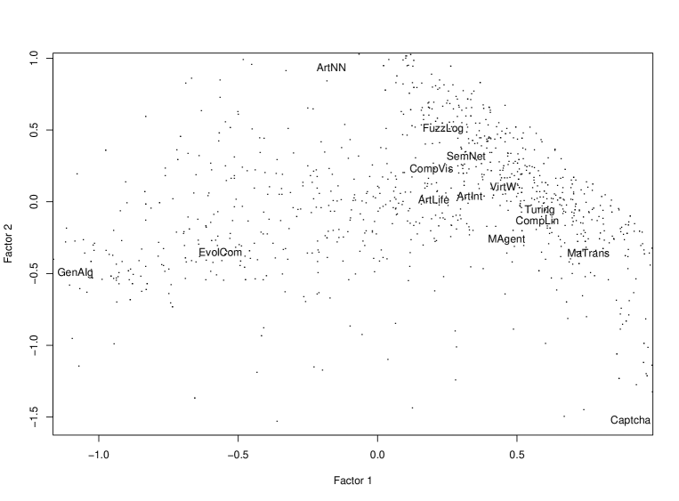
In our use of free text, we have already noted how a mapping into a Euclidean space gives us the capability to define distance in a simple and versatile way. In correspondence analysis [Murtagh 2005b], the texts we are using provide the rows, and the set of terms used comprise the column set. In the output, Euclidean factor coordinate space, each text is located as a weighted average of the set of terms; and each term is located as a weighted average of the set of texts. (This simultaneous display is sometimes termed a biplot.) So texts and terms are both mapped into the same, output coordinate space. This can be of use in understanding a text through its closest terms, or vice versa.

A commonly used methodology for studying a set of texts, or a set of parts of a text (which is what we will describe below), is to characterize each text with numbers of terms appearing in the text, for a set of terms. The $\chi^{2}$ distance is an appropriate weighted Euclidean distance for use with such data [Benzécri 1979; Murtagh 2005b]. Consider texts $i$ and $i^{\prime}$ crossed by words $j$ . Let $k_{ij}$ be the number of occurrences of word $j$ in text $i$ . Then, omitting a constant, the $\chi^{2}$ distance between texts $i$ and $i^{\prime}$ is given by $\sum_{j}1/k_{j}(k_{ij}/k_{i}-k_{i^{\prime}j}/k_{i^{\prime}})^{2}$ . The weighting term is $1/k_{j}$ . The weighted Euclidean distance is between the profile of text $i$ , viz. $k_{ij}/k_{i}$ for all $j$ , and the analogous profile of text $i^{\prime}$ . (Our discussion is to within a constant because we actually work on frequencies defined from the numbers of occurrences.)

Correspondence analysis allows us to project the space of documents (we could equally well explore the terms in the same projected space) into a Euclidean space. It maps the all-pairs $\chi^{2}$ distance into the corresponding Euclidean distance.

For a term, we use the (full rank) projections on factors resulting from correspondence analysis. As noted, this factor space is endowed with the (unweighted) Euclidean distance.

3.2 Linearity: Textual Time Series

We will also take into consideration the strongest “given” in regard to any classical text: its linearity (or total) order. A text is read from start to finish, and consequently is linearly ordered.

A text endowed with this linear order is analogous to a time series. If we use the correspondence analysis (full dimensionality) factor coordinates for each term, then the textual time series we are dealing with is seen to be a multivariate time series.

3.3 Recoding Distances

Just as the way we code our input data plays a crucial role in the resulting analysis, so also the recoding of pairwise distances can influence the analysis greatly. In Murtagh [2005a] we introduced a new distance, which we will term the “change versus no change”, CvNC, metric, and showed its benefits on a wide range of (financial, biomedical, meteorological, telecoms, chaotic, and random) time series. Motivation for using this new metric is that it greatly increases the ultrametricity of the data.

The CvNC metric is defined in the following way. Take the Euclidean distance squared, $d_{jj^{\prime}}=(x_{jr}-x_{j^{\prime}r})^{2}$ for all $1\leq j,j^{\prime}\leq m$ , where we have terms $j,j^{\prime}$ in the factor space with coordinates $1,2,\dots,r,\dots\nu$ . It will be noted below in this section how this assumption of Euclidean distance squared has worked well but is not in itself important: in principle any dissimilarity can be used.

We enforce sparseness on our given squared distance values, $\{d_{jj^{\prime}}\}$ . We do this by approximating each value $d_{jj^{\prime}}$ , in the range $\mbox{max}_{jj^{\prime}}d_{jj^{\prime}}-\mbox{min}_{jj^{\prime}}d_{jj^{\prime}}$ , by an integer in $1,2,\dots p$ . The value of $p$ must be specified. In our work we set $p=2$ . The recoding of distance squared is with reference to the mean distance squared: values less than or equal to this will be mapped to 1; and values greater than this threshold will be mapped to 2. Thus far, the recoded value, $d^{\prime}_{jj^{\prime}}$ is not necessarily a distance. With the extra requirement that $d^{\prime}_{jj^{\prime}}\longrightarrow 0$ whenever $j=j^{\prime}$ it can be shown that $d^{\prime}_{jj^{\prime}}$ is a metric [Murtagh 2005a]:

Theorem: The recoded pairwise measure, $d^{\prime}$ , defined as described above from any dissimilarity, is a distance, satisfying the properties of: symmetry, positive definiteness, and triangular inequality.

To summarize, in our coding, a small pairwise dissimilarity is mapped onto a value of 1; and a large pairwise dissimilarity is mapped onto a value of 2. Identical values are unchanged: they are mapped onto 0.

This coding can be considered as encoding pairwise relationships as “change”, i.e. 2, versus “no change”, i.e. 1, relationships. Then, based on these new distances, we use the ultrametric triangle properties to assess conformity to ultrametricity. The proportion of ultrametric triangles allows us to fingerprint our data.

For any given triplet (of terms, with pairwise CvNC distances), if the triplet is to be compatible with the ultrametric inequality, each set of three recoded distances is necessarily of one of the following patterns:

Trivial:: At least one (recoded) distance is 0, in which case we do not consider it.
Ultrametric – equilateral:: Recoded distances in the triplet are 1,1,1 or 2,2,2, defining an equilateral triangle.
Ultrametric – isosceles:: Recoded distances in the triplet are 1,2,2 in any order, defining an isosceles triangle with small base.
Non-ultrametric:: Recoded distances in the triplet are 1,1,2 in any order.

The non-ultrametric case here is seen to be an isosceles triangle with large base. We could “intervene” and change one of the values to make it ultrametric. If we change the 2-value to a 1-value, this will produce an equilateral triangle, which is ultrametric. In this case, we are approximating our three values optimally from below, and the resulting ultrametric is termed the subdominant, or maximally inferior, ultrametric. The associated stepwise algorithm for constructing a hierarchy is known as the single link hierarchical clustering algorithm. On the other hand, we could change one of the 1-values to a 2. This is not unique, since we could change either of the 1-values. The resulting hierarchy is termed the minimally superior ultrametric. The associated stepwise algorithm for constructing a hierarchy is known as the complete link hierarchical clustering algorithm. All of this is very clear from the case considered here.

The recoding into the CvNC metric is a particular example of symbolic coding. See Murtagh [2006c].

In the next section, we will show the usefulness of this CvNC metric for quantifying inherent hierarchical structure.

4 Application to Pair and Triplet Phrase Finding, and to Selecting Pertinent Terms

In this section we first describe the data set used. Next, based on the foundation of the previous section, we quantify inherent hierarchical structure in our data. This justifies going further, to harness and exploit this structure.

4.1 Data Used

We use 14 texts taken from Wikipedia (mid-2006), and coverted to straight text from HTML. Table 1 shows the numbers of words in each.

File	Theme	No.	No.	No.
		words	nouns	uniq. nouns
ArtInt	Artificial Intelligence	1624	405	231
ArtLife	Artificial Life	2095	448	275
ArtNN	Artificial Neural Network	4698	1262	389
Captcha	Captcha	1479	318	169
CompLin	Computational Linguistics	648	168	80
CompVis	Computer Vision	2396	737	311
EvolCom	Evolutionary Computation	156	58	43
FuzzLog	Fuzzy Logic	1663	399	204
GenAlg	Genetic Algorithms	2775	715	306
MaTrans	Machine Translation	1643	411	172
MAgent	Multi-agent System	493	104	67
SemNet	Semantic Network	475	96	74
Turing	Turing Test	2432	459	225
VirtW	Virtual World	583	144	79
All files			5724	1165

Table 1: Properties of texts used.

We derived 4048 unique terms (all parts of speech, including nouns) from the collection of 14 texts listed in Table 1. As noted before, we do not apply stemming. The $14\times 4048$ frequency of occurrence matrix was analyzed using correspondence analysis, which furnished an embedding of both texts and terms in a 13-dimensional (i.e., necessarily at most one less than the minimum of input row and column dimensions, viz. 14 and 4048) factor space.

Although the presence in the analysis of minor words can be important (see discussion in Murtagh [2005b]), for the concept hierarchy relationships we are primarily interested in nouns. We used therefore a part of speech tagger [Schmid 1994] to locate the nouns. The number of nouns found in the Artificial Intelligence text was 231. For each we have a 13-dimensional factor space representation, and the latter has been defined globally, using all texts in the collection studied.

For all pairs of the these 231 terms, using their 13-dimensional Euclidean characterization, we carried out the mapping into the CvNC metric.

For the Artificial Intelligence text, 36% of the triplets were equilateral; 50% of the triplets were isosceles with small base; hence 86% of the triplets respected the ultrametric inequality. Finally, 14% of the triplets were non-ultrametric.

A summary of the “fingerprinting” procedure in regard to the text’s ultrametricity, or inherent local hierarchical structure, is as follows.

1.

Define each of the relevant terms – nouns – in a Euclidean factor space.
2.

Take each triplet of terms in turn.
3.

Define the squared Euclidean distance between each successive pair of terms.
4.

Use the pairwise average of these squared distances as a threshold.
5.

If the pair of terms is of squared distance less than the threshold, then define their relationship as “no change”.
6.

If the pair of terms is of squared distance greater than or equal to the threshold, then define their relationship as “change (either up or down)”.
7.

With “no change” coded as 1, “change” coded as 2, and self-distances coded as 0, Murtagh [2005a] shows that the resulting mapping of the Cartesian product of terms $\times$ terms onto the set $d^{\prime}\in\{0,1,2\}$ defines a metric. For all terms $i,j,k$ , we therefore have $d^{\prime}_{ij}\leq d^{\prime}_{ik}+d^{\prime}_{kj}$ .
8.

For the given triplet we check if this metric is an ultrametric: For terms $i,j,k$ , we therefore seek whether $d^{\prime}_{ij}\leq\mbox{max}\{d^{\prime}_{ik},d^{\prime}_{kj}\}$ .
9.

If the triplet $i,j,k$ respects the ultrametric relation, then there are two possible cases. Firstly, the triangle formed by these terms is equilateral, which is implied whenever $d^{\prime}_{ij}=d^{\prime}_{ik}=d^{\prime}_{kj}$ . Secondly, the triangle is isosceles with small base, which is implied by two $d^{\prime}$ s being equal, and greater in value to the third.
10.

No other triangle configurations are consistent with the ultrametric relationship.
11.

Over all triplets considered, the ultrametricity index of the document is the proportion of ultrametricity-respectiving triplets.

Table 2 shows the results obtained for (i) global relationships given by all triangles (triangles were read off using the loops $i=1\dots n-2$ , $j=i+1\dots n-1$ , $k=j+1\dots n$ ); and (ii) linear relationships, using only triangles defined from successives triplets of terms in the text. Nouns were used: cf. Table 1. What we see very clearly from Table 2 is that, whether global or linear, our texts show very dominant ultrametric or hierarchical structure. Furthermore, this is, in the great majority of cases, dominated by the isosceles with small base case, relative to the “trivial” equilateral case.

These results justify going further now, in order to make use of the inherent hierarchical structure that is in our data.

Text	Total no.	No. isosc.	No. equil.	Non-UM
	triangles	triangles	triangles	triangles
Artificial Intelligence	2027795	50	36	14
	336	37	45	18
Artificial Life	3428425	52	36	12
	342	34	41	26
Artificial Neural Network	9735114	46	42	12
	914	39	49	11
Captcha	790244	54	33	12
	225	41	33	25
Computational Linguistics	82160	46	39	15
	132	47	41	12
Computer Vision	4965115	50	38	13
	578	36	40	24
Evolutionary Computation	12341	37	48	15
	52	33	54	13
Fuzzy Logic	1394204	52	33	14
	299	45	30	25
Genetic Algorithms	4728720	43	46	10
	581	37	51	12
Machine Translation	833340	49	36	15
	331	40	33	27
Multi-agent System	47905	49	42	9
	87	37	49	14
Semantic Network	64824	59	35	6
	77	35	57	8
Turing Test	1873200	50	37	13
	365	45	33	23
Virtual World	79079	58	29	13
	88	42	28	30

Table 2: Texts, and their properties as quantified, as percentages, by relative numbers of triangles. Note the percentages in columns 3, 4 and 5 sum to 100, but may deviate from this by a unit due to the rounding to the nearest integer. For each text, we show results for the global and the linear cases (see accompanying discussion for details).

4.2 Application to Concept Hierarchy Relationships

To the extent that our data satisfies, globally and throughout, the ultrametric inequality, we can adopt any of the widely used hierarchical clustering algorithms (single, complete, average linkage; minimum variance, median, centroid) to induce an identical, unique hierarchy. But when we find our data to be, say, 86% ultrametric, as is not untypically the case in practice, then we must consider carefully what our aim is. If we wished to look at each and every isosceles triangle, then in the case of the Artificial Intelligence text this means, out of a total of 2,027,795 triplets (i.e., $(231\cdot 230\cdot 229)/(2\cdot 3)$ ) we must consider 1,007,597.

What we will do instead is return to taking our text as a time series. We have 231 unique nouns in the Artificial Intelligence text. In the text, these nouns are used, in total, on 405 occasions. So our text is a time series of 405 values. For successive nouns in this textual time series, the CvNC metric has an evident meaning: we are noting semantic change versus lack of change as we read through the text.

We examine successive triplets in the textual time series. For the Artificial Intelligence text, we find 45% of the triplets to be equilateral; 37% of the triplets are isosceles; and 18% of the triplets are non-ultrametric.

The isosceles triplets point to a dominance or subsumption relationship that will be of use for us in a concept hierarchy. Say we have a triplet $x,y,z$ . Say, further, that the CvNC distance between $x$ and $y$ is 1, so therefore there is no change in progressing from use of term $x$ to use of term $y$ . However both $x$ and $y$ are at CvNC distance 2 to term $z$ , and this betokens a semantic change. So the relationship is simply represented as $((x,y)z)$ . The term $z$ dominates or subsumes $x$ and $y$ .

The following results hold.

Firstly, say that a successive triplet of values, in any order, is found as $x,y,z$ , and later in the text, again, this triplet is found in any order. Then the relationship between the three recoded distances in both cases will be identical. For a given triplet, in any order within the triplet, the relationship is unique.

Secondly, consider any other term, $w$ , such that some or all of the terms $x,y,z$ are found to have a relationship with $w$ . As an example, we meet with $y,z,x$ at one point in the text, and later we meet with $x,w,y$ . Then there is no influence by $w$ on the relationship ensuing from the $x,w,y$ triplet, vis-à-vis the relationship ensuing from the earlier $y,z,x$ triplet. We have locality of the relationship in any given triplet, from successive terms. The relationship is strictly local to the given triplet.

Among the isosceles triangles in the Artificial Intelligence text, we find the following relationships.

( computer science ) branch
( home computer ) world
( analysis systems ) formalism
( analysis systems ) reasoning
( expert system ) conclusion
( expert system ) amounts
( example networks ) reasoning
( networks learning ) reasoning
( pattern recognition ) capabilities
( control systems ) computation
( consciousness systems ) logic
( medicine computer ) commentators
( computer technology ) commentators
( application feature ) os
( application feature ) languages
( libraries systems ) specialist
( libraries systems ) programmers
( software engineering ) development
( software engineering ) practices
( programs example ) logic
( example type ) logic
( projects publications ) life
( publications bayesian ) life
( bayesian networks ) life
( cybernetics systems ) agents
( systems control ) agents
( wiki web ) website
( wiki web ) category
( algorithm implementations ) projects
( algorithm implementations ) demonstrations
( implementations research ) demonstrations
( research group ) demonstrations

However there are other isosceles triplets that are less self-evident. For this reason therefore we take all texts. For the 14 texts, we have 6439 nouns, and 1470 unique nouns. With our CvNC metric on all pairs of nouns, the complete link hierarchical clustering method gives 21 clusters in all.

While one application of the foregoing is to deriving common pairs and triplets of terms, in practice it would be better to combine all relationships into a “bigger picture”. We will address this below in section 5.

4.3 Selecting the Most Pertinent Terms

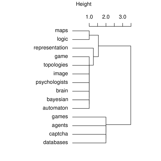
Presenting a result with around 1500 terms does not lend itself to convenient display. We ask therefore what the most useful – perhaps the most discriminating terms – are. In correspondence analysis both texts and their characterizing terms are projected into the same factor space. See Figure 1. So, from the factor coordinates, we can easily find the closest term(s) to a given text. We do this for each of the 14 texts, and find the closest terms, respectively, as follows:

     bayesian         automaton    brain          captcha
     psychologists    image        maps           logic
     topologies       databases    agents         representation
     game             games

A hierarchical clustering of these is shown in Figure 2. The Ward minimum variance method is used, as being appropriate for structuring data well (see Murtagh [1984b]) and also having an agglomerative criterion that is appropriate for the prior Euclidean embedding (viz., inertia-based in both cases). The data clustered are exactly those illustrated in the best planar projection of Figure 1: these are 14 texts in a 4048-dimensional term space. Due to centering in the dual spaces, the inherent dimensionality of both text and term spaces are: min $(14-1,4048-1)$ = 13. Based on the dual spaces, we carry out the eigen-reduction in the space of smaller original dimensionality (viz., the space of the terms, which are in a 14-dimensional space), and then subsequently project into the 4048-dimensional space.

Refer to caption — Figure 1: Correspondence analysis principal factor plane of projections of 14 texts, and 4048 terms (each represented with a dot).

Proceeding further, the 5 closest terms to any given text, based on the full inherent dimensionality of this data (viz., smaller of dimensionality of texts, and dimensionality of terms), are as follows.

Text and set of 5 closest characterizing terms:

Artificial Intelligence
bayesian intelligence consciousness brains chatterbots

Artificial Life
automaton automata biology chemical allelomimesis

Artificial Neural Networks
brain prediction forecasting aircraft epitomes

Captcha
captcha captchas robot intelligence chemistry

Computational Linguistics
psychologists logics morphology pragmatics logicians

Computer Vision
image images diagnosis dimensionality dimensions

Evolutionary Computation
maps intelligence robot biology chemistry

Fuzzy Logic
logic mapping animals brakes armies

Genetic Algorithms
topologies communications music finance representations

Machine Translation
databases chemistry database memory robot

Multi-agent System
agents agent robotics cybernetics robot

Semantic Network
representation database map namespaces robot

Turing Test
game chatterbot consciousness memory intelligence

Virtual World
games gameplay topography communication representations

5 From Hierarchical Clustering to a Hierarchy of Concepts

5.1 A Formal Approach: Displaying a Hierarchical Clustering as an Oriented Tree

We have noted in the Introduction how a hierarchical clustering may be the starting point for creating a concept hierarchy, but the two representations differ. In this section we show how we can move from an embedded set of clusters, to an oriented tree. Orientation in the latter case aims at expressing subsumption.

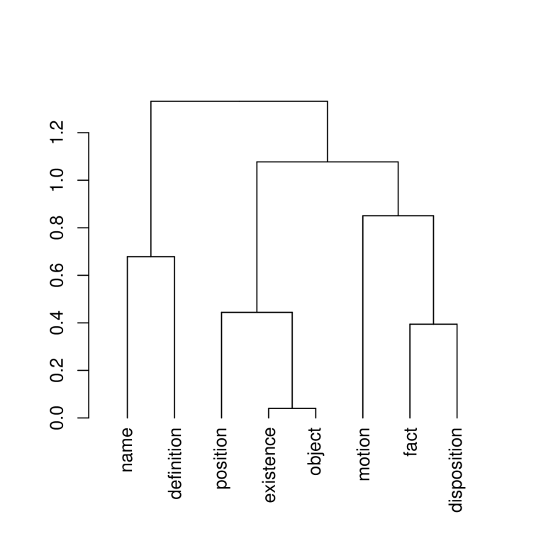
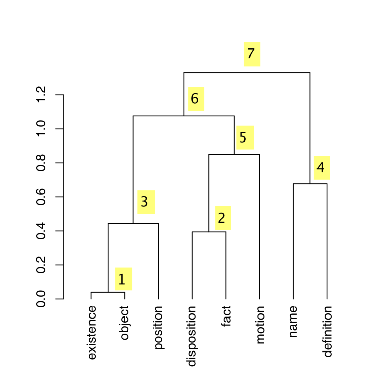
Consider the dendrogram shown in Figure 3, which represents an embedded set of clusters relating to the 8 terms. We will consider first such a strictly 2-way hierarchy, where we assume that no two agglomerations take place at precisely the same level. In the later case study, in subsection 5.4, we will consider the practical case where agglomerations take place at the same level.

Rather than the 14 texts used in section 4, to clarify the presentation in this section we will take just one text.

We took Aristotle’s Categories, which consisted of 14,483 individual words. We broke the text into 24 files, in order to base the textual analysis on the sequential properties of the argument developed. In these 24 files there were 1269 unique words. We selected 66 nouns of particular interest. A sample (with frequencies of occurrence): man (104), contrary (72), same (71), subject (60), substance (58), … No stemming or other preprocessing was applied. For the hierarchical clustering, we further restricted the set of nouns to just 8. (These will be seen in the figures to be discussed below.) The data array was doubled [Murtagh 2005b] to produce an $8\times 48$ array, which with removing 0-valued text segments (since, in one text segment, none of our selected 8 nouns appeared) gave an $8\times 46$ array, thereby enforcing equal weighting of (equal masses for) the nouns used. The spaces of the 8 nouns, and of the 23 text segments (together with the complements of the 23 text segments, on account of the data doubling) are characterized at the start of the correspondence analysis in terms of their frequencies of occurrence, on which the $\chi^{2}$ metric is used. The correspondence analysis then “euclideanizes” both nouns and text segments. We used a 7-dimensional (corresponding to the number of non-zero eigenvalues found) Euclidean embedding, furnished by the projections onto the factors. A hierarchical clustering of the 8 nouns, characterized by their 7-dimensional (Euclidean) factor projections, was carried out: Figure 3. The Ward minimum variance agglomerative criterion was used, with equal weighting of the 8 nouns.

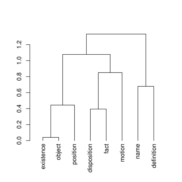
Figure 4 shows a canonical representation of the dendrogram in Figure 3. Both trees are isomorphic to one another. Figure 4 is shown such that the sequence of agglomerations is portrayed from left to right (and of course from bottom to top). We say that Figure 4 is a canonical representation of the dendrogram, implying that Figure 3 is not in canonical form. In Figure 5, the canonical representation has its non-terminal nodes labeled.

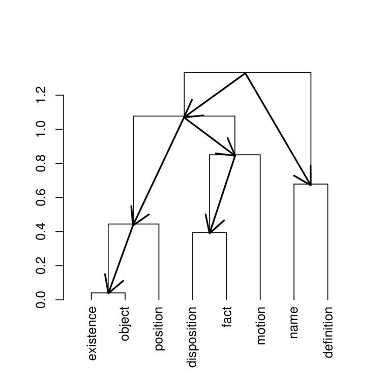
Next, Figure 6 shows a superimposed oriented binary rooted tree, on $n-1$ nodes, which is isomorphic to the dendrogram on $n$ terminal nodes. This oriented binary tree is an inorder traversal of the dendrogram. Sibson’s [1973] “packed representation” of a dendrogram uses just such an oriented binary rooted tree, in order to define a permutation representation of the dendrogram. From our example, the packed representation permutation can be read off as: $(13625748)$ : for any terminal node indexed by $i$ , with the exception of the rightmost which will always be $n$ , define $p(i)$ as the rank at which the terminal node is first united with some terminal node to its right. Discussion of combinatorial properties of dendrograms, as related to such oriented binary rooted trees, and associated down-up and up-down permutations, can be found in Murtagh [1984a].

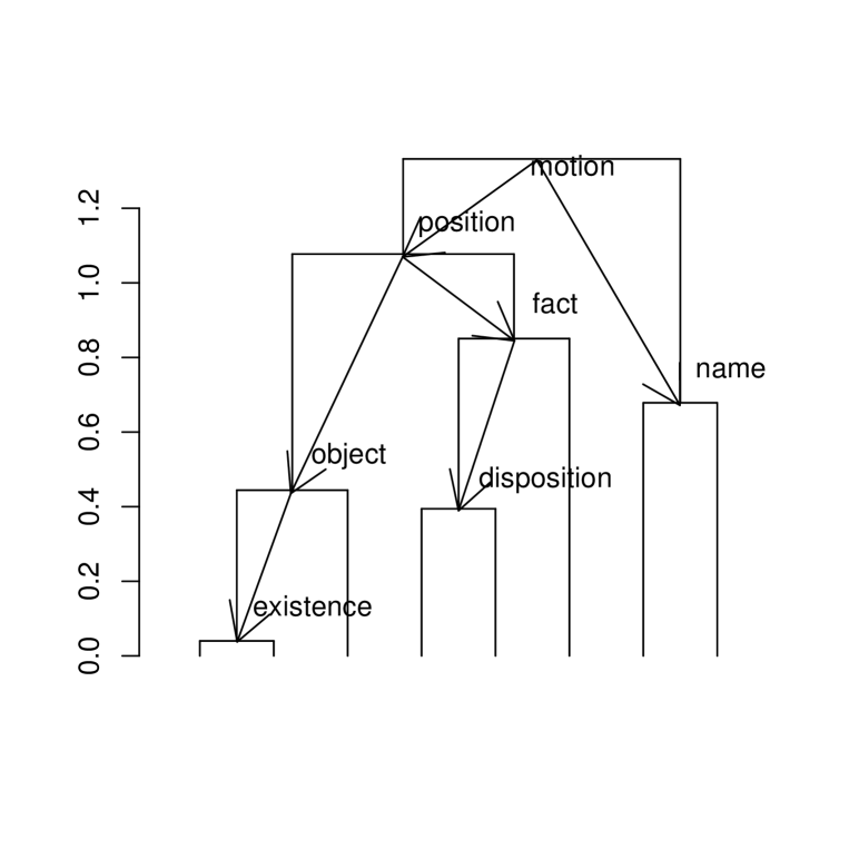
Finally, in Figure 7, we “promote” terminal node labels to the nodes of the oriented tree. We will use exactly the procedure used above for defining a permutation representation of the oriented tree. First the left terminal label is promoted to its non-terminal node. Next, the right terminal label is promoted as far up the tree as is necessary in order to find an unlabeled non-terminal node. This procedure is carried out for all non-terminal labels, working in sequence from left to right (i.e., consistent with our canonical representation of the dendrogram). The rightmost label is not shown: it is at an arbitrary location in the upper right hand side, with a tree arc oriented towards the top non-terminal node of the dendrogram, now labeled as “motion”.

In this section, we have specified a consistent procedure for labeling the nodes of an oriented tree, starting from the labels associated with the terminal nodes of a dendrogram. We start therefore with embedded clusters, and end up with terms and directed links between these terms. There is some non-uniqueness: any two labels associated with terminal nodes that are left and right child nodes of one non-terminal node can be interchanged. This clearly leads to a different label promotion outcome.

Our promotion procedure was motivated by the permutation representation of an oriented binary tree, as described above. Here too we do not claim uniqueness of permutation representation. But we do claim optimality in the sense of parsimony, and well-definedness.

In the case of a multiway tree with very few distinct levels, the promotion procedure becomes very simple, but continues to be non-unique.

5.2 A New Approach to Deriving a Concept Hierarchy from a Dendrogram

In the previous subsection, we discussed an algorithm which takes a hierarchical clustering, and hence a dendrogram, into an inorder tree traversal, and hence a permutation of the set of terms used. The formal procedure discussed in the previous subsection suffers from non-uniqueness: alternative permutations could be defined. This leads us to question the relationship of subsumption (or direction in the oriented tree). In this section we will develop another approach which is even more closely associated with the data that we are analyzing.

We have already seen that triangle properties between triplets of points, or data objects, are fundamental to ultrametricity and hence to tree representation. A dendrogram, representing a hierarchical clustering, allows us to read off, for all triplets of points, either (i) isosceles triangles, with small base, or (ii) equilateral triangles, and (iii) no other triangle configuration. The reason for the last condition is simply that non-isosceles, or isosceles with large base, triangles are incompatible with the ultrametric, or tree, metric.

We will leave aside for the present the equilateral triangle case. Firstly, it implies that all 3 points are ex aequo in the same cluster. Secondly, therefore we will treat them altogether as a concept cluster. Thirdly, the equilateral case does not arise in the example we will now explore.

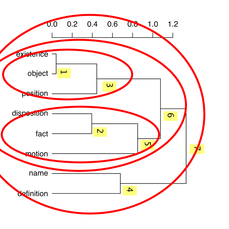
In Figure 8, cluster number 3 indicates the following isosceles triangle with small base: ((existence, object) position). Our notation is: ((x, y) z), such that triplet x, y, z has small base x, y, and the side lengths x, z and y, z are equal. This is necessarily implied by relationships represented in Figure 8. So, motivated by this triangle view of the cluster number 3 part of the dendrogram we will promote “position” to the cluster number 3 node.

Similarly we will promote “motion” to the cluster number 5 node.

Note the consistency of our perspective on the cluster number 3 and 5 nodes relative to how the associated terms here form an isosceles triangle with small base.

We will straight away generalize this definition. In any case of a node in the form of nodes 3 or 5, where we have a 2-term left subtree, and a 1-term right subtree, where left and right are necessarily labeled in this way given the canonical representation of the dendrogram, then: the left subtree is dominated by the right subtree.

We will next look at cluster number 6 (remaining with Figure 8). As always for such trees, the node corresponding to this cluster has two subtrees, one to the left (here: 3) and one to the right (here: 5). Since our dendrogram is in canonical form, any such node has a subtree with smallest non-terminal node level to the left; and the subtree which was more recently formed in the sequence of agglomerations to the right. Based on either or both of these criteria which serve to define what are the left and right subtrees we define the ordering relationship: the left subtree is dominated by the right subtree.

FIGURE NOT AVAILABLE: SEE PDF VERSION OF PAPER AT www.cs.rhul.ac.uk/home/fionn/papers/auto_onto.pdf

Figure 9: Concept relationships, ordered by dominance, derived from the dendrogram in Figure 8.

Figure 9 summarizes the concept relations that we can derive in a similar way from any dendrogram.

5.3 Demonstrator

Figure 10 indicates how the concept relations, shown in Figure 9, are to be used.

Firstly the term set is summarized, using our selection of terms. Scaling to large data sets is addressed in this way.

Secondly, in our interactive implementation (web address:
thames.cs.rhul.ac.uk/ $\sim$ dimitri/textmap), we allow the terms shown to continually move in a limited way, to get around the occlusion problem, and we also allow magnification of the display area for this same reason.

Thirdly, terms other than those shown are highlighted when a cursor is passed over them.

Next, double clicking on any term gives a ranked list of text segment names, ordered by frequency of occurrence by this term. Clicking on the text segment gives the actual text at the bottom of the display area.

5.4 Application with Ex Aequo Terms and Clusters

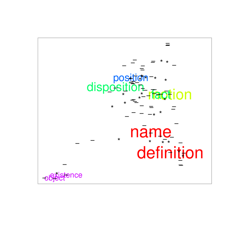
We proceed now to a third case study of this work, where we have a multiway hieararchy (and not a binary hierarchy) from the start. We require a frequency of occurrence matrix which crosses the terms of interest with parts of a free text document. For the latter we could well take documentary segments like paragraphs. O’Neill [2006] is a 660-word discussion of ubiquitous computing from the perspective of human computing interaction. With this short document we used individual lines (as proxies for the sequence of sentences) as the component parts of the document. There were 65 lines. This facilitates retrieval of a small segment of such a single document. We chose this text to work with because it is a very small text (a single text compared to the data used in section 4, and a far smaller text compared to that used in section 5).

Based on a list of nouns and substantives furnished by the part-of-speech tagger (Schmid, 1994), we focused on the following 30 nouns:

support = $\{$ “agents”, “algorithms”, “aspects”, “attempts”, “behaviours”, “concepts”, “criteria”, “disciplines”, “engineers”, “factors”, “goals”, “interactions”, “kinds”, “meanings”, “methods”, “models”, “notions”, “others”, “parts”, “people”, “perceptions”, “perspectives”, “principles”, “systems”, “techniques”, “terms”, “theories”, “tools”, “trusts”, “users” $\}$ .

This set of 30 terms was used to characterize through presence/absence the 65 successive lines of text, leading to correspondence analysis of the $65\times 30$ presence/absence matrix. This yielded then the definition of the 30 terms in a factor space. In principle the rank of this space (taking account of the trivial first factor in correspondence analysis, relating to the centering of the cloud of points) is min( $65-1,30-1$ ). However, given the existence of zero-valued rows and/or columns, the actual rank was 25. Therefore the full rank projection of the terms into the factor space gave rise to 25-dimensional vectors for each term, and these vectors are endowed with the Euclidean metric.

Define this set of 30 terms as the support of the document. Based on their occurrences in the document, we generated the following reduced version of the document, defined on this support, which consists of the following ordered set of 52 terms:

Reduced document = “goals” “techniques” “goals” “disciplines” “meanings” “terms” “others” “systems” “attempts” “parts” “trusts” “trusts” “people” “concepts” “agents” “notions” “systems” “people” “kinds” “behaviours” “people” “factors” “behaviours” “perspectives” “goals” “perspectives” “principles” “aspects” “engineers” “tools” “goals” “perspectives” “methods” “techniques” “criteria” “criteria” “perspectives” “methods” “techniques” “principles” “concepts” “models” “theories” “goals” “tools” “techniques” “systems” “interactions” “interactions” “users” “perceptions” “algorithms”

This reduced document is just the “time series” of the nouns of interest to us, as they are used in traversing the document from start to finish. Each noun in the sequence of 52 nouns is represented by its 25-dimensional factor space vector.

Out of 43 unique triplets, with self-distances removed, we found 31 to respect the ultrametric inequality, i.e. 72%. Our measure of ultrametricity of this document, based on the support used, was thus 0.72.

For a concept hierarchy we need an overall fit to the data. Using the Euclidean space perspective on the data, furnished by correspondence analysis, we can easily define a terms $\times$ terms distance matrix; and then hierarchically cluster that. Consistent with our analysis we recode all these distances, using the CvNC mapping onto $\{1,2\}$ for unique pairs of terms.

Now approximating a global ultrametric from below, achieved by the single linkage agglomerative hierarchical clustering method (and this best fit from below, termed the subdominant or maximal inferior ultrametric, is optimal), and an approximation from above, achieved by the complete linkage agglomerative hierarchical clustering method (and this best fit from above, termed a minimal superior ultrametric, is non-unique and hence is one of a number of best fits from above), will be identical if the data is fully ultrametric-embeddable. If we had an ultrametricity coefficient equal to 1 – we found it to be 0.72 for this data – then it would not matter what agglomerative hierarchical clustering algorithm (among the usual Lance-Williams methods) that we select.

In fact, we found, with an ultrametricity coefficient equal to 0.72, that the single and complete linkage methods gave an identical result. This result is shown in Figure 11.

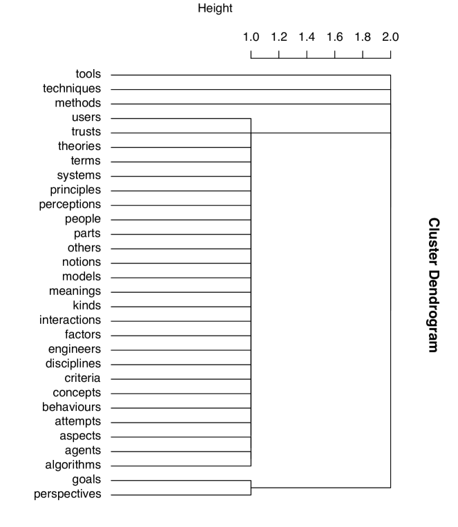
A convenient label promotion procedure to apply here is first to re-represent the terminal labels from left to right as: $\{$ “users”, “trusts”, $\dots$ , “agents”, “algorithms” $\}$ ; $\{$ “goals”, “perspectives” $\}$ ; $\{$ “tools” $\}$ ; $\{$ “techniques” $\}$ ; and $\{$ “methods” $\}$ . This is the canonical form, with ordering of left and right subtrees now extended to all subtrees.

Next, we must in fairness take the nodes at level 2 as being ex aequo, $\{$ “tools” $\}$ ; $\{$ “techniques” $\}$ ; and $\{$ “methods” $\}$ . Similarly at level 1, we also have two clusters that are ex aequo: $\{$ “users”, “trusts”, $\dots$ , “agents”, “algorithms” $\}$ ; and $\{$ “goals”, “perspectives” $\}$ .

FIGURE NOT AVAILABLE: SEE PDF VERSION OF PAPER AT www.cs.rhul.ac.uk/home/fionn/papers/auto_onto.pdf

Figure 12: Concept hierarchy derived, using our methodology, from Figure 11. See accompanying discussion for details.

Figure 12 shows our resulting scheme where level 1 clusters dominate level 2 clusters.

This provides our ontology. The granularity of this one document is, as mentioned above, line-based, and there are 65 lines in all. Hence retrieval of one or more of these document snippets is supported, and the ontology is based on a 30-noun document support.

6 Conclusions

Having first appraised text collections in terms of their local hierarchical structure, we then proceeded in this work to show how this new methodology could be employed for a wide range of tasks that include:

•

finding salient pairs and triplets of terms, which are not necessarily in sequence;
•

permitting us to consider any given text as a whole with all pairwise relationships between terms, or alternatively as a time series with relationships restricted to terms that are successive in sequence;
•

passing seamlessly from the exploration of local hierarchical structure to global hierarchical structure;
•

especially when global hierarchical structure is manifest, being able to use any of a wide range of agglomerative clustering criteria to furnish the same resultant hierarchy;
•

determining a hierarchy of concepts from the embedded, partially ordered subsets provided by a hierarchical clustering;
•

obtaining unique results when given a 2-way hierarchical clustering tree, and then readily generalizing this to the practical case of multiway trees;
•

exemplifying an efficient and an effective textual data processing pipeline; and
•

through the measurement of local hierarchical structure, having available an approach to validating the appropriateness of any data for this data analysis pipeline.

By analysis of text through local hierarchical relationships between terms we determine extensive internal textual structure, without being stifled by the more traditional approach of fitting some global structure, such as a hierarchy, to the text. A (local) hierarchical structure is a powerful one: it includes peer as well as subsumption types of relationships.

We stress that we can find very pronounced hierarchical structures of this sort if we encode the text is novel ways. An example is to start with a Euclidean spatial embedding of the terms and documents (or segments of a document), which is quite traditional; and then look at interrelationships between terms using “relatively close/similar” versus “relatively distant/new” (and this alone can be shown to have metric properties). Another example of an encoding-related strategy is not to take into consideration all interrelationships between terms, but only between successive terms, and thereby view the text as a particular type of time series. User interactivity with the system is to select the terms of interest (people’s personal names, industrial product names, location or venue names, etc.). The interrelationships between these terms are then explored through their local hierarchical links.

Our general application targeted is, as stated in Murtagh et al. [2003], to have readily available a self-description of data, as a basis for visually-based interactive and responsive querying of, retrieval from, and navigation of data collections.

Acknowledgement

This work was carried out in the context of the European Union Sixth Framework project, “WS-Talk, Web services communicating in the language of their community”, 2004–2006. Pedro Contreras and Dimitri Zervas contributed to this work. The Textmap demonstrator was developed by Dimitri Zervas.

References

: ABOU ASSALI, A. and ZANGHI, H. 2006. Automated metadata hierarchy derivation. In Proc. IEEE ICTTA06 (Damascus, Syria).
: AHMAD, K. and GILLAM, L. (2005). Automatic ontology extraction from unstructured texts. In ODBASE 2005.
: BENZÉCRI, J.P. (1979). L’Analyse des Données, Tome I Taxinomie, Tome II Correspondances, 2nd ed. (Dunod, Paris).
: CHUANG SHUI-LUNG and CHIEN LEE-FENG (2005). Taxonomy generation for text segments: a practical web-based approach, ACM Transactions on Information Systems. 23, 363–396.
: DE SOETE, G. (1986). A least squares algorithm for fitting an ultrametric tree to a dissimilarity matrix. Pattern Recognition Letters, 2, 133–137.
: DENNY, M. (2004). Ontology tools survey, Revisited, at
http://www.xml.com/pub/a/2004/07/14/onto.html, July 2004.
: DOYLE, L.B. (1961). Semantic road maps for literature searches. Journal of the ACM. 8, 553–578.
: GANESAN, P., GARCIA-MOLINA, H. and WIDOM, J. (2003). Exploiting hierarchical domain structure to compute similarity. ACM Transactions on Information Systems. 21, 64–93.
: GÓMEZ-PÉREZ, A., FERNÁNDEZ-LÓPEZ, M. and CORCHO, O. (2004). Ontological Engineering (with Examples from the Areas of Knowledge Management, e-Commerce and the Semantic Web) (Springer, Berlin).
: GRUBER, T. (2001). What is an ontology?, http://www-ksl.stanford.edu/kst/what-is-an-ontology.html, Sept. 2001.
: JANOWITZ, M.F. (2005). Cluster analysis based on abstract posets, preprint. Also presentation, ENST de Bretagne, 30 Oct. 2004; DIMACS, 9 Mar. 2005; and SFC, 31 May 2005.
: MAEDCHE, A. (2006). Ontology Learning for the Semantic Web (Kluwer, Dordrecht).
: MURTAGH, F. (1984a). Counting dendrograms: a survey. Discrete Applied Mathematics, 7, 191–199.
: MURTAGH, F. (1984b). Structures of hierarchic clusterings: implications for information retrieval and for multivariate data analysis. Information Processing and Management, 20, 611–617.
: MURTAGH, F. (2004). On ultrametricity, data coding, and computation, Journal of Classification, 21, 167–184.
: MURTAGH, F. (2005a). Identifying the ultrametricity of time series, European Physical Journal B, 43, 573–579.
: MURTAGH, F. (2005b). Correspondence Analysis and Data Coding with R and Java (Chapman & Hall/CRC).
: MURTAGH, F. (2006a). Ultrametricity in data: identifying and exploiting local and global hierarchical structure, arXiv:math.ST/0605555v1 19 May 2006.
: MURTAGH, F. (2006b). The Haar wavelet transform of a dendrogram,
arXiv:cs.IR/0608107v1 28 Aug 2006, forthcoming in Journal of Classification.
: MURTAGH, F. (2006c). Symbolic dynamics in text: application to automated construction of concept hierarchies, Festschrift for Edwin Diday, in press. Available at: www.cs.rhul.ac.uk/home/fionn/papers
: MURTAGH. F. (2006d). Visual user interfaces, interactive maps, references, theses, http://astro.u-strasbg.fr/ $\sim$ fmurtagh/inform
: MURTAGH, F., TASKAYA, T., CONTRERAS, P., MOTHE, J. and ENGLMEIER, K. (2003). Interactive visual user interfaces: a survey, Artificial Intelligence Review, 19, 263–283.
: O’NEILL, E. (2006). Understanding ubiquitous computing: a view from HCI, in Discussion following R. Milner, Ubiquitous computing: how will we understand it?, Computer Journal, 49, 390–399.
: SCHMID, H. (1994). Probabilistic part-of-speech tagging using decision trees. In Proc. Intl. Conf. New Methods in Language Processing (see TreeTagger site).
: TreeTagger, www.ims.uni-stuttgart.de/projekte/corplex/TreeTagger/ DecisionTreeTagger.html
: SIBSON, R. (1973). SLINK: an optimally efficient algorithm for the single-link cluster method, Computer Journal, 16, 30–34.
: WACHE, H., VÖGELE, T., VISSER, U., STUCKENSCHMIDT, H., SCHUSTER, G., NEUMANN, H. and HÜBNER, S. (2001). Ontology-based integration of information – a survey of existing approaches. In Proceedings of the IJCAI-01 Workshop: Ontologies and Information Sharing.