Characterization of Rate Region in Interference Channels with Constrained Power

Abstract

In this paper, an $n$-user Gaussian interference channel, where the power of the transmitters are subject to some upper-bounds is studied. We obtain a closed-form expression for the rate region of such a channel based on the Perron-Frobenius theorem. While the boundary of the rate region for the case of unconstrained power is a well-established result, this is the first result for the case of constrained power. We extend this result to the time-varying channels and obtain a closed-form solution for the rate region of such channels.

I Introduction

Channel sharing is known as an efficient scheme to increase the spectral efficiency of the wireless systems. While such a scheme increases the capacity and the coverage area of systems, it suffers from the interference among the concurrent links (co-channel interference). Consequently, the signal-to-interference-plus-noise-ratio (SINR) of the links are upper-bounded, even if there is no constraint on the transmit powers.

There have been some efforts to evaluate the maximum achievable SINR in the interference channels. In [1], the maximum achievable SINR of a system with no constraint on the power is expressed in terms of the Perron-Frobenius eigenvalue of a non-negative matrix and this result is utilized to develop an SINR-balancing scheme for satellite networks. This formulation for the maximum achievable SINR is deployed in many other wireless communication applications such as [2, 3, 4, 5] afterwards.

Recently, the rate region of interference channels and its properties has been investigated in the literature. In [6], it is shown that the capacity region when the power is unbounded is convex. The capacity region in [6] is defined as the set of feasible processing gains while for a constant bandwidth, the processing gain is inversely proportional to the rate. In [7], some topological properties of the capacity region (with the aforementioned definition) of CDMA systems are investigated for the cases when there are constraints on the power of individual users and when there is no constraint on the power. The authors in [7] show that the boundary of the capacity region with one user’s power fixed and the rest unbounded is a shift of the boundary of some capacity region with modified parameters, but unlimited power. However, this result is not in a closed form and can not be extended for the other forms of power constraints.

It is shown that the feasible SINR region is not convex, in general [8, 9, 10]. In [11], it is shown that in the case of unlimited power, the feasible SINR region is log-convex. The authors in [6] also consider a CDMA system without power constraints, and show that the feasible inverse-SINR region is a convex set. In [8], it is proved that the feasible quality of service (QoS) region is a convex set, if the SINR is a log-convex function of the corresponding QoS parameter. Reference [12] shows that under a total power constraint, the infeasible SINR region is not convex.

In this paper, we extend the result on the maximum achievable SINR in [1] to the systems with certain constraints on the power of transmitters. This result which is based on Perron-Frobenius theorem, yields a closed-form solution for the rate region of the systems with constrains on the power. The extendable structure of constraints enables us to use the proposed derivation for the maximum achievable SINR in many practical systems. This result is extended to a time-varying system, where the channel gain is selected from a limited-cardinality set, and the average power of users are subject to some upper-bounds.

Notation: All boldface letters indicate column vectors (lower case) or matrices (upper case). $x_{ij}$ and $\mathbf{x}_{i}$ represent the entry $(i,j)$ and column $i$ of the matrix $\mathbf{X}$, respectively. A matrix $\mathbf{X}_{n\times m}$ is called non-negative if $x_{ij}\geq 0,\ \forall i,j$, and denoted by $\mathbf{X}\geq\mathbf{0}$. Also, we have

$$\mathbf{X}\geq\mathbf{Y}\Longleftrightarrow\mathbf{X}-\mathbf{Y}\geq\mathbf{0},$$

where $\mathbf{X},\mathbf{Y}$ and $\mathbf{0}$ are non-negative matrices of compatible dimensions [13]. $\det(\mathbf{X})$, $\mathrm{Tr}(\mathbf{X})$, $\mathbf{X}^{\prime}$, and $|\mathbf{X}|$ denote the determinant, the trace, the transpose, and the norm of the matrix $\mathbf{X}$, respectively. $\mathbf{I}$ is an identity matrix with compatible size. $\otimes$ represents the Kronecker product operator. $\textrm{diag}(\mathbf{x})$ is a diagonal matrix whose main diagonal is $\mathbf{x}$. We define the reciprocal of polynomial $\mathrm{q}(x)$ of degree $m$ as $x^{m}\mathrm{q}(\frac{1}{x})$. $\psi(\mathbf{X},\mathbf{y},\mathcal{S})$ is a matrix defined as a function of three parameters, which are respectively a matrix, a vector and a set of indices,

$$\psi(\mathbf{X},\mathbf{y},\mathcal{S})=\mathbf{Z}=[\mathbf{z}_{j}],\quad\mathbf{z}_{j}=\left\{\begin{array}[]{ll}\mathbf{x}_{j}+\mathbf{y}&j\in\mathcal{S}\\ \mathbf{x}_{j}&\mathrm{otherwise}\end{array}\right.$$

II Problem Formulation

An interference channel, including $n$ links (users), is represented by the gain matrix $\mathbf{G}=[g_{ij}]_{n\times n}$ where $g_{ij}$ is the attenuation of the power from transmitter $j$ to receiver $i$. This attenuation can be the result of fading, shadowing, or the processing gain of the CDMA system. A white Gaussian noise with zero mean and variance $\sigma_{i}^{2}$ is added to each signal at the receiver $i$ terminal. In many applications, the QoS of the system is measured by an increasing function of SINR. In an interference channel, SINR of each user, denoted by $\gamma_{i}$, is

$$\gamma_{i}=\dfrac{g_{ii}p_{i}}{\sigma_{i}^{2}+\displaystyle\sum_{\begin{subarray}{c}j=1\\ j\neq i\end{subarray}}^{n}{g_{ij}p_{j}}},\quad\forall i\in\{1,\ldots,n\},$$

where $p_{i}$ is the power of transmitter $i$. In addition, in practice, the power vector $\mathbf{p}$ is subject to a set of constraints. The main goal is to find the maximum SINR which can be obtained by all users in the presence of such constraints. To this end, we solve the following optimization problem

$$\max\gamma$$ (1)

$$\mathrm{s.t.}\quad \gamma_{i}\geq\mu_{i}\gamma$$ (2)

$$\mathbf{p}\geq\mathbf{0}$$ (3)

$$\displaystyle\sum_{i\in\Omega}{p_{i}}\leq\overline{p}_{\Omega},$$ (4)

where $\Omega\subseteq\{1,\ldots,n\}$ with $k$ elements and $\boldsymbol{\mu}$ is a given vector with $\mu_{i}\geq 0$ and $|\boldsymbol{\mu}|=1$. As we will see, the solution can be easily extended for the case of multiple power constraints of the form $\displaystyle\sum_{i\in\Omega}{p_{i}}\leq\overline{p}_{\Omega}$ for different $\Omega\subseteq\{1,\ldots n\}$. $\boldsymbol{\mu}$ provides the flexibility of satisfying different rate services for different users. According to Fig. 1, the solution of (1) yields the maximum achievable SINR in the direction of vector $\boldsymbol{\mu}$. Although the numerical solution of this problem is already obtained through geometric programming [14], [15], we propose a different approach which leads to a closed-form result.

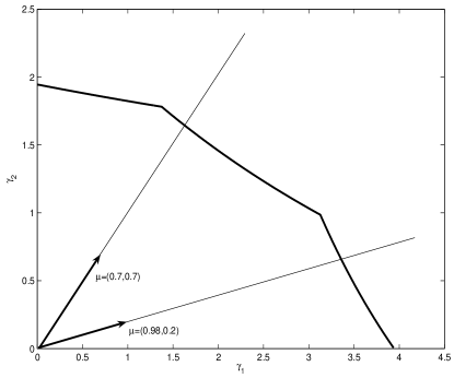
Figure 1: The boundary of SINR Region for an interference channel with $2$ users

By defining the normalized gain matrix $\mathbf{A}$ as

$$\mathbf{A}=[a_{ij}]_{n\times n},\quad a_{ij}=\left\{\begin{array}[]{ll}\dfrac{g_{ij}}{g_{ii}}&i\neq j\\ 0&i=j\end{array}\right.$$

the constraint (2) is rewritten as

$$\dfrac{p_{i}}{\eta_{i}+\displaystyle\sum_{j=1}^{n}{\mu_{i}a_{ij}p_{j}}}\geq\gamma,\quad\forall i\in\{1,\ldots,n\},$$ (5)

where

$$\eta_{i}=\dfrac{\mu_{i}\sigma_{i}^{2}}{g_{ii}},\quad\boldsymbol{\eta}=[\eta_{i}]_{n\times 1}.$$ (6)

Since we are interested in maximizing the minimum SINR, if SINR of one user is more than that of the others, it can reduce its power to other users’ advantage, and finally the minimum SINR is improved. Therefore, equality holds in (5) as

$$\dfrac{p_{i}}{\eta_{i}+\displaystyle\sum_{j=1}^{n}{\mu_{i}a_{ij}p_{j}}}=\gamma,\quad\forall i\in\{1,\ldots,n\}.$$

After reformulating the problem in a matrix form we will have

$$\big{(}\dfrac{1}{\gamma}\mathbf{I}-\mathrm{diag}{(\boldsymbol{\mu})}\mathbf{A}\big{)}\mathbf{p}=\boldsymbol{\eta}.$$ (7)

The objective is to find the maximum $\gamma$ while the system of linear equations in (7) yields a power satisfying the constraints on the power vector (3), (4).

When there is no constraint on the power vector (rather than trivial constraint of $\mathbf{p}\geq\mathbf{0}$), the maximum achievable SINR, $\gamma^{*}$, is characterized based on the Perron-Frobenius theorem as

$$\gamma^{*}=\dfrac{1}{\lambda^{*}{\big{(}\mathrm{diag}{(\boldsymbol{\mu})}\mathbf{A}\big{)}}}.$$ (8)

where $\lambda^{*}$ is the Perron-Frobenius eigenvalue of the associated matrix [13]. This result was deployed in the communication systems for SINR-balancing ($\mu_{1}=\mu_{2}=\ldots=\mu_{n}$) in [1] for the first time.

We find the maximum achievable SINR, considering certain upper-bounds on the power of transmitters in the following sections.

III SINR Region Characterization

We define $\mathbf{F}$ as

$$\mathbf{F}=\mathbf{I}-\gamma\mathrm{diag}{(\boldsymbol{\mu})}\mathbf{A}.$$ (9)

Then, the system of linear equations in (7) is reformulated as

$$\mathbf{Fp}=\gamma\boldsymbol{\eta},$$ (10)

where $\boldsymbol{\eta}$ is defined in (6). According to the Cramer’s rule, the solution to (10) is obtained by

$$p_{i}=\dfrac{\det(\mathbf{H}^{(i)})}{\det(\mathbf{F})},$$

where

$$\mathbf{H}^{(i)}=[\mathbf{{h}}^{(i)}_{j}]_{n\times n},\quad\mathbf{{h}}^{(i)}_{j}=\left\{\begin{array}[]{ll}\gamma\boldsymbol{\eta}&j=i\\ \mathbf{{f}}_{j}&j\neq i\end{array}\right..$$ (11)

Defining $\mathrm{h}^{(i)}(\gamma)=\det(\mathbf{H}^{(i)})\quad\mathrm{and}\quad\mathrm{f}(\gamma)=\det(\mathbf{F}),$ we have

$$p_{i}=\dfrac{\mathrm{h}^{(i)}(\gamma)}{\mathrm{f}(\gamma)}.$$

Therefore, the constraint in (4) can be written as

$$\dfrac{\displaystyle\sum_{i\in\Omega}{\mathrm{h}^{(i)}(\gamma)}}{\mathrm{f}(\gamma)}\leq\overline{p}_{\Omega}.$$ (12)

Defining

$$\mathrm{u}_{\Omega}(\gamma)=\overline{p}_{\Omega}\mathrm{f}(\gamma)-\displaystyle\sum_{i\in\Omega}{\mathrm{h}^{(i)}(\gamma)},$$

the inequality (12) is equivalent to

$$\dfrac{\mathrm{u}_{\Omega}(\gamma)}{\mathrm{f}(\gamma)}\geq 0.$$ (13)

We desire to find the largest possible interval where both the numerator and the denominator have the same sign. It can be shown that this interval is connected and adjacent to zero. Apparently, $\mathrm{u}_{\Omega}(0)>0,\quad\mathrm{and}\quad\mathrm{f}(0)>0.$ Consequently,

$$\exists\quad\epsilon>0\quad:\quad\mathrm{f}(\epsilon)>0\quad\mathrm{and}\quad\mathrm{u}_{\Omega}(\epsilon)>0.$$

Therefore, both the numerator and the denominator are positive in the positive neighborhood of zero. For satisfying (13), we have to find the smallest positive real simple root of the numerator and the denominator, $r(\mathrm{u}_{\Omega})$ and $r(\mathrm{f})$, and take the minimum of the two as

$$\hat{\gamma}=\min{\{r(\mathrm{f}),r(\mathrm{u}_{\Omega})\}}.$$ (14)

For the sake of simplicity, without loss of generality, we assume that $\Omega=\{1,\ldots,k\}$, $k\leq n$, i.e., the first $k$ users are subject to the total power constraint. For the numerator we have

$$\mathrm{u}_{\Omega}(\gamma) =\overline{p}_{\Omega}\det{(\mathbf{F})}-\displaystyle\sum_{i=1}^{k}{\det{(\mathbf{H}^{(i)})}}$$

$$=\overline{p}_{\Omega}\big{(}\det{(\mathbf{F})}-\displaystyle\sum_{i=1}^{k}{\det{(\mathbf{\hat{H}}^{(i)})}}\big{)},$$ (15)

where $\mathbf{\hat{H}}^{(i)}$ is defined as

$$\mathbf{\hat{H}}^{(i)}=[\mathbf{\hat{h}}^{(i)}_{j}]_{n\times n},\quad\mathbf{\hat{h}}^{(i)}_{j}=\left\{\begin{array}[]{ll}\dfrac{\gamma\boldsymbol{\eta}}{\overline{p}_{\Omega}}&j=i\\ \mathbf{{f}}_{j}&j\neq i\end{array}\right..$$

Lemma 1

If square matrices $\mathbf{X}$ and $\mathbf{Y}$ differ only in column $i$, i.e.,

$$\left\{\begin{array}[]{l}\mathbf{x}_{j}\neq\mathbf{y}_{j}\quad j=i\\ \mathbf{x}_{j}=\mathbf{y}_{j}\quad j\neq i\end{array}\right.,$$

then

$$\det\big{(}\mathbf{X})+\det(\mathbf{Y}\big{)} =\det{\big{(}\psi(\mathbf{X},\mathbf{y}_{i},\{i\})\big{)}}$$

$$=\det{\big{(}\psi(\mathbf{Y},\mathbf{x}_{i},\{i\})\big{)}}.$$

Equation (15) is rewritten as

$$\mathrm{u}_{\Omega}(\gamma)=\overline{p}_{\Omega}\big{(}\det{(\mathbf{F})}-\det(\mathbf{\hat{H}}^{(1)})-\displaystyle\sum_{i=2}^{k}{\det{(\mathbf{\hat{H}}^{(i)})}}\big{)}.$$ (16)

Since $\mathbf{F}$ and $\mathbf{\hat{H}}^{(1)}$ are the same except for the first column, using Lemma 1 , we will have

$$\det{(\mathbf{F})}-\det(\mathbf{\hat{H}}^{(1)})=\det{\big{(}\psi(\mathbf{F},-\dfrac{\gamma\boldsymbol{\eta}}{\overline{p}_{\Omega}},\{1\})\big{)}}.$$ (17)

On the the other hand, using the fact that addition or substraction of columns does not change the value of the determinant, we will have

$$\det{(\mathbf{\hat{H}}^{(i)})}=\det\big{(}\psi(\mathbf{\hat{H}}^{(i)},-\mathbf{\hat{h}}^{(i)}_{i},\{1,\ldots,i-1\})\big{)}.$$ (18)

Then, using (17) and (18) and regarding $\mathbf{\hat{h}}^{(i)}_{i}=\dfrac{\gamma\boldsymbol{\eta}}{\overline{p}_{\Omega}},$ we can rewrite (16) as

$$\mathrm{u}_{\Omega}(\gamma) =\overline{p}_{\Omega}\Big{(}\det{\big{(}\psi(\mathbf{F},-\dfrac{\gamma\boldsymbol{\eta}}{\overline{p}_{\Omega}},\{1\})\big{)}}$$ (19)

$$-\displaystyle\sum_{i=2}^{k}{\det(\psi(\mathbf{\hat{H}}^{(i)},-\dfrac{\gamma\boldsymbol{\eta}}{\overline{p}_{\Omega}},\{1,\ldots,i-1\}))}\Big{)}.$$

Since $\mathbf{F}$ and $\mathbf{\hat{H}}^{(i)}$ are the same except for the column $i$, we can easily see that $\psi(\mathbf{F},-\dfrac{\gamma\boldsymbol{\eta}}{\overline{p}_{\Omega}},\{1,\ldots,i-1\})$ and $\psi(\mathbf{\hat{H}}^{(i)},-\dfrac{\gamma\boldsymbol{\eta}}{\overline{p}_{\Omega}},\{1,\ldots,i-1\})$ are the same except for the $i^{th}$ column. Therefore,

$$\det\big{(}\psi(\mathbf{F},-\dfrac{\gamma\boldsymbol{\eta}}{\overline{p}_{\Omega}},\{1,\ldots,i-1\})\big{)}$$

$$-\det\big{(}\psi(\mathbf{\hat{H}}^{(i)},-\dfrac{\gamma\boldsymbol{\eta}}{\overline{p}_{\Omega}},\{1,\ldots,i-1\})\big{)}$$

$$=\det{\big{(}\psi(\mathbf{F},-\dfrac{\gamma\boldsymbol{\eta}}{\overline{p}_{\Omega}},\{1,\ldots,i\})\big{)}}.$$

Applying this result to (19) successively yields the following lemma.

Lemma 2

$$\mathrm{u}_{\Omega}(\gamma)=\overline{p}_{\Omega}\det{\big{(}\psi(\mathbf{F},-\dfrac{\gamma\boldsymbol{\eta}}{\overline{p}_{\Omega}},\Omega)\big{)}}.$$

We utilize the result in Lemma 2 to find the smallest positive simple root of $\mathrm{u}_{\Omega}$ using Perron-Frobenius theorem. This theorem states some properties about the eigenvalues of a primitive matrix. A square non-negative matrix $\mathbf{X}$ is said to be primitive if there exists a positive integer $k$ such that $\mathbf{X}^{k}>\mathbf{0}$ [13].

Theorem 1

[13] (The Perron-Frobenius Theorem for primitive matrices) Suppose $\mathbf{X}$ is an $m\times m$ non-negative primitive matrix. Then there exists an eigenvalue $\lambda^{*}(\mathbf{X})$ (Perron-Frobenius eigenvalue or PF-eigenvalue) such that

• $\lambda^{*}(\mathbf{X})>0$ and it is real.

• there is a positive vector $\mathbf{v}$ such that $\mathbf{Xv}=\lambda^{*}(\mathbf{X})\mathbf{v}$.

• $\lambda^{*}(\mathbf{X})>|\lambda(\mathbf{X})|$ for any eigenvalue $\lambda(\mathbf{X})\neq\lambda^{*}(\mathbf{X})$.

• If $\mathbf{X}\geq\mathbf{Y}\geq\mathbf{0}$, then $\lambda^{*}(\mathbf{X})\geq|\lambda(\mathbf{Y})|$ for any eigenvalue of $\mathbf{Y}$.

• $\lambda^{*}(\mathbf{X})$ is a simple root of the characteristic polynomial of $\mathbf{X}$.

Lemma 3

The smallest positive root of $\mathrm{u}_{\Omega}(\gamma)$ is

$$r(\mathrm{u}_{\Omega})=\dfrac{1}{\lambda^{*}\big{(}\psi(\mathrm{diag}{(\boldsymbol{\mu})}\mathbf{A},\dfrac{\boldsymbol{\eta}}{\overline{p}_{\Omega}},\Omega)\big{)}}.$$

Proof.

$$\mathrm{u}_{\Omega}(\gamma) =\overline{p}_{\Omega}\det{\big{(}\psi(\mathbf{F},-\dfrac{\gamma\boldsymbol{\eta}}{\overline{p}_{\Omega}},\Omega)\big{)}}$$

$$=\overline{p}_{\Omega}\det{\big{(}\psi(\mathbf{I}-\gamma\mathrm{diag}{(\boldsymbol{\mu})}\mathbf{A},-\dfrac{\gamma\boldsymbol{\eta}}{\overline{p}_{\Omega}},\Omega)\big{)}}$$

$$=\overline{p}_{\Omega}\gamma^{n}\det{\big{(}\psi(\dfrac{1}{\gamma}\mathbf{I}-\mathrm{diag}{(\boldsymbol{\mu})}\mathbf{A},-\dfrac{\boldsymbol{\eta}}{\overline{p}_{\Omega}},\Omega)\big{)}}$$

$$=\overline{p}_{\Omega}\gamma^{n}\det{\big{(}\dfrac{1}{\gamma}\mathbf{I}-\psi(\mathrm{diag}{(\boldsymbol{\mu})}\mathbf{A},\dfrac{\boldsymbol{\eta}}{\overline{p}_{\Omega}},\Omega)\big{)}}.$$

Consequently, $\dfrac{\mathrm{u}_{\Omega}(\gamma)}{\overline{p}_{\Omega}\gamma^{n}}$ is the reciprocal of the characteristic polynomial of the matrix $\psi(\mathrm{diag}{(\boldsymbol{\mu})}\mathbf{A},\dfrac{\boldsymbol{\eta}}{\overline{p}_{\Omega}},\Omega)$. Therefore, the roots of this polynomial are equal to the inverse of the eigenvalues of $\psi(\mathrm{diag}{(\boldsymbol{\mu})}\mathbf{A},\dfrac{\boldsymbol{\eta}}{\overline{p}_{\Omega}},\Omega)$. On the other hand, according to Theorem 1, since $\psi(\mathrm{diag}{(\boldsymbol{\mu})}\mathbf{A},\dfrac{\boldsymbol{\eta}}{\overline{p}_{\Omega}},\Omega)$ is a primitive matrix, the PF-eigenvalue of this matrix is real and positive and has the largest norm among all eigenvalues. Also it is the simple root of the characteristic polynomial of the aforementioned matrix. Therefore, the inverse of this eigenvalue gives the smallest positive simple root of $\mathrm{u}_{\Omega}(\gamma)$ and the claim is proved. ∎

For the denominator using (9), we have

$$\mathrm{f}(\gamma) =\det{(\mathbf{F})}=\det{\big{(}\mathbf{I}-\gamma\mathrm{diag}{(\boldsymbol{\mu})}\mathbf{A}\big{)}}$$

$$=\gamma^{n}\det{\big{(}\dfrac{1}{\gamma}\mathbf{I}-\mathrm{diag}{(\boldsymbol{\mu})}\mathbf{A}\big{)}}.$$ (20)

Therefore, $\mathrm{f}(\gamma)$ is the reciprocal of the characteristic polynomial of $\mathrm{diag}{(\boldsymbol{\mu})}\mathbf{A}$. On the other hand, according to Theorem 1, the PF-eigenvalue of $\mathrm{diag}{(\boldsymbol{\mu})}\mathbf{A}$, is real and positive. It also has the largest magnitude (norm) among the eigenvalues of the matrix and it is the simple root of the characteristic polynomial of the associated matrix. Therefore, $\lambda^{*}\big{(}\mathrm{diag}{(\boldsymbol{\mu})}\mathbf{A}\big{)}$ is the inverse of the smallest positive simple root of $\mathrm{diag}{(\boldsymbol{\mu})}\mathbf{A}$. Thus,

$$r(\mathrm{f})=\dfrac{1}{\lambda^{*}{\big{(}\mathrm{diag}{(\boldsymbol{\mu})}\mathbf{A}\big{)}}}.$$ (21)

On the other hand, according to (8), $r(\mathrm{f})$ is also the maximum achievable SINR for the system with unbounded powers satisfying constraint (3). Consequently, using (14), (21) and Lemma(3), the maximum achievable SINR to satisfy all constraints on the power (constraints (3) and (4)) is

$$\gamma^{*} =\min{\{r(\mathrm{f}),{r(\mathrm{u}^{(i)})\}}}$$

$$=\min\{{\dfrac{1}{\lambda^{*}{\big{(}\mathrm{diag}{(\boldsymbol{\mu})}\mathbf{A}\big{)}}},{\dfrac{1}{\lambda^{*}\big{(}\psi(\mathrm{diag}{(\boldsymbol{\mu})}\mathbf{A},\dfrac{\boldsymbol{\eta}}{\overline{p}_{i}},\{i\})\big{)}}}}\}.$$

Since $\psi\big{(}\mathrm{diag}{(\boldsymbol{\mu})}\mathbf{A},\dfrac{\boldsymbol{\eta}}{\overline{p}_{i}},\Omega\big{)}\geq\mathrm{diag}{(\boldsymbol{\mu})}\mathbf{A}$ and both are primitive, using Theorem 1 we have

$$\lambda^{*}{\big{(}\psi(\mathrm{diag}{(\boldsymbol{\mu})}\mathbf{A},\dfrac{\boldsymbol{\eta}}{\overline{p}_{i}},\{i\})\big{)}}\geq\lambda^{*}{\big{(}\mathrm{diag}{(\boldsymbol{\mu})}\mathbf{A}\big{)}},$$

and consequently the maximum achievable $\gamma$ for a system with constraint on the total power of any subset of the users is achieved. This discussion leads to the following theorem.

Theorem 2

The maximum achievable $\gamma$ in an interference channel with $n$ links and gain matrix $\mathbf{A}$, where power vector is subject to the following constraints,

$$\mathbf{p}\geq\mathbf{0},$$

$$\displaystyle\sum_{i\in\Omega}{p_{i}}\leq\overline{p}_{\Omega}$$

is equal to

$$\gamma^{*}=\dfrac{1}{\lambda^{*}\big{(}\psi(\mathrm{diag}{(\boldsymbol{\mu})}\mathbf{A},\dfrac{\boldsymbol{\eta}}{\overline{p}_{\Omega}},\Omega)\big{)}},$$

where $\Omega\subseteq\{1,\ldots,n\}$ is an arbitrary subset of the users.

When multiple constraints on power exist, it is obvious that the maximum achievable SINR is the minimum of the maximum achievable SINR when each of the constraints is applied separately, i.e.,

$$\gamma^{*}=\displaystyle\min_{i}{\gamma^{*}_{i}},$$ (22)

where $\gamma^{*}_{i}$ is the maximum achievable SINR for the constraint $i$ on power. The following corollary yields the maximum achievable SINR when the power of individual users and the total power are constrained.

Corollary 1

The maximum achievable $\gamma$ in (1), where power vector is subject to the following constraints,

$$\mathbf{p}\geq\mathbf{0},$$

$$\mathbf{p}\leq\mathbf{\overline{p}},$$

$$\displaystyle\sum_{i=1}^{n}{p_{i}}\leq\overline{p}_{t}$$

is equal to $\gamma^{*}=$

$$\min\{ \dfrac{1}{\lambda^{*}\big{(}\psi(\mathrm{diag}{(\boldsymbol{\mu})}\mathbf{A},\dfrac{\boldsymbol{\eta}}{\overline{p}_{t}},\{1,\ldots,n\})\big{)}},$$ (23)

$$\dfrac{1}{\lambda^{*}\big{(}\psi(\mathrm{diag}{(\boldsymbol{\mu})}\mathbf{A},\dfrac{\boldsymbol{\eta}}{\overline{p}_{1}},\{1\})\big{)}},$$

$$\dfrac{1}{\lambda^{*}\big{(}\psi(\mathrm{diag}{(\boldsymbol{\mu})}\mathbf{A},\dfrac{\boldsymbol{\eta}}{\overline{p}_{2}},\{2\})\big{)}},$$

$$\ldots,\dfrac{1}{\lambda^{*}\big{(}\psi(\mathrm{diag}{(\boldsymbol{\mu})}\mathbf{A},\dfrac{\boldsymbol{\eta}}{\overline{p}_{n}},\{n\})\big{)}}\}.$$

The boundary of the SINR region in any direction can be obtained by choosing $\boldsymbol{\mu}$, accordingly. Due to the explicit relationship between the SINR and the rate in Gaussian channels, obtaining the SINR region in these channels amounts to the rate region characterization. As an example, Fig. 2 and 3, respectively, depict the rate region and SINR region of a system with the gain matrix $\mathbf{G}$ as

$$\mathbf{G}=\left[\begin{array}[]{ll}0.6791&0.0999\\ 0.0411&0.6864\end{array}\right],$$

while the power of individual users and the total power are upper-bounded as $\overline{p}_{1}=0.8,\quad\overline{p}_{2}=1,\quad\overline{p}_{t}=1.4$, and $\sigma_{1}^{2}=\sigma_{2}^{2}=10^{-1}$.

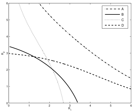
Figure 2: The rate region for a $2$-user interference channel with the following constraints on the power, A: $p_{1}\geq 0$, $p_{2}\geq 0$, B: $p_{1}+p_{2}\geq\bar{p}_{t}$, $p_{1}\geq 0$, $p_{2}\geq 0$ C: $0\leq p_{1}\leq\bar{p}_{1}$, $p_{2}\geq 0$, D: $0\leq p_{2}\leq\bar{p}_{2}$, $p_{1}\geq 0$

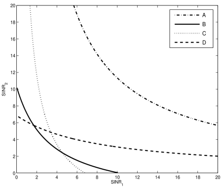
Figure 3: The rate region for a $2$-user interference channel with the following constraints on the power, A: $p_{1}\geq 0$, $p_{2}\geq 0$, B: $p_{1}+p_{2}\geq\bar{p}_{t}$, $p_{1}\geq 0$, $p_{2}\geq 0$ C: $0\leq p_{1}\leq\bar{p}_{1}$, $p_{2}\geq 0$, D: $0\leq p_{2}\leq\bar{p}_{2}$, $p_{1}\geq 0$

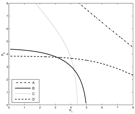
Figure 4: The rate region for a $2$-user interference channel with the following constraints on the power, A: $p_{1}\geq 0$, $p_{2}\geq 0$, B: $p_{1}+p_{2}\geq\bar{p}_{t}$, $p_{1}\geq 0$, $p_{2}\geq 0$ C: $0\leq p_{1}\leq\bar{p}_{1}$, $p_{2}\geq 0$, D: $0\leq p_{2}\leq\bar{p}_{2}$, $p_{1}\geq 0$

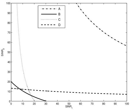
Figure 5: The rate region for a $2$-user interference channel with the following constraints on the power, A: $p_{1}\geq 0$, $p_{2}\geq 0$, B: $p_{1}+p_{2}\geq\bar{p}_{t}$, $p_{1}\geq 0$, $p_{2}\geq 0$ C: $0\leq p_{1}\leq\bar{p}_{1}$, $p_{2}\geq 0$, D: $0\leq p_{2}\leq\bar{p}_{2}$, $p_{1}\geq 0$

The rate region is simply the intersection of all the rate regions resulted from applying each constraint separately. As shown in Fig. 2 and Fig. 3, the boundary of SINR and rate region, when there is no upper-bound on powers is always above other boundaries. It is because of the fact that the maximum achievable SINR for the unbounded-power system is the inverse of PF-eigenvalue of $\mathrm{diag}{(\boldsymbol{\mu})}\mathbf{A}$; while the maximum achievable SINR when the power is bounded, is the inverse of PF-eigenvalue of a matrix which is definitely greater than $\mathrm{diag}{(\boldsymbol{\mu})}\mathbf{A}$. Therefore, based on Theorem 1 the unbounded SINR boundary would be above the bounded-power systems. Thus, this boundary doesn’t have any direct role in forming the main boundary. An interesting observation is that if the $\overline{p}_{i}$’s or $\overline{p}_{t}$ are increased the boundaries of bounded-power systems tend to the unbounded-power system boundary; the extreme case is when the maximum power goes to infinity which means the power is unbounded, then the matrices whose inverse of PF-eigenvalue form the boundaries become equal and these boundaries touch each other.

As another observation, the rate and SINR regions for a 2-user channel with weaker cross links are shown in Fig. 4 and 5. The gain matrix in this system is assumed to be

$$\mathbf{G}=\left[\begin{array}[]{ll}2.0430&0.0359\\ 0.0134&1.3313\end{array}\right],$$ (24)

while the power of individual users and the total power are upper-bounded as $\overline{p}_{1}=1,\quad\overline{p}_{2}=1,\quad\overline{p}_{t}=1.5$, and $\sigma_{1}^{2}=\sigma_{2}^{2}=10^{-1}$. The extreme point of this situation is when the links have no interference on each other and therefore the maximum SINR for each user considering the individual constraints would be $SINR_{i}=\dfrac{\overline{p}_{i}g(i,i)}{\sigma^{2}}$ for each user. We can see in Fig. 4 and Fig. 5 that these boundaries are more straight than the ones in Fig. 2 and Fig. 3 which confirms our conjecture.

IV Time-Varying Channel

So far, we have assumed that the channel gains are fixed with time. However, in practice, channel gains vary with time due to the users’ movement or changing the environment conditions.

In this section, we consider an interference channel with $n$ co-channel links whose channel gain matrix is randomly selected from a finite set $\{\mathbf{G}_{1},\ldots,\mathbf{G}_{l}\}$ with probability $\rho_{1},\ldots,\rho_{l}$, respectively. The matrix $\mathbf{A}_{i}$ denotes the normalized gain matrix in the state $i$, $i\in\{1,\ldots,l\}$. The objective is to find the maximum $\gamma$ which is achievable by all users in all channel states, while the average power of the users are constrained, i.e.,

$$\max{\gamma}$$

$$\mathrm{s.t.}\quad \gamma_{j+(i-1)n}\geq\mu_{j}\gamma,\quad\forall j\in\Omega,i\in\{1,\ldots,l\}$$

$$p_{j+(i-1)n}\geq 0,\quad\forall j\in\Omega,i\in\{1,\ldots,l\}$$ (25)

$$\displaystyle E[\sum_{j\in\Omega}{p_{j+(i-1)n}}]\leq\overline{p}_{\Omega},$$ (26)

where $\gamma_{j+(i-1)n}$ and $p_{j+(i-1)n}$ are the SINR and the power of transmitter $j$ respectively, when the channel gain matrix is $\mathbf{G}_{i}$. We define an expanded system including $ln$ users with block diagonal matrices $\mathbf{G}$ and $\mathbf{A}$ as the channel gain matrix and the normalized gain matrix, respectively. In the matrices $\mathbf{G}$ and $\mathbf{A}$, the $i^{th}$ matrix on the diagonal is $\mathbf{G}_{i}$ and $\mathbf{A}_{i}$, respectively. It is clear that block diagonal format of these matrices indicate that there is no interference between the links associated with different states. Like the previous discussions the requirements on these links form a system of linear equations with the following formulation in a matrix form,

$$(\dfrac{1}{\gamma}\mathbf{I}_{ln\times ln}-\mathrm{diag}{(\mathbf{1}_{l\times 1}\otimes\boldsymbol{\mu})}\mathbf{A})\mathbf{p}=\boldsymbol{\eta},$$ (27)

where

$$\eta_{j+(i-1)n}=\dfrac{\mu_{j}\sigma^{2}_{j}}{g_{j+(i-1)n,j+(i-1)n}},j\in\Omega,i\in\{1,\ldots,l\}.$$

According to (9), we define $\mathbf{F}$ as

$$\mathbf{F}=\dfrac{1}{\gamma}\mathbf{I}_{ln\times ln}-\mathrm{diag}{(\mathbf{1}_{l\times 1}\otimes\boldsymbol{\mu})}\mathbf{A}.$$

Then, we have

$$\mathbf{F}\mathbf{p}=\gamma\boldsymbol{\eta}.$$

Using Cramer’s rule, we will have

$$p_{j+(i-1)n}=\dfrac{\det(\mathbf{H}^{(j+(i-1)n)})}{\det(\mathbf{F})},$$

where $\mathbf{H}^{(j+(i-1)n)}$ according to (11) is the matrix $\mathbf{F}$ whose column $j+(i-1)n$ is substituted by $\gamma\boldsymbol{\eta}$. The average of the total power of the users in $\Omega$ is equivalent to

$$\displaystyle E_{i}\sum_{j\in\Omega}{p_{j+(i-1)n}} =\displaystyle\sum_{i=1}^{l}{\rho_{i}\displaystyle\sum_{j\in\Omega}{p_{j+(i-1)n}}}$$

$$=\displaystyle\sum_{i=1}^{l}{\rho_{i}\displaystyle\sum_{j\in\Omega}{\dfrac{\det(\mathbf{H}^{(j+(i-1)n)})}{\det(\mathbf{F})}}}$$

$$=\dfrac{1}{\det(\mathbf{F})}\displaystyle\sum_{i=1}^{l}{\rho_{i}\displaystyle\sum_{j\in\Omega}{\det(\mathbf{H}^{(j+(i-1)n)})}}.$$ (28)

Based on (28), we define

$$\mathrm{u}_{\Omega}(\gamma)=\overline{p}_{\Omega}\det(\mathbf{F})-\displaystyle\sum_{i=1}^{l}{\rho_{i}\displaystyle\sum_{j\in\Omega}{\det(\mathbf{H}^{(j+(i-1)n)})}},$$

and

$$\mathrm{f}(\gamma)=\det(\mathbf{F}).$$

Therefore, the constraint in (26) is equivalent to

$$\dfrac{\mathrm{u}_{\Omega}(\gamma)}{\mathrm{f}(\gamma)}\geq 0.$$

Like before, it is easy to show that the maximum achievable SINR satisfying constraints (25) and (26) is

$$\gamma^{*}=\min{\{r(\mathrm{f}),r(\mathrm{u}_{\Omega})\}}.$$ (29)

To simplify $\mathrm{u}_{\Omega}(\gamma)$, we have

$$\mathrm{u}_{\Omega}(\gamma) =\overline{p}_{\Omega}\det(\mathbf{F})-\displaystyle\sum_{i=1}^{l}{\rho_{i}\displaystyle\sum_{j\in\Omega}{\det(\mathbf{H}^{(j+(i-1)n)})}}$$

$$=\overline{p}_{\Omega}(\det(\mathbf{F})-\displaystyle\sum_{i=1}^{l}{\displaystyle\sum_{j\in\Omega}{\det(\mathbf{\hat{H}}^{(j+(i-1)n)})}}),$$

where $\mathbf{\hat{H}}^{(j+(i-1)n)}$ is $\mathbf{{H}}^{(j+(i-1)n)}$ whose column $j+(i-1)n$ is multiplied by $\dfrac{\rho_{i}}{\overline{p}_{\Omega}}$. Using the same procedure as before, we obtain

$$\mathrm{u}_{\Omega}(\gamma)=\overline{p}_{\Omega}\det{(\mathbf{F}-\mathbf{D})},$$

where

$$\mathbf{D}=\displaystyle\sum_{i=1}^{l}{\psi(\mathbf{0}_{ln\times ln},\dfrac{\rho_{i}\gamma\boldsymbol{\eta}}{\overline{p}_{\Omega}},\{j+(i-1)n:j\in\Omega\})}$$

It is easy to see that

$$r(\mathrm{u}_{\Omega})=\dfrac{1}{\lambda^{*}\big{(}\mathrm{diag}{(\mathbf{1}_{l\times 1}\otimes\boldsymbol{\mu})}\mathbf{A}+\displaystyle\sum_{i=1}^{l}{\psi(\mathbf{0}_{ln\times ln},\dfrac{\rho_{i}\boldsymbol{\eta}}{\overline{p}_{\Omega}},\{j+(i-1)n:j\in\Omega\})}\big{)}}.$$

and

$$r(\mathrm{f})=\dfrac{1}{\lambda^{*}(\mathrm{diag}{(\mathbf{1}_{l\times 1}\otimes\boldsymbol{\mu})}\mathbf{A})}.$$

Therefore, using Theorem 1 and equation (29), we will have the following theorem.

Theorem 3

The maximum achievable $\gamma$ in a time-varying interference channel with $n$ links and probability vector $\boldsymbol{\rho}_{l\times 1}$, with the following constraints on power,

$$p_{j,i}\geq 0,\forall j\in\Omega,i\in\{1,\ldots,l\},\quad$$

$$\displaystyle E[\sum_{j\in\Omega}{p_{j,i}}]\leq\overline{p}_{\Omega}$$

is equal to

$$\gamma^{*}=\dfrac{1}{\lambda^{*}\big{(}\mathrm{diag}{(\mathbf{1}_{l\times 1}\otimes\boldsymbol{\mu})}\mathbf{A}+\displaystyle\sum_{i=1}^{l}{\psi(\mathbf{0}_{ln\times ln},\dfrac{\rho_{i}\boldsymbol{\eta}}{\overline{p}_{\Omega}},\{j+(i-1)n:j\in\Omega\})}\big{)}}.$$

Apparently, if there are multiple constraints on the power, the maximum achievable SINR $\gamma^{*}$ is computed by

$$\gamma^{*}=\displaystyle\min_{i}{\gamma^{*}_{i}},$$

where $\gamma^{*}_{i}$ is the maximum achievable SINR obtained by Theorem 3 while only the constraint $i$ is considered for the system.

V Conclusion

In this paper, we have obtained a closed-form solution for the maximum achievable SINR in an interference channel, utilizing the Perron-Frobenious theorem, when there is a total power constraint on any subset of the users. This result leads to characterizing the boundary of the rate region with multiple constraints on the power. In addition, we considered a time-varying interference channel where the average of total power of an arbitrary subset of the transmitters is subject to an upper-bound. A closed-form expression for the rate-region of such a channel is obtained and extended to the systems with multiple power constraints.

References

[1]
J.M. Aein,
“Power balancing in systems employing frequency reuse,”
in Comsat Tech. Rev., 1973, vol. 3.
[2]
H. Alavi and R. W. Nettleton,
“Downstream power control for a spread spectrum celular mobile radio
system,”
in IEEE GLOBECOM, 1982, pp. 84 – 88.
[3]
J. Zander,
“Performance of optimum transmitter power control in cellular radio
systems,”
IEEE Transactions on Vehicular Technology, vol. 41, no. 1, pp.
57 – 62, February 1992.
[4]
J. Zander,
“Distributed cochannel interference control in cellular radio
systems,”
IEEE Transactions on Vehicular Technology, vol. 41, no. 3, pp.
305 – 311, August 1992.
[5]
D.N.C. Tse and S.V. Hanly,
“Linear multiuser receivers: effective interference, effective
bandwidth and user capacity,”
Automatica, vol. 35, no. 12, pp. 19872012, March 1999.
[6]
D. Catrein, L.A. Imhof, and R. Mathar,
“Power control, capacity, and duality of uplink and downlink in
cellular CDMA systems,”
IEEE Transactions on Communications, vol. 52, no. 10, pp. 1777
– 1785, October 2004.
[7]
L.A. Imhof and R. Mathar,
“Capacity regions and optimal power allocation for CDMA cellular
radio,”
IEEE Transactions on Information Theory, vol. 51, no. 6, pp.
2011 – 2019, June 2005.
[8]
H. Boche and S. Stanczak,
“Convexity of some feasible QoS regions and asymptotic behavior of
the minimum total power in CDMA systems,”
IEEE Transactions on Communications, vol. 52, no. 12, pp. 2190
– 2197, December 2004.
[9]
H. Boche and S. Stanczak,
“Log-convexity of the minimum total power in CDMA systems with
certain quality of- service guaranteed,”
IEEE Transactions on Information Theory, vol. 51, no. 1, pp.
374381, January 2005.
[10]
R. Cruz and A. Santhanam,
“Optimal routing, link scheduling and power control in multi-hop
wireless networks,”
in 22nd IEEE Conf. Comput. Commun., San Francisco, CA,
March-April 2003.
[11]
C. W. Sung,
“Log-convexity property of the feasible SIR region in
power-controlled cellular systems,”
IEEE Communications Letters, vol. 6, no. 6, pp. 248 249, June
2002.
[12]
S. Stanczak and H. Boche,
“The infeasible SIR region is not a convex set,”
IEEE Transactions on Communications, vol. 54, no. 11, pp. 1905
– 1907, November 2006.
[13]
E. Seneta,
Non-Negative Matrices: An Introduction to Theory and
Applications,
John Wiley and Sons, January 1973.
[14]
M. Chiang,
“Geometric programming for communication systems,”
Foundations and Trends of Communications and Information
Theory, vol. 2, no. 1-2, pp. 1–156, August 2005.
[15]
D. Julian, M. Chiang, D. O’Neill, and S. Boyd,
“QoS and fairness constrained convex optimization of resource
allocation for wireless cellular and ad hoc networks,”
in IEEE Infocom, Twenty-First Annual Joint Conference of the
IEEE Computer and Communications Societies, June 2002, vol. 2, pp. 477–486.