Contains and Inside relationships within Combinatorial Pyramids

Abstract

Irregular pyramids are made of a stack of successively reduced graphs embedded in the plane. Such pyramids are used within the segmentation framework to encode a hierarchy of partitions. The different graph models used within the irregular pyramid framework encode different types of relationships between regions. This paper compares different graph models used within the irregular pyramid framework according to a set of relationships between regions. We also define a new algorithm based on a pyramid of combinatorial maps which allows to determine if one region contains the other using only local calculus.

,

1 Introduction

Graphs play an important role in computer vision and pattern recognition since the birth of these fields. Graphs are used along the overall process from the stimuli to the interpretation task: hierarchical and non-hierarchical data structures for image segmentation, graph matching for pattern recognition, graph clustering for structural classification, and computation of a median graph [1] for learning the structural properties of models.

Graphs are thus used both for low level image processing and high level tasks. Different type of graphs being used for different types of applications. However, in many computer vision tasks, the low image segmentation stage cannot be readily separated from higher level processing. On the contrary, the segmentation algorithms should often extract fine information about the partition in order to guide the segmentation process according to the high level goal. This information may be used to compare isolated regions or some local configuration of regions to a model. There is thus a need to design graph models for image segmentation which can be both efficiently updated and allow to extract fine information about the partition.

1.1 Relating Regions

Different formalisms such as the RCC-8 defined by Randel [2] or the relationships defined by K. Shearer et al. [3] in the context of graph matching may be used to relate the regions of a partition. Within the particular context of image segmentation, the following relationships may be defined from these two models:meets, contains, inside:

1. The meets relationship means that two regions share at least one common boundary. The different models used to encode partitions either encode the existence of this common boundary or create one relationship for each boundary between two regions. We denote these two types of encodings meets_exists and meets_each. The ability of the models to retrieve efficiently a given common boundary between two regions is also an important feature of these models.

2. The relationship A contains B expresses the fact that region B is inside region A. For example, the background of the road sign in Fig. 1(a) contains the upside arrow.

3. The inside relationship is the inverse of the contains relation: A region B inside A is contained in A.

One additional relationship not directly handled by the models of Shearer and Randel may be defined within the hierarchical segmentation scheme. Indeed within such a framework a region defined at a given level of a hierarchy is composed of regions defined at levels below.

The following relationships may thus be deduced from the relationships defined by Shearer and Randel: The meets_exists, meets_each, contains, inside and composed of. Note that unlike meets relationships, the contains and inside relations are asymmetric. A contains or inside relation between two regions allows thus to characterize each of the regions sharing this relation.

1.2 Region Adjacency Graph

One of the most common graph data structure, within the segmentation framework is the Region Adjacency Graph (RAG). A RAG is defined from a partition by associating one vertex to each region and by creating an edge between two vertices if the associated regions share a common boundary. A RAG corresponds thus to a simple graph without any double edge between vertices nor self-loop. Within a non-hierarchical segmentation scheme the RAG model is usually applied as a merging step to overcome the over-segmentation produced by the previous splitting algorithm [4]. Indeed, the existence of an edge between two vertices denotes the existence of at least one common boundary segment between the two associated regions which may thus be merged by removing this segment. Within this framework, the edge information may thus be interpreted as a possibility to merge the two regions identified by the vertices incident to the edge. Such a merge operation implies to collapse the two vertices incident to the edge into one vertex and to remove this edge together with any double edge between the newly created vertex and the remaining vertices.

The RAG model encodes thus only the existence of a common edge between two regions (the meets_exists relationship). Moreover, the existence of a common edge between two vertices does not provide enough information to differentiate a meets relationship from a contains or inside one. This drawback is illustrated on an ideal segmentation of two roadsigns (Fig. 1) which are encoded by a same RAG. The road sign (a) defines two nested contains relationships. Indeed, the white border contains the background which contains itself the symbol. On the other hand the road sign (b) corresponds to two meets relationships between the central region and its two white neighbors.

1.3 Combinatorial Maps

A 2D combinatorial map may be understood as a planar graph encoding explicitly the orientation in the plane. Each connected component of a partition (a connected set of regions) may be encoded by a 2D combinatorial map up to an homeomorphism [5]. One of the main insight of such models compared to a RAG data structure is their ability to be efficiently updated after both split and merge operations.

The combinatorial map formalism allows to encode each connected boundary between two regions by one edge. The models based on combinatorial maps encode thus the meets_each relationship. However, within the combinatorial map framework two connected components of a partition will be encoded by two combinatorial maps without any information about the respective positioning of the two components. The models based on combinatorial maps have thus designed additional data structure like the inclusion tree [6] or the Parent-Child relationships [5, 7] to encode the contains and inside relationships. Using these models any modification of the partition implies to update both the combinatorial maps and the additional data structures.

1.4 Segmentation Hierarchies

Data structures used within the hierarchical segmentation framework encode a stack of partitions successively simplified by region merging. Irregular pyramids models introduced by Meer and Montanvert [8] encode each partition by a graph where each vertex is associated to one region. At each level of the pyramid a region is obtained by the merge of a connected set of regions at the level below. The resulting region is called the parent of the merged regions. These last regions correspond to the child of the region at the level above. The models based on the irregular pyramid framework encode thus naturally the composed of relationship. In order to preserve the efficiency of a hierarchical data structure, the size of models encoding each partition of the hierarchy must be strictly decreasing according to the level. This last constraint forbids the use of an additional data structure similar to the structures used for combinatorial maps models in order to store contains and inside relationships. Indeed, contains and inside relationships between regions may both be removed and created along the different levels of the pyramid. The use of such an additional data structure may thus violate the strictly decreasing size of the models according to the levels.

1.5 Overview

The aim of this paper is twofold: We firstly provide an introduction to the main data structures used within the hierarchical segmentation framework according to the set of relationships previously defined (Section 1.1). Secondly, we present an efficient computation of the contains and inside relationships within the irregular pyramid framework. The remaining of this paper is thus organized as follows: Section 2 presents two models belonging to the irregular pyramid framework together with their properties relative to the relationships previously defined. Section 3 describes the combinatorial map model and its main properties. Section 4 describes the construction scheme and the main properties of a pyramid of combinatorial maps : A combinatorial Pyramid. Finally, Section 5 presents one algorithm computing the contains and inside information using only local calculus.

2 Simple and Dual Graph Pyramids

The irregular pyramids are defined as a stack of successively reduced graphs, each graph being built from the graph below by selecting a set of vertices named surviving vertices and mapping each non-surviving vertex to a surviving vertex [9, 8]. Using such a framework, the graph $G_{l+1}=(V_{l+1},E_{l+1})$ defined at level $l+1$ is deduced from the graph defined at level $l$ by the following steps:

1. Select the vertices of $G_{l+1}$ among $V_{l}$. These vertices are the surviving vertices of the decimation process, $V_{l+1}\subset V_{l}$.

2. Each non-surviving vertex connects to a surviving vertex by one edge of $G_{l}$. The set of vertices attached to each surviving vertex defines a partition of $V_{l}$.

3. Define the adjacency relationships between the vertices of $G_{l+1}$ in order to define $E_{l+1}$.

2.1 Simple graph Pyramids

In order to obtain a decimation ratio greater than 1 between two successive levels, Meer [9] imposes the following constraints on the set of surviving vertices:

$$\forall v\in V_{l}-V_{l+1}\;\exists v^{\prime}\in V_{l+1}:\;(v,v^{\prime})\in E_{l}$$ (1)

$$\forall(v,v^{\prime})\in V_{l+1}^{2}:\;(v,v^{\prime})\not\in E_{l}$$ (2)

Constraint (1) insures that each non-surviving vertex is adjacent to at least a surviving vertex. Constraint (2) insures that two adjacent vertices cannot both survive. These constraints define a maximal independent set (MIS) [9, 8].

Given the set of surviving vertices, different methods [8, 10] may be used to link each non-surviving vertex to one of its surviving neighbor. For example, Montanvert [8] attaches each non-surviving vertex to its closest surviving neighbor according to a difference between the outcome of a random variable attached to each vertex. The set of non-surviving vertices connected to a surviving vertex defines its reduction window and thus the parent child relationship between two consecutive levels.

The final set of surviving vertices defined on $V_{l}$ corresponds to the set of vertices $V_{l+1}$ of the reduced graph $G_{l+1}=(V_{l+1},E_{l+1})$. The set of edges $E_{l+1}$ of $G_{l+1}$ is defined by connecting by an edge in $G_{l+1}$ any couple of surviving vertices having adjacent children.

Two surviving vertices are thus connected in $G_{l+1}$ if they are connected in $G_{l}$ by a path of length lower or equal than $3$. Two reduction windows adjacent by more than one path of length lower or equal than $3$ will thus be connected by a single edge in the reduced graph. The stack of graphs produced by the above decimation process is thus a stack of simple graphs each simple graph encoding only the existence of one common boundary between two regions (the meeets_exists relationship). Moreover, as mentioned in Section 1.2 the RAG model which corresponds to a simple graph does not allow to encode contains and inside relationships.

2.2 Construction of Dual Graph Pyramids

The dual graph pyramids introduced by Willersinn and Kropatsch [11] use an alternative construction scheme. Within the dual graph pyramid framework the reduction process is performed by a set of edge contractions. The edge contraction collapses two adjacent vertices into one vertex and removes the edge. Many edges except self-loops can be contracted independently of each other and also in parallel. In order to avoid contracting a self-loop these edges should not form cycles, e.g. form a forest. This set of edges is called a contraction kernel.

The contraction of a graph reduces the number of vertices while maintaining the connections to other vertices. As a consequence some redundant edges may occur. These edges belong to one of the following categories:

• Redundant double edge: These edges encode multiple adjacency relationships between two vertices and define degree two faces. They can thus be characterized in the dual graph as degree two dual vertices. In terms of partition’s encoding these edges correspond to an artificial split of one boundary between two regions.

• Empty self-loop: These edges correspond to a self-loop with an empty inside. These edges define thus degree one faces and are characterized in the dual graph as degree one vertices. Such edges encode artificial inner boundaries of regions.

Both double edges and empty self-loops do not encode relevant topological relations and can be removed without any harm to the involved topology [11]. The removal of such edges is called a dual decimation step and the set of removed edges is called a removal kernel. Such a kernel defines a forest of the dual graph.

2.3 Dual Graph Pyramids and multiple boundaries

Given one tree of a contraction kernel, the contraction of its edges collapses all the vertices of the tree into a single vertex and keeps all the connections between the vertices of the tree and the remaining vertices of the graph. The multiple boundaries between the newly created vertex and the remaining vertices of the graph are thus preserved. Each graph of a dual graph pyramid encodes thus the meets_each relationships. This property is not modified by the application of a removal kernel which only removes redundant edges.

2.4 Dual Graph Pyramids and the inside relationship

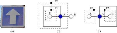
Figure 2: The Graph (b) defines the top of a dual graph pyramid encoding an ideal segmentation of (a). The self loop incident to vertex A may surround either vertex B or C without changing the incidence relations between vertices and faces. The dual vertices associated to faces are represented by filled boxes ($\blacksquare$). Dual edges are represented by dashed lines.

Due to the forest requirement, the encoding of the adjacency between two regions one inside the other will be encoded by two edges (Fig. 2): One edge encoding the common border between the two regions and one self-loop incident to the vertex encoding the surrounding region. One may think to characterize the inside relationship by the fact that the vertex associated to the inside region should be surrounded by the self-loop. However, as shown by Fig. 2(c) one may exchange the surrounded vertex without modifying the incidence relationships between both vertices and faces. Two dual graphs being defined by these incidence relationships one can exchange the surrounded vertex without modifying the encoding of the graphs. This last remark shows that the inside/contains relationships cannot be characterized locally within the dual graph framework.

3 Combinatorial maps

Combinatorial maps and generalized combinatorial maps define a general framework which allows to encode any subdivision of nD topological spaces orientable or non-orientable with or without boundaries. Recent trends in combinatorial maps apply this framework to the segmentation of 3D images [12, 13] and the encoding of 2D [14, 15] and nD [16] hierarchies.

The remaining of this paper will be based on 2D combinatorial maps which will be just called combinatorial maps. A combinatorial map may be deduced from a planar graph by splitting each edge into two half edges called darts. An edge connecting two vertices is thus composed of two darts, each dart belonging to only one vertex. The relation between two darts $d_{1}$ and $d_{2}$ associated to the same edge is encoded by the permutation $\alpha$ which maps $d_{1}$ to $d_{2}$ and $d_{2}$ to $d_{1}$. The permutation $\alpha$ is thus an involution and its cycles are denoted by $\alpha^{*}(d)$ for a given dart $d$. These cycles encode the edges of the graph. The sequence of darts encountered when turning around a vertex is encoded by the permutation $\sigma$. Using a counter-clockwise orientation, the cycle $\sigma^{*}(d)$ encodes the set of darts encountered when turning counter-clockwise around the vertex encoded by the dart $d$. A combinatorial map can thus be formally defined by $G=(\mbox{$\mathcal{D}$}{},\sigma,\alpha)$, where $\mathcal{D}$ is the set of darts and $\sigma$, $\alpha$ are two permutations defined on $\mathcal{D}$ such that $\alpha$ is an involution.

Given a combinatorial map $G=(\mbox{$\mathcal{D}$},\sigma,\alpha)$, its dual is defined by $\mbox{$\overline{G}$}=(\mbox{$\mathcal{D}$},\varphi,\alpha)$ with $\varphi=\sigma\circ\alpha$. The cycles of the permutation $\varphi$ encode the set of darts encountered when turning around a face of $G$.

We can state one of the major difference between a combinatorial map and an usual graph encoding of a partition. Indeed, a combinatorial map may be seen as a planar graph with a set of vertices (the cycles of $\sigma$) connected by edges (the cycles of $\alpha$). However, compared to an usual graph encoding a combinatorial map encodes additionally the local orientation of edges around each vertex thanks to the order defined within each cycle of $\sigma$.

Fig. 3 illustrates the encoding of a $3\times 3$ $4$-connected discrete grid by a combinatorial map $G$. The involution $\alpha$ is implicitly encoded by the sign in Fig. 3(a) and (b). We have thus $\alpha(d)=-d$ for all darts on these figures.

Since $G$ encodes a planar sampling grid, each vertex of $\overline{G}$ (Fig. 3(b)) is associated to a corner of a pixel. For example, the top left pixel of the $3\times 3$ grid is encoded by the $\sigma$ cycle $\sigma^{*}(1)=(1,13,24,7)$ (top left vertex and square in Fig. 3(a) and (b)). The top-left corner of this pixel is encoded by the $\varphi$ cycle: $\varphi^{*}(24)=(24,-13)$ (top left dual vertex of Fig. 3(b)). Moreover, each dart may be understood in this combinatorial map as an oriented crack, i.e. as a side of a pixel with an orientation. For example, the dart $1$ in Fig. 3(b) encodes the right side of the upper-left pixel oriented from bottom to top. The $\varphi$, $\alpha$ and $\sigma$ cycles of a dart may thus be respectively understood as elements of dimensions $0$, $1$ and $2$.

Each dart of a combinatorial map $G$, encoding a planar sampling grid may thus be interpreted as an oriented crack and associated to a point encoding the coordinates of a pixel’s corner and one move encoding the orientation on the crack associated to the dart.

4 Embedding and Orientation

As in the dual graph pyramid scheme [17] (Section 2) a combinatorial pyramid is defined by an initial combinatorial map successively reduced by a sequence of contraction or removal operations. The initial combinatorial map encodes a planar sampling grid (Section 3) or a first segmentation and the remaining combinatorial maps of a combinatorial pyramid encode a stack of image partitions successively reduced. Such combinatorial maps are thus embedded (Section 4.3). As mentioned in Section 3 a combinatorial map may be understood as a dual graph with an explicit encoding of the orientation of the edges incident to each vertex. This explicit encoding of the orientation is preserved within the combinatorial pyramid using contraction and removal operations equivalent to the operations used for dual graphs but which preserve the orientations of edges around the vertices of the reduced combinatorial maps [14, 15].

Contraction operations are controlled by contraction kernels (CK). The removal of redundant edges is performed as in the dual graph reduction scheme by a removal kernel. This kernel is however decomposed in two sub-kernels : A removal kernel of empty self-loops (RKESL) which contains all darts incident to a degree 1 dual vertex and a removal kernel of empty double edges (RKEDE) which contains all darts incident to a degree 2 dual vertex. These two removal kernels are defined as follows : The removal kernel of empty self-loops RKESL is initialized by all self-loops surrounding a dual vertex of degree 1. RKESL is further expanded by all self-loops that contain only other self-loops already in RKESL until no further expansion is possible. For the removal of empty double edges RKEDE we ignore all empty self-loops in RKESL in computing the degree of the dual vertex. Note that the successive application of a RKESL and a RKEDE is equivalent to the application of a removal kernel defined within the dual graph framework. Both contraction and removal operations defined within the combinatorial pyramid framework are thus defined as is the dual graph framework but additionally preserve the orientation of edges around each vertex. Further details about the construction scheme of a Combinatorial Pyramid may be found in [14].

4.1 What is inside ?

Combinatorial pyramids are thus built using the same framework as dual graphs pyramids. The use of a contraction kernel within the construction scheme of a combinatorial pyramid allows to encode multiple adjacency between regions thanks to multiple edges between their associated vertices. Therefore, as in the dual graph framework, combinatorial pyramids preserve the meets_each relationship (Section 2.3). Note that the explicit encoding of the orientation within the combinatorial pyramid framework does not interfere with this last property.

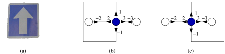
Figure 4: The encoding of an ideal segmentation of a road sign (a) by the top level combinatorial map of a pyramid may be drawn using either (b) or (c).

Moreover, as in the dual graph framework (Section 2.4), an inside relationship between two regions is encoded by two edges: one edge encodes the common border between the two regions while the other encodes a self-loop incident to the vertex associated to the surrounding region. Let us consider the example already used for dual graph pyramids (Section 2.4, Fig. 2). Fig. 4 shows the encoding of the ideal segmentation of the road sign using combinatorial maps. As shown by Fig. 4 (b) and (c), one can exchange the surrounded vertex without changing the order of the darts around the vertex $\sigma^{*}(1)$. Therefore, the two drawings shown in Fig. 4(b) and (c) are encoded by the same combinatorial map. One cannot determine from the formally specified combinatorial map which part is inside and which is contained. This ambiguity may also be characterized using the cycle $\sigma^{*}(1)$ of the vertex incident to the self-loop. Indeed, this cycle is equal to $\sigma^{*}(1)=(1,2,-1,3)$. Since $(1,-1)$ is a self-loop the neighbors of $\sigma^{*}(1)$ have in their $\sigma$ cycles the $\alpha$ successors of the two darts $2$ and $3$. The ambiguity about the drawing of the self-loop is characterized on the cycle $\sigma^{*}(1)$ by the fact that we can not deduce from this cycle if the dart $2$ is between $1$ and $-1$ or if on the contrary $3$ is between $-1$ and $1$. This ambiguity arises thus because the two darts $1$ and $-1$ play a symmetric role in $\sigma^{*}(1)$. We can thus state the two following points from the above discussion:

1. Combinatorial pyramids preserve the meets_each relationship.

2. An inside relationship ’A inside B’ is always associated with a self-loop incident to B. However, a non-redundant self-loop at B does not always identify the inside region.

4.2 Implicit encoding of a combinatorial pyramid

Let us consider an initial combinatorial map $G_{0}=(\mbox{$\mathcal{D}$},\sigma,\alpha)$ and a sequence of kernels $K_{1},\dots,K_{n}$ successively applied on $G_{0}$ to build the pyramid. Each combinatorial map $G_{i}=(\mbox{$\mathcal{SD}$}_{i},\sigma_{i},\alpha_{i})$ is defined from $G_{i-1}=(\mbox{$\mathcal{SD}$}_{i-1},\sigma_{i-1},\alpha_{i-1})$ by the application of the kernel $K_{i}$ on $G_{i-1}$ and the set of darts $\mbox{$\mathcal{SD}$}_{i}$ is equal to $\mbox{$\mathcal{SD}$}_{i-1}\setminus K_{i}$. We have thus:

$$\mbox{$\mathcal{SD}$}_{n+1}\subset\mbox{$\mathcal{SD}$}_{n}\subset\dots\mbox{$\mathcal{SD}$}_{1}\subset\mbox{$\mathcal{D}$}$$ (3)

The set of darts of each reduced combinatorial map of a pyramid is thus included in the base level combinatorial map. This last property allows us to define the two following functions:

1. one function $state$ from $\{1,\dots,n\}$ to the states $\{CK,RKESL,RKEDE\}$ which specifies the type of each kernel.

2. One function $level$ defined for all darts in $\mathcal{D}$ such that $level(d)$ is equal to the maximal level where $d$ survives:

   $$\forall d\in\mbox{$\mathcal{D}$}\;level(d)=\begin{array}[t]{r}Max\{i\in\{1,\dots,n+1\}\,|\,d\in\mbox{$\mathcal{SD}$}_{i-1}\}\\ \end{array}$$

   a dart $d$ surviving up to the top level has thus a level equal to $n+1$. Note that if $d\in K_{i},i\in\{1,\dots,n\}$ then $level(d)=i$.

We have shown [10, 14] that the sequence of reduced combinatorial maps $G_{0},\dots,G_{n+1}$ may be encoded without any loss of information using only the base level combinatorial map $G_{0}$ and the two functions $level$ and $state$. Such an encoding is called an implicit encoding of the pyramid.

The receptive field of a dart $d\in\mbox{$\mathcal{SD}$}_{i}$ corresponds to the set of darts reduced to $d$ at level $i$ [14, 10]. Using the implicit encoding of a combinatorial pyramid, the receptive field $RF_{i}(d)$ of $d\in\mbox{$\mathcal{SD}$}_{i}$ is defined as a sequence $d_{1}.\dots.d_{q}$ of darts in $\mathcal{D}$ by $d_{1}=d$, $d_{2}=\sigma_{0}(d)$ and for each $j$ in $\{3,\dots,q\}$ :

$$d_{j}=\left\{\begin{array}[]{ll}\varphi_{0}(d_{j-1})&\mbox{if }state(level(d_{j-1}))=CK\\ \sigma_{0}(d_{j-1})&\mbox{if }state(level(d_{j-1}))\in\{RKEDE,RKESL\}\\ \end{array}\right.$$ (4)

The dart $d_{q}$ is defined as the last dart of the sequence which have been contracted or removed below the level $i$. Therefore, the successor of $d_{q}$ according to equation 4, $d_{q+1}$ satisfies $level(d_{q+1})>i$. Moreover, we have shown [14, 10] that $d$, $d_{q}$ and $d_{q+1}$ are additionally connected by the two following relationships:

$$\sigma_{i}(d)=d_{q+1}\mbox{ and }\alpha_{i}(d)=\alpha_{0}(d_{q})$$ (5)

Note that these two last relationships allow to retrieve any reduced combinatorial map of the pyramid from its base.

The implicit encoding of combinatorial pyramids is thus based on the fact that the set of darts of any reduced combinatorial map is included in the initial combinatorial map (equation 3). The two functions $state$ and $level$ which are based on this property allow to encode the whole sequence of reduced combinatorial map without loss of information [14, 10].

4.3 Dart’s embedding and Segments

In the RAG a region corresponds to a vertex and two regions are connected by an edge if the two regions share a boundary. In the Combinatorial Map, vertices and edges correspond to $\sigma$ and $\alpha$ cycles respectively. Therefore, each dart $d\in\mbox{$\mathcal{SD}$}_{i}$ encodes a boundary between the regions associated to $\sigma_{i}^{*}(d)$ and $\sigma_{i}^{*}(\alpha_{i}(d))$. Moreover, in the lower levels of the pyramid the two vertices of an edge may belong to a same region. We call the corresponding boundary segment an internal boundary in contrast to an external boundary which separates two different regions of a RAG. The receptive field of $d$ at level $i$ ($RF_{i}(d)$) contains both darts corresponding to this boundary and additional darts corresponding to internal boundaries. The sequence of external boundary darts contained in $RF_{i}(d)$ is denoted by $\partial RF_{i}(d)$ and is called a segment. The order on $\partial RF_{i}(d)$ is deduced from the receptive field $RF_{i}(d)$. Given a dart $d\in\mbox{$\mathcal{SD}$}_{i}$, the sequence $\partial RF_{i}(d)=d_{1},\dots,d_{q}$ is retrieved by [10]:

$$d_{1}=d\mbox{ and }\forall j\in\{1,\dots,q-1\}\;d_{j+1}=\varphi_{0}^{n_{j}}(\alpha_{0}(d_{j}))\\$$ (6)

The dart $d_{q}$ is the last dart of $\partial RF_{i}(d)$ which belongs to a double edge kernel. This dart is thus characterized using equation 5 by $d_{q}=\alpha_{0}(\alpha_{i}(d))$. Note that each dart of the base level corresponds to an oriented crack (Section 3). A segment corresponds thus to a sequence of oriented cracks encoding a connected boundary between two regions [10].

The value $n_{j}$ is defined for each $j\in\{1,\dots,q-1\}$ by :

$$n_{j}=Min\{k\in\mbox{\rm I$\!$N}^{*}\;|\;state(level(\varphi_{0}^{k}(\alpha_{0}(d_{j}))))=RKEDE\}.$$ (7)

A segment may thus be interpreted as a maximal sequence, according to equation 6, of darts removed as double edges. Such a sequence connects two darts ($d$ and $\alpha_{0}(d_{q})=\alpha_{i}(d)$) surviving up to level $i$. The retrieval of the boundaries using equations 6 and 7 is one of the major reason which lead us to distinguish empty self-loop removal kernels and double edges.

Let us additionally note that if $G_{0}$ encodes the $4$-connected planar sampling grid, each $\varphi_{0}$ cycle is composed of at most $4$ darts (Fig. 3(b)). Therefore, the computation of $d_{j+1}$ from $d_{j}$ (equation 6) requires at most $4$ iterations and the determination of the whole sequence of cracks composing a boundary between two regions is performed in a time proportional to the length of this boundary.

4.4 Computing Segment’s Orientation

As mentioned in Section 3, each oriented crack associated to an initial dart may be encoded by the position of its starting point and one move. The move of an initial dart $d$ is denoted by $move(d)$. If the initial combinatorial map $G_{0}$ encodes a square grid, the move associated to each dart belongs to the set $\{right,up,left,down\}$. These initial moves are encoded using Freeman’s codes: right,up, left and down are numbered from 0 to 3. The angle between two moves $m_{1}$ and $m_{2}$ denoted by $(m_{1},m_{2})^{^}~{}$ is then defined as: $(m_{1}-m_{2})~{}mod~{}4$ where $mod$ corresponds to the operator modulo. This angle is thus equal to: $+1$ if the two oriented cracks define a clockwise ${90^{\circ}}$ turns, -1 if the two oriented crack define a counter-clockwise ${90^{\circ}}$ turns, 0 if the two oriented crack correspond to a same move and $2$ if the two oriented cracks correspond to opposite moves. Note that these angles may be associated to the RULI code (Right turn, U turn, Left turn and Identical) defined by Fermüller and Kropatsch [18]. Indeed, the angles associated to the R, U,L and I codes are respectively equal to +1, 2, -1 and 0. Since the sequences of moves considered in this work do define U turn, we consider an angle of $2$ between two moves as undefined.

Given a dart $d$ of $G_{i}$, let us denote respectively by $Fm(d)$ and $Lm(d)$ the moves of the first and last oriented cracks of the segment associated to $d$. If $\partial RF_{i}(d)=d_{1}\dots d_{q}$ we have $d_{1}=d$ and $d_{q}=\alpha_{0}(\alpha_{i}(d))$ (equation 5) and $Fm(d)=move(d_{1})$, $Lm(d)=move(d_{q})$. The two darts $d_{1}$ and $d_{q}$ may thus be retrieved in constant time from $d$. Moreover the moves of $d_{1}$ and $d_{q}$ are retrieved using a correspondence between the oriented cracks and the initial darts. This correspondence may be defined using any implicit numbering of the initial darts (see e.g. Fig. 3(a)). The values of $Fm(d)$ and $Lm(d)$ may thus be retrieved without additional memory requirement and in constant time using an appropriate numbering of the initial darts.

Given a dart $d$ in $G_{i}$, and the sequence of darts $d_{1}\dots d_{q}$ in $G_{0}$ encoding its segment, the properties of the segments together with the properties of the combinatorial pyramids [10] induce the two following properties:

$$\forall j\in\{1,\dots,p-1\}\quad move(d_{j})^{-1}\neq move(d_{j+1})$$ (8)

$$Lm(d)\neq Fm(\sigma_{i}(d))^{-1}$$ (9)

where $move(d_{j})$ denotes the move of the oriented crack associated to $d_{j}$ and $move(d_{j})^{-1}$ is the opposite of the move of $d_{j}$ (e.g. $right^{-1}=left$).

Equation 8 states that two successive moves within a segment cannot be opposite. This property is induced by the fact that one segment cannot contain twice a same crack with two orientations. Equation 9 states that the first move of the $\sigma_{i}$ successor of a dart $d$ cannot be the opposite of the last move of $d$. Otherwise, the dart $d$ would be an empty self-loop of $G_{i}$ which is refused by hypothesis.

Given the angle between two successive oriented cracks we define the orientation of a dart as the sum of the angles between the oriented cracks along its associated segment. Given a dart $d$ in $G_{i}$ the orientation of $d$ is defined by:

$$or(d)=\sum_{j=1}^{q-1}\left(move(d_{j}),move(d_{j+1})\right)^{^}$$ (10)

where $d_{1}\dots d_{q}$ is the the sequence of initial darts encoding the segment associated to $d$. Note that $(move(d_{j}),move(d_{j+1})^{^}$ cannot be undefined for any $j\in\{1,\dots,q-1\}$ (equation 8).

The orientation of a dart may be computed on demand using equation 10 or may be attached to each dart and updated during the construction of the pyramid. Indeed, let us consider two successive double darts $d_{1}$ and $d_{2}$ at one level of the pyramid. If $d_{1}$ survives at the above level its orientation may be updated by [5, 7]:

$$or(d_{1})=or(d_{1})+or(d_{2})+(Lm(d_{1}),Fm(d_{2}))^{^}$$ (11)

Note that this last formula may be extended to the removal of a sequence of successive double edges.

The dart’s orientation may thus be computed by fixing the orientation of all initial darts to $0$ and updating the dart’s orientation using equation 11 during the removal of each double edge kernel.

Let us consider a sequence $d_{1}\dots d_{p}$ in $G_{i}$ such that $d_{j+1}=\sigma_{i}(d_{j})$ for all $j$ in $\{1,\dots,p-1\}$ and $d_{p}\neq\alpha_{i}(d_{1})$. We say that such a sequence defines a closed boundary if $\alpha_{i}(d_{p})$ and $d_{1}$ are incident to a same dual vertex e.g. $d_{1}\in\varphi_{i}^{*}(\alpha_{i}(d_{p}))$. The orientation of such a sequence is defined by:

$$or(d_{1}\dots d_{p})=\sum_{j=1}^{p-1}\left(or(d_{j})+(Lm(d_{j}),Fm(d_{j+1}))^{^}\right)+or(d_{p})$$ (12)

The quantity $(Lm(d_{p}),Fm(d_{1}))^{^}~{}$ has to be added to $or(d_{1}\dots d_{p})$ if the sequence defines a closed boundary. Note that $(Lm(d_{j}),Fm(d_{j+1}))^{^}$ cannot be undefined for any $j\in\{1,\dots,p-1\}$ (equation 9). Moreover, one can show that if the sequence defines a closed boundary and if $Lm(d_{p})=Fm(d_{1})^{-1}$, then we should have $\alpha_{i}(d_{p})=d_{1}$, which is refused by hypothesis.

Using the same notations and hypothesis as equation 12, one important result shown by Braquelaire and Domenger [5, 7] states that the orientation of a sequence $d_{1}\dots,d_{p}$ defining a closed boundary is equal to $4$ if it is traversed clockwise and $-4$ otherwise. Moreover, this sequence corresponds to:

• a finite face of $\overline{G_{i}}$ and thus a region if its orientation is equal to $-4$,

• a set of faces of $\overline{G_{i}}$ connected by bridges and contained in one face if the orientation is equal to $4$. Such a set of faces is called an infinite face [5, 7]. It encodes a connected component of the partition (Section 1).

By construction each combinatorial map $G_{i}$ of a combinatorial pyramid is connected and all but one faces of $\overline{G_{i}}$ define a finite face. The infinite face of a combinatorial map encodes the background of the image (Section 3).

5 Computing contains/inside relationships

As demonstrated in Fig. 4, the determination of the contains and inside relationships requires to determine which vertices are surrounded by a self-loop incident to a given vertex. This ambiguity in the location of the self-loop is related to the fact that the two darts of a self-loop play a symmetric role in the $\sigma$ cycle to which they belong (Section 4.1). The determination of the contains and inside relationships requires thus to define a criterion in order to differentiate the two darts of a self-loop. This criterion is provided by the following proposition (Fig. 5(a)):

Proposition 1

Consider a combinatorial map $G_{i}$ defined at level $i$ of a combinatorial pyramid such that $G_{i}$ does not contain any redundant edge. Let us additionally consider the darts around a vertex $\sigma_{i}^{*}(d_{1})=(d_{1},\dots,d_{j},\dots,d_{k},\dots,d_{p})$ of $G_{i}$ and a self-loop $\alpha_{i}^{*}(d_{j})=(d_{j},d_{k})$ such that dart $d_{j}$ is encountered before $d_{k}$ when traversing $\sigma_{i}^{*}(d_{1})$ from $d_{1}$, e.g. $j<k$. The two sequences of darts $C_{1}=(d_{j+1},\dots,d_{k-1})$ and $C_{2}=(d_{k+1},\dots,d_{p},d_{1},\dots,d_{j-1})$ define closed boundaries and have an opposite orientation ($or(C_{1})=-or(C_{2})$). Moreover, the two couple of darts $(d_{k-1},d_{j+1})$ and $(d_{k+1},d_{j-1})$ do not define self-loops e.g. $d_{j+1}\neq\alpha_{i}(d_{k-1})$ and $d_{j-1}\neq\alpha_{i}(d_{k+1})$.

[Proof.] First note that since $G_{i}$ does not contain empty self-loops both $C_{1}$ and $C_{2}$ should be non-empty.

Let us show that $C_{1}$ defines a closed boundary. The definitions of $\sigma_{i}^{*}(d_{1})$ and $\alpha_{i}^{*}(d_{j})$ induce the two following equalities: $\varphi_{i}(\alpha_{i}(d_{k-1}))=\sigma_{i}(d_{k-1})=d_{k}$ and $\varphi_{i}(d_{k})=\sigma_{i}(d_{j})=d_{j+1}$. We have thus $d_{j+1}=\varphi_{i}^{2}(\alpha_{i}(d_{k-1}))$ which induces $d_{j+1}\in\varphi_{i}^{*}(\alpha_{i}(d_{k-1}))$. The same arguments are used to show that $C_{2}$ defines a closed boundary.

Let us now show that $d_{j+1}\neq\alpha_{i}(d_{k-1})$. Since $d_{j+1}=\varphi_{i}^{2}(\alpha_{i}(d_{k-1}))$, the relation $d_{j+1}=\alpha_{i}(d_{k-1})$ implies that $d_{j+1}=\varphi_{i}^{2}(d_{j+1})$. The dart $d_{j+1}$ would thus be incident to a degree two face which is refused by hypothesis since $G_{i}$ does not contain empty double edges. The same argument is used to show that $d_{j-1}\neq\alpha_{i}(d_{k+1})$.

All the conditions to apply equation 12 are thus satisfied and we derive:

$$or(\sigma_{i}^{*}(d))=or(C_{1})+or(C_{2})-4$$ (13)

where $or(\sigma_{i}^{*}(d))$ denotes the orientation of the whole sequence of darts $(d_{1},\dots,d_{p})$. Since this sequence defines a counter-clockwise traversal of the face its orientation is equal to $-4$ (Section 4.4). We have thus $or(C_{1})=-or(C_{2})$. $\Box$

Proposition 1 may be interpreted as follows: The loop $\alpha_{i}^{*}(d_{j})$ corresponds to a bridge in $\overline{G_{i}}$ the removal of which splits the combinatorial map into two connected components. The component encoding the surrounding face is traversed counter-clockwise and has thus an orientation of $-4$. The remaining component corresponds to the connected component of inside regions and has an opposed orientation of $4$ (section 4.4). We say that $d_{j}$ is the starting dart of the loop if the sequence of darts encoding the inside connected component is enclosed between $d_{j}$ and $d_{k}=\alpha_{i}(d_{j})$. This property is thus characterized by $or(C_{1})=4$. The dart $d_{j}$ is called the ending dart of the loop otherwise. Note that if $d_{j}$ is a starting dart $\alpha_{i}(d_{j})$ should be an ending dart and conversely.

The above discussion and Proposition 1 provide thus a criterion which differentiates the two darts of a loop in order to characterize the inside relationship. However, computing the orientation of all sequences of darts between the two darts of all self-loops incident to a vertex would require extra calculus. Indeed, nested self-loops may induce several traversals of a same sequence of darts. The following theorem incrementally computes the orientation of any sequence of darts surrounded by the two darts of a loop:

Proposition 2

Using the same hypothesis and notations as Proposition 1, the orientation of the sequence of darts $C_{1}=d_{j+1}\dots.d_{k-1}$ between $d_{j}$ and $d_{k}$ is defined by :

$$or(C_{1})=or^{\prime}(d_{1}\dots.d_{k-1})-or^{\prime}(d_{1}\dots.d_{j})-(Lm(d_{j}),Fm(d_{j+1}))^{^}+(Lm(d_{k-1}),Fm(d_{j+1}))^{^}$$

where $or^{\prime}(d_{1}\dots.d_{k-1})$ and $or^{\prime}(d_{1}\dots.d_{j})$ are the orientations of the sequences $d_{1}\dots.d_{k-1}$ and $d_{1}\dots.d_{j}$ (equation 12) considered as non-closed sequences of darts.

[Proof.] We want to use equation (12) to calculate the orientation of the sequences $C_{1}=(d_{j+1},\dots,d_{k-1})$, $(d_{1},\dots,d_{j})$ and $(d_{1},\dots,d_{k-1})$.

1. $C_{1}$: The precondition $d_{k-1}\not=\alpha_{i}(d_{j+1})$ is equivalent to $d_{j+1}\not=\alpha_{i}(d_{k-1})$ which is excluded in Proposition 1. Moreover, $C_{1}$ is a closed sequence.

2. $(d_{1},\dots,d_{j})$: If $d_{1}=\alpha_{i}(d_{j})$ then $d_{1}=d_{k}$ (since $\alpha_{i}(d_{j})=d_{k}$) and thus $k=1$ and $p=k-1$. This last result contradicts our hypothesis $j<k$.

3. $(d_{1},\dots,d_{k-1})$ : If we assume that $d_{k-1}=\alpha_{i}(d_{1})$ and combine it with the relationship $\sigma_{i}(d_{k-1})=d_{k}=\alpha_{i}(d_{j})$ we can express $\sigma_{i}^{*}(d_{1})$ as:

   $$\begin{array}[c]{lllccl}\sigma_{i}^{*}(d_{1})&=&(d_{1},\dots,d_{j},\dots,&d_{k-1},&d_{k}&,\dots,d_{p})\\ &=&(d_{1},\dots,d_{j},\dots,&\alpha_{i}(d_{1}),&\alpha_{i}(d_{j})&,\dots,d_{p})\\ \end{array}$$ (14)

   This last equation contradicts the planarity of $G_{i}$ since the edges $\alpha_{i}^{*}(d_{1})$ and $\alpha_{i}^{*}(d_{j})$ must cross in order to satisfy equation 14 (Fig. 5(b)).

We now can expand the orientations of the three sequences involved in Proposition 2 to show that $or(C1)-or^{\prime}(d_{1},\dots,d_{k})+or^{\prime}(d_{1},\dots,d_{j})=(Lm(d_{k-1}),Fm(d_{j+1}))^{^}-(Lm(d_{j}),Fm(d_{j+1}))^{^}$. Indeed $or(C1)-or^{\prime}(d_{1},\dots,d_{k})+or^{\prime}(d_{1},\dots,d_{j})$ may be expanded as follows:

$$\begin{array}[c]{lp{6mm}c}\sum\limits_{r=j+1}^{k-2}\left(or(d_{r})+(Lm(d_{r}),Fm(d_{r+1}))^{^}\right)\\ +or(d_{k-1})+(Lm(d_{k-1}),Fm(d_{j+1}))^{^}&&(or(C_{1}))\\ -\left(\sum\limits_{r=1}^{k-2}\left(or(d_{r})+(Lm(d_{r}),Fm(d_{r+1}))^{^}\right)+or(d_{k-1})\right)&&(or^{\prime}(d_{1},\dots,d_{k-1}))\\ +\left(\sum\limits_{r=1}^{j}or(d_{r})+(Lm(d_{r}),Fm(d_{r+1}))^{^}-(Lm(d_{j}),Fm(d_{j+1}))^{^}\right)&&\left(or^{\prime}(d_{1},\dots,d_{j})\right)\\ =(Lm(d_{k-1}),Fm(d_{j+1}))^{^}-(Lm(d_{j}),Fm(d_{j+1}))^{^}~{}.\Box\\ \end{array}$$

1	list starting_dart(combi_map $G_{i}$, dart $d_{1}$) {
2		list L=$\emptyset$
3		stack P
4		for each dart $d_{k}$ in $\sigma_{i}^{*}(d)=(d_{1},\dots,d_{p})${
5			if($d_{k}$ is a loop) {
6				if(P is empty or $\alpha_{i}(d_{k})$ is not on the top of the stack P)
7					push $d_{k}$ and $or(d_{1},\dots,d_{k})$ in P
8				else {// $\alpha_{i}(d_{k})$ on top of the stack P
9					let $C_{1}$ be the sequence of darts between $\alpha_{i}(d_{k})$ and $d_{k}$
10					computes $or(C_{1})$ using Proposition 2
11					if($or(C_{1})==4$) $L=L\cup\{\alpha_{i}(d_{k})\}$ else $L=L\cup\{d_{k}\}$
12				}
13		}
14		return L
15	}

Algorithm 1 Determination of the starting darts of the loops

Propositions 1 and 2 are the basis of the algorithm staring_darts (Algorithm 5) which traverses the $\sigma_{i}$ cycle of a given vertex $\sigma_{i}^{*}(d_{1})=(d_{1},\dots,d_{p})$ and computes at each step the orientation of the sequence $d_{1}\dots,d_{k}$. Using the same notations as Proposition 1, let us consider a loop $\alpha_{i}^{*}(d_{j})=(d_{j},d_{k})$ such that $d_{j}$ has been previously encountered by the algorithm ($j<k$). The algorithm starting_dart determines the starting dart between $d_{j}$ and $d_{k}$ on lines 10 and 11 from the orientation of $C_{1}=(d_{j+1}\dots,d_{k-1})$ by using Propositions 1 and 2. This starting dart is added to a list returned by the algorithm.

Since the loops are nested $d_{j}$ and $or^{\prime}(d_{1}.\dots.d_{j})$ should be on the top of stack $P$ used by the algorithm. The darts $d_{j},d_{j+1}$ and $d_{k-1}$ are retrieved from the current dart $d_{k}$ by: $d_{j}=\alpha_{i}(d_{k})\;;\;d_{j+1}=\sigma_{i}(d_{j})\;\mbox{ and }\;d_{k-1}=\sigma_{i}^{-1}(d_{k})$. Moreover, the orientation of $C_{1}$ (Proposition 2) is evaluated in constant time since $or^{\prime}(d_{1},\dots,d_{k-1})$ is the last orientation and $or^{\prime}(d_{1}\dots,d_{j})$ is retrieved from the stack.

Given the list of starting darts determined by the algorithm stating_darts, the set of vertices contained in $\sigma_{i}^{*}(d_{1})$ is retrieved by traversing, the sequence $\sigma_{i}^{*}(d_{1})$ from each starting dart to the corresponding end. By construction all darts encountered between the starting and ending darts of the loop encode adjacency relationships to contained vertices. Note that in case of nested loops some loops may be traversed several times. Given a starting dart $d$, this last drawback may be avoided by replacing any encountered starting dart by its $\alpha_{i}$ successor during the traversal from $d$ to $\alpha_{i}(d)$.

Our algorithm, is thus local to each vertex and the method may be applied in parallel to all the vertices of the combinatorial map $G_{i}$. Given a vertex $\sigma_{i}^{*}(d_{1})$, the determination of its starting darts (algorithm starting_darts) requires to traverse once $\sigma_{i}^{*}(d_{1})$. Moreover, the determination of the inside relationships from the list of starting darts requires to traverse each dart of $\sigma_{i}^{*}(d_{1})$ at most once. The worse complexity of our algorithm is thus bounded by the maximum degree of a vertex, e.g. $\mathcal{O}(2|\sigma_{i}^{*}(d_{1})|)$.

5.1 Application to road sign’s recognition

Fig. 6 illustrates one application of the contains/inside information to image analysis. The road sign shown in Fig. 6(a) is composed of only two colors with one symbol inside a uniform background, the background itself being surrounded by one border with a same color as the symbol. In our example, the two roadsigns have a uniform background which includes one symbol representing a white arrow. The background is surrounded by a white border. In this application we wish to extract the sign using only topological and color information (and thus independently of the shapes of the symbol and the road sign). Using only adjacency and color information, the symbol cannot be distinguished from the border of the road sign since the border and the symbol have a same color and are both adjacent to the background of the road sign (Fig. 6(d)). However, using contains/inside information, the symbol and the border may be distinguished since the border contains the background of the road sign which contains the symbol. Our algorithm first builds a combinatorial pyramid using a hierarchical watershed algorithm [15]. Fig. 6(b) shows the top level of the hierarchies obtained from the two roadsigns. Using the top level combinatorial map of each pyramid our algorithm selects the $k$ regions of the partition whose color is closest from the background’s color ($k$ is fixed to five in our experiment). This last step defines a set of candidate regions for the background of the road sign. This background is then determined as the region whose contained regions have the closest mean color from the color’s symbol (equal to white in this experiment). Note that this step removes from the $k$ selected candidates any regions which do not contain another region. We thus make explicit the a priori knowledge that the background of the road sign should contain at least one region. The symbol is then determined as the set of regions inside the selected region (Fig. 6(c)). Finally, let us note that the contains information needs to be computed only on the $k$ selected candidates for the road sign’s background. Within this experiment a global algorithm computing the contains information for all vertices would require useless calculus.

6 Conclusion

We have introduced in this paper 5 relationships between regions (Section 1.1). These relationships are devoted to the graph based segmentation framework and encode either rough or fine relationships between the regions of a partition: The meets_exists relationship corresponds to the ability of a model to encode the existence of at least one common boundary between two regions. The meets_each relationship corresponds to an encoding of each connected boundary between two adjacent regions. The inside and contains relationships are asymmetric and encode the fact that one region contains the other. Finally, the composed of relationships is only provided by hierarchical data structures and encodes the fact that one region is composed of several regions defined at levels below.

Table LABEL:tab:relations shows the ability of the Region Adjacency Graph, the combinatorial map, the simple graph pyramid, the dual graph pyramid and the combinatorial pyramid to encode the meets_exist, meets_each, contains/inside and composed of relationships. The Region Adjacency Graph (Section 1.2) only encodes the meets_each relationship. The combinatorial map model (Section 1.3) encodes all but the composed of relationships. The simple graph pyramids (Section 2) encodes the meets_exist and the composed of relationships. This last relationship is also encoded by the two other irregular pyramid models described in this paper (section 1.4). The dual graph pyramids (Section 2.2) encodes the meets_exists, meets_each (Section 2.3) and composed of relationships. The inside/contains relationships can not be deduced from the model using local calculus (Section 2.4). However, the authors conjecture that these relationships may be computed using the fact that the vertex encoding the background of the image is not surrounded by any self-loop. Such an algorithm would require a propagation step from the background vertex and would thus require global calculus. This property is indicated by an interrogation mark in Table LABEL:tab:relations. The combinatorial map pyramid model (Section 4) encodes the meets_exists, meets_each (Section 4.1) and composed of relationships.

The main contribution of this paper consists in the design of the algorithm starting_dart (Section 5) which uses the orientation explicitly encoded by combinatorial maps to differentiate the two darts of a self-loop. Given a vertex incident to a self-loop, this last characterization allows to determine the regions inside the region encoded by this vertex in a time proportional to twice its number of incident edges. This method implies only local calculus and its parallel complexity is bounded by twice the maximal degree of the vertices of the graph.

The efficient computation of those relations relating regions of a segmentation is a prerequisite to the description and the recognition of relevant groupings: an important step on the way to more generic recognition, categorization and higher visual abstraction within the homogeneous framework of combinatorial pyramids.

(a) RAG(a)=RAG(b)

Figure 1: The ideal segmentation of the two roadsigns (a) and (b) are encoded by the same RAG (c).

(a) G

(b) $\overline{G}$

Figure 3: A $3\times 3$ grid encoded by a combinatorial map

& (a) $G_{i}$(b) $\overline{G_{i}}$(c) non planarity

Figure 5: The local configuration in $G_{i}$ (a) and $\overline{G_{i}}$(b) of the darts used by Propositions 1 and 2. Note that we implicitly suppose here that $d_{j}$ is the starting dart since $C_{2}$ surrounds $C_{1}$. (c) A contradiction obtained in the proof of Proposition 2.

(a)	(b)	(c)	(d)

Figure 6: Extraction of symbols within roadsigns using contains/inside information.

References

- [1] X. Jiang, A. Munger, H. Bunke, On median graphs: properties, algorithms and applications, IEEE Transactions on Pattern Analysis and Machine Intelligence 23 (10) (2001) 1114--1151.
- [2] D. Randell, C. Z, A. Cohn, A spacial logic based on regions and connections, in: B. Nebel, W. Swartout, C. Rich (Eds.), Principle of Knowledge Representation and Reasoning: Proceedings 3rd International Conference, Cambridge MA, 1992, pp. 165--176.
- [3] K. Shearer, H. Bunke, S. Venkatesh, Video indexing and similarity retrieval by largest common subgraph detection using decision trees, Pattern Recognition 34 (2001) 1075--1091.
- [4] D. S. Tweed, A. D. Calway, Integrated segmentation next term and depth ordering of motion layers in image sequences, Image and Vision Computing 20 (9) (2003) 709--723.
- [5] J. P. Braquelaire, L. Brun, Image segmentation with topological maps and inter-pixel representation, Journal of Visual Communication and Image representation 9 (1) (1998) 62--79.
- [6] C. Fiorio, Approche interpixel en analyse d’images : une topologie et des algorithmes de segmentation, These de doctorat, Universite Montpellier II (24 novembre 1995).
- [7] L. Brun, M. Mokhtari, J. P. Domenger, Incremental modifications on segmented image defined by discrete maps, Journal of Visual Communication and Image Representation 14 (2003) 251--290.
- [8] A. Montanvert, P. Meer, A. Rosenfeld, Hierarchical image analysis using irregular tessellations, IEEE Transactions on Pattern Analysis and Machine Intelligence 13 (4) (1991) 307--316.
- [9] P. Meer, Stochastic image pyramids, Computer Vision Graphics Image Processing 45 (1989) 269--294.
- [10] L. Brun, Traitement d’images couleur et pyramides combinatoires, Habilitation a diriger des recherches, Universite de Reims (2002).
- [11] D. Willersinn, W. G. Kropatsch, Dual graph contraction for irregular pyramids, in: International Conference on Pattern Recogntion D: Parallel Computing, International Association for Pattern Recognition, Jerusalem, Israel, 1994, pp. 251--256.
- [12] J. P. Braquelaire, P. Desbarats, J. P. Domenger, 3d split and merge with 3-maps, in: J. M. Jolion, W. Kropatsch, M. Vento (Eds.), Workshop on Graph-based Representations in Pattern Recognition, IAPR-TC15, CUEN, Ischia(Italy), 2001, pp. 32--43.
- [13] Y. Bertrand, G. Damiand, C. Fiorio, Topological map: Minimal encoding of 3d segmented images, in: J. M. Jolion, W. Kropatsch, M. Vento (Eds.), Workshop on Graph-based Representations in Pattern Recognition, IAPR-TC15, CUEN, Ischia(Italy), 2001, pp. 64--73.
- [14] L. Brun, W. Kropatsch, Combinatorial pyramids, in: Suvisoft (Ed.), IEEE International conference on Image Processing (ICIP), Vol. II, IEEE, Barcelona, 2003, pp. 33--37.
- [15] L. Brun, M. Mokhtari, F. Meyer, Hierarchical watersheds within the combinatorial pyramid framework, in: Proc. of DGCI 2005, Vol. 3429, IAPR-TC18, LNCS, 2005, pp. 34--44.
- [16] G. Damiand, M. Dexet-Guiard, P. Lienhardt, E. Andres, Removal and contraction operations to define combinatorial pyramids: application to the design of a spatial modeler, Image and Vision Computing 23 (2) (2005) 259--269.
- [17] W. G. Kropatsch, Building Irregular Pyramids by Dual Graph Contraction, IEE-Proc. Vision, Image and Signal Processing Vol. 142 (No. 6) (1995) pp. 366--374.
- [18] C. Fermüller, W. G. Kropatsch, A Syntactic Approach to Scale-Space-Based Corner Description, IEEE Transactions on Pattern Analysis and Machine Intelligence Vol. 16 (No. 7) (1994) pp. 748--751.