Space-time codes with controllable ML decoding complexity for any number of transmit antennas

Abstract

We construct a class of linear space-time block codes for any number of transmit antennas that have controllable ML decoding complexity with a maximum rate of 1 symbol per channel use. The decoding complexity for $M$ transmit antennas can be varied from ML decoding of $2^{\lceil\log_{2}M\rceil-1}$ symbols together to single symbol ML decoding. For ML decoding of $2^{\lceil\log_{2}M\rceil-n}$ ($n=1,2,\cdots$) symbols together, a diversity of $\min(M,2^{\lceil\log_{2}M\rceil-n+1})$ can be achieved. Numerical results show that the performance of the constructed code when $2^{\lceil\log_{2}M\rceil-1}$ symbols are decoded together is quite close to the performance of ideal rate-1 orthogonal codes (that are non-existent for more than $2$ transmit antennas).

I Introduction

Multiple antenna systems have been of great interest in recent times, because of their ability to support higher data rates at the same bandwidth and noise conditions; see e.g. [1],[2, 3, 13] and references therein. While orthogonal designs offer full diversity with single symbol ML decoding, they don’t have rate $1$ for more than $2$ transmit antennas.

The loss of rate has been addressed by the use of quasi-orthogonal codes that make the groups of symbols orthogonal where each group has more than one symbol in general [7, 8, 10, 12]. A fully orthogonal code would have just one symbol per group. Because of this relaxation of constraints, these codes achieve higher code rates that were hitherto not possible with orthogonal codes. It was shown in [9, 11, 14, 15] that performance of above quasi-orthogonal codes can be improved with constellation rotation.

Codes for any number of transmit antennas were presented in [12]. In this paper, we construct that a new class of space-time codes with a maximum code rate of $1$, that are inspired from the codes in [12], that have a useful property that the ML decoding is controllable. On one extreme, one can design rate $1$ codes that have single symbol ML decoding offering diversity of $2$, and on the other, one can have codes offering full diversity with ML decoding of $M/2$ symbols together.

It is, however, shown for the constructed codes that for rate one codes with single symbol ML decoding, full-diversity is impossible and for codes that require more than one symbols to be decoded together for ML symbols decoding, it is indeed possible to have full-diversity.

We use the following notation throughout the paper: *, $T$ and $\dagger$ denote the conjugate, transpose and conjugate transpose respectively of a matrix or a vector; ${\bf I}^{M}$ and ${\bf 0}^{M}$ are $M\times M$ identity and null matrices respectively; $\mid\mid A\mid\mid_{F}$, $\det(A)$ and ${\mbox{Tr}}(A)$ denote Frobenius norm, determinant and Trace of matrix $A$ respectively; ${\mathbb{C}}$ denotes the complex number field; ${\cal CN}(0,1)$ denotes a circularly symmetric complex Gaussian variable with zero mean and unit variance.

II System Model and Design Criterion

Consider a system of $M$ transmit and $N$ receive antennas. For the ease of presentation, in this paper, we will assume that $M$ is a power of $2$. The case of $M$ not being a power of $2$ can be treated easily as in [12] by constructing a code of size $2^{\lceil\log_{2}M\rceil}$ and deleting columns suitably chosen to have the code matrix of size $2^{\lceil\log_{2}M\rceil}\times M$.

The statistically independent modulated information symbols are taken $P$ at a time denoted by ${\bf c}=(c_{1},\cdots,c_{P})^{T}$. This information vector is pre-coded (i.e. multiplied) by a $M\times P$ matrix denoted by ${\mathcal{R}}$. Let ${\bf s}=$ $(s_{1},\cdots,s_{M})^{T}$ and

$${\bf s}={\mathcal{R}}{\bf c}$$ (1)

with $\mbox{E}\{|s_{i}|^{2}\}=1$, $i=1,\cdots,M$. As we shall soon see, the choice of ${\mathcal{R}}$ is central to the construction of codes. ${\bf s}$ is the input to a linear space-time block code that outputs a $M\times M$ matrix $G_{P}[{\bf s}]$, where

$$G_{M}[{\bf s}]=\sum_{m=1}^{M}\left(C_{m}s_{m}+D_{m}s_{m}^{*}\right),$$ (2)

where $C_{m}$, $D_{m}$, $m=1,\cdots,M$, are $M\times M$ complex matrices, which completely specify the code. This code is transmitted in $M$ channel uses and the average code rate is hence $P/M$ symbols per channel use. For a quasi-static fading channel, the received signal is given by

$$X[{\bf s}]=\sqrt{\frac{\rho}{M}}G_{M}[{\bf s}]H+V,$$ (3)

where $X$ and $V$ are the $M\times N$ received and noise matrices, and $H$ is the $M\times N$ complex channel matrix that is assumed to be constant over $M$ channel uses and varies independently over the next $M$ channel uses and so on. The entries of $H$ and $V$ are assumed to be mutually independent and ${\cal CN}(0,1)$, and $\rho$ is the average SNR per received antenna. We assume that channel is perfectly known at the receiver but is unknown at the transmitter.

It has been shown in [1] by examining the pair-wise probability of error between two distinct information vectors (say ${\bf u}$, ${\bf v}$ $\in{\mathbb{C}}^{P}$), that for full-diversity, in quasi-static fading channels, $G_{M}^{\dagger}[{\mathcal{R}}({\bf u}-{\bf v})]G_{M}[{\mathcal{R}}({\bf u}-{\bf v})]$ should have a rank of $M$. For square code matrices, the above criterion could be modified to yield

$$\min_{{\bf u},{\bf v},{\bf u}\neq{\bf v}}\det\{G_{M}[{\mathcal{R}}({\bf u}-{\bf v})]\}\neq 0$$ (4)

III Iterative construction of space-time codes

The main difference between these codes and those in [12] is the choice of ${\mathcal{R}}$ that will allow us to vary the ML decoding complexity and construct full-diversity codes with decoding of a pair of symbols.

Let us define two disjoint partition vectors that are function of the vector ${\bf s}$ (whose length will be clear from the context) denoted by ${\mathcal{A}}_{M,1}({\bf s})$ and ${\mathcal{A}}_{M,2}({\bf s})$. These partition vectors have same length as ${\bf s}$ and have the same symbols as ${\bf s}$ in indices they possess and zeros in other indices. If we denote the first and last $M$ elements of a $2M\times 1$ vector ${\bf s}$ by ${\bf s}_{M,1}$ and ${\bf s}_{M,2}$ respectively, then these partitions are iteratively constructed as

$${\mathcal{A}}_{2M,1}({\bf s})={\mathcal{A}}_{M,1}({\bf s}_{M,1})+{\mathcal{A}}_{M,2}({\bf s}_{M,2})$$ (5)

$${\mathcal{A}}_{2M,2}({\bf s})={\mathcal{A}}_{M,2}({\bf s}_{M,1})+{\mathcal{A}}_{M,1}({\bf s}_{M,2}),$$ (6)

and the code is iteratively constructed for the $i$th partition as

$$\mbox{$\footnotesize G_{2M}[{\mathcal{A}}_{2M,i}({\bf s})]=\left[\begin{array}[]{rr}G_{M}[{\mathcal{A}}_{M,i}({\bf s}_{M,1})]&G_{M}[{\mathcal{A}}_{M,\bar{i}}({\bf s}_{M,2})]\\ -G_{M}[{\mathcal{A}}_{M,\bar{i}}({\bf s}^{*}_{M,2})]&G_{M}[{\mathcal{A}}_{M,i}({\bf s}^{*}_{M,1})]\end{array}\right]$},$$ (7)

where $\bar{i}=2$, if $i=1$ and is $1$ otherwise, and hence by using linearity, we have

$$G_{2M}[{\bf s}]=\left[\begin{array}[]{rr}G_{M}[{\bf s}_{M,1}]&G_{M}[{\bf s}_{M,2}]\\ -G_{M}[{\bf s}^{*}_{M,2}]&G_{M}[{\bf s}^{*}_{M,1}]\end{array}\right],$$ (8)

where $G_{1}[{\bf s}]\stackrel{{\scriptstyle\Delta}}{{=}}s_{1}$ $\forall~{}{\bf s}\in{\mathbb{C}}^{1}$, ${\mathcal{A}}_{1,1}=s_{1}$, and ${\mathcal{A}}_{2,1}$ is a null set.

III-A Receiver Processing

We give a practical decoding algorithm to have a low complexity ML decoding done over a single partition. We note from (8) that any row of the constructed code either contains the symbols ($s_{i}$’s) or its conjugates (with a possible sign change). For any ${\bf h}\in{\mathbb{C}}^{M\times 1}$, define a transformation denoted by ${\mathcal{T}}$ that takes conjugates of those elements of $M\times 1$ vector $G_{M}[{\bf s}]{\bf h}$ that contain conjugates of elements of ${\bf s}$, and we can write

$${\mathcal{T}}\{G_{M}[{\mathcal{A}}_{M_{i}}({\bf s})]{\bf h}\}={\mathcal{E}}_{M,i}({\bf h})v_{M,i}({\bf s}),$$ (9)

where ${\mathcal{E}}_{M,i}$’s are $M\times(M/2)$ matrices dependent only on ${\bf h}$, $v_{M,i}$’s are $(M/2)\times 1$ vectors that contain symbols from partition $i$, with $i=1,2$. We need a few results from [12] that we state here without proof.  

Proposition 1

For any ${\bf h}$, ${\bf s}$ $\in{\mathbb{C}}^{M\times 1}$,

$$G_{M}^{\dagger}[{\mathcal{A}}_{M,1}({\bf s})]G_{M}[{\mathcal{A}}_{M,2}({\bf s})]+~{}~{}~{}~{}~{}~{}~{}~{}~{}~{}~{}~{}~{}~{}~{}~{}~{}~{}~{}~{}~{}~{}~{}~{}~{}~{}$$

$$~{}~{}~{}~{}~{}~{}~{}~{}G_{M}^{\dagger}[{\mathcal{A}}_{M,2}({\bf s})]G_{M}[{\mathcal{A}}_{M,1}({\bf s})]={\bf 0}^{M},$$ (10)

$${\mathcal{E}}_{M,1}^{\dagger}({\bf h}){\mathcal{E}}_{M,2}({\bf h})={\bf 0}^{M/2},$$ (11)

$$\det\left\{G_{2M}[{\mathcal{A}}_{2M,1}({\bf s})]\right\}=\det\left\{G_{M}[{\mathcal{A}}_{M,1}({\bf s}_{M,1}-\hat{{\bf s}}_{M,2})]\right\}$$

$$\times\mbox{\small$\det\left\{G_{M}[{\mathcal{A}}_{M,1}({\bf s}_{M,1}+\hat{{\bf s}}_{M,2})]\right\}$},~{}~{}~{}$$ . (12)

where for any $2M\times 1$ vector ${\bf z}$, we define a transformation denoted by $\hat{\bf z}$ that interchanges the two halves of ${\bf z}$ with a sign change for the second half, i.e. $\hat{\bf z}=[-z_{M+1},\cdots,-z_{2M},z_{1},\cdots,z_{M}]$.

By taking conjugates appropriately, we can derive a modified signal model from (3) for receive antenna $n$, ($n=1,\cdots,N$), as

$$\mbox{\small$\hat{X}_{n}({\bf s})=\mbox{\large$\sqrt{\frac{\rho}{M}}$}\left[{\mathcal{E}}_{M,1}(H_{n})v_{M,1}({\bf s})+{\mathcal{E}}_{M,2}(H_{n})v_{M,2}({\bf s})\right]+\hat{V}_{n}$},$$ (13)

where $H_{n}$ is the $n$th column of $H$ and $\hat{X}_{n}$ and $\hat{V}_{n}$ are derived from $n$th column of $X$ and $V$ respectively by taking the conjugates of some or all their elements. Let the singular value decomposition (SVD) of ${\mathcal{E}}_{M,i}(H_{n})$ be given by

$${\mathcal{E}}_{M,i}(H_{n})=U_{M,i}S_{M,i}W_{M,i}^{\dagger},$$ (14)

where $U_{M,i}$ and $W_{M,i}$ are unitary and $S_{M,i}$ is a $M\times(M/2)$ diagonal matrix. Let $\hat{S}_{M,i}$ be a $M\times(M/2)$ diagonal matrix whose diagonal elements are inverse of diagonal elements of $S_{M,i}$ and hence

$$\hat{S}_{M,i}S_{M,i}^{\dagger}=\left[\begin{array}[]{rr}{\bf I}^{M/2}&{\bf 0}^{M/2}\\ {\bf 0}^{M/2}&{\bf 0}^{M/2}\end{array}\right]$$ (15)

and $\hat{S}_{M,i}S_{M,i}^{\dagger}S_{M,i}=S_{M,i}$. Multiplying both sides of (13) by $U_{M,i}\hat{S}_{M,i}W_{M,i}^{\dagger}{\mathcal{E}}_{M,i}^{\dagger}(H_{n})=U_{M,i}\hat{S}_{M,i}S_{M,i}^{\dagger}U_{M,i}^{\dagger}$, we get

$$U_{M,i}\hat{S}_{M,i}S_{M,i}^{\dagger}U_{M,i}^{\dagger}\hat{X}_{n}({\bf s}) = \sqrt{\frac{\rho}{M}}{\mathcal{E}}_{M,i}(H_{n})v_{M,i}({\bf s})~{}~{}~{}~{}~{}~{}~{}~{}$$

$$+U_{M,i}\hat{S}_{M,i}S_{M,i}^{\dagger}U_{M,i}^{\dagger}V_{n},$$ (16)

where we have used ${\mathcal{E}}_{M,1}^{\dagger}(H_{n}){\mathcal{E}}_{M,2}(H_{n})=0$ to cancel the contribution of other partition. Note that using (15), it follows that $\hat{V}_{n}=U_{M,i}\hat{S}_{M,i}S_{M,i}^{\dagger}U_{M,i}^{\dagger}V_{n}$ has the same the statistics as $V_{n}$. We can rewrite (16) as

$$\acute{X}_{n}({\bf s})=\sqrt{\frac{\rho}{M}}S_{M,i}W_{M,i}^{\dagger}v_{M,i}({\bf s})+\hat{V}_{n}$$ (17)

Using (7), one can iteratively generate the equivalent channels for each partitions with ${\bf h}_{M,1}=[h_{1},\cdots,h_{M}]$ and ${\bf h}_{M,2}=[h_{M+1},\cdots,h_{2M}]$, as

$${\mathcal{E}}_{2M,1}({\bf h})=\left[\begin{array}[]{rr}{\mathcal{E}}_{M,1}({\bf h}_{M,1})&{\mathcal{E}}_{M,2}({\bf h}_{M,2})\\ {\mathcal{E}}_{M,1}^{*}({\bf h}_{M,2})&-{\mathcal{E}}_{M,2}^{*}({\bf h}_{M,1})\end{array}\right],$$ (18)

$${\mathcal{E}}_{2M,2}({\bf h})=\left[\begin{array}[]{rr}-{\mathcal{E}}_{M,2}({\bf h}_{M,1})&-{\mathcal{E}}_{M,1}({\bf h}_{M,2})\\ -{\mathcal{E}}_{M,2}^{*}({\bf h}_{M,2})&{\mathcal{E}}_{M,1}^{*}({\bf h}_{M,1})\end{array}\right]$$ (19)

III-B Codes with controllable decoding complexity

Before we get to the code design, we first prove some properties that are given in the following propositions.

Proposition 2

The matrices

$${\bf T}_{2M,1}({\bf h}_{2M})={\mathcal{E}}^{\dagger}_{2M,1}({\bf h}_{2M}){\mathcal{E}}_{2M,1}({\bf h}_{2M}),$$ (20)

$${\bf T}_{2M,2}({\bf h}_{2M})={\mathcal{E}}^{\dagger}_{2M,2}({\bf h}_{2M}){\mathcal{E}}_{2M,2}({\bf h}_{2M}),$$ (21)

$${\bf K}_{M}({\bf h}_{M,1},{\bf h}_{M,2}) = {\mathcal{E}}^{\dagger}_{M,1}({\bf h}_{M,1}){\mathcal{E}}_{M,2}({\bf h}_{M,2})-$$ (22)

$$~{}~{}~{}{\mathcal{E}}^{T}_{M,1}({\bf h}_{M,2}){\mathcal{E}}_{M,2}^{*}({\bf h}_{M,1}),$$

$${\bf Y}_{M}({\bf h}_{M,1},{\bf h}_{M,2}) = {\mathcal{E}}^{\dagger}_{M,1}({\bf h}_{M,1}){\mathcal{E}}_{M,1}({\bf h}_{M,2})+$$ (23)

$${\mathcal{E}}^{\dagger}_{M,1}({\bf h}_{M,2}){\mathcal{E}}_{M,1}({\bf h}_{M,1}),$$

$${\bf Z}_{M}({\bf h}_{M,1},{\bf h}_{M,2}) = {\mathcal{E}}^{\dagger}_{M,2}({\bf h}_{M,1}){\mathcal{E}}_{M,2}({\bf h}_{M,2})+$$ (24)

$${\mathcal{E}}^{\dagger}_{M,2}({\bf h}_{M,2}){\mathcal{E}}_{M,2}({\bf h}_{M,1})$$

are real $\forall$ ${\bf h}_{2M}\in{\mathbb{C}}^{2M\times 1}$, ${\bf h}_{M,1}\in{\mathbb{C}}^{M\times 1}$, ${\bf h}_{M,2}\in{\mathbb{C}}^{M\times 1}$.

Proof:

Omitted. ∎

Proposition 3

For any ${\bf h}_{M,1},{\bf h}_{M,2}\in{\mathbb{C}}^{M\times 1}$, if ${\bf Y}_{M}({\bf h}_{M,1},{\bf h}_{M,2})$ and ${\bf T}_{M,1}({\bf h}_{M,1})$ have the same eigenvectors and ${\bf Z}_{M}({\bf h}_{M,1},{\bf h}_{M,2})$ and ${\bf T}_{M,2}({\bf h}_{M,1})$ have the same eigenvectors, then for any ${\bf h}_{2M},{\bf g}_{2M}\in{\mathbb{C}}^{2M\times 1}$, eigenvectors of ${\bf Y}_{2M}({\bf h}_{2M},{\bf g}_{2M})$, ${\bf T}_{2M,1}({\bf h}_{2M})$ are the same, and similarly, the eigenvectors of ${\bf Z}_{2M}({\bf h}_{2M},{\bf g}_{2M})$, ${\bf T}_{2M,2}({\bf h}_{2M})$ are also the same.

Proof:

Omitted. ∎

Proposition 4

If for any ${\bf h}_{4M}\in{\mathbb{C}}^{4M\times 1}$

$$\left[\begin{array}[]{rr}{\bf a}_{4M}\\ {\bf b}_{4M}\end{array}\right]$$ (25)

is an eigenvector for ${\bf T}_{4M,1}({\bf h}_{4M})$ with $\lambda_{4M}$ as the associated eigenvalue, then the eigenvector of ${\bf T}_{4M,2}({\bf h}_{4M})$ is

$$\left[\begin{array}[]{rr}{\bf b}_{4M}\\ -{\bf a}_{4M}\end{array}\right]$$ (26)

with the same eigenvalue $\lambda_{4M}$. Furthermore,

$${\bf K}_{2M}{\bf b}_{4M} = \lambda_{4M}^{k}{\bf a}_{4M},$$ (27)

$${\bf K}_{2M}^{\dagger}{\bf a}_{4M} = \lambda_{4M}^{k}{\bf b}_{4M},$$ (28)

where the dependence of ${\bf K}$ on the channel realization is dropped for convenience.

Proof:

Omitted. ∎

Proposition 5

If

$$\left[\begin{array}[]{rr}{\bf a}_{4M}\\ {\bf b}_{4M}\end{array}\right]$$ (29)

is an eigenvector of ${\bf T}_{4M,1}({\bf h}_{4M})$, then the eigenvectors of ${\bf T}_{8M,1}({\bf h}_{8M})$ are

$${1\over\sqrt{2}}\left[\begin{array}[]{rr}{\bf a}_{4M}\\ {\bf b}_{4M}\\ {\bf b}_{4M}\\ -{\bf a}_{4M}\end{array}\right]~{}~{}\mbox{and}~{}~{}{1\over\sqrt{2}}\left[\begin{array}[]{rr}{\bf a}_{4M}\\ {\bf b}_{4M}\\ -{\bf b}_{4M}\\ {\bf a}_{4M}\end{array}\right]$$ (30)

Proof:

We prove this by induction. It is easy to check it for $M=8$. Let us assume that this is true for ${\bf T}_{k,1}({\bf h}_{k})$ $\forall~{}k\leq 4M$ i.e. if $\left[\begin{array}[]{rr}{\bf a}_{4M}\\ {\bf b}_{4M}\end{array}\right]$ is an eigenvector of ${\bf T}_{4M,1}({\bf h}_{4M})$, then ${\bf a}_{4M}=\left[\begin{array}[]{rr}{\bf a}_{2M}\\ {\bf b}_{2M}\end{array}\right]$ is an eigenvector of ${\bf T}_{2M,1}({\bf h}_{2M})$. By using Proposition 2, ${\bf T}_{8M,1}({\bf h}_{8M})$ can be written as into smaller parts as

$${\bf T}_{8M,1}({\bf h}_{8M})=\mbox{\small{$\left[\begin{array}[]{rr}{\bf T}_{4M,1}({\bf h}_{4M,1})+{\bf T}_{4M,1}({\bf h}_{4M,2})\\ {\bf K}_{4M}({\bf h}_{4M,1},{\bf h}_{4M,2})\\ {\bf K}_{4M}^{T}({\bf h}_{4M,1},{\bf h}_{4M,2})\\ {\bf T}_{4M,2}({\bf h}_{4M,2})+{\bf T}_{4M,2}({\bf h}_{4M,1})\end{array}\right]$}}$$ (31)

We have to show that if $\left[\begin{array}[]{rr}{\bf a}_{4M}\\ {\bf b}_{4M}\end{array}\right]$ is an eigenvector of ${\bf T}_{4M,1}({\bf h}_{4M})$, then

$${\bf T}_{8M,1}({\bf h}_{8M})\left[\begin{array}[]{rr}{\bf a}_{4M}\\ {\bf b}_{4M}\\ {\bf b}_{4M}\\ -{\bf a}_{4M}\end{array}\right]=\lambda_{8M}\left[\begin{array}[]{rr}{\bf a}_{4M}\\ {\bf b}_{4M}\\ {\bf b}_{4M}\\ -{\bf a}_{4M}\end{array}\right]$$ (32)

From the induction assumption, $\left[\begin{array}[]{rr}{\bf a}_{4M}\\ {\bf b}_{4M}\end{array}\right]$ is an eigenvector of ${\bf T}_{4M,1}({\bf h}_{4M,1})$ and ${\bf T}_{4M,1}({\bf h}_{4M,2})$ with eigenvalues $\lambda_{4M}$, $\lambda_{4M}^{a}$ respectively and using Proposition 4, these are also the eigenvectors of ${\bf T}_{4M,2}({\bf h}_{4M,1})$ and ${\bf T}_{4M,2}({\bf h}_{4M,2})$. Substituting in (31) and (32), we have to show that

$${\bf K}_{4M}({\bf h}_{4M,1},{\bf h}_{4M,2})\left[\begin{array}[]{rr}{\bf b}_{4M}\\ -{\bf a}_{4M}\end{array}\right]=\lambda_{8M}^{a}\left[\begin{array}[]{rr}{\bf a}_{4M}\\ {\bf b}_{4M}\end{array}\right]$$ (33)

$${\bf K}_{4M}^{\dagger}({\bf h}_{4M,1},{\bf h}_{4M,2})\left[\begin{array}[]{rr}{\bf a}_{4M}\\ {\bf b}_{4M}\end{array}\right]=\lambda_{8M}^{a}\left[\begin{array}[]{rr}{\bf b}_{4M}\\ -{\bf a}_{4M}\end{array}\right]$$ (34)

If $\left[\begin{array}[]{rr}{\bf a}_{4M}\\ {\bf b}_{4M}\end{array}\right]$ is an eigenvector of ${\bf T}_{4M,1}({\bf h}_{4M})$, then it follows from the induction assumption that ${\bf a}_{4M}$ is an eigenvector of ${\bf T}_{2M,1}$ (and ${\bf Y}_{2M}$) and ${\bf b}_{4M}$ is an eigenvector of ${\bf T}_{2M,2}$ (and ${\bf Z}_{2M}$), where the dependence of ${\bf T}$ on the channel realization is dropped for convenience. Using Propositions 3 and 4, we have

$${\bf K}_{2M}({\bf h}_{2M,1},{\bf h}_{2M,2}){\bf b}_{4M}=\lambda_{4M}^{k}({\bf h}_{2M,1},{\bf h}_{2M,2}){\bf a}_{4M},$$ (35)

$${\bf K}_{2M}^{\dagger}({\bf h}_{2M,1},{\bf h}_{2M,2}){\bf a}_{4M}=\lambda_{4M}^{k}({\bf h}_{2M,1},{\bf h}_{2M,2}){\bf b}_{4M},$$ (36)

$${\bf Y}_{2M}({\bf h}_{2M,1},{\bf h}_{2M,2}){\bf a}_{4M}=\lambda_{4M}^{c}({\bf h}_{2M,1},{\bf h}_{2M,2}){\bf a}_{4M},$$ (37)

$${\bf Z}_{2M}({\bf h}_{2M,1},{\bf h}_{2M,2}){\bf a}_{4M}=\lambda_{4M}^{c}({\bf h}_{2M,1},{\bf h}_{2M,2}){\bf b}_{4M}$$ (38)

Note that ${\bf K}_{4M}({\bf h}_{4M,1},{\bf h}_{4M,2})$ $=\left[\begin{array}[]{rr}-{\bf K}_{2M}({\bf h}_{2M,1},{\bf h}_{2M,3})+{\bf K}_{2M}({\bf h}_{2M,4},{\bf h}_{2M,2})\\ -{\bf Y}_{2M}({\bf h}_{2M,1},{\bf h}_{2M,4})+{\bf Y}_{2M}^{*}({\bf h}_{2M,2},{\bf h}_{2M,3})\\ -{\bf Z}_{2M}({\bf h}_{2M,2},{\bf h}_{2M,3})+{\bf Z}_{2M}^{*}({\bf h}_{2M,1},{\bf h}_{2M,4})\\ {\bf K}_{2M}^{\dagger}({\bf h}_{2M,1},{\bf h}_{2M,3})-{\bf K}_{2M}^{\dagger}({\bf h}_{2M,4},{\bf h}_{2M,2})\end{array}\right],$ hence using (35), (36), (37), (38), we have

$${\bf K}_{4M}({\bf h}_{4M,1},{\bf h}_{4M,2})\left[\begin{array}[]{rr}{\bf b}_{4M}\\ -{\bf a}_{4M}\end{array}\right]=\lambda_{8M}^{a}\left[\begin{array}[]{rr}{\bf b}_{4M}\\ -{\bf a}_{4M}\end{array}\right],$$ (39)

where $\lambda_{8M}^{a}=-\lambda_{4M}^{k}({\bf h}_{2M,1},{\bf h}_{2M,3})+\lambda_{4M}^{k}({\bf h}_{2M,4},{\bf h}_{2M,2})+\lambda_{4M}^{c}({\bf h}_{2M,1},{\bf h}_{2M,4})-\lambda_{4M}^{c}({\bf h}_{2M,2},{\bf h}_{2M,3})$. This proves (33). Hence

$$\mbox{ {\scriptsize$\left[\begin{array}[]{rr}-{\bf K}_{2M}({\bf h}_{2M,1},{\bf h}_{2M,3})+{\bf K}_{2M}({\bf h}_{2M,4},{\bf h}_{2M,2})\\ -{\bf Y}_{2M}({\bf h}_{2M,1},{\bf h}_{2M,4})+{\bf Y}_{2M}^{*}({\bf h}_{2M,2},{\bf h}_{2M,3})\\ -{\bf Z}_{2M}({\bf h}_{2M,2},{\bf h}_{2M,3})+{\bf Z}_{2M}^{*}({\bf h}_{2M,1},{\bf h}_{2M,4})\\ {\bf K}_{2M}^{\dagger}({\bf h}_{2M,1},{\bf h}_{2M,3})-{\bf K}_{2M}^{\dagger}({\bf h}_{2M,4},{\bf h}_{2M,2})\end{array}\right]$}}\left[\begin{array}[]{rr}{\bf b}_{4M}\\ -{\bf a}_{4M}\end{array}\right]$$

$=\lambda_{8M}^{a}\left[\begin{array}[]{rr}{\bf a}_{4M}\\ {\bf b}_{4M}\end{array}\right]$

By interchanging the first half of the rows with the second half, then interchanging the first half of the columns with the second half, then multiplying the first half of columns and the second half of rows with $-1$, and using the fact that ${\bf Y}_{M}$, ${\bf Z}_{M}$ are real, Hermitian matrices, we can write the above equations as
$\left[\begin{array}[]{rr}-{\bf K}_{2M}^{\dagger}({\bf h}_{2M,1},{\bf h}_{2M,3})+{\bf K}_{2M}^{\dagger}({\bf h}_{2M,4},{\bf h}_{2M,2})\\ -{\bf Z}_{2M}^{\dagger}({\bf h}_{2M,2},{\bf h}_{2M,3})+{\bf Z}_{2M}^{*^{\dagger}}({\bf h}_{2M,1},{\bf h}_{2M,4})\\ -{\bf Y}_{2M}^{\dagger}({\bf h}_{2M,1},{\bf h}_{2M,4})+{\bf Y}_{2M}^{*^{\dagger}}({\bf h}_{2M,2},{\bf h}_{2M,3})\\ {\bf K}_{2M}({\bf h}_{2M,1},{\bf h}_{2M,3})-{\bf K}_{2M}({\bf h}_{2M,4},{\bf h}_{2M,2})\end{array}\right]$ $\left[\begin{array}[]{rr}{\bf a}_{4M}\\ {\bf b}_{4M}\end{array}\right]$

$=\lambda_{8M}^{a}\left[\begin{array}[]{rr}{\bf b}_{4M}\\ -{\bf a}_{4M}\end{array}\right]$

or

$${\bf K}_{4M}^{\dagger}({\bf h}_{4M,1},{\bf h}_{4M,2})\left[\begin{array}[]{rr}{\bf a}_{4M}\\ {\bf b}_{4M}\end{array}\right]=\lambda_{8M}^{a}\left[\begin{array}[]{rr}{\bf b}_{4M}\\ -{\bf a}_{4M}\end{array}\right]$$ (40)

Hence if $\left[\begin{array}[]{rr}{\bf a}_{4M}\\ {\bf b}_{4M}\end{array}\right]$ is an eigenvector of ${\bf T}_{4M,1}({\bf h}_{4M})$, $\left[\begin{array}[]{rr}{\bf a}_{4M}\\ {\bf b}_{4M}\\ {\bf b}_{4M}\\ -{\bf a}_{4M}\end{array}\right]$ is an eigenvector of ${\bf T}_{8M,1}({\bf h}_{8M})$. Similarly, by using (33) and (34), one can show that $\left[\begin{array}[]{rr}{\bf a}_{4M}\\ {\bf b}_{4M}\\ -{\bf b}_{4M}\\ {\bf a}_{4M}\end{array}\right]$ is also an eigenvector for ${\bf T}_{8M,1}({\bf h}_{8M})$. Q.E.D. ∎

Example: For $M=4$, the eigenvector matrix for $T_{4,1}$ (or $W_{M,1}$ in (14)) is computed as

$$W_{4,1}={1\over\sqrt{2}}\left[\begin{array}[]{rr}1&1\\ 1&-1\end{array}\right]$$ (41)

and using Proposition 5, the eigenvector matrix for $T_{8,1}$ is given by

$$W_{8,1}={1\over 2}\left[\begin{array}[]{rrrr}1&1&1&1\\ 1&1&-1&-1\\ 1&-1&-1&1\\ -1&1&-1&1\end{array}\right]$$ (42)

Figure 1: Diversity versus decoding complexity tradeoff for the proposed rate $1$ codes.

An important aspect of the eigenvector matrices of $T_{M,1}$ and $T_{M,2}$ is that they are independent of the channel realization. This property is quite useful in constructing codes with controllable ML decoding complexity.  

Proposition 6

The eigenvalues for the first partition of the code matrix are given by

$$\left\{Q_{M,1}^{\dagger}v_{M,1}({\bf s}),Q_{M,1}^{\dagger}v_{M,1}({\bf s}^{*})\right\}$$ (43)

where $Q_{M,1}=\sqrt{M/2}W_{M,1}$ and the determinant for the first partition of the code matrix is given by

$$\det\left\{G_{M}[{\mathcal{A}}_{M,1}({\bf s})]\right\}=f\left(Q_{M,1}^{\dagger}v_{M,1}({\bf s})\right)$$ (44)

and for any $n$ length vector ${\bf q}$, $f({\bf q})=\prod_{k=1}^{n}|q_{i}|^{2}$.

Proof:

Omitted. ∎

Result is similar for the second partition, and due to similarity with the above Proposition, we omit it.

We note here from (17) that it is $W_{M,i}$ that dictates the ML decoding complexity. For example, we could precode the information-carrying symbol vector ${\bf c}$ in (1) such that

$$v_{M,i}({\bf c})=W_{M,i}v_{M,i}({\bf s})$$ (45)

According to (17), this code will admit single symbol ML decoding. But this will give the determinant of the error code matrix as

$$\det\left\{G_{M}[{\mathcal{A}}_{M,1}(W_{M,1}({\bf c}-{\bf e}))]\right\}={M\over 2}f\left(v_{M,i}({\bf c}-{\bf e})\right)$$ (46)

Since the elements of ${\bf c}$ and ${\bf e}$ are drawn from the same constellation, hence even if any element of ${\bf c}$ and ${\bf e}$ is the same, then

$$\min_{{\bf c},{\bf e},{\bf c}\neq{\bf e}}\det\left\{G_{M}[{\mathcal{A}}_{M,1}(W_{M,1}({\bf c}-{\bf e}))]\right\}=0$$ (47)

For single symbol decoding, the minimum rank of $G_{M}$ would be $2$ (also the rank of $G_{M}^{\dagger}G_{M}$). In general, ML decoding of $M/2^{n}$, $n=1,2,\cdots,\log_{2}M$, symbols together would mean having the precoding matrix as a block diagonal matrix with each block as $W_{M/2^{n-1},1}$ (scaled appropriately) with constellation rotation to ensure that the rank of $G_{M}[{\mathcal{A}}_{M,1}({\bf c}-{\bf e})]$ is $M/2^{n-1}$.

The only way to achieve full diversity would be to choose $n=1$ or decode $M/2$ information symbols together. One can employ various methods like constellation rotation given in [9, 11, 14, 15].

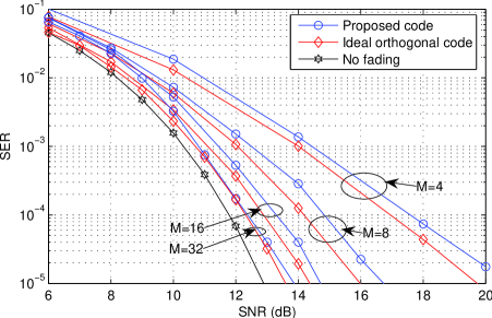
Figure 2: SER versus SNR for various $M$ and $N=1$ with QPSK modulation for the rate-$1$ constructed codes with $M/2$ symbols decoded together and the ideal orthogonal codes.

By using this block diagonal structure, we can construct codes with ML decoding of different symbols together and hence the ML decoding complexity can be controlled. We plot the diversity versus complexity tradeoff in Fig. 1, where $M$ is not necessarily a power of $2$. The code design for such $M$ is done by consturcting a code for $2^{\lceil\log_{2}M\rceil}$ transmit antennas that admits ML decoding complexity of $2^{\lceil\log_{2}M\rceil-n}$ ($n=1,2,\cdots$) and has rank of each partition as $2^{\lceil\log_{2}M\rceil-n+1}$ and then deleting columns suitably chosen to retain the same rank and to have the code matrix of the size $2^{\lceil\log_{2}M\rceil}\times M$.

Note that it is not necessary to assume that $P=M$ i.e. unit rate. One could design codes with $P<M$ that may have additional coding gain while sacrificing code rate.

IV Numerical Results

The symbol error rate (SER) versus the average SNR per receive antenna for the proposed rate-$1$ code that admits decoding in pairs of symbols is plotted in Fig. 2 with QPSK modulation for $M=4,8,16$ and $N=1$. Also plotted is the performance of an ideal rate-$1$ orthogonal space-time codes (non-existent for $M>2$) with equivalent channel as $||H||_{F}$.

Fig. 3 plots the SER curves for $M=16$ and $N=1$ for different ML decoding complexities. Fig. 1 plots the diversity versus complexity tradeoff for the proposed codes.

V Conclusions

We have constructed a class of linear space-time codes that have controllable ML decoding complexity for any number of transmit antennas. The diversity versus decoding complexity tradeoff is shown. We show that one can design rate $1$ codes that achieve performance quite close to the rate $1$ ideal orthogonal codes (non-existent for for $M>2$).

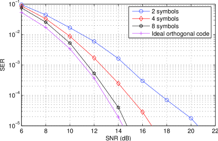
Figure 3: SER versus SNR for $M=16$ and $N=1$ with QPSK modulation for the rate-$1$ constructed and the ideal codes for varying decoding complexity.

References

• [1] V. Tarokh, N. Seshadri and A.R. Calderbank, $``$Space-time codes for high data rate wireless communications : Performance criterion and code construction,$"$ IEEE Trans. Inform. Theory, vol. 44, pp. 744-765, March 1998.
• [2] V. Tarokh, H. Jafarkhani and A.R. Calderbank, $``$Space-time block codes from orthogonal designs,$"$ IEEE Trans. Inform. Theory, vol. 45, pp. 1456-1467, July 1999.
• [3] O. Tirkkonen and A. Hottinen, $``$Square-matrix embeddable space-time block codes for complex signal constellations,$"$ IEEE Trans. Inform. Theory, vol. 48, pp. 384-395, Feb. 2002.
• [4] V.M. DaSilva and E.S. Sousa, $``$Fading-resistant modulation using several transmitter antennas,$"$ IEEE Trans. Commun., vol.45, pp. 1236-1244, Oct. 1997.
• [5] M.O. Damen, K. Abed-Meraim and J.-C. Belfiore, $``$Diagonal algebraic space-time block codes,$"$ IEEE Trans. Inform. Theory, vol. 48, pp. 628-636, March 2002.
• [6] J. Boutros and E. Viterbo, $``$Signal space diversity: A power and band-width efficient diversity technique for the Rayleigh fading channel,$"$ IEEE Trans. Inform. Theory, vol. 44, pp. 1453 V1467, July 1998.
• [7] H. Jafarkhani, $``$A quasi-orthogonal space-time block code,$"$ IEEE Trans. Commun., vol. 49, pp. 1-4, Jan. 2001.
• [8] O. Tirkkonen, A. Boariu and A. Hottinen, $``$Minimal non-orthogonality rate 1 space-time block code for 3+ Tx antennas,$"$ in Proc. IEEE ISSSTA, Parsippany, NJ, Sept. 2000.
• [9] O. Tirkkonen, $``$Optimizing space-time block codes by constellation rotations,$"$ in Proc. Finnish Wireless Commun. Workshop 2001, Oct. 2001.
• [10] C. B. Papadias and G. J. Foschini, $``$Capacity-approaching space-time codes for systems employing four transmitter antennas,$"$ IEEE Trans. on Inform. Theory, vol. 49, pp. 726-732, March 2003.
• [11] N. Sharma and C.B. Papadias, $``$Improved quasi-orthogonal codes through constellation rotation,$"$ IEEE Trans. Commun., vol. 51, pp. 332-335, March 2003.
• [12] N. Sharma and C.B. Papadias, $``$Full-rate full-diversity linear quasi-orthogonal space-time codes for any number of transmit antennas,$"$ Proc. Allerton Conf. Commun. Control Computing, Monticello, IL, Oct. 2003, also in EURASIP J. Applied Signal Processing (Special Issue on Advances in Smart Antennas), vol. 2004, no. 9, pp. 1246-1256, Aug. 2004.
• [13] Z. A. Khan and B. S. Rajan, $``$Single-Symbol Maximum-Likelihood Decodable Linear STBCs,$"$ IEEE Trans. Inform. Theory, vol.52, pp. 2062-2091, May 2006.
• [14] D. Wang and X. Xia, $``$Optimal diversity product rotations for quasi-orthogonal STBC with MPSK symbols,$"$ IEEE Commun. Lett., vol. 9, pp. 420-422, May 2005.
• [15] L. Xian and H. Liu, $``$Optimal rotation angles for quasi-orthogonal space-time codes with PSK modulation,$"$ IEEE Commun. Lett., vol. 9, pp. 676-678, Aug. 2005.