A novel set of rotationally and translationally invariant features for images based on the non-commutative bispectrum

Abstract

We propose a new set of rotationally and translationally invariant features for image or pattern recognition and classification. The new features are cubic polynomials in the pixel intensities and provide a richer representation of the original image than most existing systems of invariants. Our construction is based on the generalization of the concept of bispectrum to the three-dimensional rotation group $\mathrm{SO}(3)$, and a projection of the image onto the sphere.

1 Introduction

The representation of data instances in learning algorithms is subject to the conflicting demands of wanting to incorprate as much information as possible about real world objects, and not wanting to introduce spurious information with no physical meaning. Image recognition is perhaps the most striking example of this phenomenon: clearly, the position and orientation of an object inside a larger image is purely a matter of representation and not a property of the object itself.

There have been many attempts to construct rotation and translation invariant representations both in the vision community and in the machine learning world. A faithful representation of invariances is particularly important when pushing algorithms towards the limit of small training sets. When training data is abundant, it can drone out spurious degrees of freedom or average over them. However, in small datasets effective generalization is not possible without explicitly taking the invariances into account.

Various types of invariants are used in signal processing and computer vison, each with its own advantages and disadvantages (see, e.g., [9][7]). However, a common feature of most of these invariants is that they are lossy, in the sense that they do not uniquely specify the original data image. This becomes a particularly serious problem in discriminative learning, where the success of modern algorithms is to a large extent based on their ability to handle very high dimensional data, capturing as much information about data instances as possible. This is why in many cases (such as the character recognition problem to be addressed in the experimental section) it has often proven to be better to ignore the invariance altogether rather than risk losing valuable information as a side-effect of enforcing it.

Another potential problem with existing methods is their high computational cost. Approaches based on summing over members of the invariance group (ghost instances, etc.) and methods that require an expensive kernel evaluation for each pair of instances suffer specially badly from speed issues (e.g., [5]).

In this paper we propose a new class of invariant features for two dimensional images based on the algebra of generalized bispectra and a projection from the image plane onto the sphere. The new invariant features are strictly rotation and translation invariant (up to our bandwidth restriction and a small projection error), and close to complete, in the sense of uniquely specifying the original image up to a single rotation and translation. The bispectral invariants can be computed in a pre-processing step before any learning takes place in time $O(u^{5/2})$, where $u$ is the size of the original image in pixels. The individual invariants are third order polynomials in the pixel intensities, and hence are relatively well behaved. We envisage the invariants to be used as inputs to an existing machine learning algorithm, for example as features to build kernels from. Our experiments show that using the bispectral invariants makes an immediate impact on a standard optical character recognition task when the training and testing intances are allowed to randomly translate and rotate.

While the bispectrum is well known in some areas of vision and signal processing, most practicioners are only familiar with its classical “Euclidean” version [2]. For our purposes this is not sufficient because rotations and translations together form a non-commutative group. In particular, previous work on using the bispectrum for translation and rotation invariance considered these two types of transformations separately, first eliminating the unknown translation and then the rotation from the image [8]. While this is possible for image reconstruction, as regards generating invariant features it would amount to no more than transforming the image to a canonical position and orientation, which is obviosuly sensitive to variations in the image, since small changes can lead to vastly different optimal alignments with the canonical orientation.

While there is a well-developed and beautiful abstract theory of bispectra on general compact groups developed chiefly by Ramakrishna Kakarala [4] [3] [1], not many connections of the non-commutative case to real world problems have been explored. To the best of our knowledge, bispectra over non-commutative groups have never been used in the context of simultaneously enforcing rotational and translational symmetries of two-dimensional images. The crucial new device connecting rotations and translations of the plane to the action of a compact non-commutative group is the projection onto the sphere proposed in this paper.

The first half of this paper sets the scene by giving a rather abstract and general introduction to the theory of bispectra on groups. The second half of the paper contains our actual construction and the details of implementing it on a computer. The reader who is not interested in the wider context of bispectral invariants might find it convenient to skip directly to section 3.

2 Bispectral Invariants

The discrete Fourier transform of a complex-valued function $f\colon\left\{0,1,2,\ldots,n-1\right\}\to\mathbb{C}$ is defined

$$\widehat{f}(k)=\sum_{x=0}^{n-1}e^{-i2\pi xk/n}\>f(x),$$ (1)

where $k$ extends over $0,1,2,\ldots,n-1$ and each component $\widehat{f}(k)$ is the coefficient of the contribution to $f$ at frequency $k$. A natural quantity of interest in signal processing is then the power spectrum

$$q(k)={\widehat{f}^{\ast}(k)}\cdot\widehat{f}(k),$$ (2)

where ^∗ denotes complex conjugation. The power spectrum quantifies how much energy the signal has in each frequency band. Intuitively it is clear that the power spectrum should be invariant to translations of the signal. This is also borne out by the fact that by the convolution theorem the power spectrum is the Fourier transform of the autocorrelation function

$$\mathrm{corr}(x)=\sum_{y=0}^{n-1}f(y+x)\,{f^{\ast}(y)},$$ (3)

(Wiener-Khinchin theorem) which is manifestly shift-invariant. Here and in the following addition and subtraction of indices and frequencies in $\left\{0,1,2,\ldots,n-1\right\}$ is always to be understood modulo $n$.

More formally, we define the translate of $f$ by $z$ as $f^{z}(x)=f(x-z)$. Plugging into (1),

$$\widehat{f}^{z}(k)=\sum_{x=0}^{n-1}e^{-i2\pi xk/n}\>f(x-z)=\\ \sum_{x=0}^{n-1}e^{-i2\pi(x+z)k/n}\>f(x)=e^{-i2\pi zk/n}\widehat{f}(k),\\$$ (4)

which shows that under translation each component of $\widehat{f}$ is simply premultiplied by an $e^{-i2\pi zk/n}$ factor.

The invariance of the spectrum is the result of the fact that in (2) these factors cancel:

$$q^{z}(k)=\bigl{(}e^{-i2\pi zk/n}\,\widehat{f}(k)\bigr{)}^{\ast}\cdot\bigl{(}e^{-i2\pi zk/n}\,f(k)\bigr{)}=\\ e^{i2\pi zk/n}\,{\widehat{f}^{\ast}(k)}\,e^{-i2\pi zk/n}\,f(k)={\widehat{f}^{\ast}(k)}\cdot f(k)=q(k).$$

The spectrum is often used in signal processing applications as a translation invariant characterization of functions. Unforunately, in computing the spectrum we lose all phase information: the spectrum only measures the energy in each band, not its phase relative to other bands.

The idea behind bispectral invariants is to move from (3) to the triple correlation

$$a(x_{1},x_{2})=\sum_{y=0}^{n-1}{f^{\ast}(y-x_{1})}\>{f^{\ast}(y-x_{2})}\,f(y).$$

Note that in some of the literature the triple correlation is defined slightly differently, and the above quantity would be ${a^{\ast}(-x_{1},-x_{2})}$. We deviate from this convention so as to make the formulae involved in the generalization to groups slightly more transparent. Again by the convolution theorem, the (2-dimensional) Fourier transform of this function is

$$b(k_{1},k_{2})={\widehat{f}^{\ast}(k_{1})}\>{\widehat{f}^{\ast}(k_{2})}\,\widehat{f}(k_{1}+k_{2}),$$

and this is what is called the bispectrum of $f$. Under translation $b$ becomes

$$b^{z}(k_{1},k_{2})=e^{i2\pi zk_{1}/n}{\widehat{f}^{\ast}(k_{1})}\cdot e^{i2\pi zk_{2}/n}{\widehat{f}^{\ast}(k_{2})}\>\cdot\\ e^{-i2\pi z(k_{1}+k_{2})/n}\>\widehat{f}(k_{1}+k_{2})=b(k_{1},k_{2}),$$

so the bispectrum is invariant. The remarkable fact is that unlike the ordinary power spectrum, $b$ is also sufficient to reconstruct the original signal up to translation. The bispectrum is widely used in signal processing as a lossless shift-invariant representation, and various algorithms have been devised to reconstruct $f$ from $b$.

2.1 Bispectrum on groups

The “Euclidean” bispectrum introduced above would already be sufficient to construct translation invariant kernels. However, if we are to construct a kernel which is invariant to both translation and rotation, due to the intricate way in which these operations interact, we need to take a slightly more abstract viewpoint and re-examine what was said above from the point of view of group theory. While the concept of “Euclidean” bispectra is fairly well known in signal processing and computer vision, its generalization to non-commutative groups has attracted much less attention. The pioneering researcher in this field was R. Kakarala [3].

Recall that a group $G$ is a set with a multiplication operation $\cdot\>\colon G\times G\to G$ obeying the following axioms:

1. For any $x,y\in G$,  $xy\in G$ (closure);

2. For any $x,y,z\in G$,  $({xy})z=x({yz})$ (associativity);

3. There is a unique element of $G$ denoted $e$ and called the identity for which $ex=xe=x$ for any $x\in G$;

4. For any $x\in G$ there is a corresponding element $x^{-1}\in G$ called the inverse of $x$, which satisfies $xx^{-1}=x^{-1}x=e$ for any $x\in G$.

Significantly, groups need not be commutative, i.e., $xy$ need not equal $yx$. This is crucial for our present purposes since rigid planar motions don’t commute.

Given a group $G$ and a function $f\colon G\to\mathbb{C}$ to define the Fourier transform of $f$ we need to introduce the concept of group representations. A representation is essentially a way of modeling the group operation by the multiplication of complex valued matrices. We say that $\rho\colon G\to\mathbb{C}^{d_{\rho}\times d_{\rho}}$ is a representation of $G$ if

$$\rho(xy)=\rho(x)\hskip 1.11115pt\rho(y)$$

for any $x,y\in G$. We also require $\rho(e)=I$. We say that $d_{\rho}$ is the dimensionality of the representation. Note that $\rho(x^{-1})=\left(\rho(x)\right)^{-1}$.

There are some trivial ways of producing new representations from existing ones. For example, if $\rho_{1}$ is a representation of $G$, then for any invertible matrix $T$, so is $T^{-1}\rho_{1}(x)\,T$. These representations are clearly not substantially different, so they are called equivalent.

Another way that representations may be related is when a larger representation splits into smaller ones. We say that $\rho$ is reducible if some invertible square matrix $T$ can block diagonalize it in the form

$$T^{-1}\rho(x)\,T=\left(\begin{array}[]{c|c}\rho_{1}(x)&0\\ \hline\cr 0&\rho_{2}(x)\end{array}\right)\qquad\quad x\in G$$

into a direct sum of smaller representations $\rho_{1}$ and $\rho_{2}$.

To develop the theory what are really important are the irreducible representations that cannot be reduced in this way. Given a group $G$ there is a lot of interest in constructing a complete set of inequivalent representations for it. Such a set we will denote by $\mathcal{R}$. For a wide range of groups we can choose $\mathcal{R}$ to consist exclusively of unitary representations, so from now on we assume that $\rho(x^{-1})=\rho(x)^{\dagger}$, where ^† denotes the conjugate transpose.

With these concepts of representation theory in hand, we return to (1) and note that the exponential factors appearing in the summation are nothing but representations (specifically, one-dimensional, irreducible representations) of the group formed by $\left\{0,1,2,\ldots,n-1\right\}$ with respect to addition modulo $n$. This suggests generalizing Fourier transformation to the non-commutative realm in the form

$$\widehat{f}(\rho)=\sum_{x\in G}f(x)\hskip 1.11115pt\rho(x)\qquad\quad\rho\in\mathcal{R}.$$ (5)

Here and in the following the summation sign either denotes a discrete sum over the elements of a discrete group, or an integral (with respect to Haar measure) over a Lie group. Note that in contrast to (1), for general groups the components of $\widehat{f}$ are matrices and not scalars, and they are not indexed by the elments of $G$, but by its irreducible representations.

The generalized Fourier transform shares many important properties with its Euclidean counterpart, but most of these will not concern us here. What is important is that there is a natural concept of translation of functions on $G$ defined by

$$f^{z}(x)=f(z^{-1}x)\qquad\quad z\in G,$$

and that by the defining property of representations,

$$\widehat{f}^{z}(\rho)=\sum_{x\in G}f(z^{-1}x)\hskip 1.11115pt\rho(x)=\\ \sum_{x\in G}f(z^{-1}x)\hskip 1.11115pt\rho(z)\rho(z^{-1}x)=\\ \rho(z)\sum_{x\in G}f(x)\hskip 1.11115pt\rho(x)=\rho(z)\widehat{f}(\rho)$$

in exact analogy with (4). In particular, by the unitarity of $\rho$, the generalized power spectrum $q(\rho)=\widehat{f}(\rho)^{\dagger}\widehat{f}(\rho)$ is again invariant to translation:

$$q^{z}(\rho)=\bigl{(}\rho(z)\widehat{f}(\rho)\bigr{)}^{\dagger}\bigl{(}\rho(z)\widehat{f}(\rho)\bigr{)}=\\ f(\rho)^{\dagger}\rho(z)^{\dagger}\rho(z)f(\rho)^{\dagger}=\widehat{f}(\rho)^{\dagger}\widehat{f}(\rho).$$

As in the classical case, the power spectrum does not uniquely determine $f$. The loss of information is related to the fact that the $q(\rho)$ matrices are by definition constrained to be positive definite, and again the power spectrum is insensitive to phase information in the sense that we may multiply any Fourier component by a different invertible matrix without affecting the power spectrum.

To construct the bispectrum we need to couple the different components of $\widehat{f}$, while at the same time retaining invariance. Consider tensor products $\widehat{f}(\rho_{1})\otimes\widehat{f}(\rho_{2})$, which transform according to

$$\widehat{f}^{z}(\rho_{1})\otimes\widehat{f}^{z}(\rho_{2})=\left(\rho_{1}(z)\otimes\rho_{2}(z)\right)\bigl{(}\widehat{f}(\rho_{1})\otimes\widehat{f}(\rho_{2})\bigr{)}.$$

Now $\rho_{1}(z)\otimes\rho_{2}(z)$ is also a representation of $G$, but typically it is not irreducible. However, for wide classes of groups tensor product representations decompose into irreducibles in the form

$$\rho_{1}(z)\otimes\rho_{2}(z)=C\>\Bigl{[}\bigoplus_{\rho}\rho(z)\Bigr{]}\>C^{\dagger}.$$

Determining which set of irreducibles the direct sum ranges over (and with what multiplicities) and what the unitary matrix $C$ should be is in general a highly non-trivial problem in representation theory. For now we assume that this so-called Clebsch-Gordan decomposition is known.

In this case we have a generalized bispectrum

$$b(\rho_{1},\rho_{2})=C^{\dagger}\>\bigl{(}\widehat{f}(\rho_{1})\otimes\widehat{f}(\rho_{2})\bigr{)}^{\dagger}\>C\>\bigoplus_{\rho}\>\widehat{f}(\rho),$$ (6)

and it will be translation invariant, $b^{z}(\rho_{1},\rho_{2})=b(\rho_{1},\rho_{2})$. What goes beyond a straightforward generalization of the classical results is the proof that for a wide range of groups, including all compact groups, if all $\widehat{f}(\rho)$ Fourier components are invertible matrices, then $b$ uniquely determines $f$ up to translation. This is a highly technical result proved in [3], and in constrast to the commutative case, there might not be an algorithm for recovering $f$.

2.2 Homogeneous spaces

Before addressing the problem of image invariants, we need one more technical extension of the foregoing. We say that a group $G$ acts on a space $X$, if for any $g\in G$ there is a mapping $T_{g}\colon X\to X$ such that if $g_{2}g_{1}=g_{3}$, then $T_{g_{1}}(T_{g_{2}}(x))=T_{g_{3}}(x)$ for any $x\in X$. Now $X$ is a homogeneous space of $G$ if fixing any $x_{0}\in X$, the set $T_{g}(x_{0})$ ranges over the whole of $X$ as $g$ ranges over $G$. The classical example of a homogenous space, which will also be our choice for our image recognition problem, is the unit sphere $S_{2}$. The sphere is a homogeneous space of the three-dimensional rotation group $\mathrm{SO}(3)$: taking the North pole as $x_{0}$, a suitable rotation can move it to any point $x\in S_{2}$.

Fourier transformation generalizes naturally to functions $f\colon X\to\mathbb{C}$:

$$\widehat{f}(\rho)=\sum_{g\in G}f(T_{g}(x_{0}))\hskip 1.11115pt\rho(g)\qquad\quad\rho\in\mathcal{R},$$

as does the concept of translation, $f^{g}(x)=f(T_{g^{-1}}(x))$, and the bispectrum (6) remains invariant to such translations.

Note that except for the trivial case $X=G$, Fourier transforms on homogeneous spaces are naturally redundant: typically $X$ is a much smaller space than $G$, yet a Fourier transform on $X$ has the same number of components as a Fourier transform on the entire group. One manifestation of this fact is that we might find that some Fourier components are rank deficient no matter what $f\colon X\to\mathbb{C}$ we choose. While this destroys Kakarala’s uniqueness result, in practice we often find that the bispectrum still furnishes a remarkably rich invariant representation of $f$. We remark that that invariance to right-translation $f^{(z)}(x)=f(xz^{-1})$ would be a different matter: there is a variant of the bispectrum which retains the uniqueness property in this case (Theorem 3.3.6 in [3]).

3 Bispectral invariants for images

After the abstract discussion of the previous section we now set out to construct concrete invariants for 2D monochrome images. We represent an image as an intensity function $h\colon\mathbb{R}^{2}\to\left[0,1\right]$ with support confined to a compact region of the plane, for example, the square $\left[-0.5,0.5\right]^{2}$. The group that we would ideally like to be working with encompassing all translations and rotations is the Euclidean group $\mathrm{ISO}^{+}\!\hskip 0.55557pt(2)$ of rigid body motions in the plane. $\mathbb{R}^{2}$ is a homogeneous space of $\mathrm{ISO}^{+}\!\hskip 0.55557pt(2)$, so we could compute the $\mathrm{ISO}^{+}\!\hskip 0.55557pt(2)$-Fourier transform of our image, and construct its bispectrum as described above.

The problem with this approach is that $\mathrm{ISO}^{+}\!\hskip 0.55557pt(2)$ is not compact. Although it does belong to a class of exceptional groups to which Kakarala’s uniqueness result does apply, its representation theory is complicated and computing the bispectrum is likely to be computationally very challenging. The main contribution of this paper is to show how the reduce the problem to rotations of the sphere. The rotation group $\mathrm{SO}(3)$ also happens to have the simplest and best known non-trivial Clebsch-Gordan decomposition. To make the exposition as elementary as possible, we derive the bispectral invariants from first principles, exploiting the simplifications afforded by this special case.

3.1 Projection onto the sphere

We begin by projecting our image $h$ onto the unit sphere $S_{2}$. The simplest possible projection is to project parallel to the $z$-axis, formally

$$h\mapsto f,\qquad f(\theta,\phi)=h(r_{\mathbb{R}^{2}},\theta_{\mathbb{R}^{2}})=h({\textstyle\frac{1}{a}}\theta,\phi),$$ (7)

where $0\leq\theta\leq\pi$ and $0\leq\phi<2\pi$ are spherical polar coordinates, while $r_{\mathbb{R}^{2}}=\frac{1}{a}\theta$ and $\theta_{\mathbb{R}^{2}}=\phi$ are planar polars. The magnification parameter $a$ we are free to choose between reasonable bounds as long as our image “fits” on the surface of the sphere. Inevitably, such a mapping does involve some distortion, particulary at the corners, as the image conforms to the curved surface of $S_{2}$. Reducing $a$ decreases this distortion at the expense of reducing the surface area of the sphere actually occupied by the image, and hence increasing the computaional cost at the same effective resolution. In practice, even relatively large values of $a$ (up to $1.5$) do not hurt performance. Apart from the inevitable finite bandwidth cutoff, this is the only approximation involved in our method.

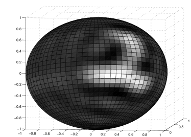
Figure 1: A NIST handwritten digit projected onto the sphere. The band-limit is $L=15$. Note that there is a minimal amount of “ringing”.

To numerically represent $f$ we use spherical harmonics

$$Y_{l}^{m}(\theta,\phi)=\sqrt{\frac{2l+1}{4\pi}\frac{\left(l-m\right)!}{\left(l+m\right)!}}~{}~{}P_{l}^{m}(\cos\theta)~{}e^{im\phi},$$

where $l=0,1,2,\ldots$;  $m=-l,-l+1,\ldots,l$ and $P_{l}^{m}$ are the associated Legendre polynomials. Recall that the spherical harmonics are the eignefunctions of the Laplace operator on $S_{2}$ (with eigenvalue $-l^{2}$), and they form an orthonormal basis for $L_{2}(S_{2})$, thus we can represent $f$ as

$$f(\theta,\phi)=\sum_{l=0}^{\infty}\sum_{m=-l}^{l}\widehat{f}_{l,m}\,Y_{l}^{m}(\theta,\phi)\qquad\quad$$ (8)

where $\widehat{f}_{l,m}=\left\langle f,Y_{l}^{m}\right\rangle$ and $\left\langle\cdot,\cdot\right\rangle$ is the inner product

$$\left\langle f,g\right\rangle=\int_{0}^{\pi}\int_{0}^{2\pi}{f^{\ast}(\theta,\phi)}\,g(\theta,\phi)\cos\theta\>d\phi\>d\theta.$$

We denote by $\mbox{\boldmath$\widehat{f}$}_{l}$ the vector $(\widehat{f}_{l,-l},\widehat{f}_{l,-l+1},\ldots,\widehat{f}_{l,l})$.

Viewing $S_{2}$ as a homogeneous space of $\mathrm{SO}(3)$, the $\{\widehat{f}_{l,m}\}$ are the Fourier coefficients of $f\colon S_{2}\to\mathbb{C}$ as defined in the previous section. However, in this special case they do not form matrices, only vectors: if we formally computed (2.2), we would find that only the first column of each matrix is non-zero (see also [1]). This will make the computational burden significantly lighter.

In a computational setting we must truncate (8) at some finite $L$, preferably so as to match the resolution of our original image. In general, the spherical representation of an image requires more storage than the original pixmap representation only to the extent that the image only occupies a fraction of the surface of the sphere.

For a $\left[0,1\right]$-valued bitmap matrix M, the mapping (7) leads to

$$\widehat{f}_{l,m}=\sum_{i,j=1}^{n}M_{i,j}Y_{l}^{m}(\theta,\phi),$$ (9)

where $\theta=a\sqrt{x^{2}+y^{2}}$,

$$\phi=\begin{cases}~{}\arctan(y/x)&\text{if~{}~{}}y>0\\ ~{}2\pi-\arctan(y/x)&\text{if~{}~{}}y<0\\ \end{cases},$$

and $\left(x,y\right)=\bigl{(}\,\frac{i-1/2}{N}-0.5,~{}\frac{j-1/2}{N}-0.5\bigr{)}$.

Just as the isometry group of $\mathbb{R}^{2}$ is $\mathrm{ISO}^{+}(2)$, the isometry group of $S_{2}$ is $\mathrm{SO}(3)$, the group of rotations of $\mathbb{R}^{3}$ about the origin. It is easy to visualize that given the mapping (7), locally, around the north pole, there is a one-to one corresponence between the action of $\mathrm{SO}(3)$ on functions on the sphere and of $\mathrm{ISO}^{+}(2)$ on the corresponding functions on the plane. In other words, any rigid motion of an image in the plane can be imitated by a 3D rotation of the corresponding function on $S_{2}$. Rotations of the image around the center of the image correspond to rotations of the sphere about the $z$ axis (pole to pole), while translations correspond to rotations around the $x$ and $y$ axes. Exploiting this fact, we proceed by computing the bispectral invariants of $f$ with respect to $\mathrm{SO}(3)$ and let these be our translation and rotation invariant features.

3.2 An $\mathrm{SO}(3)$-invariant kernel on $L_{2}(S_{2})$

To construct the $\mathrm{SO}(3)$-invariant features, we examine how $\mathrm{SO}(3)$ acts on individual spherical harmonics. Since $\left\{Y_{l}^{m}\right\}_{m=-l,\ldots,l}$ span the space of eigenvectors of the Laplace operator with eigenvalue $-l^{2}$, and since the Laplace operator is rotationally invariant, under the action of a rotation $R\in\mathrm{SO}(3)$,  $Y_{l}^{m}$ must transform into a linear combination $R(Y_{l}^{m})=\sum_{m^{\prime}=-l}^{l}a_{m}Y_{l}^{m^{\prime}}$ of other spherical harmonics of the same order $l$.

For a general function $f\in L_{2}(S_{2})$, under a rotation $R\in\mathrm{SO}(3)$ the Fourier coefficients transform according to

$$\left(\begin{matrix}\widehat{f}_{l,-l}^{\prime}\\ \vdots\\ \widehat{f}_{l,l}^{\prime}\end{matrix}\right)=D^{(l)}(R)\left(\begin{matrix}\widehat{f}_{l,-l}\\ \vdots\\ \widehat{f}_{l,l}\end{matrix}\right),$$ (10)

where $D^{(l)}(R)$ are $(2l+1)\times(2l+1)$ dimensional matrices. In fact, $D^{(0)},D^{(1)},\ldots$ are exactly the (complex-valued) irreducible representations of $\mathrm{SO}(3)$.

Figure 2: The inner product matrix between the bispectrum representation of the ”0” and ”1” digits from the first 300 translated and rotated NIST characters. The block structure reflects that the intra-class inner products are higher than the inter-class products.

It is possible to show that the $D^{(l)}$ are unitary representations, hence the polynomials

$$p_{l}=\sum_{m=-l}^{l}\bigl{|}\,\widehat{f}_{l,m}\,\bigr{|}^{2}=\mbox{\boldmath$\widehat{f}$}_{l}^{\dagger}\cdot\mbox{\boldmath$\widehat{f}$}_{l}=\left(\begin{matrix}\widehat{f}_{l,-l}^{\ast},\ldots,\widehat{f}_{l,l}^{\ast}\end{matrix}\right)\cdot\left(\begin{matrix}\widehat{f}_{l,-l}\\ \vdots\\ \widehat{f}_{l,l}\end{matrix}\right)$$

transform according to

$$p_{l}\mapsto\bigl{(}D^{(l)}(R)\,\mbox{\boldmath$\widehat{f}$}_{l}\bigr{)}^{\dagger}\cdot\bigl{(}D^{(l)}(R)\,\mbox{\boldmath$\widehat{f}$}_{l}\bigr{)}=\\ \mbox{\boldmath$\widehat{f}$}_{l}^{\dagger}\,(D^{(l)}(R))^{\dagger}\,(D^{(l)}(R))\,\mbox{\boldmath$\widehat{f}$}_{l}=\mbox{\boldmath$\widehat{f}$}_{l}^{\dagger}\cdot\mbox{\boldmath$\widehat{f}$}_{l},$$

i.e., they are invariant. This is the power spectrum, as defined in Section 2.1. As before, this is an invariant, but very impoverished representation of $f$.

Figure 3: The first few rotated and translated NIST characters.

The bispectrum is derived by considering the $(2l_{1}+1)(2l_{2}+1)$-dimensional tensor product vectors $\mbox{\boldmath$\widehat{f}$}_{l_{1}}\otimes\mbox{\boldmath$\widehat{f}$}_{l_{2}}$, which transform according to

$$\mbox{\boldmath$\widehat{f}$}_{l_{1}}\otimes\mbox{\boldmath$\widehat{f}$}_{l_{2}}\mapsto\bigl{(}D^{(l_{1})}(R)\otimes D^{(l_{2})}(R)\bigr{)}\cdot\bigl{(}\mbox{\boldmath$\widehat{f}$}_{l_{1}}\otimes\mbox{\boldmath$\widehat{f}$}_{l_{2}}\bigr{)}.$$ (11)

The representation theory of $\mathrm{SO}(3)$ is well developed, in particular, it is well known that the tensor product representations decompose in the form

$$D^{(l_{1})}(R)\otimes D^{(l_{2})}(R)=\\ \left(C^{l_{1},l_{2}}\right)^{\dagger}\biggl{[}~{}\bigoplus_{l=\left|\,l_{1}-l_{2}\,\right|}^{l_{1}+l_{2}}D^{(l)}(R)~{}\biggr{]}\;C^{l_{1},l_{2}}.$$

Here ${C^{l_{1},l_{2}}}$ is a $((2l_{1}+1)(2l_{2}+1))\times((2l_{1}+1)(2l_{2}+1))$-element unitary matrix, with rows labeled by the pair $\left(l,m\right)$ and columns labeled by the pair $\left(m_{1},m_{2}\right)$. The matrix elements $C^{l_{1},l_{2},l}_{m_{1},m_{2},m}=\left[C^{l_{1},l_{2}}\right]_{(l,m),(m_{1},m_{2})}$ are called Clebsch-Gordan coefficients, and are implemented in most computational algebra packages. Our notation is redundant in that it is possible to show that $C^{l_{1},l_{2},l}_{m_{1},m_{2},m}$ vanishes unless $m_{1}+m_{2}=m$, hence we only need to worry about the coefficients $C^{l_{1},l_{2},l}_{m_{1},m-m_{1},m}$.

Thus, under rotation $C^{l_{1},l_{2}}\bigl{(}\mbox{\boldmath$\widehat{f}$}_{l_{1}}\otimes\mbox{\boldmath$\widehat{f}$}_{l_{2}}\bigr{)}$ transforms according to

$$C^{l_{1},l_{2}}\bigl{(}\mbox{\boldmath$\widehat{f}$}_{l_{1}}\otimes\mbox{\boldmath$\widehat{f}$}_{l_{2}}\bigr{)}\mapsto\biggl{[}~{}\bigoplus_{l=\left|\,l_{1}-l_{2}\,\right|}^{l_{1}+l_{2}}D^{(l)}(R)~{}\biggr{]}\;C^{l_{1},l_{2}}\>\bigl{(}\mbox{\boldmath$\widehat{f}$}_{l_{1}}\otimes\mbox{\boldmath$\widehat{f}$}_{l_{2}}\bigr{)}.$$ (12)

Writing $C^{l_{1},l_{2}}\bigl{(}\mbox{\boldmath$\widehat{f}$}_{l_{1}}\otimes\mbox{\boldmath$\widehat{f}$}_{l_{2}}\bigr{)}=\bigoplus_{l=\left|\,l_{1}-l_{2}\,\right|}^{l_{1}+l_{2}}\widehat{\mbox{\boldmath$g$}}_{l_{1},l_{2},l}$, where

$$\left[\,\widehat{\mbox{\boldmath$g$}}_{l_{1},l_{2},l}\,\right]_{m}=\sum_{m_{1}=-l_{1}}^{l_{1}}C^{l_{1},l_{2},l}_{m_{1},m-m_{1},m}\,\widehat{f}_{l_{1},m_{1}}\,\widehat{f}_{l_{2},m-m_{1}},$$

$\widehat{\mbox{\boldmath$g$}}_{l_{1},l_{2},l}$ transforms according to

$${\widehat{\mbox{\boldmath$g$}}_{l_{1},l_{2},l}\mapsto D^{(l)}(R)\,\widehat{\mbox{\boldmath$g$}}_{l_{1},l_{2},l}}.$$

By the same argument as for the power spectrum, this gives rise to the cubic invariants

$$p_{l_{1},l_{2},l}=\widehat{\mbox{\boldmath$g$}}_{l_{1},l_{2},l}^{\dagger}\cdot\widehat{\mbox{\boldmath$f$}}_{l}=\\ \sum_{m=-l}^{l}\sum_{m_{1}=-l_{1}}^{l_{1}}C^{l_{1},l_{2},l}_{m_{1},m-m_{1},m}\,\widehat{f}_{l_{1},m_{1}}^{\ast}\,\widehat{f}_{l_{2},m-m_{1}}^{\ast}\,\widehat{f}_{l,m}.$$ (13)

Up to unitary transformation, these invariants are equivalent to the non-vanishing matrix elements of the abstract bispectrum (as already derived in [3] and [1]). Any kernel built from the bispectrum using (13) as features will be invariant to translation and rotation.

3.3 Computational considerations

	1	2	3	4	5	6	7	8	9
0	${0.77(0.41)}$	${6.22(2.41)}$	${5.09(1.54)}$	${5.03(1.07)}$	${2.90(1.53)}$	${4.11(2.39)}$	${2.73(1.11)}$	${4.98(1.64)}$	${5.86(2.88)}$
	${17.12(3.67)}$	${33.87(3.59)}$	${42.06(3.59)}$	${30.64(2.53)}$	${37.82(3.51)}$	${31.42(5.85)}$	${29.36(3.83)}$	${42.58(4.33)}$	${27.61(3.16)}$
1		${0.68(0.81)}$	${0.39(0.98)}$	${3.07(1.30)}$	${0.00(0.00)}$	${1.37(0.88)}$	${1.77(1.48)}$	${2.68(2.02)}$	${1.02(1.00)}$
		${30.78(2.90)}$	${29.34(4.50)}$	${34.96(3.41)}$	${30.66(2.85)}$	${34.46(4.47)}$	${38.32(4.05)}$	${24.60(2.57)}$	${34.78(3.57)}$
2			${15.89(5.79)}$	${15.82(3.22)}$	${8.06(3.60)}$	${9.64(2.00)}$	${11.11(2.29)}$	${9.26(1.63)}$	${10.55(2.95)}$
			${49.06(4.18)}$	${47.12(4.72)}$	${45.20(4.26)}$	${51.44(5.21)}$	${47.20(5.54)}$	${47.44(6.23)}$	${46.70(2.95)}$
3				${4.81(1.68)}$	${16.42(5.69)}$	${7.54(2.75)}$	${4.00(1.13)}$	${10.70(3.79)}$	${7.66(3.01)}$
				${44.64(3.03)}$	${49.07(4.81)}$	${49.38(5.26)}$	${44.74(4.42)}$	${50.37(4.21)}$	${47.60(5.55)}$
4					${6.26(1.90)}$	${10.94(4.09)}$	${14.95(2.89)}$	${6.27(3.57)}$	${16.95(1.84)}$
					${40.08(6.67)}$	${50.11(5.26)}$	${45.30(3.30)}$	${46.26(2.63)}$	${49.82(4.68)}$
5						${14.63(2.42)}$	${5.31(2.27)}$	${6.62(2.72)}$	${6.84(2.23)}$
						${50.00(4.02)}$	${41.70(4.09)}$	${44.63(3.31)}$	${46.01(4.37)}$
6							${7.68(4.05)}$	${9.00(2.93)}$	${20.15(3.62)}$
							${48.19(4.10)}$	${46.13(5.82)}$	${53.75(2.69)}$
7								${3.50(2.28)}$	${8.06(3.49)}$
								${41.16(5.18)}$	${53.21(5.01)}$
8									${9.43(2.14)}$
									${45.13(2.87)}$

Table 1: Classification error in percent for each pair of digits for the linear kernels. The performance of the bispectrum-based classifier is shown on top, and the baseline on bottom; standard errors are in parentheses.

The algorithmic implementation of (13) is

$$p_{l_{1},l_{2},l}=\sum_{m=-l}^{l}\widehat{f}_{l,m}\times\\ \times\sum_{m_{1}=\max(-l_{1},m-l_{2})}^{\min(l_{1},m+l_{2})}C^{l_{1},l_{2},l}_{m_{1},m-m_{1},m}\,\widehat{f}_{l_{1},m_{1}}^{\ast}\,{\widehat{f}_{l_{2},m-m_{1}}^{\ast}},$$

which gives $O(L^{3})$ invariant features to build the kernel from. The features can be precomputed as a data processing step before any learning actually takes place. Typically, $L$ will scale linearly with the linear dimension $w$ of the input image in pixels, so the bispectrum inflates the data at a rate of $u^{3/2}$, where $u$ is the original storage size of a single image.

Projecting onto the sphere is a linear map and its coefficients can be precomputed, so the cost of that operations scales with $w^{2}L^{2}\propto u^{2}$. Finally, computing the bispectrum itself scales with $L^{5}\propto u^{5/2}$. On the desktop PC used to prepare the data for the experiments, processing each $30\times 30$ pixel image took approximately 100ms for $L=15$.

	1	2	3	4	5	6	7	8	9
0	${0.80(0.42)}$	${5.06(1.52)}$	${4.78(1.08)}$	${3.35(1.69)}$	${3.90(2.25)}$	${3.07(1.77)}$	${4.48(1.39)}$	${3.74(2.23)}$	${6.34(2.57)}$
	${12.50(3.60)}$	${26.30(4.32)}$	${33.72(4.58)}$	${32.45(12.63)}$	${29.52(3.99)}$	${23.51(4.93)}$	${24.96(3.73)}$	${29.99(4.20)}$	${19.16(2.65)}$
1		${0.99(0.48)}$	${0.00(0.00)}$	${2.48(0.97)}$	${0.21(0.45)}$	${1.35(0.43)}$	${1.22(1.09)}$	${0.52(0.55)}$	${3.05(0.88)}$
		${27.29(4.00)}$	${22.61(8.82)}$	${33.98(9.44)}$	${30.86(9.99)}$	${28.52(9.47)}$	${32.12(6.34)}$	${20.16(2.93)}$	${28.01(4.56)}$
2			${14.68(4.60)}$	${13.20(2.56)}$	${8.83(4.22)}$	${8.89(3.09)}$	${12.73(3.39)}$	${12.14(2.27)}$	${10.34(2.51)}$
			${47.75(3.46)}$	${45.26(5.11)}$	${50.09(4.78)}$	${45.63(5.49)}$	${43.84(4.38)}$	${44.02(3.14)}$	${45.95(4.84)}$
3				${5.12(2.35)}$	${16.88(2.73)}$	${6.98(3.46)}$	${3.50(1.48)}$	${10.21(3.89)}$	${5.08(1.50)}$
				${43.07(9.05)}$	${52.53(3.39)}$	${45.86(5.27)}$	${41.90(4.09)}$	${46.00(4.97)}$	${44.87(3.91)}$
4					${5.75(1.22)}$	${10.67(1.47)}$	${13.92(2.63)}$	${6.45(2.26)}$	${12.09(2.47)}$
					${39.21(4.29)}$	${46.82(5.32)}$	${46.73(6.47)}$	${42.29(4.44)}$	${52.73(3.65)}$
5						${16.56(1.66)}$	${6.26(1.54)}$	${6.23(3.05)}$	${7.07(2.93)}$
						${47.04(4.21)}$	${46.39(3.41)}$	${41.63(3.29)}$	${43.23(2.46)}$
6							${9.30(3.33)}$	${6.16(2.30)}$	${21.37(3.81)}$
							${40.43(5.16)}$	${41.19(4.47)}$	${50.73(4.31)}$
7								${4.68(2.30)}$	${8.81(2.81)}$
								${37.33(2.21)}$	${46.22(4.13)}$
8									${10.06(2.04)}$
									${44.06(3.93)}$

Table 2: Classification error in percent for each pair of digits for the Gaussian RBF kernels. The performance of the bispectrum-based classifier is shown on top, and the baseline on bottom, standard errors are in parentheses.

4 Experiments

We conducted experiments on randomly translated and rotated versions of hand-written digits from the well known NIST dataset [6]. The original images are size $28\times 28$, but most of them only occupy a fraction of the image patch. The characters are rotated by a random angle between $0$ and $2\pi$, clipped, and embedded at a random position in a $30\times 30$ patch (fig. 3).

We trained 2-class SVMs for all possible pairs of digits. As a baseline we used SVMs with linear and Gaussian RBF kernels on the original $900$-dimensional pixel intensity vector. We compared this to similar linear and Gaussian RBF SVMs ran on the bispectrum features. We used $L=15$, which is a relatively low resolution for images of this size. The magnification parameter was set to $a=2$.

Our experimental procedure consisted of using cross-validation to set the regularization parameter $C$ and the kernel width $\sigma$ independently for each each learning task: digit $d_{1}$ vs. digit $d_{2}$. We used $10$-fold cross validation to set the parameters for the linear kernels, but to save time only $3$-fold cross validation for the Gaussian kernels. Testing and training was conducted on the relevant digits from the second one thousand images in the NIST dataset. The results we report are averages and standard deviations of error for 10 random even splits of this data. Since there are on average $100$ digits of each type amongst the $1000$ images in the data, our average training set and test set consisted of just 50 digits of each class. Given that the images also suffered random translations and rotations this is an artificially difficult learning problem.

The results are shown in table 1 for the linear kernel and in table 2 for the RBF kernel. The two sets of results are very similar. In both cases the bispectrum features far outperform the baseline bitmap representation. Indeed, it seems that in many cases the baseline cannot do better than what is essentially random guessing. In contrast, the bispectrum can effectively discriminate even in the hard cases such as 8 vs. 9 and reaches almost 100% accuracy on the easy cases such as $0$ vs. 1. Surprisingly, to some extent the bispectrum can even discriminate between 6 and 9, which in some fonts are exact rotated versions of each other. However, in handwriting, 9’s often have a straight leg and/or a protrusion at the top where right handed scribes reverse the direction of the pen.

The results make it clear that the bispectrum features are able to capture position and orientation invariant characteristics of handwritten figures. We did not compare our algorithm against other image kernels due to time constraints. However, short of a handwriting-specific algorithm which extracts exlicit landmarks we do not expect other methods to yield a comparable degree of position and rotation invariance.

5 Conclusions

We presented an application of the theory of bispectra on non-commutative groups to constructing a novel system of translationally and rotationally invariant features for images. The method hinges on a projection from the plane to the sphere, reducing the problem of invariance to the action of the non-compact Euclidean group to that of the compact and computationally tractable three dimensional rotations group.

Our method may be used as a pre-processing step for learning algorithms, in particular, kernel-based discriminative algorithms. Computational requirements scale with $u^{5/2}$ and memory requirements with $u^{3/2}$ where $u$ is the size of the original image (in pixels).

Experimental results on an optical character recognition problem indicate that the method is surprisingly powerful “out of the box”. Time constraints prevented us from conducting more extensive experiments on larger images (entire scenes), multicolor images, etc., but we expect our algorithm to remain viable over a range of tasks.

Finally, we believe that the general concept of bispectra ought to be of interest to the machine learning community as it moves towards addressing learning tasks on more and more intricately structured data. This motivated the general discussion of the bispectrum concept in the first half of this paper.

6 Acknowledgments

I am indebted to Gábor Csányi for drawing my attention to the bispectrum. I would also like to thank Ramakrishna Kakarala for providing me with a copy of his doctoral thesis, and Ron Dror, Tony Jebara, Albert Bartók-Partay and Balázs Szendrői for discussions. This work was supported in part by National Science Foundation grants IIS-0347499, CCR-0312690 and IIS-0093302.

References

- [1] Dennis M. Healy, Daniel N. Rockmore, and Sean S. B. Moore. FFTs for the 2-sphere. Improvements and variations. Technical Report PCS-TR96-292, Dartmouth College, 1996.
- [2] Janne Heikkilä. A new class of shift-invariant operators. Technical report, Machine Vison Group, Dept. of Electrical and Information Engineering, U. of Oulu, Finland, 2004.
- [3] R Kakarala. Triple corelation on groups. PhD thesis, Department of Mathematics, UC Irvine, 1992.
- [4] R. Kakarala. A group theoretic approach to the triple correlation. In IEEE Workshop on higher order statistics, pages 28–32, 1993.
- [5] R. Kondor and T. Jebara. A kernel between sets of vectors. In Proceedings of the ICML, 2003.
- [6] Yann LeCun and Corinna Cortes. The nist dataset provided at http://yann.lecun.com/db/mnist/.
- [7] M Michaelis and G Sommer. A Lie group-approach to steerable filters. Pattern Recognition Letters, 16(11), 1995.
- [8] Brian M. Sadler and Georgios B. Giannakis. Shift- and rotation-invariant object recognition using the bispectrum. Journal of the Optical Society of America, A, 9(1):57–69, 1992.
- [9] Bernhard Schölkopf and Alexander J. Smola. Learning with Kernels: Support Vector Machines, Regularization, Optimization and Beyond. MIT Press, Cambridge, MA, 2001.