Signature Sequence of
Intersection Curve of Two Quadrics for
Exact Morphological Classification

Abstract

We present an efficient method for classifying the morphology of the intersection curve of two quadrics (QSIC) in $\mathbb{PR}^{3}$, 3D real projective space; here, the term morphology is used in a broad sense to mean the shape, topological, and algebraic properties of a QSIC, including singularity, reducibility, the number of connected components, and the degree of each irreducible component, etc. There are in total 35 different QSIC morphologies with non-degenerate quadric pencils. For each of these 35 QSIC morphologies, through a detailed study of the eigenvalue curve and the index function jump we establish a characterizing algebraic condition expressed in terms of the Segre characteristics and the signature sequence of a quadric pencil. We show how to compute a signature sequence with rational arithmetic so as to determine the morphology of the intersection curve of any two given quadrics. Two immediate applications of our results are the robust topological classification of QSIC in computing B-rep surface representation in solid modeling and the derivation of algebraic conditions for collision detection of quadric primitives.

1 Introduction

Quadric surface, being the simplest curved surfaces, are widely used in computational science for shape representation. It is therefore often necessary to compute the intersection or detect the interference of two quadrics. In computer graphics and CAD/CAM, the intersection curve of two quadrics needs to be found for computing a boundary representation of a 3D shape defined by quadrics. In robotics (Rimon and Boyd, 1997) and computational physics (Lin and Ng, 1995; Perram et al., 1996) one often needs to perform interference analysis between ellipsoids modeling the shape of various objects. There have recently been rising interests in computing the arrangements of quadric surfaces in computational geometry (Mourrain et al., 2005; Berberich et al., 2005), a field traditionally focused on linear primitives.

The intersection curve of two quadric surfaces will be abbreviated as QSIC. Exact determination of the morphology of a QSIC is critical to the robust computation of its parametric description. We study the problem of classifying the morphology of a QSIC in $\mathbb{PR}^{3}$ (3D real projective space); here, we use the term morphology in a broad sense to mean the shape, topological, and algebraic properties of a QSIC, including singularity, the number of irreducible or connected components, and the degree of each irreducible component, etc. There are many types of QSIC in $\mathbb{PR}^{3}$ (Sommerville, 1947). A nonsingular QSIC can have zero, one, or two components. When a QSIC is singular, it can be either irreducible or reducible. A singular but irreducible QSIC may have three different types of singular points, i.e., acnode, cusp, and crunode, while a reducible QSIC may be planar or nonplanar. A planar QSIC consists of only lines or conics, which are planar curves, while a reducible but non-planar QSIC always consists of a real line and a real space cubic curve. Among planar QSICs, further distinction can be made according to how many of the linear or conic components are imaginary, i.e., not present in the real projective space.

There are mainly three basic problems in studying the morphology of a QSIC: 1) Enumeration: listing all possible morphologically different types of QSICs; 2) Classification: determining the morphology of the QSIC of two given quadrics; 3) Representation: determining the transformation which brings a given problem QSIC into a canonical representative of its class. We emphasize on the second problem of classification, which is an algorithmic issue, while also having the first problem solved as a by-product of our results. Specifically, we enumerate all 35 different morphologies of QSIC, and characterize each of these morphologies using a signature sequence that can exactly be computed using rational arithmetic for the purpose of classification. The third problem, not handled here, leads to a lengthy case by case study which depends a lot on the application behind.

Consider the intersection curve of two quadrics given by ${\mathcal{A}}$: $X^{T}AX=0$ and ${\mathcal{B}}$: $X^{T}BX=0$, where $X=(x,y,z,w)^{T}\in\mathbb{PR}^{3}$ and $A,B$ are $4\times 4$ real symmetric matrices. The characteristic polynomial of ${\mathcal{A}}$ and ${\mathcal{B}}$ is defined as

$$f(\lambda)=\det(\lambda A-B),$$ (1)

and $f(\lambda)=0$ is called the characteristic equation of ${\mathcal{A}}$ and ${\mathcal{B}}$.

The characteristic polynomial $f(\lambda)$ is defined with a projective variable $\lambda\in\mathbb{PR}$; thus it is either a quartic polynomial or vanishes identically. The latter case of $f(\lambda)$ vanishing identically occurs if and only if ${\mathcal{A}}$ and ${\mathcal{B}}$ are two singular quadrics sharing a singular point; thus, all the quadrics in the pencil formed by ${\mathcal{A}}$ and ${\mathcal{B}}$ are singular. In this case, the pencil of ${\mathcal{A}}$ and ${\mathcal{B}}$ is said to be degenerate; otherwise, the pencil is non-degenerate. For example, if ${\mathcal{A}}$ and ${\mathcal{B}}$ are two cones with their vertices at the same point, then they form a degenerate pencil. When two quadrics form a degenerate pencil, by projecting the two quadrics from one of their common singular points to a plane ${\mathbb{P}}$ not passing through the center of projection, we reduce the problem of computing the QSIC to one of computing the intersection of two conics in the plane ${\mathbb{P}}$, which is a separate and relatively simple problem. For this reason and the sake of space, we will not cover this case in the present paper. Hence, we assume throughout that $f(\lambda)$ does not vanish identically.

Our contributions are as follows. We consider a new characterization of the QSIC of a pencil, namely the signature sequence, and show how it can be computed effectively and efficiently, using only rational arithmetic operations. We establish a complete correspondence among the QSIC morphologies, the Segre characterization over the real numbers, the Quadric Pair Canonical Form (Muth1905, ; Will1935, ; Uhlig, 1976) and the signature sequence, which allows us to derive a direct algorithm based on exact arithmetic for the classification of QSIC. Based on this correspondence, a simplified analysis of the morphology of different QSIC’s is described. We obtain a complete table of all the possible morphologies of QSIC, with their Segre characterizations, signature sequences and Quadric Pair Canonical Forms. These results apply to any quadric pencil whose characteristic polynomial $f(\lambda)$ does not vanish identically. The case of $f(\lambda)\equiv 0$ leads to the classification of conics in $\mathbb{PR}^{2}$, which is not treated here. Tables 1, 2 and 3 give the complete list of all 35 different types of QSICs in $\mathbb{PR}^{3}$ with non-degenerate quadric pencils. A detailed explanation of these tables is given in Section 2.7.

We stress that this paper is not about affine classification of QSICs, although the results of this paper can be used for an implementation of affine classification by further considering the intersection of a QSIC with the plane at infinity.

A few words are in order about our approach. Since any pair of quadrics can be put in the Quadric Pair Canonical Form, we obtain all possible QSIC morphologies by an exhaustive enumeration of all Quadric Pair Canonical Forms, with distinct Jordan chains and sign combinations. For each pair of the Quadric Pair Canonical Forms, on one hand, we obtain its index sequence, and on the other hand, we determine its corresponding morphology. The derivation of the index sequence necessitates the study on eigenvalue curves and index jumps at real roots of a characteristics equation, while the determination of the QSIC morphology is largely based on case-by-case geometric analysis of two quadrics in their Quadric Pair Canonical Forms. Finally, we convert all index sequences to their corresponding signature sequences for efficient and exact computation. In this way we establish a complete correspondence among the QSIC morphologies, Quadric Pair Canonical Forms and signature sequences. Overall, the paper is mainly about an algorithm for determining the type of an input QSIC. The algorithm itself is very simple, but it is based on a new framework of using the signature sequences of different QSICs. Therefore, the large portion of the paper is devoted to identifying the signature sequence of each of the 35 QSICs, rather than to describing the flow of the simple algorithm.

The remainder of the paper is organized as follows. We discuss related work in the rest of this section. Uhlig’s method and other preliminaries, including a careful study of the eigenvalue curves of a quadric pencil, are introduced in Section 2. For an organized presentation, characterizing conditions for different QSIC morphologies are grouped into three sections: nonsingular QSIC (Section 3), singular but non-planar QSIC (Section 4), and planar QSIC (Section 5). In Section 6 we discuss how to use the obtained results for complete classification of QSIC morphologies. We conclude the paper in Section 7.

For a better flow of discussion, in the main body of the paper we will include only the proofs of theorems for the first few cases of QSICs, so as to give the gist of the techniques employed. The proofs for the rest cases will be given in the appendix.

1.1 Related work

Literature on quadrics abounds, including both classical results from algebraic geometry and modern ones from computer graphics, computer-aided geometric design (CAGD) and computational geometry. Classifying the QSIC is a classical problem in algebraic geometry, but the solutions found therein are given in $\mathbb{PC}^{3}$ (3D complex projective space), and therefore provide only a partial solution to our classification problem posed in $\mathbb{PR}^{3}$. Some methods for computing the QSIC in the computer graphics and CAGD literature do not classify the QSIC morphology completely, while others use a procedural approach to computing the QSIC morphology. The procedural approach is usually lengthy, therefore prone to erroneous classification if floating point arithmetic is used or leading to exceedingly large integer values or complicated algebraic numbers if exact arithmetic is used.

When the input quadrics are assumed to be the so-called natural quadrics, i.e., special quadrics including spheres, circular right cones and cylinders, there are several methods that exploit geometric observations to yield robust methods for computing the QSIC (Miller, 1987; Miller and Goldman, 1995; Shene and Johnstone, 1994). However, we shall consider only methods for computing the QSIC of two arbitrary quadrics, and focus on how these methods classify the QSIC morphology.

In algebraic geometry the QSIC morphology is classified in $\mathbb{PC}^{3}$, the complex projective space using the Segre characteristic (Bromwich, 1906). The Segre characteristic is defined by the multiplicities of the roots of $f(\lambda)=0$ with respect to $f(\lambda)$ as well as the sub-determinants of the matrix $\lambda A-B$. The Segre characteristic assumes the complex field, i.e., assuming that the input quadrics are defined with complex coefficients, and therefore it does not distinguish whether a root of $f(\lambda)=0$ is real or imaginary. When applying the Segre characteristic in $\mathbb{PR}^{3}$, several different types of QSICs in $\mathbb{PR}^{3}$ may correspond to the same Segre characteristic, thus cannot be distinguished. An example is the case where four morphologically different types of nonsingular QSICs correspond to the same Segre characteristic $[1111]$, meaning that $f(\lambda)=0$ has four distinct roots; (see cases 1 through 4 in Table 1).

QSICs in $\mathbb{PR}^{3}$, real projective space, are studied comprehensively in (Killing, 1872; Staude, 1914), but the algorithmic aspect of classification is not considered. In this paper we obtain a complete classification by signature sequences of quadric pencils and apply this result to efficient classification of QSICs in $\mathbb{PR}^{3}$.

A well-known method for computing QSIC in 3D real space is proposed by Levin (Levin, 1976, 1979), based on the observation that there exists a ruled surface in the pencil of any two distinct quadrics in $\mathbb{PR}^{3}$. Levin’s method substitutes a parameterization of this ruled quadric to the equation of one of the two input quadrics to obtain a parameterization of the QSIC. However, this method does not classify the morphology of the QSIC; consequently, it does not produce a rational parameterization for a degenerate QSIC, which is known to be a rational curve or consist of lower-degree rational components.

There have been proposed several methods that improve upon Levin’s method. Sarraga (Sarraga, 1983) refines Levin’s method in several aspects but does not attempt to completely classify the QSIC. Wilf and Manor (Wilf and Manor, 1993) combine Levin’s method with the Segre characteristic to devise a hybrid method, which, however, is still not capable of completely classifying the QSIC in $\mathbb{PR}^{3}$; for example, the four different types of nonsingular QSICs are not classified in $\mathbb{PR}^{3}$. Wang, Goldman and Tu (Wang et al., 2003) show how to classify the QSICs within the framework of Levin’s method. DuPont et al  (Dupont et al., 2003) proposed a variant of Levin’s method in exact arithmetic by selecting a special ruled quadric in the pencil of two quadrics, in order to minimize the number of radicals used in representing the QSIC; an implementation of this method is described in (Lazard et al., 2004). The methods in (Wang et al., 2003) and (Dupont et al., 2003) both adopt a lengthy procedural approach, with no systematic approach for a complete classification.

A different idea of computing the QSIC, again using a procedural approach, is to project a QSIC into a planar algebraic curve and analyze this projection curve to deduce the properties of the QSIC, including its morphology and parameterization. Farouki, Neff and O’Connor (Farouki et al., 1989) project a QSIC to a planar quartic curve and factorize this quartic curve to determine the morphology of the QSIC. (Note that only degenerate QSICs are considered in  (Farouki et al., 1989).) Wang, Joe and Goldman (Wang et al., 2002) project a QSIC to a planar cubic curve using a point of the QSIC as the center of projection; this cubic curve is then analyzed to compute the morphology and parameterization of the QSIC. However, exact computation is difficult with this method, since the center of projection is computed with Levin’s method.

The work of Ocken et al (Ocken et al., 1987), Dupont et al (Dupont, 2004; Dupont et al., 2005), Tu et al (Tu et al., 2002) and (Tu et al., 2005) all use simultaneous matrix diagonalization for computing or classifying the QSIC. The diagonalization procedure used in (Ocken et al., 1987) is not based on any established canonical form, such as the Uhlig form (Muth1905, ; Will1935, ; Uhlig, 1976), and the analysis in (Ocken et al., 1987) is incomplete – it leaves some cases of QSIC morphology missing and some other cases classified incorrectly; for example, the case of a QSIC consisting of a line and a space cubic curve is missing and the cases where $f(\lambda)=0$ has exactly two real roots or four real roots are not distinguished. The classification by Dupont(Dupont, 2004; Dupont et al., 2005) is based on the Quadric Pair Canonical Form and involves criteria such as signature and sign of deflated polynomials at specific roots of the characteristic polynomial, leading to a complete procedure to determine the type of a QSIC, covering also the case where the characteristic polynomial vanishes identically.

In the above methods some cases of different QSIC morphologies need to be distinguished using procedures involving geometric computation, such as extracting singular points or intersecting a line with a quadric. Application of such procedural methods is not uniform and follows a case by case study, which is very specific to the tridimensional problem.

It is therefore natural to ask if it is possible to determine the morphology of a QSIC by checking some simple algebraic conditions, rather than invoking a long computational procedure.

Several arguments are in favor of more algebra. First, a description of the configurations of QSIC by algebraic conditions allows us to introduce easily new parameters in our problem. For instance, introducing the time, it has direct application in collision detection problems. Secondly, it provides a computational framework to analyse the space of configurations of QSIC and the stratification induced by this classification, that is how the different families are related and what happen when we move on the “border” of these families. Moreover, the correlation between the canonical form of pencils and the algebraic characterisation can be extended in higher dimension.

Algebraic conditions have recently been established for QSIC morphology or configuration formed by two quadrics in some special cases. The goal here is to characterize each possible morphology or configuration using a simple algebraic condition, which can be tested or evaluated easily and exactly to determine the type of an input morphology or configuration. In related topics, a simple condition in terms of the number of positive real roots of the characteristic equation $f(\lambda)$ is given by Wang et al in (Wang et al., 2001) for the separation of two ellipsoids in 3D affine space. Similar algebraic conditions are obtained by Wang and Krasauskas in (Wang and Krasauskas, 2004) for characterizing non-degenerate configurations formed by two ellipses in 2D affine plane or ellipsoids in 3D affine space.

As for QSICs, the Quadric Pair Canonical Form form is used in (Tu et al., 2002) to derive simple characterizing algebraic conditions for the four types of non-singular QSICs in terms of the number of real roots of the characteristic polynomial; however, two of the four types are not distinguished, i.e., they are covered by the same condition. This pursuit of algebraic conditions is extended to cover all 35 QSICs of non-degenerate pencils in the report (Tu et al., 2005), which again uses the Quadric Pair Canonical Form to derive characterizing conditions in terms of signature sequences. The present paper is based on (Tu et al., 2005).

Finally, we mention that Chionh, Goldman and Miller (Chionh et al., 1991) uses multivariate resultants to compute the intersection of three quadrics.

Table 1: Classification of nonplanar QSIC in $\mathbb{PR}^{3}$

$[{\bf Segre}]_{r}$
$r$ = the #	Index	Signature Sequence	Illus-	Representative
of real roots	Sequence		tration	Quadric Pair
$[1111]_{4}$	1     $\langle 1|2|1|2|3\rangle$	(1,(1,2),2,(1,2),1,(1,2),2,(2,1),3)		${\mathcal{A}}:\;x^{2}+y^{2}+z^{2}-w^{2}=0$ ${\mathcal{B}}:\;2x^{2}+4y^{2}-w^{2}=0$
	2     $\langle 0|1|2|3|4\rangle$	(0,(0,3),1,(1,2),2,(2,1),3,(3,0),4)		${\mathcal{A}}:\;x^{2}+y^{2}+z^{2}-w^{2}=0$ ${\mathcal{B}}:\;2x^{2}+4y^{2}+3z^{2}-w^{2}=0$
$[1111]_{2}$	3     $\langle 1|2|3\rangle$	(1,(1,2),2,(2,1),3)		${\mathcal{A}}:\;2xy+z^{2}+w^{2}=0$ ${\mathcal{B}}:\;-x^{2}+y^{2}+z^{2}+2w^{2}=0$
$[1111]_{0}$	4     $\langle 2\rangle$	(2)		${\mathcal{A}}:\;xy+zw=0$ ${\mathcal{B}}:\;-x^{2}+y^{2}-2z^{2}+zw+$ $\;\;\;\;\;\;2w^{2}=0$
	5     $\langle 2{\wr\wr}_{-}2|3|2\rangle$ $\langle 2{\wr\wr}_{+}2|3|2\rangle$	(2,((2,1)),2,(2,1),3,(2,1),2) (2,((1,2)),2,(2,1),3,(2,1),2)		${\mathcal{A}}:\;x^{2}-y^{2}+z^{2}+4yw=0$ ${\mathcal{B}}:\;-3x^{2}+y^{2}+z^{2}=0$
$[211]_{3}$	6     $\langle 1{\wr\wr}_{-}1|2|3\rangle$	(1,((1,2)),1,(1,2),2,(2,1),3)		${\mathcal{A}}:\;-x^{2}-z^{2}+2yw=0$ ${\mathcal{B}}:\;-3x^{2}+y^{2}-z^{2}=0$
	7     $\langle 1{\wr\wr}_{+}1|2|3\rangle$	(1,((0,3)),1,(1,2),2,(2,1),3)		${\mathcal{A}}:\;x^{2}+z^{2}+2yw=0$ ${\mathcal{B}}:\;3x^{2}+y^{2}+z^{2}=0$
$[211]_{1}$	8     $\langle 2{\wr\wr}_{-}2\rangle$	(2,((2,1)),2)		${\mathcal{A}}:\;xy+zw=0$ ${\mathcal{B}}:\;2xy+y^{2}-z^{2}+w^{2}=0$
$[22]_{2}$	9     $\langle 2{\wr\wr}_{-}2{\wr\wr}_{-}2\rangle$ $\langle 2{\wr\wr}_{-}2{\wr\wr}_{+}2\rangle$	(2,((2,1)),2,((2,1)),2) (2,((2,1)),2,((1,2)),2)		${\mathcal{A}}:\;xy+zw=0$ ${\mathcal{B}}:\;y^{2}+2zw+w^{2}=0$
$[22]_{0}$	10    $\langle 2\rangle$	(2)		${\mathcal{A}}:\;xw+yz=0$ ${\mathcal{B}}:\;xz-yw=0$
$[31]_{2}$	11    $\langle 1{\wr\wr}{\wr}_{+}2|3\rangle$	(1,(((1,2))),2,(2,1),3)		${\mathcal{A}}:\;y^{2}+2xz+w^{2}=0$ ${\mathcal{B}}:\;2yz+w^{2}=0$
$[4]_{1}$	12    $\langle 2{\wr\wr}{\wr\wr}_{-}2\rangle$	(2,((((2,1)))),2)		${\mathcal{A}}:\;xw+yz=0$ ${\mathcal{B}}:\;z^{2}+2yw=0$

Table 2: Classification of planar QSIC in $\mathbb{PR}^{3}$ - Part I

$[{\bf Segre}]_{r}$
$r$ = the #	Index	Signature Sequence	Illus-	Representative
of real roots	Sequence		tration	Quadric Pair
	13    $\langle 2||2|1|2\rangle$	(2,((1,1)),2,(1,2),1,(1,2),2)		${\mathcal{A}}:\;x^{2}-y^{2}+z^{2}-w^{2}=0$ ${\mathcal{B}}:\;x^{2}-2y^{2}=0$
$[(11)11]_{3}$	14    $\langle 1||3|2|3\rangle$	(1,((1,1)),3,(2,1),2,(2,1),3)		${\mathcal{A}}:\;-x^{2}+y^{2}+z^{2}+w^{2}=0$ ${\mathcal{B}}:\;-x^{2}+2y^{2}=0$
	15    $\langle 1||1|2|3\rangle$	(1,((0,2)),1,(1,2),2,(2,1),3)		${\mathcal{A}}:\;x^{2}+y^{2}+z^{2}-w^{2}=0$ ${\mathcal{B}}:\;x^{2}+2y^{2}=0$
	16    $\langle 0||2|3|4\rangle$ $\langle 1||3|4|3\rangle$	(0,((0,2)),2,(2,1),3,(3,0),4) (1,((1,1)),3,(3,0),4,(3,0),3)		${\mathcal{A}}:\;x^{2}+y^{2}-z^{2}-w^{2}=0$ ${\mathcal{B}}:\;x^{2}+2y^{2}=0$
$[(11)11]_{1}$	17    $\langle 1||3\rangle$	(1,((1,1)),3)		${\mathcal{A}}:\;x^{2}+y^{2}+2zw=0$ ${\mathcal{B}}:\;-z^{2}+w^{2}+2zw=0$
	18    $\langle 2||2\rangle$	(2,((1,1)),2)		${\mathcal{A}}:\;x^{2}-y^{2}-2zw=0$ ${\mathcal{B}}:\;-z^{2}+w^{2}+2zw=0$
$[(111)1]_{2}$	19    $\langle 1|||2|3\rangle$	(1,(((0,1))),2,(2,1),3)		${\mathcal{A}}:\;y^{2}+z^{2}-w^{2}=0$ ${\mathcal{B}}:\;x^{2}=0$
	20    $\langle 0|||3|4\rangle$	(0,(((0,1))),3,(3,0),4)		${\mathcal{A}}:\;y^{2}+z^{2}+w^{2}=0$ ${\mathcal{B}}:\;x^{2}=0$
$[(21)1]_{2}$	21    $\langle 1{\wr\wr}_{-}|2|3\rangle$	(1,(((1,1))),2,(2,1),3)		${\mathcal{A}}:\;y^{2}-z^{2}+2zw=0$ ${\mathcal{B}}:\;-x^{2}+z^{2}=0$
	22    $\langle 1{\wr\wr}_{+}|2|3\rangle$	(1,(((0,2))),2,(2,1),3)		${\mathcal{A}}:\;y^{2}-z^{2}+2zw=0$ ${\mathcal{B}}:\;x^{2}+z^{2}=0$

Table 3: Classification of planar QSIC in $\mathbb{PR}^{3}$ - Part II

$[{\bf Segre}]_{r}$
$r$ = the #	Index	Signature Sequence	Illus-	Representative
of real roots	Sequence		tration	Quadric Pair
	23    $\langle 2{\wr\wr}_{-}2||2\rangle$	(2,((2,1)),2,((1,1)),2)		${\mathcal{A}}:\;2xy-y^{2}=0$ ${\mathcal{B}}:\;y^{2}+z^{2}-w^{2}=0$
$[2(11)]_{2}$	24    $\langle 1{\wr\wr}_{-}1||3\rangle$	(1,((1,2)),1,((1,1)),3)		${\mathcal{A}}:\;2xy-y^{2}=0$ ${\mathcal{B}}:\;y^{2}-z^{2}-w^{2}=0$
	25    $\langle 1{\wr\wr}_{+}1||3\rangle$	(1,((0,3)),1,((1,1)),3)		${\mathcal{A}}:\;2xy-y^{2}=0$ ${\mathcal{B}}:\;y^{2}+z^{2}+w^{2}=0$
$[(31)]_{1}$	26    $\langle 2{\wr\wr}{\wr}_{-}|2\rangle$	(2,((((1,1)))),2)		${\mathcal{A}}:\;y^{2}+2xz-w^{2}=0$ ${\mathcal{B}}:\;yz=0$
	27    $\langle 1{\wr\wr}{\wr}_{+}|3\rangle$	(1,((((1,1)))),3)		${\mathcal{A}}:\;y^{2}+2xz+w^{2}=0$ ${\mathcal{B}}:\;yz=0$
	28    $\langle 2||2||2\rangle$	(2,((1,1)),2,((1,1)),2)		${\mathcal{A}}:\;x^{2}-y^{2}=0$ ${\mathcal{B}}:\;z^{2}-w^{2}=0$
$[(11)(11)]_{2}$	29    $\langle 0||2||4\rangle$	(0,((0,2)),2,((2,0)),4)		${\mathcal{A}}:\;x^{2}+y^{2}=0$ ${\mathcal{B}}:\;z^{2}+w^{2}=0$
	30    $\langle 1||1||3\rangle$	(1,((0,2)),1,((1,1)),3)		${\mathcal{A}}:\;x^{2}+y^{2}=0$ ${\mathcal{B}}:\;z^{2}-w^{2}=0$
$[(11)(11)]_{0}$	31    $\langle 2\rangle$	(2)		${\mathcal{A}}:\;xy+zw=0$ ${\mathcal{B}}:\;-x^{2}+y^{2}-z^{2}+w^{2}=0$
$[(211)]_{1}$	32    $\langle 2{\wr\wr}_{-}||2\rangle$	(2,((((1,0)))),2)		${\mathcal{A}}:\;x^{2}-y^{2}+2zw=0$ ${\mathcal{B}}:\;z^{2}=0$
	33    $\langle 1{\wr\wr}_{-}||3\rangle$	(1,((((1,0)))),3)		${\mathcal{A}}:\;x^{2}+y^{2}+2zw=0$ ${\mathcal{B}}:\;z^{2}=0$
$[(22)]_{1}$	34    $\langle 2\widehat{\wr\wr}_{-}\widehat{\wr\wr}_{-}2\rangle$	(2,((((2,0)))),2)		${\mathcal{A}}:\;xy+zw=0$ ${\mathcal{B}}:\;y^{2}+w^{2}=0$
	35    $\langle 2\widehat{\wr\wr}_{-}\widehat{\wr\wr}_{+}2\rangle$	(2,((((1,1)))),2)		${\mathcal{A}}:\;xy-zw=0$ ${\mathcal{B}}:\;y^{2}-w^{2}=0$

2 Preliminaries

2.1 Simplification techniques

There are two transformations that we will use frequently to simplify the analysis of a QSIC. Based on Quadric Pair Canonical Form results (Muth1905, ; Will1935, ; Uhlig, 1976) (see also Section 2.3), we sometimes apply a projective transformation to both ${\mathcal{A}}$ and ${\mathcal{B}}$ to get a pair of quadrics ${\mathcal{A}^{\prime}}:X^{T}(Q^{T}AQ)X=0$ and ${\mathcal{B}^{\prime}}:X^{T}(Q^{T}BQ)X=0$ in simpler forms. The transformed quadrics ${\mathcal{A}^{\prime}}$ and ${\mathcal{B}^{\prime}}$ are projectively equivalent to ${\mathcal{A}}$ and ${\mathcal{B}}$, therefore have the same QSIC morphology in ${\mathbb{PR}}^{3}$ and the same characteristic equation as the pair ${\mathcal{A}}$ and ${\mathcal{B}}$.

We sometimes also consider two simpler quadrics in the pencil spanned by ${\mathcal{A}}$ and ${\mathcal{B}}$. Note that any two distinct members of the pencil have the same QSIC as that of ${\mathcal{A}}$ and ${\mathcal{B}}$, and their characteristic polynomial is only different from that of ${\mathcal{A}}$ and ${\mathcal{B}}$ by a projective (i.e., rational linear) variable substitution.

2.2 Open curve components

If a connected or an irreducible component ${\mathcal{C}}$ of a QSIC is intersected by every plane in $\mathbb{PR}^{3}$, then ${\mathcal{C}}$ is called an open component; otherwise, ${\mathcal{C}}$ is called a closed component. A closed component curve ${\mathcal{C}}$ is compact in some affine realization of $\mathbb{PR}^{3}$; such an affine realization is obtained by designating the plane at infinity to be a plane in $\mathbb{PR}^{3}$ that does not intersect ${\mathcal{C}}$. For example, a real non-degenerate conic ${\mathcal{C}}$ is closed in $\mathbb{PR}^{3}$. In contrast, an open component curve is unbounded in any affine realization of $\mathbb{PR}^{3}$; a real line, for example, is an open curve in $\mathbb{PR}^{3}$. Another familiar example in $\mathbb{PR}^{2}$, 2D projective plane, is given by a nonsingular cubic curve with two connected components; it is well known that one of the two components is open (i.e., intersected by every line in $\mathbb{PR}^{2}$) and the other one is closed (i.e., not intersected by some line in $\mathbb{PR}^{2}$). We will see that some higher order open curve components occur in several QSIC morphologies.

We stress that whether a curve component is open or closed is a projective property, i.e., this property is not changed by a projective transformation to the curve. Therefore we need to consider it for classification of QSICs in $\mathbb{PR}^{3}$. In fact, the name “open component” is used here due to the lack of a more appropriate name, because any irreducible or connected component of a QISC is always “closed” in the sense that it is homomorphic to a circle. However, in this paper we consider the equivalence of two curve components $\mathbb{PR}^{3}$ from the point of view of isotopy, i.e., homotopy of homomorphisms, as used in for knot theory (Sieradski, 1992). In this sense, an open curve component (i.e., intersected by every plane in $\mathbb{PR}^{3}$) and a closed component (i.e., not intersected by some plane in $\mathbb{PR}^{3}$) are not equivalent, because they cannot be mapped into each other by an isotopy of $\mathbb{PR}^{3}$.

2.3 Simultaneous block diagonalization

When given two arbitrary quadrics, we use a projective transformation to simultaneously map the two quadrics to some simpler quadrics having the same QSIC morphology and the same root pattern of the characteristic equation. Such a projective transformation is based on the standard results on simultaneous block diagonalization of two real symmetric matrices (Muth1905, ; Will1935, ; Uhlig, 1976), which will be reviewed below.

Definition 1: Let $A$ and $B$ be two real symmetric matrices with $A$ being nonsingular. Then $A$ and $B$ are called a nonsingular pair of real symmetric (r.s.) matrices.

Definition 2: A square matrix of the form

$$M=\left(\begin{array}[]{cccc}\lambda&e&&\\ &.&.&\\ &&.&e\\ &&&\lambda\end{array}\right)_{k\times k}$$

is called a Jordan block of type I if $\lambda\in R$ and $e=1$ for $k\geq 2$ or $M=(\lambda)$ with $\lambda\in R$ for $k=1$; $M$ is called a Jordan block of type II if

$$\lambda=\left(\begin{array}[]{rr}a&-b\\ b&a\end{array}\right)\;\;\;a,b\in R,\;b\neq 0\;\;{\rm and}\;\;e=\left(\begin{array}[]{rr}1&0\\ 0&1\end{array}\right),$$

for $k\geq 4$ or

$$M=\left(\begin{array}[]{rr}a&-b\\ b&a\end{array}\right)$$

for $k=2$, with $a,b\in R$, $b\neq 0$.

Definition 3: Let $J_{1}$,…,$J_{k}$ be all the Jordan blocks (of type I or type II) associated with the same eigenvalue $\lambda$ of a real matrix $A$. Then

$$C=C(\lambda)={\rm diag}(J_{1},...,J_{k}),$$

where ${\rm dim}(J_{i})\geq{\rm dim}(J_{i+1})$, is called the full chain of Jordan blocks or full Jordan chain of length $k$ associated with $\lambda$.

Definition 4: If $\lambda_{1}$,…,$\lambda_{k}$ are all distinct eigenvalues of a real matrix $A$, with only one being listed for each pair of complex conjugate eigenvalues, then the real Jordan normal form of $A$ is J=diag(C($\lambda_{1}$),…,C($\lambda_{k}$)).

Recall that two square matrices $C$ and $D$ are congruent if there exists a nonsingular matrix $Q$ such that $C=Q^{T}DQ$; we also say that $C$ and $D$ are related by a congruence transformation, which amounts to a change of projective coordinates.

Theorem 1

(Quadric Pair Canonical Form)

Let $A$ and $B$ be a nonsingular pair of real symmetric matrices of size n. Suppose that $A^{-1}B$ has real Jordan normal form ${\rm diag}(J_{1},...J_{r},J_{r+1},...J_{m})$, where $J_{1},...J_{r}$ are Jordan blocks of type I corresponding to the real eigenvalues of $A^{-1}B$ and $J_{r+1},...J_{m}$ are Jordan blocks of type II corresponding to the complex eigenvalues of $A^{-1}B$. Then the following properties hold:

1. $A$ and $B$ are simultaneously congruent by a real congruence transformation to

   $${\rm diag}(\varepsilon_{1}E_{1},...\varepsilon_{r}E_{r},E_{r+1},...E_{m})$$

   and

   $${\rm diag}(\varepsilon_{1}E_{1}J_{1},...\varepsilon_{r}E_{r}J_{r},E_{r+1}J_{r+1},...E_{m}J_{m}),$$

   respectively, where $\varepsilon_{i}=\pm 1$ and the $E_{i}$ are of the form

   $$\left(\begin{array}[]{cccc}0&.&0&1\\ .&.&.&.\\ 1&0&.&0\end{array}\right)$$

   of the same size as $J_{i}$, $i=1,2,..,m$. The signs of $\varepsilon_{i}$ are unique for each set of indices $i$ that are associated with a set of identical Jordan blocks $J_{i}$ of type I.

2. The characteristic polynomial of $A^{-1}B$ and $det(\lambda A-B)$ have the same roots $\lambda_{j}$ with the same multiplicities $\gamma_{i}$.

3. The sum of the sizes of the Jordan blocks corresponding to a real root $\lambda_{i}$ is the multiplicity $\gamma_{i}$ if $\lambda_{i}$ is real or twice this multiplicity if $\lambda_{i}$ is complex. The number of the corresponding blocks is $\rho_{i}=n-{\rm rank}(\lambda_{i}A-B)$, and $1\leq\rho_{i}\leq\gamma_{i}$.

As detailed in the review article LanRod2005 , this result has a long story. It was proved in Muth1905 for non-degenerate pencils, and them further extended and rediscovered several times. See (Trott1934, ; Will1935, ; Dieud1946, ; Uhlig, 1973a, 1976; Thomp1991, ; LanRod2005, ).

In order to apply Theorem 1, we need to ensure that the matrix ${\mathcal{A}}$ is nonsingular. Since we assume that $f(\lambda)=\det(\lambda A-B)$ does not vanish identically, $\lambda A-B$ is nonsingular for infinitely many values of $\lambda$. Therefore, given two quadrics ${\mathcal{A}}:X^{T}AX=0$ and ${\mathcal{B}}:X^{T}BX=0$, we may assume that $A$ is nonsingular; for otherwise we may replace $A$ by another nonsingular matrix $\tilde{A}$ such that $\tilde{\mathcal{A}}:X^{T}\tilde{A}X=0$ and ${\mathcal{B}}$ have the same QSIC as that of ${\mathcal{A}}$ and ${\mathcal{B}}$.

2.4 Index sequences

Signature and index: Any $n\times n$ real symmetric matrix $D$ is congruent to a unique diagonal form $D^{\prime}=\textrm{diag}(I_{i},-I_{j},0_{k})$. The signature, or inertia, of $D$ is $(\sigma_{+},\sigma_{-},\sigma_{0})=(i,j,k)$. The index of $D$ is defined as $\mathrm{index}(D)=i$.

Index function: The index function of a quadric pencil $\lambda A-B$ is defined as

$$\textrm{Id}(\lambda)=\mathrm{index}(\lambda A-B),\hskip 7.5pt\hskip 7.5pt\lambda\in\mathbb{PR}.$$

Since $A$ and $B$ are matrices of order 4 in our discussion, i.e., $n=4$, we have $\textrm{Id}(\lambda)\in\{0,1,2,3,4\}$. Note that $\textrm{Id}(\lambda)$ has a constant value in the interval between any two consecutive real roots of $f(\lambda)=0$. The index function may have a jump across a real root of $f(\lambda)=0$, depending on the nature of the root. The index function is also defined for $\lambda=\infty$ and $-\infty$. We have $\textrm{Id}(-\infty)+\textrm{Id}(+\infty)=\textrm{rank}(A)$.

Eigenvalue Curve: We consider the real eigenvalues of the pencil $\lambda A-B$, defined by the equation

$$C(\lambda,u)=\det(\lambda A-B-u\,I)=0.$$

We are going to see that the QSIC of a pencil $(A,B)$ can be characterized by the geometry of the planar curve $\mathcal{C}$ defined by the equation $C(\lambda,u)=0$. This curve $\mathcal{C}$ is defined by a polynomial whose total and partial degree in either $\lambda$ or $u$ is $4$. Since a $4\times 4$ symmetric matrix has $4$ real eigenvalues, for any $\lambda\in\mathbb{R}$, the number of real roots $C(\lambda,u)=0$ in $u$ is $4$ (counted with multiplicities). Consequently, there are $4$ $\lambda$-monotone branches of $\mathcal{C}$. For any fixed $\lambda\in\mathbb{R}$, the number of points of $\mathcal{C}$ not on the $\lambda$-axis, i.e., with $u\neq 0$, is the rank of the quadratic form $\lambda A-B$; the number of points of $\mathcal{C}$ above the $\lambda$-axis and the number of points of $\mathcal{C}$ below the $\lambda$-axis determine the signature of $(\lambda A-B)$. Figure 1 shows the eigenvalue curve of the pencil of quadrics $(y^{2}+2\,x\,z+1,\ 2\,y\,z+1)$.

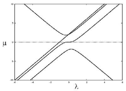
Figure 1: The eigenvalue curve of the pencil of the quadrics $(y^{2}+2\,x\,z+1,\ 2\,y\,z+1)$.

Index sequence: Let $\lambda_{j}$, $j=1,2,\dots,r$, be all distinct real roots of $f(\lambda)=0$ in increasing order. Let $\mu_{k}$, $k=1,2,\dots,r-1$, be any real numbers separating the $\lambda_{j}$, i.e.,

$$-\infty<\lambda_{1}<\mu_{1}<\lambda_{2}<\dots\mu_{r-1}<\lambda_{r}<\infty.$$

Denote $s_{j}=\textrm{Id}(\mu_{j})$, $j=1,2,\dots,r-1$. Denote $s_{0}=\textrm{Id}(-\infty)$ and $s_{r}=\textrm{Id}(\infty)$. Then the index sequence of $\mathcal{A}$ and $\mathcal{B}$ is defined as

$$\langle s_{0}\uparrow s_{1}\uparrow\dots\uparrow s_{r-1}\uparrow s_{r}\rangle,$$

where $\uparrow$ stands for a real root, single or multiple, of $f(\lambda)=0$.

To distinguish different types of multiplicity of a real root, we use $|$ to denote a real root associated with a $1\times 1$ Jordan block, and use $\wr$ for $p$ consecutive times to denote a real root associated with a $p\times p$ Jordan block. For example, a real root with Segre characteristic $[11]$ will be denoted by $||$ in place of an $\uparrow$ in the index sequence, and a real root with the Segre characteristic $[21]$ will be denoted by ${\wr\wr}|$ in place of an $\uparrow$. When the Segre characteristic is $(22)$, we use $\widehat{\wr\wr}\widehat{\wr\wr}$ to distinguish it from ${\wr\wr}{\wr\wr}$, which has the Segre characteristic $[4]$. Supposing that $\lambda_{0}$ is a real zero of $f(\lambda)$ with a Jordan block of size $k\times k$, we use $\wr\cdots\wr_{+}$ or $\wr\cdots\wr_{-}$ to indicate that the corresponding sign $\varepsilon_{i}$ of the block in the Quadric Pair Canonical Form is $+$ or $-$.

Since $\lambda$ is a projective parameter, a projective transformation $\lambda^{\prime}=(a\lambda+b)/(c\lambda+d)$ does not change the pencil but may change the index sequence of the pencil. On the other hand, thinking of the projective real line of $\lambda$ as a circle topologically, such a transformation induces either a rotation or a reversal of order of the index sequence of the pencil. Therefore we need to define an equivalence relation of all index sequences of a quadric pencil under projective transformations of $\lambda$. In addition, replacing $A$ and $B$ by $-A$ and $-B$ changes each index $s_{i}$ to $\textrm{rank}(\lambda A-B)-s_{i}$ but essentially does not change the pencil $\lambda A-B$. Note that the above replacement changes of the sign associated with a Jordan block of a root; for instance, if the quadrics $A$ and $B$ have the index sequence $\langle 2{\wr\wr}_{-}2|3|2\rangle$, then $-A$ and $-B$ have the index sequence $\langle 2{\wr\wr}_{+}2|1|2\rangle$.

We choose a representative in an equivalence class such that $A$ is nonsingular; therefore, $\infty$ is not a root of $f(\lambda)=0$ and $s_{0}+s_{r}=4$. Taking these observations and conventions into consideration and denoting the equivalence relation by $\sim$, this equivalence of index sequences is then defined by the following three rules:

1) Rotation equivalence:

$$\langle s_{0}\uparrow s_{1}\uparrow\dots\uparrow s_{r-1}\uparrow s_{r}\rangle \sim \langle 4-s_{r-1}\uparrow s_{0}\uparrow s_{1}\uparrow\dots\uparrow s_{r-1}\rangle,$$ (2)

$$\langle s_{0}\uparrow s_{1}\uparrow\dots\uparrow s_{r-1}\uparrow s_{r}\rangle \sim \langle s_{1}\uparrow s_{2}\uparrow\dots\uparrow s_{r}\uparrow 4-s_{1}\rangle.$$

2) Reversal equivalence:

$$\langle s_{0}\uparrow s_{1}\uparrow\dots\uparrow s_{r-1}\uparrow s_{r}\rangle\sim\langle s_{r}\uparrow s_{r-1}\uparrow\dots\uparrow s_{1}\uparrow s_{0}\rangle.$$ (3)

3) Complement equivalence:

$$\langle s_{0}\uparrow s_{1}\uparrow\dots\uparrow s_{r-1}\uparrow s_{r}\rangle\sim\langle 4-s_{0}\uparrow 4-s_{1}\uparrow\dots\uparrow 4-s_{r-1}\uparrow 4-s_{r}\rangle.$$ (4)

2.5 Signature variation

In this section we analyze the behavior of the eigenvalues of the pencil $H(\lambda)=\lambda A-B$, near the roots of $f(\lambda)=\det(H(\lambda))=0$. This analysis amounts to analyzing the eigenvalue curves at a real root of $f(\lambda)$, and is needed for computing the jump of the index function at the real root.

Consider a transformation $H^{\prime}(\lambda)=P^{T}H(\lambda)P$ of $H(\lambda)$, where $P$ is an invertible matrix. First, we compare the behavior of the eigenvalues of $H^{\prime}(\lambda)$ and $H(\lambda)$. For any real symmetric matrix $Q$ of size $n$, we denote by $\rho_{k}(Q)$ the $k^{\text{{th}}}$ real eigenvalue of $Q$, so that $\rho_{1}(Q)\leqslant\rho_{2}(Q)\leqslant\cdots\leqslant\rho_{n}(Q)$. Using the Courant-Fischer Maximin Theorem (see (Golub and van Loan, 1989) p. 403), we have the following result:

$$\rho_{k}(Q)\sigma_{1}(P)^{2}\leqslant\rho_{k}(P^{T}QP)\leqslant\rho_{k}(Q)\sigma_{n}(P)^{2},$$ (5)

where $\sigma_{1}(P)$ (resp. $\sigma_{n}(P)$) is the smallest (resp. largest) singular value of $P$.

Proposition 1

Let $P$ be an invertible matrix and $H^{\prime}(\lambda)=P^{T}H(\lambda)P$. If $\rho_{k}(H(\lambda))=a\lambda^{\mu}(1+o(\lambda))$ with $a\neq 0$, then $\rho_{k}(H^{\prime}(\lambda))=a^{\prime}\lambda^{\mu}(1+o(\lambda))$ with ${\mathrm{sign}}(a)={\mathrm{sign}}(a^{\prime})$.

Proof As the eigenvalue $\rho_{k}(H^{\prime}(\lambda))$ has a Puiseux expansion  (Abhyankar, 1990; Walker, 1962) near $\lambda=0$ of the form $\rho_{k}(H^{\prime}(\lambda))=\rho^{\prime}+a^{\prime}\lambda^{\mu^{\prime}}(1+o(\lambda))$ with $\rho^{\prime},a^{\prime}\in\mathbb{R}$ and $\mu^{\prime}\in\mathbb{Q}$, we deduce from the inequalities (5) that $\rho^{\prime}=0$, $\mu^{\prime}=\mu$ and ${\mathrm{sign}}(a^{\prime})={\mathrm{sign}}(a)$.

Proposition 1 allows us to deduce the behavior of the eigenvalues of the pencil $H(\lambda)$, from its normal form. Indeed, by Theorem 1, $H(\lambda)$ is equivalent to

$$D(\lambda)=\textrm{diag}(\varepsilon_{1}E_{1}(\lambda I_{1}-J_{1}(\lambda_{1})),\varepsilon_{2}E_{2}(\lambda I_{2}-J_{2}(\lambda_{2})),\dots,\varepsilon_{r}E_{r}(\lambda I_{r}-J_{r}(\lambda_{r})),D^{\prime}(\lambda)),$$ (6)

where $I_{i}$ is the identity matrix of the same size as that of the Jordan block $J_{i}(\lambda_{i})$ of eigenvalue $\lambda_{i}$, and $\det(D^{\prime}(\lambda))$ has no real roots. Let us denote by $N_{k}(\lambda,\rho,\varepsilon)=\varepsilon E^{k}(\lambda I^{k}-J^{k}(\rho))$ a block of the preceding form, where $k$ is the size of the corresponding matrices. Then we have the following property:

Proposition 2

The eigenvalue branch $\rho(\lambda)$ corresponding to $N_{k}(\lambda,\rho_{0},\varepsilon)$ which vanishes at $\lambda=\rho_{0}$ is of the form

$$\rho=\varepsilon\nu^{k}(1+o(\nu))$$

where $\lambda=\rho_{0}+\nu$.

Proof By an explicit expansion of the determinant $\mathcal{N}(\lambda,u)=\det(N_{k}(\lambda,\rho_{0},\varepsilon)-uI_{k})$ and denoting $\nu=\lambda-\rho_{0}$, we obtain

$$\mathcal{N}(\lambda,u)=\widetilde{\mathcal{N}}(\nu,u)=(-1)^{k}u^{k}+\cdots+(-\varepsilon)^{k-1}(-1)^{\frac{(k-1)(k-2)}{2}+1}u+\varepsilon^{k}(-1)^{\frac{k(k-1)}{2}}\nu^{k}.$$

The vertices of the lower envelop of the Newton polygon of $\widetilde{\mathcal{N}}(\nu,u)$ in the $(u,\nu)$-monomial space are the points $(k,0),(1,0),(0,k)$. By Newton’s theorem (see (Abhyankar, 1990) p. 89), the Puiseux expansion of the root branch which vanishes near $\rho_{0}$ is of the form

$$\rho=\varepsilon\nu^{k}(1+o(\nu)),$$

which completes the proof.

According to Proposition 1, if the pencil $H(\lambda)$ is equivalent to (6), then near each root $\lambda_{i}$, the eigenvalue branches approaching $0$ are of the form $\varepsilon_{i}(\lambda-\lambda_{i})^{k_{i}}(1+o(\lambda-\lambda_{i}))$, where $k_{i}$ is the size of a block of the Quadric Pair Canonical Form (6) of the eigenvalue $\lambda_{i}$ and $\varepsilon_{i}$ is the corresponding sign.

Index Jump: The preceding analysis explains how the index function can change around the real roots of $f(\lambda)=0$. Let $\alpha$ be a real root of $f(\lambda)=0$. Let $\alpha_{-}$ and $\alpha_{+}$ be values sufficiently close to $\alpha$, with $\alpha_{-}<\alpha$ and $\alpha_{+}>\alpha$. Then the index jumps of $\textrm{Id}(\lambda)$ at $\alpha$ are denoted as

$$\begin{array}[]{l}\Delta^{-}(\alpha)=\textrm{Id}(\alpha)-\textrm{Id}(\alpha_{-}),\;\;\Delta^{+}(\alpha)=\textrm{Id}(\alpha_{+})-\textrm{Id}(\alpha),\\ \Delta(\alpha)=\textrm{Id}(\alpha_{+})-\textrm{Id}(\alpha_{-})=\Delta^{-}(\alpha)+\Delta^{+}(\alpha).\end{array}$$

We denote by $\Delta_{i}^{\pm}(\alpha)$ the changes of signature functions of the blocks $N_{k_{i}}(\lambda,\lambda_{i},\varepsilon_{i})$ at $\alpha.$ Clearly, we have

$$\Delta^{\pm}(\alpha)=\sum_{i=1}^{k}\Delta_{i}^{\pm}(\alpha),\;\;\Delta(\alpha)=\sum_{i=1}^{k}\Delta_{i}(\alpha).$$ (7)

Let us describe each $\Delta_{i}^{\pm}(\alpha)$ separately. For any $a\in\mathbb{R}$, we denote $a^{+}=\max(a,0)$ and $a^{-}=\min(a,0)$. Note that $a^{+}+a^{-}=a$.

(1) Jordan block of size $1\times 1$: In this case, clearly, we have the following signature sequence $(\varepsilon_{i}^{-},(0,0),\varepsilon_{i}^{+})$ and the jumps are $\Delta^{-}(\lambda_{i})=\varepsilon_{i}^{-},\Delta^{+}(\lambda_{i})=\varepsilon_{i}^{+}$ and $\Delta(\lambda_{i})=\varepsilon_{i}$.

(2) Jordan block of size $2\times 2$:

$$N_{k_{i}}(\lambda,\lambda_{i},\varepsilon_{i})=\varepsilon_{i}\left[\begin{array}[]{cc}0&\lambda-\lambda_{i}\\ \lambda-\lambda_{i}&-1\end{array}\right].$$

In this case the corresponding eigenvalue branch vanishing at $\lambda_{i}$ is equivalent to $\varepsilon_{i}(\lambda-\lambda_{i})^{2}$; therefore its sign is the same before and after $\lambda_{i}$. There is one positive eigenvalue and one negative eigenvalue before and after $\lambda_{i}$. If $\varepsilon_{i}>0$, we have a positive eigenvalue branch which goes to $0$ at $\lambda_{i}$; otherwise, we have a negative one. Thus, the signature sequence of $N_{k_{i}}(\lambda,\lambda_{i},\varepsilon_{i})$ is $(1,(1-\varepsilon_{i}^{+},1+\varepsilon_{i}^{-}),1)$ and the jumps are $\Delta^{-}(\lambda_{i})=-\varepsilon_{i}^{+},\Delta^{+}(\lambda_{i})=\varepsilon_{i}^{+}$ and $\Delta(\lambda_{i})=0$.

(3) Jordan block of size $3\times 3$: Since

$$N_{k_{i}}(\lambda,\lambda_{i},\varepsilon_{i})=\varepsilon_{i}\left[\begin{array}[]{ccc}0&0&\lambda-\lambda_{i}\\ 0&\lambda-\lambda_{i}&-1\\ \lambda-\lambda_{i}&-1&0\end{array}\right].$$

The corresponding eigenvalue branch is equivalent to $\varepsilon_{i}(\lambda-\lambda_{i})^{3}$, whose sign changes before and after $\lambda_{i}$. If $\varepsilon_{i}>0$, the signature of $N_{k_{i}}(\lambda,\lambda_{i},\varepsilon_{i})$ is $(1,2)$ before $\lambda_{i}$ and $(2,1)$ after. If $\varepsilon_{i}<0$, we exchange the order of the two signatures. Thus, we have the signature sequence $(\varepsilon_{i}^{+}-2\varepsilon_{i}^{-},(1,1),2\varepsilon_{i}^{+}-\varepsilon_{i}^{-})=(1-\varepsilon_{i}^{-},(1,1),1+\varepsilon_{i}^{+})$ and $\Delta^{-}(\lambda_{i})=\varepsilon_{i}^{-},\Delta^{+}(\lambda_{i})=\varepsilon_{i}^{+}$ and $\Delta(\lambda_{i})=\varepsilon_{i}$.

(4) Jordan block of size $4\times 4$: Using a similar argument, we can show that there are two positive eigenvalues and two negative eigenvalues before and after $\lambda_{i}$ and the eigenvalue curve approaching zero has the form $\varepsilon_{i}(\lambda-\lambda_{i})^{4}$. Thus, the signature sequence of $N_{k_{i}}(\lambda,\lambda_{i},\varepsilon_{i})$ is $(2,(2-\varepsilon_{i}^{+},2+\varepsilon_{i}^{-}),2)$ and $\Delta^{-}(\lambda_{i})=-\varepsilon_{i}^{+},\Delta^{+}(\lambda_{i})=\varepsilon_{i}^{+},\Delta(\lambda_{i})=0$.

To summarize, taking into account the sign $\varepsilon_{i}=\pm 1$, we have $\Delta_{i}(\alpha)=\varepsilon_{i}$ if $J_{i}$ has the size $1\times 1$ or $3\times 3$, and $\Delta_{i}(\alpha)=0$ if $J_{i}$ has the size $2\times 2$ or $4\times 4$. The rank of $H(\lambda)$ drops by $1$ at $\lambda=\lambda_{i}$ for each block of the form $N_{k_{i}}(\lambda,\lambda_{i},\varepsilon_{i})$. Thus, the signature of $H(\lambda_{i})$ can be deduced directly from its index $\mathrm{Id}(\lambda_{i})$ and the number of Jordan blocks with eigenvalue $\lambda_{i}$.

The above rules can be used to decide the permissible index jumps of $\textrm{Id}(\lambda)$ at a real root of $f(\lambda)=0$, through Eqn. (7) and the signature of $H(\lambda_{i})$. In particular, in the case of a simple root $\lambda_{i}$ of $f(\lambda)=0$, the sign $\varepsilon_{i}$ in the Quadric Pair Canonical Form can be deduced directly from the index before and after the root. For instance, an index sequence of the form $\langle 1|2|1|2|3\rangle$ corresponds to a sequence of signs $\varepsilon_{1}=+1,\varepsilon_{2}=-1,\varepsilon_{3}=+1,\varepsilon_{4}=+1$, and the signatures at the roots are $(1,2),(1,2),(1,2),(2,1)$, respectively.

Signature sequence: The previous analysis allows us to completely determine the signature sequence of the pencil $H(\lambda)=\lambda A-B$, from its Quadric Pair Canonical Form. For most of the cases, this signature sequence is, as we will see, a characterization of the QSIC. A signature sequence is defined as

$$\langle s_{0},(\cdots(p_{1},n_{1})\cdots),s_{1},\cdots s_{r-1},(\cdots(p_{r},n_{r})\cdots),s_{r}\rangle,$$

where $s_{i}$ is the index of $H(\lambda)$ between two consecutive real roots of $f(\lambda)=0$, $(p_{i},n_{i})$ is the signature of $H(\lambda_{i})$ at a root $\lambda_{i}$ and the number of parentheses is the multiplicity of $\lambda_{i}$. Note that $p_{i}+n_{i}={\rm rank}(\lambda_{i}A-B)$.

The advantage of using the signature sequence over using the index sequence is that we just need to compute the multiplicity of a real root and determine the signature of $\lambda A-B$ at the root; this is a far simpler computation than computing the Jordan block size, which is the information required by the index sequence. Conversion from an index sequence to the corresponding signature sequence is straightforward. For a given pair of quadrics, the signature sequence can be computed easily using only rational arithmetic as described in Section 2.6. Similar equivalence rules to those for index sequences apply to signature sequences as well. The signature sequences of all 35 QSIC morphologies are listed in the third column of Tables 1, 2 and 3.

2.6 Effective issues

Now we discuss how to use rational arithmetic to compute the signature sequence for classifying the QISC morphology of a given pair of quadrics. Consider the polynomial

$$C(\lambda,u)=\det(\lambda A-B-uI)=u^{4}+c_{3}(\lambda)u^{3}+c_{2}(\lambda)u^{2}+c_{1}(\lambda)u+c_{0}(\lambda).$$

The values where the signature changes are defined by $C(\lambda,0)=c_{0}(\lambda)=f(\lambda)=0$. For a fixed $\lambda$, the rank of the corresponding quadratic form is the number of non-zero roots of $C(\lambda,u)=0$. For any fixed $\lambda$, the number of real roots in $u$, counted with multiplicity, is $4$. The signature of $\lambda A-B$ is determined by the rank of $\lambda A-B$ and the number of positive roots of $C(\lambda,u)=0$ in $u$. In the case where the number of real roots equals the degree of the polynomial, the Descartes rule gives an exact counting of the number of positive roots (Basu et al., 2003), and we have the following property:

Theorem 2

For any $\lambda\in\mathbb{R}$,

• the number of positive eigenvalues of $\lambda A-B$ is the number of sign variations of $[1,c_{3}(\lambda),c_{2}(\lambda),c_{1}(\lambda),c_{0}(\lambda)]$.

• the number of negative eigenvalues of $\lambda A-B$ is the number of sign variations of $[1,-c_{3}(\lambda),c_{2}(\lambda),-c_{1}(\lambda),c_{0}(\lambda)]$.

Computing the signature $\lambda A-B$ for $\lambda\in\mathbb{Q}$ is straightforward. Computing its signature at a root of $C(\lambda,0)=f(\lambda)=0$ can also be performed using only rational arithmetic. According to the previous propositions, this reduces to evaluating the sign of $c_{i}(\lambda)$, $i=1\ldots 3$. This problem can be transformed into rational computation as follows. First, we represent a root $\alpha$ of $f(\lambda)=0$ by

• the square-free part $p(\lambda)$ of $f(\lambda)=0$ and

• an isolating interval $[a,b]$ with $a,b\in\mathbb{Q}$ such that $\alpha$ is the only root of $p(\lambda)$ in $[a,b]$.

Isolating intervals can be obtained efficiently in several ways (see, for instance, (Mourrain et al., 2005)). They can even be pre-computed in the case of polynomials of degree 4 (Emiris et al., 2004). In order to compute the sign of a polynomial $g$ at a root $\alpha$ of $f(\lambda)=0$, we use subresultant (or Sturm-Habicht) sequences. We recall briefly the construction here and refer to (Basu et al., 2003) for more details.

Given two polynomials $f(\lambda)$ and $g(\lambda)\in\mathbb{A}[\lambda]$, where $\mathbb{A}$ is the ring of coefficients, we compute the sub-resultant sequence in $\lambda$, defined in terms of the minors of the Sylvester resultant matrix of $f(\lambda)$ and $f^{\prime}(\lambda)g(\lambda)$. This yields a sequence of polynomials $\mathbf{R}(\lambda)=[R_{0}(\lambda),R_{1}(\lambda),\ldots,R_{N}(\lambda)]$ with $R_{i}(\lambda)\in\mathbb{A}[\lambda]$, whose coefficients are in the same ring $\mathbb{A}$.

In our case, we take $\mathbb{A}=\mathbb{Z}$. For any $a\in\mathbb{R}$, we denote by $V_{f,g}(a)$ the number of sign variation of $\mathbf{R}(a)$. Then we have the following property (Basu et al., 2003):

Theorem 3

$$V_{f,g}(a)-V_{f,g}(b) = \#\{\alpha\in[a,b]\ {\rm root\ of}\ f(\lambda)=0\ {\rm where}\ g(\alpha)>0\}-$$

$$\#\{\alpha\in[a,b]\ {\rm root\ of}\ f(\lambda)=0\ {\rm where}\ g(\alpha)<0\}.$$

In particular, if the interval $[a,b]$ is an isolating interval for a root $\alpha$ of $c_{0}(\lambda)=0$, then $V_{f,g}(a)-V_{f,g}(b)$ gives the sign of $g(\alpha)$. Taking $g(\lambda)$ to be the coefficients $c_{i}(\lambda)$ in Theorem 2, this method allows us to exactly compute the signature of $\alpha A-B$, using only rational arithmetic.

Efficient implementations of the algorithms presented here are available in the library synaps and have been applied to classifying QSIC morphologies, based on the signature sequences derived in this paper.

2.7 List of QSIC morphologies

All 35 different morphologies of QSIC are listed in Tables 1 through 3. In the first column are the Segre characteristics with the subscript indicating the number of real roots, not counting multiplicities. The index sequences and signature sequences are given in the second column and the third column, respectively. Here, only one representative is given for each equivalence class associated with the corresponding QSIC morphology; in several cases, there are two equivalence classes associated with one QSIC morphology. The numeral label for each case, from 1 to 35, is given at the left upper corner of each entry in the second column. These labels are referred to in subsequent theorems establishing the relation between the index sequence and the QSIC morphology. Cases 4, 10 and 31 share the same index sequence $\langle 2\rangle$, thus also the same signature sequence $(2)$. Additional simple conditions based on minimal polynomials for distinguishing these three cases are presented in Section 6. Two different index sequences in cases 26 and 34 correspond to the same signature sequences; the discrimination of these two cases is also discussed in Section 6. In the illustration of each QSIC morphology in column four, a solid line or curve stands for a real component and a dashed one depicts an imaginary component. A solid dot indicates a real singular point, which in many cases is a real intersection point of two or more components of a QSIC. An open or closed component is drawn as such in the illustration. Note that, in addition to topological properties, we also take algebraic properties into consideration in defining morphologically different types. For example, a nonsingular QSIC may be vacuous in $\mathbb{PR}^{3}$, so is a QSIC consisting two imaginary conics; these two QSICs are defined to be morphologically different since the former is irreducible algebraically but the latter is not.

3 Classifications of nonsingular QSIC

3.1 $[1111]_{4}$: f$(\lambda)=0$ has four distinct real roots

Theorem 4

Given two quadrics ${\mathcal{A}}$: $X^{T}AX=0$ and ${\mathcal{B}}$: $X^{T}BX=0$, if their characteristic equation $f(\lambda)=0$ has four distinct real roots, then the only possible index sequences are $\langle 1|2|1|2|3\rangle$ and $\langle 0|1|2|3|4\rangle$. Furthermore,

1. (Case 1, Table 1) when the index sequence is $\langle 1|2|1|2|3\rangle$, the QSIC has two closed components;

2. (Case 2, Table 1) when the index sequence is $\langle 0|1|2|3|4\rangle$, the QSIC is vacuous in $\mathbb{PR}^{3}$.

Proof Let $\lambda_{i}$, $i=1,2,3,4$, be the four distinct real roots of $f(\lambda)=0$. By Theorem 1, $A$ and $B$ are simultaneously congruent to

$$\bar{A}={\rm diag}(\varepsilon_{1},\varepsilon_{2},\varepsilon_{3},\varepsilon_{4}),\;\;\;{\rm and}\;\;\;\bar{B}={\rm diag}(\varepsilon_{1}\lambda_{1},\varepsilon_{2}\lambda_{2},\varepsilon_{3}\lambda_{3},\varepsilon_{4}\lambda_{4}),$$

where $\varepsilon_{i}=\pm 1$, $i=1,2,3,4$. Without loss of generality, we suppose that $\lambda_{1}<\lambda_{2}<\lambda_{3}<\lambda_{4}$; this permutation of the diagonal elements can be achieved by a further congruence transformation to $\bar{A}$ and $\bar{B}$.

Clearly, the only possible index sequences are (up to the equivalence rules of Section 2.4) $\langle 1|2|1|2|3\rangle$ and $\langle 0|1|2|3|4\rangle$. Since a pencil with the second index sequence $\langle 0|1|2|3|4\rangle$ contains a positive definite or negative definite quadric, i.e., with the index being 4 or 0, we deduce that the intersection curve is empty in that case.

For the first index sequence $\langle 1|2|1|2|3\rangle$, according to Section 2.5, the sign sequence in the corresponding Quadric Pair Canonical Form is $(\varepsilon_{1}=1,\varepsilon_{2}=-1,\varepsilon_{3}=1,\varepsilon_{4}=1)$. Setting $\bar{A}$ to $A^{\prime}$ and $\bar{B}-\lambda_{4}\bar{A}$ to $B^{\prime}$, we obtain

$$A^{\prime}={\rm diag}(1,-1,1,1),$$

$$B^{\prime}={\rm diag}\left((\lambda_{1}-\lambda_{4}),-(\lambda_{2}-\lambda_{4}),(\lambda_{3}-\lambda_{4}),0\;\right).$$

Consider the affine realization of $\mathbb{PR}^{3}$ by making $y=0$ the plane at infinity. Then ${\mathcal{A}^{\prime}}$ is a sphere, which intersects the $x$-$z$ plane in a unit circle, while the quadric ${\mathcal{B}^{\prime}}$ is an elliptic cylinder with the $w$-axis being its central direction, which intersects the $x$-$z$ plane in an ellipse, since $\lambda_{i}<\lambda_{4}$, $i=1,2,3$. Clearly, if one of the ellipse’s semi-axes is smaller than 1 or both are smaller than 1, the QSIC of ${\mathcal{A}^{\prime}}$ and ${\mathcal{B}^{\prime}}$ has two oval branches (see the left and middle configurations in Figure 2). If both of the ellipse’s semi-axes are greater than 1, ${\mathcal{A}^{\prime}}$ and ${\mathcal{B}^{\prime}}$ have no real intersection points (see the right configuration in Figure 2). We recall the following result from (Finsler, 1937; Uhlig, 1973b): Two quadrics ${\mathcal{A}}:\;X^{T}AX=0$ and ${\mathcal{B}}:\;X^{T}BX=0$ in ${\mathbb{PR}}^{3}$ has no real points if and only if $\lambda_{0}A-B$ is positive definite or negative definite for some real number $\lambda_{0}$. It implies that the index sequence of the pencil cannot be $\langle 1|2|1|2|3\rangle$. This is a contradiction. Hence, the QSIC has two ovals.

Note that none of the semi-axes can be of length $1$, since $f(\lambda)=0$ is assumed to have no multiple roots. We deduce that the QSIC has two closed components when the index sequence is $\langle 1|2|1|2|3\rangle$ and is empty when the index sequence is $\langle 0|1|2|3|4\rangle$. This completes the proof of Theorem 4.

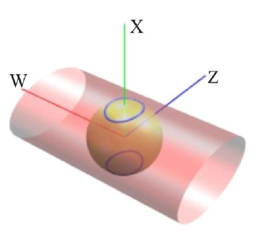
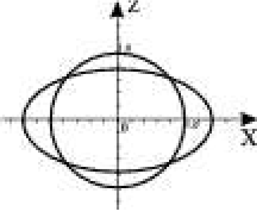
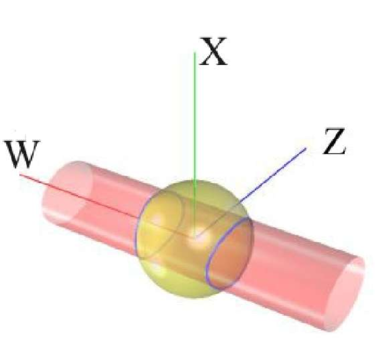
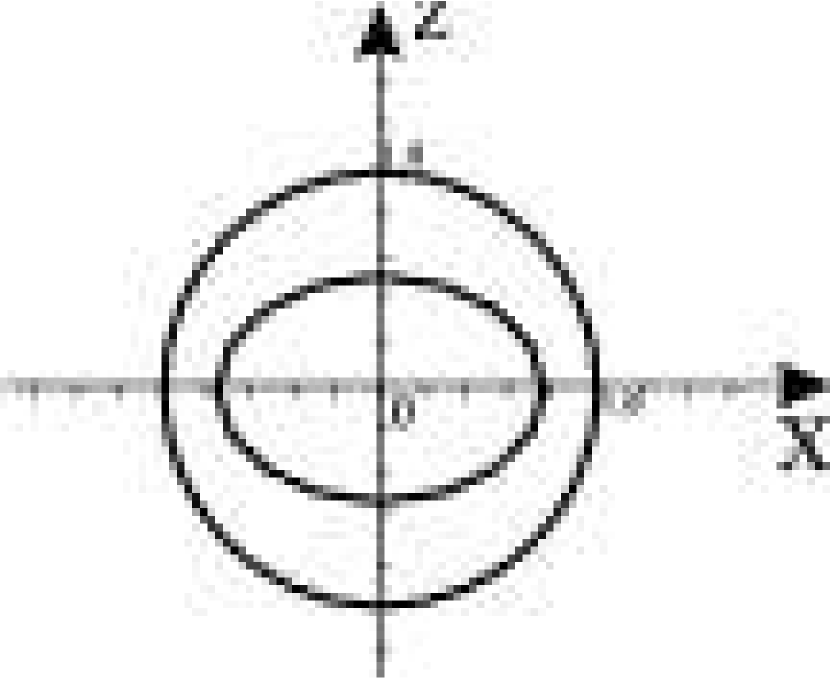
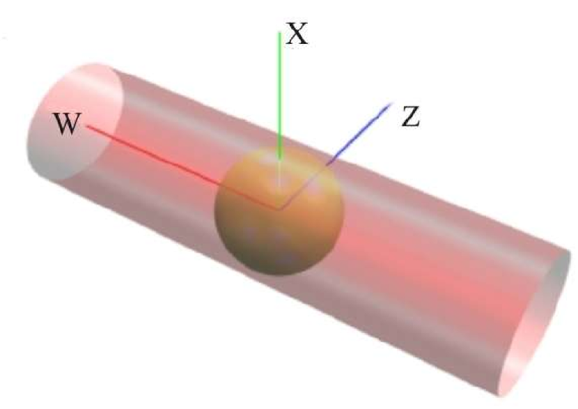
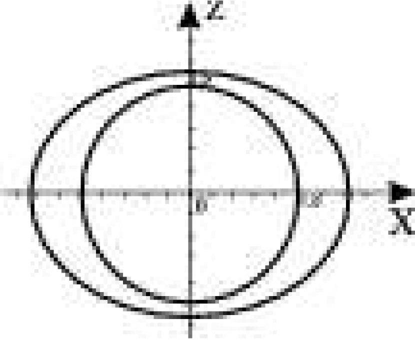
Figure 2: Three cases of an elliptic cylinder intersecting with a unit sphere and their corresponding cross sections in the $x$-$z$ plane.

3.2 $[1111]_{2}$: $f(\lambda)=0$ has two distinct real roots and a pair of complex conjugate roots

Theorem 5

(Case 3, Table 1) If $f(\lambda)=0$ has two distinct real roots and one pair of complex conjugate roots, then the index sequence of the pencil $\lambda A-B$ is $\langle 1|2|3\rangle$, and the QSIC comprises exactly one closed component in $\mathbb{PR}^{3}$.

Proof Wlog, we assume $A$ is nonsingular. Suppose that $f(\lambda)=0$ has two real roots $\lambda_{1}\neq\lambda_{2}$ and two complex conjugate roots $\lambda_{3,4}=a\pm bi$. First, it is easy to see that the only index sequence possible is $\langle 1|2|3\rangle$. We may suppose that $\lambda_{3,4}=\pm i$; this can be done by setting $(B-aA)/b$ to $B$. By Theorem 1, $A$ and $B$ are congruent to

$$A^{\prime}=(a^{\prime}_{ij})={\rm diag}(E_{1},\varepsilon_{1},\varepsilon_{2})={\rm diag}\left(\left(\begin{array}[]{cc}0&1\\ 1&0\end{array}\right),\varepsilon_{1},\varepsilon_{2}\right),$$

$$B^{\prime}=(b^{\prime}_{ij})={\rm diag}(E_{1}J_{1},\varepsilon_{1}\lambda_{1},\varepsilon_{2}\lambda_{2})={\rm diag}(-1,1,\varepsilon_{1}\lambda_{1},\varepsilon_{2}\lambda_{2}).$$

As the index sequence is $\langle 1|2|3\rangle$, we have $\varepsilon_{1}=1,\varepsilon_{2}=1$. Next we need consider two cases: (1) $\lambda_{1}\lambda_{2}\neq 0$ and (2) $\lambda_{1}\lambda_{2}=0$.

Case 1 ($\lambda_{1}\lambda_{2}\neq 0$): By a variable transformation $\lambda^{\prime}=-\lambda$ if necessary, we may assume that at least one of $\lambda_{1}$ and $\lambda_{2}$ is positive. Then we denote $\lambda_{1}>0$ and $\lambda_{2}<0$ if only one of them is positive or denote $\lambda_{2}>\lambda_{1}>0$ if both are positive. It follows that $\frac{\lambda_{1}}{\lambda_{2}}<1$. We then set $\lambda_{1}A^{\prime}-B^{\prime}$ to $A^{\prime}$ and use a further simultaneous congruence transformation to scale the diagonal elements of $B^{\prime}$ into ${\pm 1}$. For simplicity of notation, we use the same symbols $A^{\prime}$ and $B^{\prime}$ for the resulting matrices and obtain

$$A^{\prime}=(a^{\prime}_{ij})=\left(\begin{array}[]{cccc}1&\lambda_{1}&&\\ \lambda_{1}&-1&&\\ &&0&\\ &&&\beta_{2}(\frac{\lambda_{1}}{\lambda_{2}}-1)\end{array}\right),\;B^{\prime}=(b^{\prime}_{ij})=\left(\begin{array}[]{cccc}-1&&&\\ &1&&\\ &&1&\\ &&&\beta_{2}\end{array}\right).$$

where $\beta_{2}=\lambda_{2}/|\lambda_{2}|=\pm 1$.

If $\beta_{2}=1$, we swap $b^{\prime}_{4,4}$ and $b^{\prime}_{1,1}$, as well as $a^{\prime}_{4,4}$ and $a^{\prime}_{1,1}$, to obtain

$$A^{\prime}=\left(\begin{array}[]{cccc}(\frac{\lambda_{1}}{\lambda_{2}}-1)&&&\\ &-1&&\lambda_{1}\\ &&0&\\ &\lambda_{1}&&1\end{array}\right),\;\;\;B^{\prime}=\left(\begin{array}[]{cccc}1&&&\\ &1&&\\ &&1&\\ &&&-1\end{array}\right).$$

Or, if $\beta_{2}=-1$, we swap $b^{\prime}_{4,4}$ and $b^{\prime}_{2,2}$, as well as $a^{\prime}_{4,4}$ and $a^{\prime}_{2,2}$, to obtain

$$A^{\prime}=\left(\begin{array}[]{cccc}1&&&\lambda_{1}\\ &(1-\frac{\lambda_{1}}{\lambda_{2}})&&\\ &&0&\\ \lambda_{1}&&&-1\end{array}\right),\;\;B^{\prime}=\left(\begin{array}[]{cccc}-1&&&\\ &-1&&\\ &&1&\\ &&&1\end{array}\right).$$

Note that permuting diagonal elements can be achieved by a congruence transformation. Hence, whether $\beta_{2}=1$ or $\beta_{2}=-1$, after a proper simultaneous congruence transformation, ${\mathcal{B}^{\prime}}$ is the unit sphere or a one-sheet hyperboloid with the $z$-axis as its central axis. Since $\frac{\lambda_{1}}{\lambda_{2}}<1$, $a^{\prime}_{1,1}$ and $a^{\prime}_{2,2}$ have the same sign. Therefore, ${\mathcal{A}^{\prime}}$ is an elliptic cylinder parallel to the $z$-axis. Due to the symmetry of ${\mathcal{B}^{\prime}}$ and ${\mathcal{A}^{\prime}}$ about the $x$-$y$ plane, we just need to analyze the relationship between the two conic sections in which ${\mathcal{A}^{\prime}}$ and ${\mathcal{B}^{\prime}}$ intersect with the $x$-$y$ plane.

The quadric ${\mathcal{B}^{\prime}}$ intersects the $x$-$y$ plane in the unit circle $x^{2}+y^{2}=w^{2}$, and ${\mathcal{A}^{\prime}}$ intersects the $x$-$y$ plane in the ellipse

$$\frac{x^{2}}{a^{2}}+\frac{(y-cw)^{2}}{b^{2}}=w^{2}$$

when $\beta_{2}=1$, or in the ellipse

$$\frac{(x+cw)^{2}}{b^{2}}+\frac{y^{2}}{a^{2}}=w^{2}$$

when $\beta_{2}=-1$. Here $a=\sqrt{\frac{\lambda_{2}(1+\lambda_{1}^{2})}{(\lambda_{2}-\lambda_{1})}}$, $b=\sqrt{1+\lambda_{1}^{2}}$, and $c=\lambda_{1}$.

In both cases of $\beta_{2}=\pm 1$, the center of the ellipse shifts from the origin (along the $x$ direction or $y$ direction) by the distance $|\lambda_{1}|$, and the length of the ellipse’s semi-axis in the shift direction is $b=\sqrt{1+\lambda_{1}^{2}}$. Then it is straightforward to verify that one of the ellipse’s extreme points of this axis is inside the unit circle, while the other is outside the unit circle. (See Figure 4 for the case of $\beta_{2}=-1$.) In this case the QSIC of ${\mathcal{A}^{\prime}}$ and ${\mathcal{B}^{\prime}}$ has one closed component in $\mathbb{PR}^{3}$ (see Figure 4).

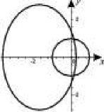
Figure 3: The cross-sections of an elliptic cylinder and a hyperboloid with one sheet in the $x$-$y$ plane.

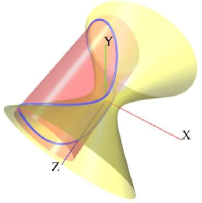
Figure 4: The intersection curve referred to in Figure 4

.

Case 2 ($\lambda_{1}\lambda_{2}=0$): Wlog, we may suppose that $\lambda_{1}=0$ and $\lambda_{2}\neq 0$. Then, by Theorem 1, noting that $\varepsilon_{1}=\varepsilon_{2}=1$, $A$ and $B$ are congruent to

$$A^{\prime}=\left(\begin{array}[]{cccc}0&1&&\\ 1&0&&\\ &&1&\\ &&&1\end{array}\right),\;\;\;B^{\prime}=\left(\begin{array}[]{cccc}-1&0&&\\ 0&1&&\\ &&0&\\ &&&\lambda_{2}\end{array}\right).$$

First set $A^{\prime}-(1/\lambda_{2})B^{\prime}$ to be $A^{\prime}$. Then we use a congruence transformation to make the diagonal elements of $B^{\prime}$ become ${\pm 1}$ and apply the same transformation to $A^{\prime}$. Denoting the resulting matrices again using $A^{\prime}$ and $B^{\prime}$, we obtain

$$A^{\prime}=(a^{\prime}_{ij})=\left(\begin{array}[]{cccc}\frac{1}{\lambda_{2}}&1&&\\ 1&-\frac{1}{\lambda_{2}}&&\\ &&1&\\ &&&0\end{array}\right),\;\;\;\;B^{\prime}=(b^{\prime}_{ij})=\left(\begin{array}[]{cccc}-1&0&&\\ 0&1&&\\ &&0&\\ &&&1\end{array}\right).$$

We swap $b^{\prime}_{4,4}$ and $b^{\prime}_{1,1}$, as well as $a^{\prime}_{4,4}$ and $a^{\prime}_{1,1}$, by a simultaneous congruence transformation to obtain

$$A^{\prime}=\left(\begin{array}[]{cccc}0&&&\\ &-\frac{1}{\lambda_{2}}&&1\\ &&1&\\ &1&&\frac{1}{\lambda_{2}}\end{array}\right),\;\;\;B^{\prime}=\left(\begin{array}[]{cccc}1&&&\\ &1&&\\ &&0&\\ &&&-1\end{array}\right).$$

Thus, ${\mathcal{B}^{\prime}}$ is a cylinder with the $z$-axis as its central axis, and ${\mathcal{A}^{\prime}}$ is either an elliptic cylinder or a hyperbolic cylinder, depending on the sign of $\lambda_{2}$, and ${\mathcal{A}}^{\prime}$ is parallel to the $y$-axis. The equation of ${\mathcal{A}^{\prime}}$ is

$$\frac{(y-cw)^{2}}{a^{2}}\pm\frac{z^{2}}{b^{2}}=w^{2},$$

where $a=\sqrt{1+\lambda_{2}^{2}}$, $b=\sqrt{\frac{1+\lambda_{2}^{2}}{|\lambda_{2}|}}$, $c=\lambda_{2}$. The cylinder ${\mathcal{A}^{\prime}}$ shifts from the origin by the distance $|\lambda_{2}|$ along the $x$-axis or the $y$-axis, and the length of its semi-axis in the shift direction is $\sqrt{1+\lambda_{2}^{2}}$. Clearly, in this case, the QSIC of the cylinders ${\mathcal{A}^{\prime}}$ and ${\mathcal{B}^{\prime}}$ has exactly one closed component in $\mathbb{PR}^{3}$. (See Figure 5.) This completes the proof.

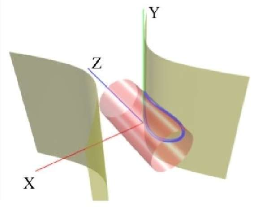
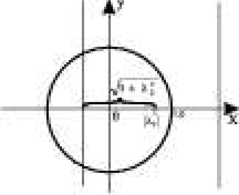
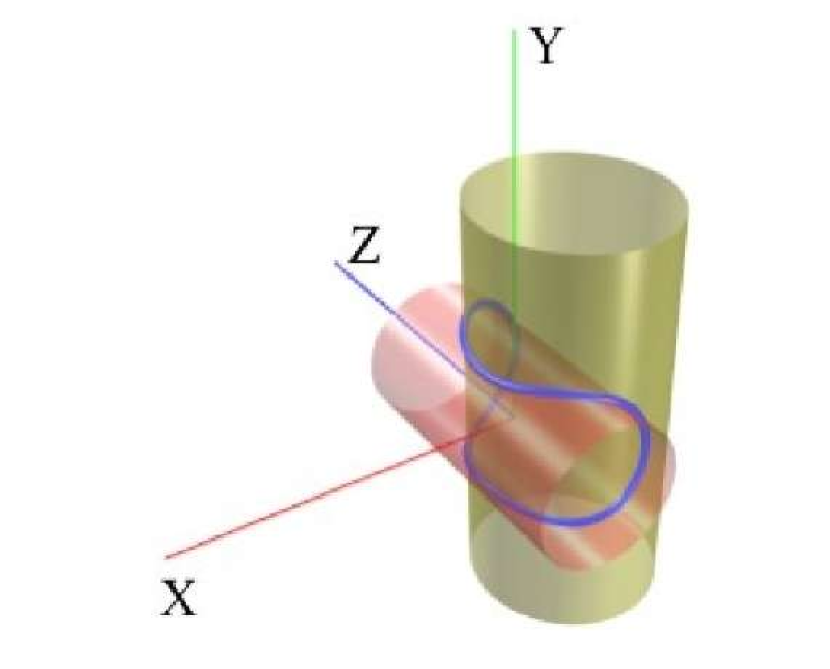
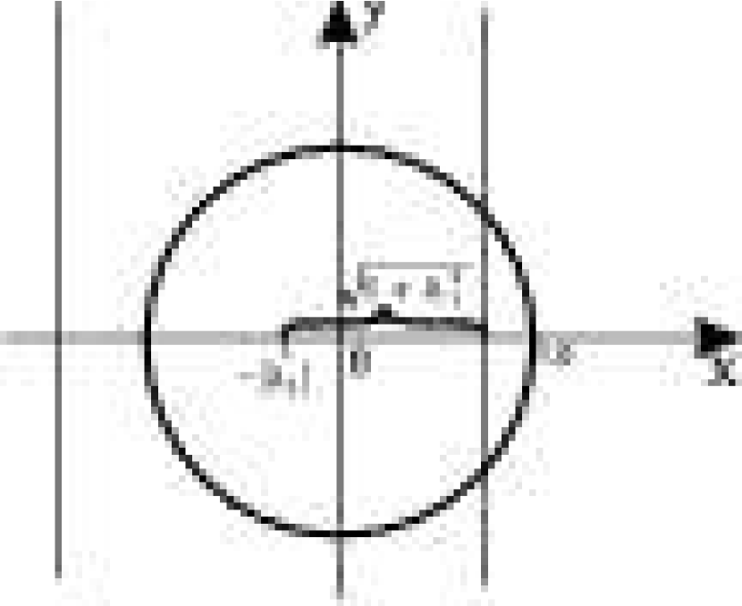
Figure 5: The intersection of a circular cylinder with a hyperbolic cylinder or an elliptic cylinder.

3.3 $[1111]_{0}$: $f(\lambda)=0$ has two distinct pairs of complex conjugate roots

Theorem 6

(Case 4, Table 1) If ${\rm f}(\lambda)=0$ has two distinct pairs of complex conjugate roots, then the Segre characteristic is $[1111]$ and the index sequence is $\langle 2\rangle$. In this case the QSIC comprises two open components in $\mathbb{PR}^{3}$.

Proof Suppose that $f(\lambda)=0$ has the roots $a\pm bi$ and $c\pm di$. First, it is easy to see that the index sequence is $\langle 2\rangle$. By setting $(B-cA)/d$ to be $B$, we transform conjugate roots $c\pm di$ to $\pm i$. Therefore, we suppose that $f(\lambda)=0$ has the roots $a\pm bi$ and $\pm i$. Furthermore, we may suppose that $A$ and $B$ form a nonsingular pair of real symmetric matrices. Then, by Theorem 1, $A$ and $B$ have the following canonical forms

$$A^{\prime}={\rm diag}\left(\left(\begin{array}[]{cc}0&1\\ 1&0\end{array}\right),\left(\begin{array}[]{cc}0&1\\ 1&0\end{array}\right)\right)\;\;{\rm and}\;\;B^{\prime}={\rm diag}\left(\left(\begin{array}[]{cc}-1&\\ &1\end{array}\right),\left(\begin{array}[]{cc}\ -b&a\\ a&b\end{array}\right)\right).$$

Here, $a\neq 0$ or $b\neq\pm 1$, since the roots $a\pm bi$ are distinct from $\pm i$. Also, $b\neq 0$ since $a\pm bi$ are imaginary. Wlog, we may assume $b>0$. In the following we will derive a parameterization of the QSIC from which the topological information about the QSIC can be deduced. The quadric ${\mathcal{A}}^{\prime}:X^{T}A^{\prime}X=0$ is a hyperbolic paraboloid and can therefore be parameterized by ${\bf r}(u,v)={\bf g}(u)+{\bf h}(u)v$ where

$${\bf g}(u)=(-u,0,0,1)^{T}\;\;{\rm and}\;\;{\bf h}(u)=(0,1,u,0)^{T}.$$

Substituting ${\bf r}(u,v)$ into $X^{T}B^{\prime}X=0$ yields

$$v=\frac{-{\bf g}(u)^{T}B^{\prime}{\bf h}(u)\pm\sqrt{s(u)}}{{\bf h}(u)^{T}B^{\prime}{\bf h}(u)},$$ (8)

where

$$\begin{split}s(u)&=[{\bf g}(u)^{T}B^{\prime}{\bf h}(u)]^{2}-[({\bf g}(u)^{T}B^{\prime}{\bf g}(u))({\bf h}(u)^{T}B^{\prime}{\bf h}(u))]\\ &=-bu^{4}+(a^{2}+b^{2}+1)u^{2}-b.\end{split}$$

Substituting (8) into ${\bf r}(u,v)$ yields the following parameterization of the QSIC,

$${\bf p}(u)=\left[bu^{3}-u,-\left(au\pm\sqrt{s(u)}\right),-u\left(au\pm\sqrt{s(u)}\right),1-bu^{2}\right]^{T}.$$ (9)

Since ${\bf p}(u)$ is a real point only when $s(u)\geq 0$, we are going to identify the intervals in which $s(u)\geq 0$ holds. We will first show that $s(u)=0$ always has four distinct real roots. The equation

$$s(u)=-bu^{4}+(a^{2}+b^{2}+1)u^{2}-b=0$$

is a quadratic equation in $u^{2}$ with discriminant

$$\Delta=(a^{2}+b^{2}+1)^{2}-4b^{2}=a^{2}(a^{2}+2b^{2}+2)+(b^{2}-1)^{2}>0,$$

since $a\neq 0$ or $b\neq\pm 1$. Therefore the two real solutions of $u^{2}$ are

$$u^{2}=\frac{(a^{2}+b^{2}+1)\pm\sqrt{\Delta}}{2b}.$$ (10)

Since $\Delta=(a^{2}+b^{2}+1)^{2}-4b^{2}$ and $b\neq 0$, we have $(a^{2}+b^{2}+1)>\sqrt{\Delta}$. It follows that the numerator and denominator in (10) are positive; recall that $b>0$ is assumed. Then we get the four real solutions for $s(u)=0$ from (10), denoted by $\pm u_{+}$ and $\pm u_{-}$, with $u_{+}>u_{-}>0$.

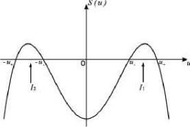
Figure 6: The graph of $s(u)$.

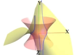
Figure 7: The case of the QSIC has two affinely infinite components.

Define two intervals $I_{1}=[u_{-},u_{+}]$, $I_{2}=[-u_{+},-u_{-}]$. Since $s(0)=-b<0$, we have $s(u)\geq 0$ for $u\in I_{1}\bigcup I_{2}$ and $s(u)<0$ for the other values of $u$. (See Figure 7 for the graph of $s(u)$.) This implies that the QSIC, given by ${\bf p}(u)$, has two connected components, denoted by ${\mathcal{V}}_{1}$ and ${\mathcal{V}}_{2}$, corresponding to the intervals $I_{1}$ and $I_{2}$: ${\mathcal{P}}_{1}$ is defined by ${\bf p}(u)$ over the interval $I_{1}$, and ${\mathcal{V}}_{2}$ is defined by ${\bf p}(u)$ over the interval $I_{2}$.

Next we are going to show that the two components ${\mathcal{V}}_{1}$ and ${\mathcal{V}}_{2}$ are open curves in $\mathbb{PR}^{3}$. Since ${\mathcal{V}}_{1}$ and ${\mathcal{V}}_{2}$ have the same parametric expression ${\bf p}(u)$ but over different intervals, we will only analyze the component ${\mathcal{V}}_{1}$; the analysis for ${\mathcal{V}}_{2}$ is similar. The key idea of the proof is to show that ${\mathcal{V}}_{1}$ has exactly one intersection point with the plane $w=0$; it will then follows that ${\mathcal{V}}_{1}$ has an intersection with every plane in $\mathbb{PR}^{3}$.

Consider the affine realization $\mathbb{AR}^{3}$ of $\mathbb{PR}^{3}$ by making the plane $w=0$ the plane at infinity. The $w$-coordinate component of ${\bf p}(u)$ is $w(u)=1-bu^{2}$, which has two zeros $u_{1}=1/\sqrt{b}$ and $u_{2}=-1/\sqrt{b}$, and it is straightforward to verify that $u_{1}=1/\sqrt{b}\in I_{1}$ and $u_{2}=-1/\sqrt{b}\in I_{2}$. Therefore we will only consider the two points ${\bf p}(u_{1})$ (i.e., with $\pm$ in Eqn. (9)) on the component ${\mathcal{V}}_{1}$. Let ${\bf q}_{0}(u)$ and ${\bf q}_{1}(u)$ denote the two “branches” of ${\bf p}(u)$ corresponding to $\pm$ in front of $\sqrt{s(u)}$ in Eqn. (9). Then

$${\bf q}_{0}(u) = \left(bu^{3}-u,-\left(au+\sqrt{s(u)}\right),-u\left(au+\sqrt{s(u)}\right),1-bu^{2}\right)^{T}$$

$${\bf q}_{1}(u) = \left(bu^{3}-u,-\left(au-\sqrt{s(u)}\right),-u\left(au-\sqrt{s(u)}\right),1-bu^{2}\right)^{T}.$$ (11)

There are now three cases to consider: ($i$) $a=0$; ($ii$) $a>0$; and ($iii$) $a<0$. First consider the case ($i$) $a=0$. In this case,

$$s(u)=-bu^{4}+(b^{2}+1)u^{2}-b=(u^{2}-b)(1-bu^{2}).$$

It follows from Eqn. (11), after dropping a common factor $\sqrt{|1-bu^{2}|}$, that

$${\bf q}_{0}(u) = \left(-u\sqrt{|1-bu^{2}|},-\sqrt{|u^{2}-b|},-u\sqrt{|u^{2}-b|},\sqrt{|1-bu^{2}|}\right)^{T},$$

$${\bf q}_{1}(u) = \left(-u\sqrt{|1-bu^{2}|},\sqrt{|u^{2}-b|},u\sqrt{|u^{2}-b|},\sqrt{|1-bu^{2}|}\right)^{T}.$$

Note that the two ends of $I_{1}$ are $1/\sqrt{b}$ and $\sqrt{b}$ when $a=0$. It is easy to verify that, when $u=\sqrt{b}$, the two branches ${\bf q}_{0}(u)$ and ${\bf q}_{1}(u)$ are joined together at the finite point

$${\bf q}_{0}(\sqrt{b})={\bf q}_{1}(\sqrt{b})=(-\sqrt{b|1-b^{2}|},0,0,\sqrt{|1-b^{2}|})^{T}.$$

Next consider the behavior of ${\bf q}_{0}(u)$ and ${\bf q}_{1}(u)$ when $u\rightarrow u_{1}=1/\sqrt{b}$, which is the other end of $I_{1}$. Since

$${\bf q}_{0}(u_{1})=(0,-\sqrt{|b^{-1}-b|},-\sqrt{|b^{-1}-b|/b},0)^{T}$$

and

$${\bf q}_{1}(u_{1})=(0,\sqrt{|b^{-1}-b|},\sqrt{|b^{-1}-b|/b},0)^{T},$$

${\bf q}_{0}(u_{1})$ and ${\bf q}_{1}(u_{1})$ represent the same point at infinity.

Denote ${\bf q}_{i}(u)=(x_{i},y_{i},z_{i},w_{i})^{T}$, $i=0,1$. To study the asymptotic behavior of the QSIC, let us consider the limit of the affine coordinates of ${\bf q}_{0}(u)$ and ${\bf q}_{1}(u)$, i.e., $(x_{0}/w_{0},y_{0}/w_{0},z_{0}/w_{0})^{T}$ and $(x_{1}/w_{1},y_{1}/w_{1},z_{1}/w_{1})^{T}$, as $u\rightarrow u_{1}=1/\sqrt{b}$. Clearly,

$$\lim_{u\rightarrow u_{1}}\frac{x_{0}(u)}{w_{0}(u)}=\lim_{u\rightarrow u_{1}}\frac{x_{1}(u)}{w_{1}(u)}=-\frac{1}{\sqrt{b}},$$

$$\lim_{u\rightarrow u_{1}}\frac{y_{0}(u)}{w_{0}(u)}=-\lim_{u\rightarrow u_{1}}\frac{y_{1}(u)}{w_{1}(u)}=-\infty,$$

and

$$\lim_{u\rightarrow u_{1}}\frac{z_{0}(u)}{w_{0}(u)}=-\lim_{u\rightarrow u_{1}}\frac{z_{1}(u)}{w_{1}(u)}=-\infty.$$

Therefore, the component curve ${\mathcal{V}}_{1}$ comprises one connected component and its two ends extend to infinity in opposite directions in ${\mathbb{AR}}^{3}$, with its asymptote line being the intersection line of the two planes $x+u_{1}w=0$ and $-u_{1}y+z=0$. Clearly, ${\mathcal{V}}_{1}$ is intersected by every plane in $\mathbb{PR}^{3}$. Hence, ${\mathcal{V}}_{1}$ is open in $\mathbb{PR}^{3}$.

Now we consider case ($ii)$: $a>0$. In this case, $u_{1}=1/\sqrt{b}\in I_{1}=(u_{-},u_{+})$. Clearly, the two parts of ${\mathcal{V}}_{1}$ defined by ${\bf q}_{0}(u)$ and ${\bf q}_{1}(u)$ are joined at the two finite points $q_{0}(u_{-})=q_{1}(u_{-})$ and $q_{0}(u_{+})=q_{1}(u_{+})$ We will show that, when $u=u_{1}=1/\sqrt{b}$, ${\bf q}_{0}(u_{1})$ gives the only infinite point on ${\mathcal{V}}_{1}$. Since, from Eqn. (11),

$${\bf q}_{0}(u_{1})=(0,-2a/\sqrt{b},-2a/b,0)^{T},$$

${\bf q}_{0}(u_{1})$ is a point at infinity. To study how ${\bf q}_{0}(u)$ approach the infinite point ${\bf q}_{0}(u_{1})$, let us consider the $\lim_{u\rightarrow u_{1-}}{\bf q}_{0}(u)$ and $\lim_{u\rightarrow u_{1+}}{\bf q}_{0}(u)$ when $u$ approaches $u_{1}$ from different sides. Using the affine coordinates of ${\bf q}_{0}(u)$, we have

$$\lim_{u\rightarrow u_{1-}}\frac{x_{0}(u)}{w_{0}(u)}=-\lim_{u\rightarrow u_{1+}}\frac{x_{0}(u)}{w_{0}(u)}=-1/\sqrt{b},$$

$$\lim_{u\rightarrow u_{1-}}\frac{y_{0}(u)}{w_{0}(u)}=-\lim_{u\rightarrow u_{1+}}\frac{y_{0}(u)}{w_{0}(u)}=+\infty,$$

and

$$\lim_{u\rightarrow u_{1-}}\frac{z_{0}(u)}{w_{0}(u)}=-\lim_{u\rightarrow u_{1+}}\frac{z_{0}(u)}{w_{0}(u)}=+\infty.$$

Thus, the component ${\mathcal{V}}_{1}$ extends to infinity in opposite directions, with its asymptote being the intersection line of the two planes $x+u_{1}w=0$ and $-u_{1}y+z=0$.

Note that all other points of ${\mathcal{V}}_{1}$ are obviously finite, except for the point ${\bf q}_{1}(u_{1})$ whose $w$ component is zero. But we will show that ${\bf q}_{1}(u_{1})$ is, in fact, also a finite point. Denote $g(u)=\sqrt{s(u)}$. Expanding $g(u)$ at $u=u_{1}$ by the Taylor formula yields

$$g(u)=\frac{a}{\sqrt{b}}+g^{\prime}(u_{1})(u-u_{1})+o(u-u_{1}),$$

where $o(u-u_{1})$ is a term whose order is higher than $u-u_{1}$ when $u\rightarrow u_{1}$. Plugging the above $g(u)$ in ${\bf q}_{1}(u)$ yields

$${\bf q}_{1}(u) = \left(bu^{3}-u,-(au-g(u)),-u(au-g(u)),1-bu^{2}\right)^{T}$$

$$= \left(\begin{array}[]{c}bu(u+1/\sqrt{b})(u-1/\sqrt{b})\\ -\left(au-a/\sqrt{b}-g^{\prime}(u_{1})(u-1/\sqrt{b})\right)\\ -u\left(au-q/\sqrt{b}-g^{\prime}(u_{1})(u-1/\sqrt{b})\right)\\ -b(u+1/\sqrt{b})(u-1/\sqrt{b})\end{array}\right)+o(u-u_{1})$$

$$= \left(\begin{array}[]{c}bu(u+1/\sqrt{b})(u-1/\sqrt{b})\\ (g^{\prime}(u_{1})-a)(u-1/\sqrt{b})\\ u(g^{\prime}(u_{1})-a)(u-1/\sqrt{b})\\ -b(u+1/\sqrt{b})(u-1/\sqrt{b})\end{array}\right)+o(u-u_{1}).$$

Dividing a common factor $u-u_{1}=u-1/\sqrt{b}$ to these homogeneous coordinates, we have

$${\bf q}_{1}(u)=\left(bu(u+1/\sqrt{b}),g^{\prime}(u_{1})-a,u(g^{\prime}(u_{1})-a),-b(u+1/\sqrt{b})\right)^{T}+o(1)$$

Therefore,

$$\lim_{u\rightarrow u_{1}}{\bf q}_{1}(u)=\left(2,\;\;g^{\prime}(u_{1})-a,\;\;(g^{\prime}(u_{1})-a)/\sqrt{b},\;\;-2\sqrt{b}\right)^{T}.$$

It follows that ${\bf q}_{1}(u_{1})$ is a finite point in $\mathbb{AR}^{3}$. Hence, ${\mathcal{V}}_{1}$ is an open curve in $\mathbb{PR}^{3}$, since it is a continuous curve that extends to infinity in opposite directions with an asymptote line.

In the third case of $a<0$, it can be proved similarly that ${\bf q}_{0}(u_{1})$ is a finite point in $\mathbb{AR}^{3}$ and ${\bf q}_{1}(u_{1})$ is the only infinite point on ${\mathcal{V}}_{1}$. Therefore, in this case ${\mathcal{V}}_{1}$ is also an open curve. Finally, in all the three subcases (i.e., $a=0$, $a>0$ and $a<0$), we can show similarly that the other component ${\mathcal{V}}_{2}$ of the QSIC of ${\mathcal{A}}$ and ${\mathcal{B}}$ is also open in $\mathbb{PR}^{3}$. Hence, the QSIC of ${\mathcal{A}}$ and ${\mathcal{B}}$ has two open components in $\mathbb{PR}^{3}$. An example of such a QSIC is shown in Figure 7. This completes the proof of Theorem 6.

4 Classification of singular but non-planar QSIC

4.1 $[211]$: $f(\lambda)=0$ has one real double root and two other distinct roots

Theorem 7

($[211]_{3}$) Given two quadrics ${\mathcal{A}}$:$X^{T}AX=0$ and ${\mathcal{B}}$:$X^{T}BX=0$, if $f(\lambda)=0$ has one double real root and two distinct real roots with the Segre characteristic $[211]$, then the only possible index sequences of the pencil $\lambda A-B$ are $\langle 2{\wr\wr}_{-}2|3|2\rangle$, $\langle 2{\wr\wr}_{+}2|3|2\rangle$, $\langle 1{\wr\wr}_{-}1|2|3\rangle$ and $\langle 1{\wr\wr}_{+}1|2|3\rangle$. Furthermore,

1. (Case 5, Table 1) when the index sequence is $\langle 2{\wr\wr}_{-}2|3|2\rangle$ or $\langle 2{\wr\wr}_{+}2|3|2\rangle$, the QSIC has one closed component with a crunode;

2. (Case 6, Table 1) when the index sequence is $\langle 1{\wr\wr}_{-}1|2|3\rangle$, the QSIC has a closed component plus an acnode;

3. (Case 7, Table 1) when the index sequence is $\langle 1{\wr\wr}_{+}1|2|3\rangle$, the QSIC has only one real point, which is an acnode.

Proof Suppose that $f(\lambda)=0$ has one double real root $\lambda_{0}$ and two distinct real roots $\lambda_{1}$ and $\lambda_{2}$ with the Segre characteristic $[211]$. First, it is easy to check that the only possible index sequences are $\langle 2{\wr\wr}_{-}2|3|2\rangle$, $\langle 2{\wr\wr}_{+}2|3|2\rangle$, $\langle 1{\wr\wr}_{-}1|2|3\rangle$ and $\langle 1{\wr\wr}_{+}1|2|3\rangle$.

By setting $B-\lambda_{0}A$ to be $B$, we can transform the double root $\lambda_{0}$ into $0$. With a further projective transform to $\lambda$, we may assume that $0<\lambda_{1}<\lambda_{2}$. According to Theorem 1, and wlog, assuming $\varepsilon_{0}=1$, the two quadrics can be reduced simultaneously to the following forms:

$$A^{\prime}=(a^{\prime}_{ij})=\left(\begin{array}[]{cccc}0&1&0&0\\ 1&0&0&0\\ 0&0&\varepsilon_{1}&0\\ 0&0&0&\varepsilon_{2}\end{array}\right),\;\;B^{\prime}=(b^{\prime}_{ij})=\left(\begin{array}[]{cccc}0&0&0&0\\ 0&1&0&0\\ 0&0&\varepsilon_{1}\lambda_{1}&0\\ 0&0&0&\varepsilon_{2}\lambda_{2}\end{array}\right),$$

where $\varepsilon_{1,2}=\pm 1$. By swapping the position $a^{\prime}_{1,1}$ and $a^{\prime}_{4,4}$, as well as $b^{\prime}_{1,1}$ and $b^{\prime}_{4,4}$, we obtain

$$A^{\prime}=\left(\begin{array}[]{cccc}\varepsilon_{2}&0&0&0\\ 0&0&0&1\\ 0&0&\varepsilon_{1}&0\\ 0&1&0&0\end{array}\right),\;\;B^{\prime}=\left(\begin{array}[]{cccc}\varepsilon_{2}\lambda_{2}&0&0&0\\ 0&1&0&0\\ 0&0&\varepsilon_{1}\lambda_{1}&0\\ 0&0&0&0\end{array}\right).$$

There are now two cases to consider: ($i$) $\det(A^{\prime})>0$ and ($ii$) $\det(A^{\prime})<0$. In case ($i$) (det$(A^{\prime})>0$), we have $\varepsilon_{1}\varepsilon_{2}=-1$. Because Id($\infty$)= index($A^{\prime}$)= 2 and the index jump of index function at $\lambda_{0}=0$ is 0, the associated index sequence is $\langle 2{\wr\wr}_{-}2|3|2\rangle$ or $\langle 2{\wr\wr}_{+}2|3|2\rangle$. Note that $\langle 2{\wr\wr}_{-}2|3|2\rangle$ is equivalent to $\langle 2{\wr\wr}_{+}2|1|2\rangle$, and $\langle 2{\wr\wr}_{+}2|3|2\rangle$ is equivalent to $\langle 2{\wr\wr}_{-}2|1|2\rangle$.

By setting $\frac{\lambda_{1}+\lambda_{2}}{2}A^{\prime}-B^{\prime}$ to be $A^{\prime}$, we obtain

$$A^{\prime}=\left(\begin{array}[]{cccc}\varepsilon_{2}\frac{\lambda_{1}-\lambda_{2}}{2}&0&0&0\\ 0&-1&0&\varepsilon_{1}\frac{\lambda_{1}+\lambda_{2}}{2}\\ 0&0&\frac{\lambda_{2}-\lambda_{1}}{2}&0\\ 0&\varepsilon_{1}\frac{\lambda_{1}+\lambda_{2}}{2}&0&0\end{array}\right),\;\;B^{\prime}=\left(\begin{array}[]{cccc}\varepsilon_{2}\lambda_{2}&0&0&0\\ 0&1&0&0\\ 0&0&\varepsilon_{1}\lambda_{1}&0\\ 0&0&0&0\end{array}\right)$$ (14)

Clearly, the quadric ${\mathcal{B}^{\prime}}$ is a cone passing through the point $(0,0,0,1)^{T}$. Since $\lambda_{2}-\lambda_{1}>0$, ${\mathcal{A}^{\prime}}$ is an ellipsoid if $\varepsilon_{1}=-1$ and $\varepsilon_{2}=1$, and is a two-sheet hyperboloid if $\varepsilon_{1}=1$ and $\varepsilon_{2}=-1$. In both cases ${\mathcal{A}^{\prime}}$ passes through the point $(0,0,0,1)^{T}$. According to Eqn. (14), ${\mathcal{A}^{\prime}}$ and ${\mathcal{B}^{\prime}}$ are in one of the two cases shown in Figure 9. Thus, the QSIC is a singular quartic having one component with a crunode. Because the QSIC is contained in the ellipsoid or two-sheet hyperboloid ${\mathcal{A}^{\prime}}$, it is a closed curve in $\mathbb{PR}^{3}$. This proves the first item of Theorem 7.

Figure 8: Two cases of the QSIC having a crunode.

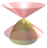
Figure 9: The case of the QSIC having an acnode.

In case ($ii$) (det$(A^{\prime})<0$): $\varepsilon_{1}$ and $\varepsilon_{2}$ have the same sign and Id($\infty$) = Id($A^{\prime}$)= 1 or 3. Also, the index jump at $\lambda_{0}=0$ is $0$ because the size of its Jordan block associated with $\lambda_{0}$ is 2. Therefore, the associated index sequence is $\langle 1{\wr\wr}_{-}1|2|3\rangle$ or $\langle 1{\wr\wr}_{+}1|2|3\rangle$.

If $\varepsilon_{1}=\varepsilon_{2}=-1$, the index of $\lambda_{0}A^{\prime}-B^{\prime}=-B^{\prime}$ is 2. Thus the index sequence is $\langle 3{\wr\wr}_{+}3|2|1\rangle$, which is equivalent to $\langle 1{\wr\wr}_{-}1|2|3\rangle$. In this case the quadric ${\mathcal{B}^{\prime}}$ is a cone with the $y$-axis as its central axis, and the quadric ${\mathcal{A}^{\prime}}$ is an elliptic paraboloid also with $y$-axis as its central axis. It is then easy to verify that the the QSIC has a closed component plus an acnode, as shown in Figure 9. This proves the second item of Theorem 7.

If $\varepsilon_{1}=\varepsilon_{2}=1$, the index of $\lambda_{0}A^{\prime}-B^{\prime}=-B^{\prime}$ is 0. Thus the index sequence $\langle 1{\wr\wr}1|2|3\rangle$ specializes to $\langle 1{\wr\wr}_{+}1|2|3\rangle$. In this case, $B^{\prime}$ is a positive semi-definite; thus, the QSIC of ${\mathcal{A}^{\prime}}:X^{T}A^{\prime}X=0$ and ${\mathcal{B}^{\prime}}:X^{T}B^{\prime}X=0$ has only one real point $(0,0,0,1)$, which can be verified to be an acnode. This proves the last item of Theorem 7.

Theorem 8

($[211]_{1}$: Case 8, Table 1) If $f(\lambda)=0$ has one double root and a pair of complex conjugate roots, then the only possible index sequence is $\langle 2{\wr\wr}_{-}2\rangle$ (or its equivalent $\langle 2{\wr\wr}_{+}2\rangle$) and in this case the QSIC comprises one open component with a crunode.

Proof Suppose that the pair of complex conjugate roots are $a\pm bi$ and the double root is $\lambda_{0}$. Setting $B$ to be $(B-aA)/b$, we transform the roots $a\pm bi$ to $\pm i$. By Theorem 1, the two quadrics can be reduced to the following forms:

$$A^{\prime}=\left(\begin{array}[]{cccc}0&\varepsilon&0&0\\ \varepsilon&0&0&0\\ 0&0&0&1\\ 0&0&1&0\end{array}\right),\;\;B^{\prime}=\left(\begin{array}[]{cccc}0&\varepsilon\lambda_{0}&0&0\\ \varepsilon\lambda_{0}&\varepsilon&0&0\\ 0&0&-1&0\\ 0&0&0&1\end{array}\right),$$ (15)

where $\varepsilon=\pm 1$. Setting $B^{\prime}-\lambda_{0}A$ to be $B^{\prime}$, and then swapping $A^{\prime}_{1,1}$, $A^{\prime}_{4,4}$, as well as $B^{\prime}_{1,1}$, $B^{\prime}_{4,4}$, $A^{\prime}$ and $B^{\prime}$ are transformed to

$$A^{\prime}=\left(\begin{array}[]{cccc}0&0&1&0\\ 0&0&0&\varepsilon\\ 1&0&0&0\\ 0&\varepsilon&0&0\end{array}\right),\;\;B^{\prime}=\left(\begin{array}[]{cccc}1&0&-\lambda_{0}&0\\ 0&\varepsilon&0&0\\ -\lambda_{0}&0&-1&0\\ 0&0&0&0\end{array}\right).$$

Denote $k=1/\sqrt{1+\lambda_{0}^{2}}$. Applying the congruence transformation $C=P^{T}DP$ with

$$P=\left(\begin{array}[]{cccc}1&0&k\lambda_{0}&0\\ 0&1&0&0\\ 0&0&k&0\\ 0&0&0&1\end{array}\right).$$

simultaneously to ${\mathcal{A}^{\prime}}$ and ${\mathcal{B}^{\prime}}$, we obtain the transformed $A^{\prime}$ and $B^{\prime}$ as

$$A^{\prime}=\left(\begin{array}[]{cccc}0&0&k&0\\ 0&0&0&\varepsilon\\ k&0&2k^{2}\lambda_{0}&0\\ 0&\varepsilon&0&0\end{array}\right),\;\;B^{\prime}=\left(\begin{array}[]{cccc}1&0&0&0\\ 0&\varepsilon&0&0\\ 0&0&-1&0\\ 0&0&0&0\end{array}\right).$$

The quadric ${\mathcal{B}}^{\prime}$ is a cone and therefore can be parameterized by

$${\bf r}(u,v)={\bf g}(u)+v{\bf h}(u),$$

where ${\bf g}(u)=(1-\varepsilon u^{2},\;2u,\;1+\varepsilon u^{2},\;0)^{T}$ and ${\bf h}(u)=(0,0,0,1)^{T}$. Substituting ${\bf r}(u,v)$ into $X^{T}A^{\prime}X=0$, we obtain a quadratic equation whose two solutions are $v=\infty$, which is trivial, and $v=-{\bf c_{0}}(u)/(2{\bf c_{1}}(u))$. Substituting the latter solution of $v$ into ${\bf r}(u,v)$ yields the parameterization of the QSIC,

$${\bf p}(u)=\left(2\varepsilon u(1-\varepsilon u^{2}),\;4u^{2},\;2\varepsilon u(1+\varepsilon u^{2}),\;k(1-u^{4})+k^{2}\lambda_{0}(1+\varepsilon u^{2})^{2}\;\right)^{T}$$ (16)

From ${\bf p}(u)$, we see that the QSIC passes through the point ${\bf p}_{0}=(0,0,0,1)^{T}$ twice, with $u=0$ or $u=\infty$. Hence, ${\bf p}_{0}$ is a singular point of the QSIC. Furthermore, it is easy to verify that ${\bf p}_{0}$ is a crunode.

In the following we will show that the QSIC has two open branches intersecting at the crunode. Consider the intersection of the QSIC with the plane $w=0$. The last component $w(u)$ of ${\bf p}(u)$ in Eqn. (16) is a quadratic polynomial in $u^{2}$, whose two zeros are

$$u^{2}=(-\varepsilon k\lambda_{0}+1)/(k\lambda_{0}-1)$$

and

$$u^{2}=(-\varepsilon k\lambda_{0}-1)/(k\lambda_{0}-1).$$

Recall that $k=1/\sqrt{1+\lambda_{0}^{2}}$, it is straightforward to verify that $w(u)$ has two real zeros in $u$. These two real zeros are $u_{1,2}=\pm(\lambda_{0}+\sqrt{1+\lambda_{0}^{2}})$ when $\varepsilon=1$ or $u_{1,2}=\pm 1$ when $\varepsilon=-1$. We observe that $u_{1}$ and $u_{2}$ have opposite signs and ${\bf p}(u_{1})$ and ${\bf p}(u_{2})$ are two distinct points.

Now we are going to show by contradiction that the QSIC cannot be closed. Assume that the QSIC is closed, i.e., there is an affine realization of ${\mathbb{PR}}^{3}$ in which the QSIC is compact. Note that the plane $w=0$ is not necessarily the plane at infinity in this affine realization. Then the QSIC has a topology shown in Figure 11, having two closed loops joining at the crunode, i.e., like the figure of “8”. Since the crunode corresponds to two parameter values $0$ and $\infty$ of $u$ under the parameterization ${\bf p}(u)$ in Eqn. (16), the two loops must be parameterized over the positive interval $u\in(0,+\infty)$ and the negative interval $u\in(-\infty,0)$, respectively. Now consider again the intersection of the QSIC with the plane $w=0$. If the plane $w=0$ intersects any loop of the QSIC, say the loop defined over the positive interval, there must be at least two intersection points, which should be given by two positive values of $u$ through ${\bf p}(u)$. However, from the preceding discussions we know that there are only two intersections between the QSIC: ${\bf p}(u)$ and the plane $w=0$, which correspond to one positive value and one negative value of $u$. This is a contradiction. Hence, there is no finite loop of the QSIC in any affine realization of the projective space. That is, the QSIC has one open component with a crunode. (An example of such a QSIC is shown in Figure 11.) This completes the proof of Theorem 8.

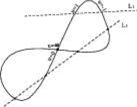
Figure 10: The hypothetical topological shape of a QSIC.

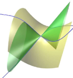
Figure 11: A QSIC having one open component with a crunode.

4.2 $[22]$: f$(\lambda)=0$ has two double roots

Theorem 9

($[22]_{2}$: Case 9, Table 1) If $f(\lambda)=0$ has two real double roots with the Segre characteristic $[22]$, then the only possible index sequences are $\langle 2{\wr\wr}_{-}2{\wr\wr}_{-}2\rangle$ and $\langle 2{\wr\wr}_{-}2{\wr\wr}_{+}2\rangle$, the QSIC comprises a real line and a space cubic curve intersecting at two distinct real points for both sequences.

Theorem 10

($[22]_{0}$: Case 10, Table 1) If $f(\lambda)=0$ has two pairs of identical complex conjugate roots with the Segre characteristic $[22]$, then the index sequences are $\langle 2\rangle$ and the QSIC comprises a real line and a space cubic curve that do not intersect at any real point.

4.3 $[31]$: $f(\lambda)=0$ has one real triple root and one real simple root

Theorem 11

(Case 11, Table 1) If ${\rm f}(\lambda)=0$ has one triple root and one simple real root with the Segre characteristic $[31]$, then the index sequence is $\langle 1{\wr\wr}{\wr}_{+}2|3\rangle$ and the QSIC comprises a closed component with a real cusp.

4.4 $[4]$: $f(\lambda)=0$ has one real quadruple root

Theorem 12

(Case 12, Table 1) If $f(\lambda)=0$ has one quadruple root with the Segre characteristic $[4]$, then the index sequence is $\langle 2{\wr\wr}{\wr\wr}_{-}2\rangle$ or its equivalent form $\langle 2{\wr\wr}{\wr\wr}_{+}2\rangle$, and the QSIC comprises a real line and a real space cubic curve tangent to each other at a real point in this case.

5 Classification of planar QSIC

5.1 $[(11)11]$: $f(\lambda)=0$ has one real double root and two other distinct roots

Theorem 13

($[(11)11]_{3}$) If f$(\lambda)=0$ has one double real root and two distinct real roots with the Segre characteristic $[(11)11]$, then there are only five different possible index sequences and these index sequences correspond to four different QSIC morphologies as follows:

1. (Case 13, Table 2) $\langle 2||2|1|2\rangle$ - two real closed conics intersecting at two distinct real points;

2. (Case 14, Table 2) $\langle 1||3|2|3\rangle$ - two real conics not intersecting at any real points;

3. (Case 15, Table 2) $\langle 1||1|2|3\rangle$ - two imaginary conics intersecting at two distinct real points;

4. (Case 16, Table 2) $\langle 0||2|3|4\rangle$ or $\langle 1||3|4|3\rangle$ - two imaginary conics not intersecting at any real points.

Theorem 14

($[(11)11]_{1}$) If $f(\lambda)=0$ has a real double root $\lambda_{0}$ and a pair of complex conjugate roots with the Segre characteristic $[(11)11]$, then the possible index sequences of the pencil $\lambda A-B$ are $\langle 1||3\rangle$ and $\langle 2||2\rangle$. Furthermore,

1. (Case 17, Table 2) when the index sequence is $\langle 1||3\rangle$, the QSIC comprises of two conics, one real and one imaginary;

2. (Case 18, Table 2) when the index sequence is $\langle 2||2\rangle$, the QSIC comprises of two real conics which cannot both be ellipses simultaneously in any affine realization of ${\mathbb{PR}}^{3}$.

5.2 $[(111)1]_{2}$: $f(\lambda)=0$ has one real triple root and a real simple root

Theorem 15

($[(111)1]_{2}$) If ${\rm f}(\lambda)=0$ has one triple root and a simple root with the Segre characteristic $[(111)1]$, then the only possible index sequences are $\langle 1|||2|3\rangle$ and $\langle 0|||3|4\rangle$. Furthermore,

1. (Case 19, Table 2) when the index sequence is $\langle 1|||2|3\rangle$, the QSIC is a real conic counted twice;

2. (Case 20, Table 2) when the index sequence is $\langle 0|||3|4\rangle$, the QSIC is an imaginary conic counted twice.

5.3 $[(21)1]_{2}$: $f(\lambda)=0$ has one real triple root and a real simple root

Theorem 16

($[(21)1]_{2}$) If ${\rm f}(\lambda)=0$ has one triple root and a simple root with the Segre characteristic $[(21)1]$, then the only possible index sequences are $\langle 1{\wr\wr}_{-}|2|3\rangle$ and $\langle 1{\wr\wr}_{+}|2|3\rangle$. Furthermore,

1. (Case 21, Table 2) when the index sequence is $\langle 1{\wr\wr}_{-}|2|3\rangle$, the QSIC comprises two real conics tangent to each other at one real point;

2. (Case 22, Table 2) when the index sequence is $\langle 1{\wr\wr}_{+}|2|3\rangle$, the QSIC comprises two imaginary conics tangent to each other at one real point.

5.4 $[2(11)]_{2}$: $f(\lambda)=0$ has two real double roots

Theorem 17

If $f(\lambda)=0$ has two double roots with the Segre characteristic $[2(11)]$, then the only possible index sequences are $\langle 2{\wr\wr}_{-}2||2\rangle$ (or its equivalent form $\langle 2{\wr\wr}_{+}2||2\rangle$), $\langle 1{\wr\wr}_{+}1||3\rangle$ and $\langle 1{\wr\wr}_{-}1||3\rangle$. Furthermore,

1. (Case 23, Table 3) when the index sequence is $\langle 2{\wr\wr}_{-}2||2\rangle$, the QSIC consists of a real conic and two real lines which intersect pairwise at three distinct real points;

2. (Case 24, Table 3) when the index sequence is $\langle 1{\wr\wr}_{-}1||3\rangle$, the QSIC consists of a real conic and a pair of complex conjugate lines. The conic and the pair of lines do not intersect;

3. (Case 25, Table 3) when the index sequence is $\langle 1{\wr\wr}_{+}1||3\rangle$, the QSIC consists of an imaginary conic and a pair of complex conjugate lines. The conic and the pair of lines do not intersect.

5.5 $[(31)]_{1}$: $f(\lambda)=0$ has one real quadruple root

Theorem 18

If $f(\lambda)=0$ has one quadruple root with the Segre characteristic $[(31)]$, then the only possible index sequences are $\langle 2{\wr\wr}{\wr}_{-}|2\rangle$ and $\langle 1{\wr\wr}{\wr}_{+}|3\rangle$. Furthermore,

1. (Case 26, Table 3) when the index sequence is $\langle 2{\wr\wr}{\wr}_{-}|2\rangle$, the QSIC consists of a real conic and two real lines, and these three components intersect at a common real point;

2. (Case 27, Table 3) when the index sequence is $\langle 1{\wr\wr}{\wr}_{+}|3\rangle$, the QSIC consists of a real conic and a pair of complex conjugate lines, and these three components intersect at a common real point.

5.6 $[(11)(11)]$: $f(\lambda)=0$ has two double roots

Theorem 19

($[(11)(11)]_{2}$) If $f(\lambda)=0$ has two real double roots with the Segre characteristic $[(11)(11)]$, then the only possible index sequences are $\langle 2||2||2\rangle$, $\langle 0||2||4\rangle$ and $\langle 1||1||3\rangle$. Furthermore,

1. (Case 28, Table 3) when the index sequence is $\langle 2||2||2\rangle$, the QSIC consists of four real lines, and these four lines form a quadrangle in $\mathbb{PR}^{3}$;

2. (Case 29, Table 3) when the index sequence is $\langle 0||2||4\rangle$, the QSIC consists of four imaginary lines and has no real point;

3. (Case 30, Table 3) when the index sequence is $\langle 1||1||3\rangle$, the QSIC consists of two pair of complex conjugate lines, with each pair intersecting at a real point.

Theorem 20

($[(11)(11)]_{0}$: Case 31, Table 3) If $f(\lambda)=0$ has two identical pairs of complex conjugate roots with the Segre characteristic $[(11)(11)]$, the only possible index sequences are $\langle 2\rangle$, and in this case the QSIC comprises two non-intersecting real lines and two non-intersecting imaginary lines.

5.7 $[(211)]$: $f(\lambda)=0$ has one real quadruple root

Theorem 21

If $f(\lambda)=0$ has a quadruple root with the Segre characteristic $[(211)]$, then the only possible index sequences are $\langle 2{\wr\wr}_{-}||2\rangle$ and $\langle 1{\wr\wr}_{-}||3\rangle$. Furthermore,

1. (Case 32, Table 3) when the index sequence is $\langle 2{\wr\wr}_{-}||2\rangle$, the QSIC consists of a pair of intersecting real lines, counted twice;

2. (Case 33, Table 3) when the index sequence is $\langle 1{\wr\wr}_{-}||3\rangle$, the QSIC consists of a pair of conjugate lines, counted twice.

5.8 $[(22)]$: $f(\lambda)=0$ has one real quadruple root

Theorem 22

If $f(\lambda)=0$ has a quadruple root with the Segre characteristic $[(22)]$, then the only possible index sequences are $\langle 2{\wr\wr}_{-}{\wr\wr}_{-}2\rangle$ and $\langle 2{\wr\wr}_{-}{\wr\wr}_{+}2\rangle$ Furthermore,

1. (Case 34, Table 3) when the index sequence is $\langle 2{\wr\wr}_{-}{\wr\wr}_{-}2\rangle$, the QSIC consists a real double line and two other non-intersecting imaginary lines. The two imaginary lines do not form a complex conjugate pair.

2. (Case 35, Table 3) when the index sequence is $\langle 2{\wr\wr}_{-}{\wr\wr}_{+}2\rangle$, the QSIC consists a real double line and two other non-intersecting real lines. Each of the latter two lines intersects the real double line.

6 Classification by signature sequences

Through the above analysis, we have put different QSIC morphologies in correspondence to different characterizing conditions, given by conditions in Theorem 4 through Theorem 22. Hence, we conclude that all these conditions are necessary and sufficient for the corresponding QSIC morphologies. We may then check these conditions to classify the QSIC of a given pair of quadrics in $\mathbb{PR}^{3}$. Based on these conditions one could compute the index sequence of two given quadrics for QSIC classification; however, this would involve the difficult task of computing Jordan blocks. To avoid computing Jordan blocks, we convert all index sequences to their corresponding signature sequences. The advantage of using the signature sequence over using the index sequence is that we just need to compute the multiplicity of a real root and determine the signature of $\lambda A-B$ at the root; this is a far simpler than computing Jordan blocks.

There are some cases which cannot be distinguished by using signature sequences alone. We will show in this section that these cases can easily be distinguished by the fact that their corresponding minimal polynomials have different degrees.

Not all the signature sequences of the 35 different QSIC morphologies are distinct: the three different QSIC morphologies with the Segre characteristics $[1111]_{0}$, $[22]_{0}$ and $[(11)(11)]_{0}$ (i.e., cases 4, 10 and 31) share the same index sequence $\langle 2\rangle$, thus leading to the same signature sequence $(2)$. Furthermore, two different index sequences $\langle 2{\wr\wr}{\wr}_{-}|2\rangle$ and $\langle 2{\wr\wr}_{-}{\wr\wr}_{+}2\rangle$ (i.e., cases 26 and 35) are mapped to the same signature sequence $\langle 2((((1,1))))2\rangle$. Thus, in total, there are only 32 distinct signature sequences. In the following we explain how these cases can be distinguished.

The signature sequence $(2)$ can be given by the different Segre characteristics $[1111]_{0}$, $[22]_{0}$ and $[(11)(11)]_{0}$. Suppose that the signature sequence $(2)$ has been detected, i.e., $f(\lambda)=0$ has been found to have no real root. The case of $[1111]_{0}$ is distinguished from the other two cases by the fact that ${f}(\lambda)=0$ has no multiple roots; this can be detected by whether the discriminant of ${f}(\lambda)$ vanishes, i.e., whether ${\textrm{Disc}}(f)\equiv{\textrm{Res}}_{\lambda}(f,f_{\lambda})=0$.

Then the case of $[22]_{0}$ and the case of $[(11)(11)]_{0}$ can be distinguished by the fact that they have different minimal polynomials. Suppose that the input quadrics are given in the real symmetric matrices $A$ and $B$; and, wlog, assume that $A$ is nonsingular. Since in the case of $[22]_{0}$ or $[(11)(11)]_{0}$, $f(\lambda)$ is a squared polynomial, we suppose

$$f(\lambda)=(a\lambda^{2}+b\lambda+c)^{2},$$

whose square-free part is

$$g(\lambda)=a\lambda^{2}+b\lambda+c,$$

where $a,b,c\in\mathbb{R}$ and $b^{2}-4ac<0$. Then, by Theorem 1 and the Cauchy-Cayley Theorem, the case of $[(11)(11)]_{0}$ occurs if $g(\lambda)$ annihilates $A^{-1}B$, i.e., $g(A^{-1}B)=0$; otherwise, the case of $[22]_{0}$ occurs. Note that $g(\lambda)$ can be obtained as the GCD of $f(\lambda)$ and $f^{\prime}(\lambda)$.

The remaining problem is that the two index sequences $\langle 2{\wr\wr}{\wr}_{-}|2\rangle$ and $\langle 2{\wr\wr}_{-}{\wr\wr}_{+}2\rangle$ are mapped to the same signature sequence $\langle 2((((1,1))))2\rangle$. For either of the two cases, $f(\lambda)=(\lambda-a)^{4}$ for some $a\in\mathbb{R}$, but the minimal polynomial for the case of $\langle 2{\wr\wr}_{-}{\wr\wr}_{+}2\rangle$ is $g(\lambda)=(\lambda-a)^{2}$, while the minimal polynomial for the case of $\langle 2{{\wr\wr}\wr}_{-}|2\rangle$ is $h(\lambda)=(\lambda-a)^{3}$. Therefore, the case of $\langle 2{\wr\wr}_{-}{\wr\wr}_{+}2\rangle$ occurs if $A^{-1}B$ is annihilated by $g(\lambda)$, i.e., $g(A^{-1}B)=0$; otherwise, the case of $\langle 2{\wr\wr}{\wr}_{-}|2\rangle$ occurs. Note that $g(\lambda)=(\lambda-a)^{2}$ can be obtained without solving for the root $a$.

Combining the preceding methods based on minimal polynomials with the methods described in Section 2.6 for exact computation of the signature sequences, we have a complete algorithm for exact classification of QSIC morphologies.

Example 1: Now we use a running example to show the procedure of using the signature sequence for QSIC morphology classification. Consider two quadrics

$$\mathcal{A}:\;\;20\,{x}^{2} - 12\,xy+48\,xz+76\,x+16\,{y}^{2}$$

$$-16\,yz-12\,y+42\,{z}^{2}+72\,z+58=0,$$

$$\mathcal{B}:\;\;28\,{x}^{2} + 16\,xy+80\,xz+56\,x+2\,{y}^{2}$$

$$+24\,yz+20\,y+56\,{z}^{2}+72\,z+14=0.$$

The equation of the eigenvalue curve $\mathcal{C}$ is

$${u}^{4} + \left(-136\,\lambda+100\right){u}^{3}+\left(-1048-3612\,\lambda+2904\,{\lambda}^{2}\right){u}^{2}$$

$$+ \left(-10000\,{\lambda}^{3}+22616\,{\lambda}^{2}+28416\,\lambda\right)u$$

$$- 170528\,{\lambda}^{2}+170528\,{\lambda}^{3}-85264\,{\lambda}^{4}=0.$$

Substituting $u=0$ in this polynomial yields

$$-85264\,{\lambda}^{4}+170528\,{\lambda}^{3}-170528\,{\lambda}^{2}=0,$$

whose only real root is the double root $\lambda=0$. Substituting $\lambda=-1$ in the equation of $\mathcal{C}$ yields

$${u}^{4}+236\,{u}^{3}+5468\,{u}^{2}+4200\,u-426320,$$

which has one sign change in its coefficients; therefore, by the Descartes rule, it has only one positive root. It follows that the signature sequence is $(1,((1,1)),3)$. By Theorem 14, the corresponding QSIC is the union of a real conic and an imaginary one, which is case 17 in Table 2.

7 Conclusions

To summarize, we have obtained the following result:

Theorem 23

There are in total 35 different QSIC morphologies with non-degenerate pencils (see Tables 1, 2 and 3). The morphology of the QSIC of a pencil $(A,B)$ is entirely classified by its signature sequence and the degree of its minimal polynomial, using only rational arithmetic computation.

Besides used for determining the QSIC morphology for enhancing robust computation of QSIC in surface boundary evaluation, another application of our results is to derive simple algebraic conditions for interference analysis of quadrics. For arrangement computation, it is an interesting problem to classify all possible partitions of $\mathbb{R}^{3}$ that can be formed by two ellipsoids. It is also possible to apply the results here to derive efficient algebraic conditions for collision detection between various types of quadric surfaces, such as cones and cylinders, following the framework in (Wang and Krasauskas, 2004).

One could also use the idea developed here to study the classification of a pencil of conics in $\mathbb{PR}^{2}$, which would lead to a classification of QSIC with degenerate pencils in $\mathbb{PR}^{3}$. A more challenging problem is to use the signature sequence to classify the intersection of two quadrics in higher dimensions, $\mathbb{PR}^{4}$ say. Here the difficult issue is to deduce the geometry of the QSIC associated with each possible Quadric Quadric Pair Canonical Form, while it is should be straightforward to obtain the signature sequence of the normal form, based on the results presented in the present paper.

Another direction of investigation would be the classification of the net of three quadrics in $\mathbb{PR}^{n}$. In this case, given three quadratic forms $A$, $B$ and $C$, the question is how to use the invariants of the planar curve $f(\alpha,\beta,\gamma)\equiv\det(\alpha A+\beta B+\gamma C)=0$ to characterize the geometric properties of the net $X^{T}(\alpha A+\beta B+\gamma C)X=0$ or the intersection of the quadrics $X^{T}AX=0$, $X^{T}BX=0$ and $X^{T}CX=0$.

Appendix: Proofs of Theorems 9 Through 22

Proof of Theorem 9 Suppose that the two real double roots are $\lambda_{0}$ and $\lambda_{1}$. By setting $(B-\lambda_{1}A)$ to be $B$, we transform the root $\lambda_{1}$ to 0; the other root is still denoted by $\lambda_{0}$. By Theorem 1, the two quadrics have the canonical forms

$$A^{\prime}=(a^{\prime}_{ij})=\left(\begin{array}[]{cccc}0&1&0&0\\ 1&0&0&0\\ 0&0&0&\varepsilon\\ 0&0&\varepsilon&0\end{array}\right),\;\;B^{\prime}=(b^{\prime}_{ij})=\left(\begin{array}[]{cccc}0&0&0&0\\ 0&1&0&0\\ 0&0&0&\varepsilon\lambda_{0}\\ 0&0&\varepsilon\lambda_{0}&\varepsilon\end{array}\right),$$

where $\varepsilon=\pm 1$. Clearly, Id($A^{\prime}$) = Id($\infty$) = 2 and the index jumps at both roots $\lambda_{0}$ and $\lambda_{1}$ are 0. Therefore the only possible index sequence takes the form $\langle 2{\wr\wr}2{\wr\wr}2\rangle$, covering the two nonequivalent index sequences $\langle 2{\wr\wr}_{-}2{\wr\wr}_{-}2\rangle$ and $\langle 2{\wr\wr}_{-}2{\wr\wr}_{+}2\rangle$. Note that $\langle 2{\wr\wr}_{-}2{\wr\wr}_{-}2\rangle$ is equivalent to $\langle 2{\wr\wr}_{+}2{\wr\wr}_{+}2\rangle$, and $\langle 2{\wr\wr}_{-}2{\wr\wr}_{+}2\rangle$ is equivalent to $\langle 2{\wr\wr}_{+}2{\wr\wr}_{-}2\rangle$.

Swapping $a^{\prime}_{4,4}$ and $a^{\prime}_{1,1}$, as well as $b^{\prime}_{4,4}$ and $b^{\prime}_{1,1}$, we obtain

$$A^{\prime}=\left(\begin{array}[]{cccc}0&0&\varepsilon&0\\ 0&0&0&1\\ \varepsilon&0&0&0\\ 0&1&0&0\end{array}\right),\;\;B^{\prime}=\left(\begin{array}[]{cccc}\varepsilon&0&\varepsilon\lambda_{0}&0\\ 0&1&0&0\\ \varepsilon\lambda_{0}&0&0&0\\ 0&0&0&0\end{array}\right).$$

Obviously, the QSIC contains the line $x=y=0$. From the classification of QSIC by Segre characteristic in ${\mathbb{PC}}^{3}$, we know that the remaining component is a cubic curve, whose equation is found to be

$${\bf q}(u)=\left(2\varepsilon\lambda_{0}u/(\varepsilon+u^{2}),\;2\lambda_{0}u^{2}/(\varepsilon+u^{2}),\;-u,\;1\;\right)^{T}.$$

It is easy to verify that the line and the cubic curve intersect at two distinct real points $(0,0,0,1)^{T}$ and $(0,0,1,0)^{T}$. This completes the proof of Theorem 9.

Proof of Theorem 10 Suppose that the two identical pairs of conjugate roots of $f(\lambda)=0$ are $a\pm bi$. In this case the only possible index sequence is $\langle 2\rangle$. Setting $(B-aA)/b$ to be $B$, we transform the roots $a\pm bi$ to $\pm i$. By Theorem 1, the two quadrics can be transformed to the following forms,

$$A^{\prime}=\left(\begin{array}[]{cccc}0&0&0&1\\ 0&0&1&0\\ 0&1&0&0\\ 1&0&0&0\end{array}\right),\;\;B^{\prime}=\left(\begin{array}[]{cccc}0&0&1&0\\ 0&0&0&-1\\ 1&0&0&1\\ 0&-1&1&0\end{array}\right).$$

Clearly, the QSIC contains the line $z=w=0$, and the remaining component is a cubic curve parameterized by

$${\bf q}(u)=\left(-u^{2},\;u,\;-u(1+u^{2}),\;-(1+u^{2})\;\right)^{T}.$$

Since the last component function $-(1+u^{2})$ does not vanish for any real value of $u$, the space cubic curve has no real intersection with the line $z=w=0$. This completes the proof of Theorem 10.

Proof of Theorem 11 According to the discussion about the index sequences in Section 2.4, the index jump is 1 across the real root with a $3\times 3$ Jordan block. Thus it is easy to see the only possible index sequence is $\langle 1{\wr\wr}{\wr}2|3\rangle$.

That the QSIC comprises a closed component with a real cusp follows from the classification of QSIC in ${\mathbb{PC}}^{3}$ by the Segre characteristics. By complex conjugation it is easy to see that the cusp is real. Since the QSIC is contained in a projective ellipsoid in the quadric pencil (i.e., with the index being 1 or 3), it is closed in ${\mathbb{PR}}^{3}$. This completes the proof of Theorem 11.

Proof of Theorem 12 According to the discussion about index sequences in Section 2.4, the index jump is 0 across the real root with a $4\times 4$ Jordan block. Thus, the only possible index sequence is $\langle 2{\wr\wr}{\wr\wr}_{-}2\rangle$ or its equivalent form $\langle 2{\wr\wr}{\wr\wr}_{+}2\rangle$.

That the QSIC comprises a line and a space cubic curve tangent to each other at a point follows from the classification of QSIC in ${\mathbb{PC}}^{3}$ by the Segre characteristics. By complex conjugation it is easy to see that the line and the cubic are both real and their tangent point is also real. This completes the proof of Theorem 12.

Proof of Theorem 13 Let the double zero be $\lambda_{0}$. By setting $B-\lambda_{0}A$ to $B$, we transform the double root $\lambda_{0}$ to 0. Let $\lambda_{1}\neq\lambda_{2}$ denote the other two roots. Wlog, we may assume $0<\lambda_{1}<\lambda_{2}$. By Theorem 1, the matrices $A$ and $B$ of two given quadrics have the following canonical forms,

$$A^{\prime}={\rm diag}(\varepsilon_{1},\;\varepsilon_{2},\;\varepsilon_{3},\varepsilon_{4}\;),\;\;\;B^{\prime}={\rm diag}(\varepsilon_{1}\lambda_{1},\;\varepsilon_{2}\lambda_{2},\;0,\;0\;).$$

Now we consider two cases: ($i$) $\det(A^{\prime})>0$; and ($ii$) $\det(A^{\prime})<0$. In case ($i$), the following two subcases need to be further distinguished: ($i$-$a$) $\varepsilon_{1}\varepsilon_{2}>0$ and $\varepsilon_{3}\varepsilon_{4}>0$; and ($i$-$b$) $\varepsilon_{1}\varepsilon_{2}<0$ and $\varepsilon_{3}\varepsilon_{4}<0$.

In subcase ($i$-$a$), since $\varepsilon_{1}\varepsilon_{2}>0$, ${\mathcal{B}}^{\prime}$ consists of a pair of complex conjugate planes; thus ${\mathcal{B}}^{\prime}$ intersects ${\mathcal{A}}^{\prime}$ in two imaginary conics. Since $\varepsilon_{3}\varepsilon_{4}>0$, the index jump of Id($\lambda$) at $\lambda_{0}=0$ is $\pm 2$. Since $\det(A^{\prime})>0$, ${\rm Id}(-\infty)$=${\rm index}(-A^{\prime})$ = 0, 2, or 4. Therefore, all possible index sequences are $\langle 2||4|3|2\rangle$, $\langle 2||0|1|2\rangle$, $\langle 0||2|3|4\rangle$, or $\langle 4||2|1|0\rangle$. Clearly, these sequences are equivalent; so we use $\langle 0||2|3|4\rangle$ as the representative. Since there is a virtual quadric (i.e., one whose index is 0 or 4), the QSIC has no real point. This completes the first part of item 4 of the theorem.

In subcase ($i$-$b$), since $\varepsilon_{3}\varepsilon_{4}<0$, the index jump of Id($\lambda$) at $\lambda_{0}=0$ is 0. Since $\det(A^{\prime})>0$, ${\rm Id}(-\infty)$= ${\rm index}(-A^{\prime})$ = 0, 2, or 4. Thus, by a similar argument to case ($i$-$a$), the only possible index sequence is $\langle 2||2|1|2\rangle$. By swapping $\varepsilon_{3}$ and $\varepsilon_{4}$ in the matrix $A^{\prime}$ if necessary, we may suppose that the quadric ${\mathcal{A}^{\prime}}:X^{T}A^{\prime}X=0$ is a one-sheet hyperboloid with the $y$-axis being its symmetric axis, i.e., $x^{2}-y^{2}+z^{2}-w^{2}=0$. Recall that $0<\lambda_{1}<\lambda_{2}$. The two planes $y=\pm(\lambda_{1}/\lambda_{2})^{1/2}x$ given by the quadric ${\mathcal{B}^{\prime}}:X^{T}B^{\prime}X=0$ intersect ${\mathcal{A}^{\prime}}$ in two ellipses intersecting at two real points, as shown in Figures 13 and 13. This completes the proof of item 1.

Figure 12: Cross section of a one-sheet hyperboloid and a pair of planes.

Figure 13: A QSIC comprising two closed conics intersecting at two real points.

Below we consider case ($ii$) of $\det(A^{\prime})<0$. Again we need to distinguish two subcases: ($ii$-$a$) $\varepsilon_{1}\varepsilon_{2}<0$ and $\varepsilon_{3}\varepsilon_{4}>0$; and ($ii$-$b$) $\varepsilon_{1}\varepsilon_{2}>0$ and $\varepsilon_{3}\varepsilon_{4}<0$.

In subcase ($ii$-$a$), since $\varepsilon_{3}\varepsilon_{4}>0$, the index jump of Id($\lambda$) at $\lambda_{0}=0$ is $\pm 2$. Since $\det(A^{\prime})<0$, ${\rm Id}(-\infty)$= ${\rm index}(-A^{\prime})$ = 1 or 3. Therefore, the only possible index sequences are $\langle 1||3|2|3\rangle$ and $\langle 1||3|4|3\rangle$. Recall that $\varepsilon_{1}\varepsilon_{2}<0$. It is then easy to verify that the index sequence is $\langle 1||3|2|3\rangle$ if $\varepsilon_{1}=-1$ and $\varepsilon_{2}=1$, and is $\langle 1||3|4|3\rangle$ if $\varepsilon_{1}=1$ and $\varepsilon_{2}=-1$.

When $\varepsilon_{1}=-1$ and $\varepsilon_{2}=1$ (i.e., when the index sequence is $\langle 1||3|2|3\rangle$), by a projective transformation, we may transform ${\mathcal{A}^{\prime}}$ to the unit sphere $x^{2}+y^{2}+z^{2}-w^{2}=0$ and ${\mathcal{B}^{\prime}}$ to two parallel planes $z=\pm(\lambda_{1}/\lambda_{2})^{1/2}w$. Since $0<\lambda_{1}<\lambda_{2}$, the QSIC consists of two real conics not intersecting each other in real points. This completes the proof of item 2.

When $\varepsilon_{1}=1$ and $\varepsilon_{2}=-1$ (i.e., when the index sequence is $\langle 1||3|4|3\rangle$), there is a virtual quadric in the pencil. Therefore the QSIC has no real points. Hence, the QSIC consists of two imaginary conics not having common real points. This proves the second part of item 4.

In subcase ($ii$-$b$), using a similar argument, we know that the only possible index sequence is $\langle 1||1|2|3\rangle$. The quadric ${\mathcal{A}^{\prime}}$ is either two-sheet hyperboloid with the $z$-axis being its centered axis (if $\varepsilon_{1}$, $\varepsilon_{2}$, and $\varepsilon_{4}$ have the same sign ) or the unit sphere centered at the origin (if $\varepsilon_{1}$, $\varepsilon_{2}$ and $\varepsilon_{3}$ have the same sign). The quadric ${\mathcal{B}^{\prime}}$ comprises of a pair of imaginary conjugate planes intersecting in a real line — the $z$-axis, which intersects ${\mathcal{A}^{\prime}}$ at two real points. Hence, the QSIC consists of two complex conjugate conics intersecting at two real points. This completes the proof of item 3. Hence, Theorem 13 is proved.

Proof of Theorem 14 Wlog, by setting $B-\lambda_{0}A$ to be $B$, we may assume the real double root $\lambda_{0}$ to be 0. Let the other two roots be $a\pm bi$, $b\neq 0$. By Theorem 1, the two matrices $A$ and $B$ have the following canonical forms

$$A^{\prime}={\rm diag}\left(\varepsilon_{1},\;\varepsilon_{2},\;\left(\begin{array}[]{cc}0&1\\ 1&0\end{array}\right)\;\right),\;\;B^{\prime}={\rm diag}\left(0,\;0,\;\left(\begin{array}[]{cc}-b&a\\ a&b\end{array}\right)\;\right).$$

In the following we consider two subcases: ($i$) $a\neq 0$; and ($ii$) $a=0$.

In case ($i$) of $a\neq 0$, by setting $aA^{\prime}-B^{\prime}$ to be $A^{\prime}$, we obtain

$$A^{\prime}={\rm diag}\left(\;\varepsilon_{1}a,\;\varepsilon_{2}a,\;\left(\begin{array}[]{cc}b&0\\ 0&-b\end{array}\right)\;\right),$$

which is the quadric,

$$\frac{\varepsilon_{1}a}{b}x^{2}+\frac{\varepsilon_{2}a}{b}y^{2}+z^{2}-w^{2}=0.$$

The quadric ${\mathcal{B}^{\prime}}$ consists of the following two planes

$$z=\left(\frac{a\pm\sqrt{a^{2}+b^{2}}}{b}\right)w.$$

When $\varepsilon_{1}$ and $\varepsilon_{2}$ have the same sign, the index sequence is $\langle 1||3\rangle$ (or its equivalent form $\langle 3||1\rangle$). In this case, the quadric ${\mathcal{A}^{\prime}}$ is either an ellipsoid or a two-sheet hyperboloid with two of its tangent planes being $z\pm w=0$. The quadric ${\mathcal{B}^{\prime}}$ comprises two parallel planes perpendicular to $z$-axis. Wlog, we assume that $b>0$. Then it is easy to verify that

$$\frac{a+\sqrt{a^{2}+b^{2}}}{b}>1\;\;{\rm and}\;\;-1<\frac{a-\sqrt{a^{2}+b^{2}}}{b}<0\;\;{\rm if}\;\;a>0,$$

or

$$0<\frac{a+\sqrt{a^{2}+b^{2}}}{b}<1\;\;{\rm and}\;\;\frac{a-\sqrt{a^{2}+b^{2}}}{b}<-1\;\;{\rm if}\;\;a<0.$$

It follows that one of the planes of ${\mathcal{B}^{\prime}}$ intersects ${\mathcal{A}^{\prime}}$ in an ellipse and the other plane does not intersect ${\mathcal{A}^{\prime}}$ at any real point, as shown by the two cases in Figure 14.

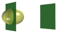
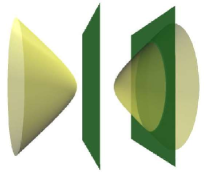
Figure 14: The two cases in the proof of Theorem 14 where the QSIC has one real conic and one imaginary conic.

When $\varepsilon_{1}$ and $\varepsilon_{2}$ have opposite signs, the index sequence is $\langle 2||2\rangle$. In this case the quadric ${\mathcal{A}^{\prime}}$ is a one-sheet hyperboloid and ${\mathcal{B}^{\prime}}$ comprises two planes intersecting ${\mathcal{A}^{\prime}}$ in an ellipse and a hyperbola in the affine realization shown in Figure 15. Since the ellipse intersects the hyperbola at its two branches, any real plane in $\mathbb{PR}^{3}$ intersects at least one of the two conics.

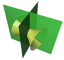
Figure 15: The case of QSIC having two real conics intersecting in two real points.

Now consider case ($ii$) of $a=0$. We transform the matrices $A^{\prime}$ and $B^{\prime}$ into the following forms,

$$A^{\prime}={\rm diag}\left(\;\left(\begin{array}[]{cc}0&1\\ 1&0\end{array}\right),\;\varepsilon_{1},\;\varepsilon_{2}\;\right),\;\;{\rm and}\;\;B^{\prime}={\rm diag}(-b,\;b,\;0,\;0\;).$$

The quadric ${\mathcal{B}^{\prime}}$ comprises of two planes. When $\varepsilon_{1}\varepsilon_{2}>0$, the only possible index sequence is $\langle 1||3\rangle$ (or its equivalent form $\langle 3||1\rangle$), the quadric ${\mathcal{A}^{\prime}}$ is a two-sheet hyperboloid, and the QSIC has one real and one imaginary conic, as shown in Figure 17.

When $\varepsilon_{1}\varepsilon_{2}<0$, the only possible index sequence is $\langle 2||2\rangle$, the quadric ${\mathcal{A}^{\prime}}$ is a one-sheet hyperboloid, and the QSIC has two real conics intersecting in two real points as shown in Figure 17. Again, as in case ($i$) where the index sequence is $\langle 2||2\rangle$, the two conic components of the QSIC cannot be both ellipses in any affine realization of ${\mathbb{PR}}^{3}$. This completes the proof of Theorem 14.

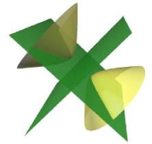
Figure 16: The case of the QSIC having two conics, one real and one imaginary.

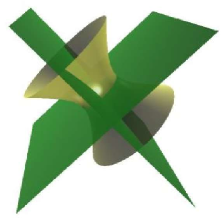
Figure 17: The case of the QSIC having two real conics intersecting in two real points.

Proof of Theorem 15 Clearly, all the roots of $f(\lambda)=0$ are necessarily real in this case. Wlog, we may assume the triple root $\lambda_{0}$ to be zero. Then, by Theorem 1, the canonical matrix forms of the given quadrics are

$$A^{\prime}={\rm diag}(\varepsilon_{1},\;\varepsilon_{2},\;\varepsilon_{3},\;\varepsilon_{4}\;),\;\;\;\;B^{\prime}={\rm diag}(\varepsilon_{1}\lambda_{1},\;0,\;0,\;0\;).$$

Setting $\lambda_{1}A^{\prime}-B^{\prime}$ to be $A^{\prime}$ and then $\varepsilon_{1}B^{\prime}$ to be $B^{\prime}$, we obtain

$$A^{\prime}={\rm diag}(0,\;\varepsilon_{2}\lambda_{1},\;\varepsilon_{3}\lambda_{1},\;\varepsilon_{4}\lambda_{1}\;),\;\;B^{\prime}={\rm diag}(\lambda_{1},\;0,\;0,\;0\;).$$

The quadric ${\mathcal{A}^{\prime}}$ is a cylinder (real or imaginary) with the $x$-axis being its central axis, while the quadric ${\mathcal{B}^{\prime}}$ is a plane counted twice. Thus the QSIC is a conic counted twice, real or imaginary.

When $\varepsilon_{2}$, $\varepsilon_{3}$ and $\varepsilon_{4}$ have different signs, the only possible index sequence is $\langle 1|||2|3\rangle$ (or its equivalent form $\langle 3|||2|1\rangle$). In this case ${\mathcal{A}^{\prime}}$ is real, and the QSIC is a real conic counted twice. When $\varepsilon_{2}$, $\varepsilon_{3}$ ad $\varepsilon_{4}$ have the same sign, the only possible index sequence is $\langle 0|||3|4\rangle$ (or its equivalent form $\langle 3|||0|1\rangle$). In this case ${\mathcal{A}^{\prime}}$ is imaginary, and the QSIC is an imaginary conic counted twice. This completes the proof of Theorem 15.

Proof of Theorem 16 The two roots of $f(\lambda)=0$ are necessarily real. Let $\lambda_{0}$ denote the triple root and $\lambda_{1}$ denote the simple root. Wlog, we assume $\lambda_{0}=0$ and $\lambda_{1}>0$. By Theorem 1, the canonical matrices of the two given quadric are

$$A^{\prime}=\left(\begin{array}[]{cccc}0&\varepsilon_{1}&\\ \varepsilon_{1}&0\\ &&\varepsilon_{2}&\\ &&&\varepsilon_{3}\end{array}\right),\;\;B^{\prime}=\left(\begin{array}[]{cccc}0&&&\\ &\varepsilon_{1}&&\\ &&0&\\ &&&\varepsilon_{3}\lambda_{1}\\ \end{array}\right).$$

Since the index jump at a root of Jordan block of size $2\times 2$ is 0, the index jump at the triple root is $\pm 1$. It is then easy to see that the only possible index sequence is $\langle 1{\wr\wr}|2|3\rangle$ (or its equivalents). Thus, we have $\varepsilon_{2}=1$, $\varepsilon_{3}=1$.

The quadric ${\mathcal{A}^{\prime}}$, as $2\,\varepsilon_{1}\,y+z^{2}+w^{2}=0$, passes through the origin $(1,0,0,0)^{T}$ and its tangent plane at this point is $y=0$. The quadric ${\mathcal{B}^{\prime}}$: $\varepsilon_{1}\,y^{2}+\lambda_{1}\,w^{2}=0$, comprises two planes intersecting at the line $(y=0,w=0)$, which touches the quadric ${\mathcal{A}^{\prime}}$ at the point $(1,0,0,0)^{T}$. Since the tangent plane $y=0$ of $\mathcal{A}$ at $(1,0,0,0)^{T}$ is different from either of these two planes, the QSIC comprises two conics that are tangent to each other at the real point $(1,0,0,0)^{T}$.

If the $\varepsilon_{1}=1$, ${\mathcal{B}^{\prime}}$ consists of two imaginary planes, so the QSIC consists of two imaginary conics. In this case, the number of positive eigenvalues of $-B^{\prime}$ is 0, and the index sequence therefore becomes $\langle 1{\wr\wr}_{+}|2|3\rangle$. If $\varepsilon_{1}=-1$, ${\mathcal{B}^{\prime}}$ consists of two real planes, so the QSIC consists of two real conics. In this case, the number of positive eigenvalues of $-B^{\prime}$ is 1, and the index sequence therefore becomes $\langle 1{\wr\wr}_{-}|2|3\rangle$. This completes the proof of Theorem 16.

Proof of Theorem 17 The two double roots of $f(\lambda)=0$ are necessarily real. Up to equivalence relations, the only possibilities for the index sequences are $\langle 2{\wr\wr}_{-}2||2\rangle$, $\langle 1{\wr\wr}_{-}1||3\rangle$ and $\langle 1{\wr\wr}_{+}1||3\rangle$. Note that $\langle 2{\wr\wr}_{-}2||2\rangle$ is equivalent to $\langle 2{\wr\wr}_{+}2||2\rangle$. Let $\lambda_{1}$ denote the root associated with the $2\times 2$ Jordan block, and let $\lambda_{2}$ denote the other root. By setting $B-\lambda_{1}\,A$ to $B$, we may assume $\lambda_{1}=0$. Let $\lambda_{2}$ denote the other double root; wlog, assume $\lambda_{2}>0$.

Then the canonical forms of the two quadrics are

$$A^{\prime}={\rm diag}\left(\;\left(\begin{array}[]{cc}0&\varepsilon_{1}\\ \varepsilon_{1}&0\end{array}\right),\;\varepsilon_{2},\;\varepsilon_{3}\;\right),\;\;B^{\prime}={\rm diag}\left(\left(\begin{array}[]{cc}0&0\\ 0&\varepsilon_{1}\end{array}\right),\;\varepsilon_{2}\lambda_{2},\;\varepsilon_{3}\lambda_{2}\;\right).$$ (17)

Due to the sign change rules (see Section 2.5), for the index sequence $\langle 2{\wr\wr}_{-}2||2\rangle$, we have $\varepsilon_{2}\varepsilon_{3}<0$. For the index sequences $\langle 1{\wr\wr}_{-}1||3\rangle$ and $\langle 1{\wr\wr}_{+}1||3\rangle$, we have $\varepsilon_{2}=\varepsilon_{3}=1$. Below we discuss these two cases: ($i$) $\varepsilon_{2}\varepsilon_{3}<0$; and ($ii$) $\varepsilon_{2}=\varepsilon_{3}=1$.

In case ($i$) of $\varepsilon_{2}\varepsilon_{3}<0$, setting $\varepsilon_{1}\lambda_{2}A^{\prime}-\varepsilon_{1}B^{\prime}$ to $\bar{A}$ and setting $B^{\prime}$ to $\bar{B}$, we obtain

$$\bar{A}={\rm diag}\left(\;\left(\begin{array}[]{cc}0&\lambda_{2}\\ \lambda_{2}&-1\end{array}\right),\;0,\;0\;\right),\;\;\bar{B}={\rm diag}\left(\;\left(\begin{array}[]{cccc}0&0\\ 0&\varepsilon_{1}\end{array}\right),\;\varepsilon_{2}\lambda_{2},\;\varepsilon_{3}\lambda_{2}\;\right),$$

Then the quadric $\bar{\mathcal{A}}$ consists of two planes $y=0$ and $y=2\lambda_{2}x$. The quadric $\bar{\mathcal{B}}$ is a real cylinder with the $x$-axis as its central axis. Clearly, $\bar{\mathcal{B}}$ intersects $y=0$ in two real lines, denoted by $\ell_{1}$ and $\ell_{2}$, on the planes $z=\pm 1$. These two lines intersect at the point $(1,0,0,0)^{T}$. The quadric $\bar{\mathcal{B}}$ also intersects the plane $y=2\lambda_{2}x$ in a real conic, which intersects the two lines $\ell_{1,2}$ in two distinct real points. This completes the proof of item 1.

In case ($ii$) of $\varepsilon_{2}=\varepsilon_{3}=1$, ${\rm Id}(A^{\prime})=3$, and the index jump at the root $\lambda_{2}$ is $2$. Below we distinguish two subcases: ($ii$-$a$) $\varepsilon_{1}<0$; and ($ii$-$b$) $\varepsilon_{1}>0$.

In subcase ($ii$-$a$) of $\varepsilon_{1}<0$, the index sequence is $\langle 1{\wr\wr}_{-}1||3\rangle$. The quadric ${\mathcal{B}^{\prime}}$ is a real hyperbolic cylinder with $x$-axis as central axis and symmetric with the plane $y=0$. Therefore it intersects the plane $y=0$ in two imaginary lines and intersects the plane $y=2\lambda_{2}x$ in a real conic. The two lines intersect at the point $(1,0,0,0)^{T}$. This completes the proof of item 2.

In subcase ($ii$-$b$) of $\varepsilon_{1}>0$, the index sequence is $\langle 1{\wr\wr}_{+}1||3\rangle$. The quadric ${\mathcal{B}^{\prime}}$ is an imaginary cylinder; thus it intersects the quadric ${\mathcal{A}^{\prime}}$ in an imaginary conic and two complex conjugate lines; these two lines intersect at the real point $(1,0,0,0)^{T}$. This completes the proof of item 3, and hence, Theorem 17.

Proof of Theorem 18 Wlog, we may assume the quadruple root, denoted by $\lambda_{1}$, to be 0. Then, by Theorem 1, the canonical form of the two quadrics are

$$A^{\prime}=\left(\begin{array}[]{cccc}0&&\varepsilon_{1}&\\ &\varepsilon_{1}&&\\ \varepsilon_{1}&&0&\\ &&&\varepsilon_{2}\end{array}\right),\;\;B^{\prime}=\left(\begin{array}[]{cccc}0&&&\\ &0&\varepsilon_{1}&\\ &\varepsilon_{1}&0&\\ &&&0\end{array}\right).$$ (18)

The quadric ${\mathcal{B}^{\prime}}$ comprises two planes $y=0$ and $z=0$. The plane $y=0$ intersects the quadric ${\mathcal{A}^{\prime}}$ along a real conic $xz=-{\varepsilon_{2}/\varepsilon_{1}w^{2}}$, denoted as ${\mathcal{C}}$. The plane $z=0$ intersects ${\mathcal{A}^{\prime}}$ in two lines, defined by the intersection of $z=0$ and $y^{2}=-{\varepsilon_{2}/\varepsilon_{1}}w^{2}$. If ${\varepsilon_{2}/\varepsilon_{1}}=-1$, the two lines are real; if ${\varepsilon_{2}/\varepsilon_{1}}=1$, the two lines are imaginary. In both cases, the two lines intersect the conic ${\mathcal{C}}$ at the real point $(1,0,0,0)^{T}$.

On the other hand, when ${\varepsilon_{2}/\varepsilon_{1}}=-1$, we have index($A^{\prime}$)= 2 and the index jump of ${\rm Id}(\lambda A-B)$ at the root $\lambda_{1}=0$ is 0. Therefore, the index sequence is $\langle 2{\wr\wr}{\wr}_{-}|2\rangle$ or its equivalent form $\langle 2{\wr\wr}{\wr}_{+}|2\rangle$. When ${\varepsilon_{2}/\varepsilon_{1}}=1$, we have $\mathrm{index}(A^{\prime})=1$ or $3$, and the index jump of ${\rm Id}(\lambda A-B)$ at $\lambda_{1}=0$ is $\pm 2$. Therefore, the index sequence of the pencil is $\langle 1{\wr\wr}{\wr}|3\rangle$. This completes the proof of Theorem 18.

Proof of Theorem 19 Let the two roots be $\lambda_{1}$ and $\lambda_{2}$. By setting $B^{\prime}=B-\lambda_{1}A$, we may assume $\lambda_{1}=0$. By Theorem 1, the canonical form of the two quadrics are

$$A^{\prime}={\rm diag}(\varepsilon_{1},\;\varepsilon_{2},\;\varepsilon_{3},\;\varepsilon_{4}),\;\;B^{\prime}={\rm diag}(0,\;0,\;\varepsilon_{3}\lambda_{2},\;\varepsilon_{4}\lambda_{2}\;).$$ (19)

Setting $\lambda_{2}A^{\prime}-B^{\prime}$ to be $A^{\prime}$, we obtain

$$A^{\prime}={\rm diag}(\varepsilon_{1}\lambda_{2},\;\varepsilon_{2}\lambda_{2},\;0\;0),\;\;B^{\prime}={\rm diag}(0,\;0,\;\varepsilon_{3}\lambda_{2},\;\varepsilon_{4}\lambda_{2}\;).$$ (20)

We consider the following three cases: ($i$) $\varepsilon_{1}\varepsilon_{2}<0$ and $\varepsilon_{3}\varepsilon_{4}<0$; ($ii$) $\varepsilon_{1}\varepsilon_{2}>0$ and $\varepsilon_{3}\varepsilon_{4}>0$; and ($iii$) $(\varepsilon_{1}\varepsilon_{2})(\varepsilon_{3}\varepsilon_{4})<0$.

In case ($i$), the index jumps at $\lambda_{1}$ and $\lambda_{2}$ are both $0$. Hence, the only possible index sequence is $\langle 2||2||2\rangle$. In this case, each of ${\mathcal{A}^{\prime}}$ and ${\mathcal{B}^{\prime}}$ consists of a pair of real planes intersecting at a real line. Since the two real lines on ${\mathcal{A}^{\prime}}$ and ${\mathcal{B}^{\prime}}$ do not intersect, the QSIC consists of four real lines forming a quadrangle. This quadrangle can be obtained from a tetrahedron (defined by the four planes of ${\mathcal{A}^{\prime}}$ and ${\mathcal{B}^{\prime}}$) by removing two of the six sides; the two removed sides are the intersecting line of the plane pair ${\mathcal{A}^{\prime}}$ and the intersecting line of the plane pair ${\mathcal{B}^{\prime}}$. This completes the proof of item 1.

In case ($ii$), the index jumps at $\lambda_{1}$ and $\lambda_{2}$ are both $\pm 2$. Hence, the only possible index sequence is $\langle 0||2||4\rangle$. In this case, each of ${\mathcal{A}^{\prime}}$ and ${\mathcal{B}^{\prime}}$ consists of a pair of complex conjugate planes intersecting at a real line. Since the two real lines on ${\mathcal{A}^{\prime}}$ and ${\mathcal{B}^{\prime}}$ do not intersect, the QSIC consists of four imaginary lines and has no real point. This completes the proof of item 2.

In case ($iii$), either $\varepsilon_{1}\varepsilon_{2}>0$ and $\varepsilon_{3}\varepsilon_{4}<0$ or $\varepsilon_{1}\varepsilon_{2}<0$ and $\varepsilon_{3}\varepsilon_{4}>0$. Thus the only possible index sequence is $\langle 1||1||3\rangle$ or its equivalent forms. At the same time, one of ${\mathcal{A}^{\prime}}$ and ${\mathcal{B}^{\prime}}$ is a pair of real planes and the other is pair of conjugate planes. Therefore, the QSIC consists two pairs of conjugate lines with each pair intersecting at a real point. This completes item 3, and hence, Theorem 19.

Proof of Theorem 20 By Theorem 1,

$$A^{\prime}={\rm diag}\left(\;\left(\begin{array}[]{cc}0&1\\ 1&0\end{array}\right),\;\left(\begin{array}[]{cc}0&1\\ 1&0\end{array}\right)\;\right),\;\;B^{\prime}={\rm diag}(-1,\;1,\;-1,\;1).$$

Then ${\mathcal{A}^{\prime}}$ is a hyperbolic paraboloid $xy+zw=0$ and ${\mathcal{B}^{\prime}}$ is a hyperboloid $-x^{2}+y^{2}-z^{2}+w^{2}=0$. It is easy to verify that the QSIC consists of the two non-intersecting real lines defined by ($x+w=0$, $y-z=0$) and ($x-w=0$, $y+z=0$), and two non-intersecting imaginary lines defined ($x-iz=0$, $y-iw=0$) and ($x+iz=0$, $y+iw=0$). In this case, since ${f}(\lambda)=0$ has no real root, the index sequence is $\langle 2\rangle$. This completes the proof of Theorem 20.

Proof of Theorem 21 The quadruple root, denoted by $\lambda_{1}$, of $f(\lambda)=0$ is necessarily real. Wlog, we may assume $\lambda_{1}=0$. By Theorem 1, the canonical form of the two given quadrics are

$$A^{\prime}={\rm diag}\left(\;\left(\begin{array}[]{cc}&\varepsilon_{1}\\ \varepsilon_{1}&\end{array}\right),\;\varepsilon_{2},\;\varepsilon_{3}\right),\;\;B^{\prime}={\rm diag}(0,\;\varepsilon_{1},\;0,\;0\;).$$

The quadric ${\mathcal{B}^{\prime}}$ is a pair of the identical real plane $y=0$. Substituting $y^{2}=0$ in the the quadric ${\mathcal{A}^{\prime}}$, we find that the QSIC is the intersection between $y^{2}=0$ and the pair of planes $z^{2}=-\varepsilon_{3}/\varepsilon_{2}w^{2}$. Clearly, the QSIC comprises two intersecting real lines, counted twice, if $\varepsilon_{2}\varepsilon_{3}=-1$, or a pair of conjugate lines, counted twice, if $\varepsilon_{2}\varepsilon_{3}=1$.

Clearly, the index jump of ${\rm Id}(\lambda A^{\prime}-B^{\prime})$ at $\lambda_{1}=0$ is 0 or $\pm 2$. When $\varepsilon_{3}/\varepsilon_{2}=-1$, $\det(A)=-\varepsilon_{2}\varepsilon_{3}>0$, therefore ${\rm index}(A^{\prime})$ is 0, 2 or 4. It follows that the index sequence is $\langle 2{\wr\wr}_{-}||2\rangle$ or its equivalent form $\langle 2{\wr\wr}_{+}||2\rangle$. When $\varepsilon_{3}/\varepsilon_{2}=1$, $\det(A)=-\varepsilon_{2}\varepsilon_{3}<0$, therefore ${\rm index}(A^{\prime})$ is 1 or 3. It follows that the index sequence is $\langle 1{\wr\wr}_{-}||3\rangle$ or its equivalent form $\langle 1{\wr\wr}_{+}||3\rangle$. This completes the proof of Theorem 21.

Proof of Theorem 22 The quadruple root of $f(\lambda)=0$ is necessarily real, and may be assume to be $0$. Since the index jump at a real root with a $2\times 2$ Jordan block is 0, the index sequence is of the form $\langle 2\widehat{\wr\wr}\widehat{\wr\wr}2\rangle$. By Theorem 1, the canonical form of the two quadrics are

$$A^{\prime}={\rm diag}\left(\left(\begin{array}[]{cc}0&\varepsilon_{1}\\ \varepsilon_{1}&0\end{array}\right),\;\left(\begin{array}[]{cc}&\varepsilon_{2}\\ \varepsilon_{2}&\end{array}\right)\;\right),\;\;\;B^{\prime}={\rm diag}(0,\;\varepsilon_{1},\;0,\;\varepsilon_{2}\;).$$

The quadric ${\mathcal{A}^{\prime}}$ is the hyperbolic paraboloid

$$\varepsilon_{1}xy+\varepsilon_{2}zw=0,$$

and ${\mathcal{B}^{\prime}}$ is a pair of planes

$$\varepsilon_{1}y^{2}+\varepsilon_{2}w^{2}=0.$$

When $\varepsilon_{1}\varepsilon_{2}=1$, the index sequence is $\langle 2{\wr\wr}_{-}{\wr\wr}_{-}2\rangle$ or its equivalent form $\langle 2{\wr\wr}_{+}{\wr\wr}_{+}2\rangle$. In this case ${\mathcal{B}^{\prime}}$ comprises two conjugate planes $y+iw=0$ and $y-iw=0$, which intersects ${\mathcal{A}^{\prime}}$ in the real double line ($y=0$, $w=0$) and two non-intersecting imaginary lines ($x-iz=0$, $y-iw=0$) and ($x+iz=0$, $y+iw=0$).

When $\varepsilon_{1}\varepsilon_{2}=-1$, the index sequence is $\langle 2{\wr\wr}_{-}{\wr\wr}_{+}2\rangle$ or its equivalent form $\langle 2{\wr\wr}_{+}{\wr\wr}_{-}2\rangle$. In this case ${\mathcal{B}^{\prime}}$ comprises two real planes $y-w=0$ and $y+w=0$, which intersects ${\mathcal{A}^{\prime}}$ in the real double line ($y=0$, $w=0$) and two non-intersecting real lines ($x-z=0$, $y-w=0$) and ($x+z=0$, $y+w=0$).

This completes the proof of Theorem 22.

References

Abhyankar (1990)S.S. Abhyankar 1990.
Algebraic Geometry for Scientists and Engineers.
American Mathematical Society, Providence, R. I.
Basu et al. (2003)S. Basu, R. PollackandM.-F. Roy 2003.
Algorithms in Real Algebraic Geometry.
Springer-Verlag, Berlin.
Berberich
et al. (2005)E. Berberich, M.
Hemmer, L. Kettner, E. SchömerandN.
Wolpert 2005. An exact, complete and efficient implementation for
computing planar maps of quadric intersection curves, Proc. of
ACM Symposium on Computational Geometry 2005, 99–106.
Bromwich (1906)T.J. Bromwich 1906.
Quadratic forms and their classification by means of
invariant-factors, Cambridge Tracts in Mathematics and
Mathematical Physics, no. 3.
Chionh et al. (1991)E. Chionh, R.N. Goldman, andJ. Miller 1991.
Using multivariate resultants to find the intersection of
three quadric surfaces.
ACM Transactions on Graphics 10, 378–400.
Dupont (2004)L. Dupont 2004.
Paramétrage quasi-optimal de
l’intersection de deux
quadriques : théorie, algorithme et implantation.
Thèse d’université, Université Nancy II.
(7)
J.A. Dieudonné.
Sur la réduction canonique des couples de matrices.
Bull. Soc. Math. France, 74:130–146, 1946.
Dupont et al. (2003)L. Dupont, D. Lazard, S. Lazard, andS.
Petitjean 2003.
Near optimal parameterization of the
intersection of quadrics.
Proc. of the Nineteenth
Annual Symposium on Computational Geometry, 246–255.
Dupont et al. (2005)L. Dupont, D. Lazard, S. Lazard, andS.
Petitjean 2005.
Near optimial parameterization of the intersection of quadrics,
II. Classification of pencils,
Rapport de Recherche INRIA, No. 2668.
Emiris et al. (2004)Emiris, Z. Ioannis, andE. P.
Tsigaridas 2004.
Computing with real algebraic numbers of
small degree.
Proc. of ESA, 2003, Springer Verlag, Berlin.
Finsler (1937)P. Finsler 1937.
Uber das Vorkommen definiter und semidefiniter formen in scharen
quadratischer formen.
Comment. Math.
Helv.,9:188–192.
Farouki et al. (1989)R.T. Farouki, C.A. NeffandM.A. O’Connor
1989.
Automatic parsing of degenerate quadric-surface
intersections.
ACM Transactions on Graphics8, 174–203.
Geismann et al. (2001)N. Geismann, M. Hemmer, andE. Schoemer
2001.
Computing a 3-dimensional cell in an arrangement of
quadrics: exactly and actually!
Proc. of ACM
symposium on Computational Geometry, 264–273.
Golub and van Loan (1989)G. H. GolubandC. F. van Loan 1989.
Matrix Computations.
Johns Hopkins University Press, Baltimore, MD, 2nd edition.
Killing (1872)W. Killing 1872.
Der Flächenbüschel zweiter Ordnung, Gustav
Schade, Berlin.
(16)
Peter Lancaster and Leiba Rodman.
Canonical forms for hermitian matrix pairs under strict equivalence
and congruence.
SIAM Rev., 47(3):407–443, 2005.
Lazard et al. (2004)S. Lazard, L.M. PeñarandaandS.
Petitjean 2004.
Intersecting quadrics: an efficient and
exact implementation.
Proc. of ACM symposium on
Computational Geometry, 419–428.
Levin (1976)J.Z. Levin 1976.
A parametric algorithm for drawing pictures of solid objects
composed of quadrics.
Communications of the ACM10, 555–563.
Levin (1979)J.Z. Levin 1979.
Mathematical models for determining the intersection of quadric
surfaces.
Comput. Graph. Image Process57,
73–87.
Lin and Ng (1995)X. LinandT. Ng 1995.
“Contact
detection algorithms for three-dimensional ellipsoids in discrete
element modeling.”
International Journal for
Numerical and Analytical Methods in Geomechanics19,
653–659.
Miller (1987)J.R. Miller 1987.
Geometric approaches to nonplanar quadric surface intersection
curves.
ACM Transactions on Graphics6, 274–307.
Miller and Goldman (1995)J.R. MillerandR.N. Goldman 1995.
Geometric algorithms for detecting and calculating all conic
sections in the intersection of any two natural quadric surfaces.
Graphical Models and Image Processing57, 55–66.
Mourrain et al. (2005)B. Mourrain, F. Rouillier, andM.-F. Roy
2005.
Bernstein’s basis and real root isolation.
Combinatorial and Computational Geometry (ed. J.E.
Goodman, J.E. and E. Welzl), Mathematical Sciences Research
Institute Publications. Cambridge University Press.
Mourrain et al. (2005)B. Mourrain, J.P. TécourtandM.
Teillaud 2005.
On the computation of an arrangement of
quadrics in 3D.
Computational Geometry30, 145–164.
(25)
P. Muth.
Über reele Äquivalenz von Scharen reeler Quadratischer Formen.
Crelle’s Journal, 128:302–343, 1905.
Ocken et al. (1987)S. Ocken, Jacob T. SchwartzandM. Sharir
1987.
Precise implementation of CAD primitives using
rational parametrizations of standard surfaces.
Planning, Geometry, and Complexity of Robot Motion, Ablex
Publishing Corporation, 245–266.
Rimon and Boyd (1997)E. RimonandS.P. Boyd 1997.
Obstacle
collision detection using best ellipsoid fit.
Journal
of Intelligent and Robotic Systems18, 105–126.
Perram et al. (1996)J. Perram, J. Rasmussen, E. PrastaardandJ. Lebowitz 1996.
“Ellipsoids contact potential: theory and relation to overlap potentials. ”
Physical Review E, 6, 6565–6572.
Sarraga (1983)R.F. Sarraga 1983.
Algebraic methods for intersections of quadric surfaces in
GMSOLID.
Computer Vision, Graphics and Image
Processing2, 222–238.
Shene and Johnstone (1994)C.K. SheneandJ.K. Johnstone 1994.
On the lower degree intersections of two natural quadrics.
ACM Transactions on Graphics4, 400–424.
Sieradski (1992)A. J. Sieradski 1992.
An Introduction to Topology and Homotopy, PWS-KENT Publishing Company, Boston.
Sommerville (1947)D. Sommerville 1947.
Analytical Geometry of
Three Dimensions, Cambridge University Press.
Staude (1914)O. Staude 1914.
Flächen 2. Ordnung und ihre Systeme
und Durchdringungskurven,
Encyklopädie der Mathematischen Wissenschaften, Volume III.C.2,
eds. W. F. Meyer and H. Mohrmann, Published by B. G. Teubner,
Leipzig, 161-256.
(34)
R. C. Thompson.
Pencils of complex and real symmetric and skew matrices.
Linear Algebra Appl., 147:323–371, 1991.
(35)
G. R. Trott.
On the canonical form of a non-singular pencil of hermitian matrices.
Amer. J. Math., 56:359–371, 1934.
Tu et al. (2002)C. Tu, W. WangandJ.Y. Wang 2002.
Classifying the morphology of the nonsingular intersection curves
of two quadric surfaces.
Proceedings of Geometric
Modeling and Processing, Tokyo, 23–32.
Tu et al. (2005)C. Tu, W. Wang, B. MourrainandJ.Y.
Wang 2002.