A Web-based Tool Combining Different Type Analyses

Abstract

There are various kinds of type analysis of logic programs. These include for example inference of types that describe an over-approximation of the success set of a program, inference of well-typings, and abstractions based on given types. Analyses can be descriptive or prescriptive or a mixture of both, and they can be goal-dependent or goal-independent. We describe a prototype tool that can be accessed from a web browser, allowing various type analyses to be run. The first goal of the tool is to allow the analysis results to be examined conveniently by clicking on points in the original program clauses, and to highlight ill-typed program constructs, empty types or other type anomalies. Secondly the tool allows combination of the various styles of analysis. For example, a descriptive regular type can be automatically inferred for a given program, and then that type can be used to generate the minimal “domain model” of the program with respect to the corresponding pre-interpretation, which can give more precise information than the original descriptive type.

1 Introduction

Type analysis has a long history in logic programming, going back to [Bruynooghe82a, Horiuchi-Kanamori, Mishra, Yardeni-Shapiro]. Roughly speaking we can divide the field into descriptive typing and prescriptive typing. In the former, we start with an untyped program and infer a set of type rules describing the terms that can appear in each argument position, automatically inventing types in the process. In the latter, we start from a program and some given types as well as possibly type signatures for the predicates, and infer types for the variables or other program points in the program.

Using a simple example, let us review the different approaches to type analysis. The descriptive approaches can be split into those that infer over-approximations, and those that compute a well-typing. The difference can be seen in a simple program such as the append program. Using a descriptive over-approximation, we could obtain a type signature append(list,any,any) where the type list is automatically constructed and defined by the regular type rules list --> []; [any|list] where any is the type containing all terms. Note that the second and third arguments cannot be approximated more precisely than any because (a) the base case of the append program allows any terms in these arguments, so that for example append([],foo,foo) is a consequence of the program, and (b) because the abstraction is based on arguments rather than relations. This means that we cannot capture the fact that the second argument of the program is a list if and only if the third argument is also a list.

A well-typing [BruynoogheGH05] could infer a type signature append(list(X),list(X),list(X)), where list(X) is defined by the parametrised type rule list(X) --> []; [X|list(X)], or else simply append(list,list,list) where list is defined as above. This is not an over-approximation of the success-set of the program; for example append([],foo,foo) is not well-typed by this signature. However, it gives a well-typing to all uses of the append program that are in fact used to append lists.

Now consider an approach in which types are given. Given the types list and any as defined above, an abstraction can be automatically constructed in which each term is interpreted either as list or as nonlist, where nonlist is defined as the difference of any and list. (This is equivalent to a pre-interpretation over the domain {list, nonlist} [BoBD94, BoB94, Gallagher-Boulanger-Saglam-ILPS95].) Computing the least model with respect to this abstraction, we obtain a model {append(list,list,list), append(list,nonlist,nonlist)}. This is a relational over-approximation of the success set of the append program. It is more accurate than append(list,any,any); for example the atom append([],foo,[]) is allowed by append(list,any,any) but not by the model {append(list,list,list), append(list,nonlist,nonlist)}.

The combination of these styles has not been investigated much to our knowledge, but the possibilities seem interesting. For instance, well-typings can be found in time roughly linear in the program being analysed [BruynoogheGH05]. However, these are not safe approximations and cannot directly be used to find type errors. However, by using the inferred types prescriptively to compute an abstract model, we can find bugs such as predicates that have no solution in the model, or variables that cannot be assigned a non-empty type. Similarly, an analysis based on a domain of NFTAs (non-deterministic finite tree automata) can yield complex types that would be very hard for a programmer to write by hand. These types, when used in a prescriptive analysis, can capture deeper properties of the program under analysis than could be easily identified otherwise.

In Section 2 we summarise the different type analysis methods handled by the tool. Section 3 briefly describes the approach to goal-dependent analyses in a bottom-up, goal-independent analysis framework. Section 4 presents the approach to using descriptive types as input to prescriptive type analyses, in order to gain precision. Section 5 outlines the implementation of the tool and its web interface. Section 6 discusses some future work and gives a summary and conclusion.

2 Type Analysis Methods

The type analysis tool includes at present three main type analysis engines:

• Domain model: given a program and a regular type, the tool computes the least model with respect to the pre-interpretation derived from the type. A BDD-based solver can be optionally used to compute the model, giving greater scalability (at the cost of some pre-processing).

• Well-typing: given a program, the tool computes types and predicate signatures that are a well-typing for the program.

• NFTA: given a program, the tool computes a regular type (non-deterministic finite tree automaton) that represents an over-approximation of the least model of the program.

This is not by any means a complete set of type analysis tools. For instance, we did not include a type analysis tool using widening [Gallagher-deWaal-ICLP94, VanHentenryck-Cortesi-LeCharlier, VaucheretB02], or a polymorphic type analysis with explicit type union and intersection operations [Lu00]. These could be incorporated later, but we believe that the above tools are representative of the main styles of type analysis. These tools are all goal-independent but we have implemented goal-dependent analyses using query-answer transformations [Debray-Ramakrishnan-94, Gallagher-deWaal-LOPSTR92]. We review next the main aspects of each of these tools.

2.1 Domain Model

The analysis is based on given regular types. More details can be found in [Gallagher-Henriksen-ICLP04, Gallagher-Henriksen-Banda-2005]. A regular type $R$ can be viewed as a finite tree automaton (FTA) [Comon], in which a type rule say list --> []; [dynamic|list] is viewed as the tree automata transitions $[]\rightarrow{\it list}$ and $[{\it dynamic}|{\it list}]\rightarrow{\it list}$. Using a standard algorithm from tree automaton theory we can obtain an FTA $R^{\prime}$ that accepts exactly the same set of terms as $R$, but is bottom-up deterministic (a DFTA). Each rule of a DFTA is of the form $f(q_{1},\ldots,q_{n})\rightarrow q$ and there are no two terms with the same left hand side. This implies that each term is accepted by at most one state of $R^{\prime}$. Determinisation of an FTA with states $Q$ yields an FTA whose states are a subset of $2^{Q}$. A state $\{q_{1},\ldots,q_{k}\}$ in the DFTA accepts terms that are accepted by all of the states $q_{1},\ldots,q_{k}$ in the original FTA, and by no other states in $Q$. For instance, consider a matrix transpose program.

transpose(Xs,[]) :- nullrows(Xs).

transpose(Xs,[Y|Ys]) :- makerow(Xs,Y,Zs), transpose(Zs,Ys).

makerow([],[],[]).

makerow([[X|Xs]|Ys],[X|Xs1],[Xs|Zs]):- makerow(Ys,Xs1,Zs).

nullrows([]).

nullrows([[]|Ns]) :- nullrows(Ns).

As this program is intended to manipulate matrices of unknown type, we define the following types matrix, row and dynamic, expressed as an FTA.

[] -> matrix

[row|matrix] -> matrix

[] -> row

[dynamic|row] -> row

Our intention is to analyse the transpose program in order to discover whether the program’s arguments have the expected types. Note that the above FTA is not bottom-up deterministic since there are two transitions with left hand side equal to $[]$. Determinisation of this FTA together with the rules defining dynamic for the program’s signature, yields the following states and type rules (assuming that the signature is {cons/2, []/0, 0/0, s/1}).

[] -> {dynamic,matrix,row}

[{dynamic,matrix,row}|{dynamic,matrix,row}] -> {dynamic,matrix,row}

[{dynamic,row}|{dynamic,matrix,row}] -> {dynamic,matrix,row}

[{dynamic}|{dynamic,matrix,row}] -> {dynamic,row}

[_|{dynamic,row}] -> {dynamic,row}

[_|{dynamic}] -> {dynamic}

0 -> {dynamic}

s({dynamic}) -> {dynamic}

Note that in the determinised automaton the states are sets of states in the original FTA. These rules define an abstraction over the domain elements {{dynamic,matrix,row}, {dynamic,row}, {dynamic}}, which represent the following sets of terms.

• {dynamic,matrix,row}: the set of terms that are in all the types matrix, row and dynamic. {dynamic,matrix,row} is equivalent to matrix since matrix is a subset of both row and dynamic.

• {dynamic,row}: the set of terms that are in the types row and dynamic but not in matrix, that is, it is the set of lists whose elements are not all lists.

• {dynamic}: the set of terms that are in dynamic but not in the other types.

These three types are disjoint and complete; every term is in exactly one of these types. We can compute the minimal model of a program based on this DFTA (for details of the process see [Gallagher-Henriksen-ICLP04]). In the model of this program over the domain {{dynamic,matrix,row}, {dynamic,row}, {dynamic}} defined above, the transpose predicate has the model

transpose({dynamic,matrix,row},{dynamic,matrix,row})

indicating that it can only succeed with both arguments matrix. Figure 1 displays a screenshot of the tool, showing the transpose program, and the regular type defining matrix and row.

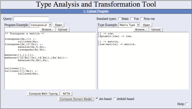
Figure 1: The main tool interface showing a program and type ready for analysis

Figure 2 shows the results of computing the domain model, for the transpose predicate. The model of the predicate appears when the mouse is moved over the symbol to the left of the head of a clause for transpose. Note that for brevity the domain elements are numbered and a key is given alongside the predicate’s model. Also, the type dynamic is omitted since it intersects with every other type, hence the type [] mentioned in Figure 2 is in fact the type {dynamic}. If any predicate has an empty model, then the heads of its clauses are highlighted in red.

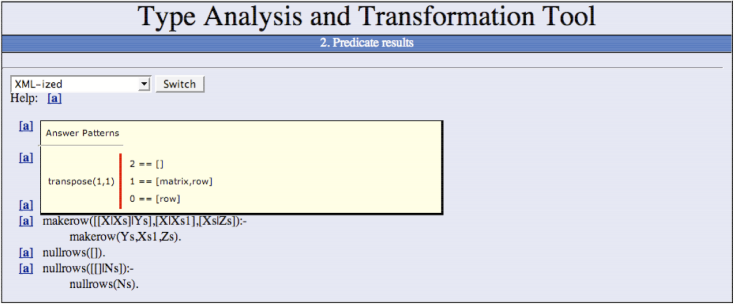
Figure 2: Displaying the model of the transpose predicate

2.1.1 Modes as regular types.

The type dynamic depends on the signature of the program. We call such types contextual types [GallagherPA05]. Other contextual types are those defining the set of grounds terms (called static) or non-variables terms (called nonvar). We assume that the signature contains some constant $VAR that does not appear in any program or query. The rules for contextual types are generated automatically by the system for the given program’s signature, and the user does not in fact see these rules at all. The rules defining static are all those of the form f(static,...,static) -> static for each function f in the signature apart from $VAR, while the rules defining nonvar are all rules of the form f(dynamic,...,dynamic) -> nonvar for each function f in the signature apart from $VAR. The rules for dynamic do include a rule $VAR -> dynamic, and thus the types static and nonvar are not identical to each other or to dynamic. A type var can also be defined using the single type rule $VAR -> var.

In the tool, the user can select one or more of the standard types static, nonvar and var and add them to the types to be used for analysis. (The type dynamic is always included automatically, to ensure that the types are complete).

The tool can thus be used for some classic mode analyses. By selecting the type static alone, the domain model computed represents the pos analysis [Marriott-Sondergaard-LOPLAS93]. Determinisation of the types static and dynamic results in two elements that represent the sets of ground and non-ground terms respectively. Similarly, selecting the type var (or nonvar) alone results in a freeness dependency analysis, distinguishing variable and non-variable terms. Combinations of given types such as list with static or nonvar allows the user to distinguish say, ground and non-ground lists, or distinguish lists from other non-variable terms.

2.2 Computing a Well-Typing

The well-typing tool computes a set of type rules and signatures and is described in detail in [BruynoogheGH05]. The result is displayed in the type window on the right hand side of the screen (see Figure 3).

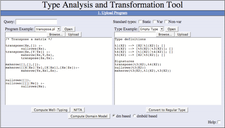
Figure 3: Displaying a well-typing of the transpose program

The types are parametric, and thus are more expressive than regular types. Note that the types inferred for the transpose program are in effect the types matrix and row defined earlier, except that there is a type parameter representing the type of the elements of the rows. Recall that a well-typing does not necessarily represent a safe approximation of the success set of the given program. It only gives types that consistently indicate the way in which the predicates are actually called in the program. As we will discuss in Section 4 the well-typing can be checked to see whether it is also a safe approximation. Note that there is some duplication in the types; for example t3 and t4 are renamings of each other, as are t1 and t5. In future work we intend to identify and remove such identical types, using the determinisation algorithm employed in the domain model tool to detect the redundancy.

2.3 Computing a Non-Deterministic Regular Type Approximation

The third analysis method is the computation of a non-deterministic finite tree automaton that over-approximates the least model of the given program. This method is described in [Gallagher-Puebla-02]. The generated types tend to be complex and difficult to read. The most interesting information is usually the emptiness of a type. As with the well-typing, the result is displayed in the type window, and can then be converted to a regular type and used to build a domain model. Conversion to regular type form in this case is simple, as the inferred types are already regular type rules. We just need to remove the rules defining the types of the predicates (which will be recomputed during the domain model construction).

3 Goal-Dependent Type Analysis

Transformations to allow goal-dependent analysis using a goal-independent analysis tool are well known [Debray-Ramakrishnan-94, Gallagher-deWaal-LOPSTR92], and have their origin in the “magic set” and “Alexander” methods from deductive databases[Bancilhon-Maier-Sagiv-Ullman]. The common feature of these transformations is the definition of “query predicates” corresponding to the program predicates. The variant we use in the tool constructs a separate query predicate for each body literal in the program. A similar transformation was described in [Gallagher-deWaal-LOPSTR92]. As the result of analysis of query-answer transformed programs can be hard to read, the tool displays the models of the query predicates at the corresponding body calls in the original program. An example is shown in Figure 4. When the mouse is moved over the symbol to the left of each body call, the query patterns for that call are displayed, along with a key to the determinised types, as before.

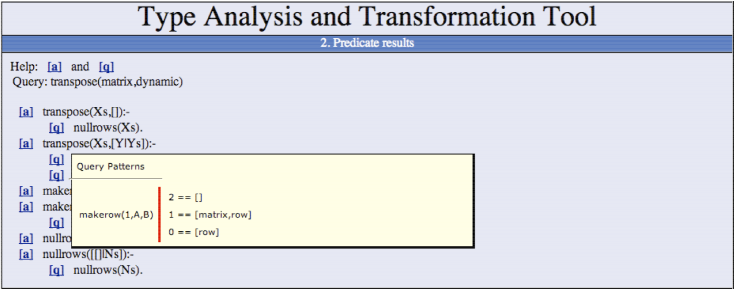
Figure 4: Displaying query patterns

4 From Descriptive to Prescriptive Types

As mentioned earlier, a descriptive analysis such as the well-typing or the NFTA analysis constructs types automatically. Apart from providing documentation about the program predicates, these types can be used for prescriptive analysis where types have to be provided. In [BruynoogheGH05] the types were used to generate type-based norms for termination analysis. In the present context, the inferred types can be input to the domain model tool. The main reason for doing this is to generate more precise information about failure and dead code in the program. Consider the naive reverse program. The well-typing analysis informs us that both arguments of reverse are lists, but we do not know whether this is a safe approximation.

A goal-independent NFTA analysis of the same program gives the information that the second argument of reverse is approximated by dynamic. By taking the result of either of these analyses and using it as the regular type in the domain model tool, we can verify that the second argument of reverse is indeed approximated by the type list. (We would get the type presented with some system-generated type name such as [] -> t1, [dynamic|t1] -> t1 which we would have to recognise as list. Recognition of standard regular types is already performed by the CiaoPP analysis tool [Hermenegildo-Bueno-Puebla-Lopez] and might be added to our tool in the future). This allows us to detect as ill-typed any call to reverse whose second argument is typed by a non-list.

As can be seen in Figure 3, the tool offers the possibility of using the inferred well-typings or NFTA analysis results to construct regular types. In the case of well-typing rules this just involves replacing the parameters by dynamic, which involves a loss of precision. The NFTA types can be used directly with minor syntactic changes. The regular types can then be used to build a domain model, as in Section 2.1.

NFTA types tend to be large and complex with much redundancy in the form of multiple occurrences of the same type with different names. So far, the most likely uses of NFTA analysis is to find useless clauses, dead-code, failing calls and such like. Determinisation and computation of a domain model can enhance the ability to search for such anomalies. An example is provided by the tokenring.pl program on the sample program menu. An NFTA analysis yields types, but every predicate has a non-empty type. If the derived types are converted to a regular type and a domain model is computed, then the fact that unsafe/1 has an empty type is detected. The BDD-based domain-model tool is required to get this result; the NFTA type rules are complex and the determinised automaton has 111 distinct states.

5 Features of the Implementation

The Type Analysis Toolkit consists of a back-end and a front-end. The back-end consists of the analysis programs themselves, and the front-end is a user friendly web-interface for those tools. There are obvious advantages of using a web-based interface; one of these is of course that anyone wishing to try the tool for himself can do so without having to install software on his own machine and dealing with possible incompatibilities in operating systems and so on. It is also intuitively easier to use a programming tool with a graphical interface, than having to e.g. read and decipher command line options.

5.1 Back-end

There are currently three tools in the back-end: the domain-model analyser, the polymorphic type analyser and the NFTA analysis tool - all written in Prolog. The particular Prolog system we are using is the Ciao Prolog Development System.

Initially the back-end tools were developed independently and were intended to be executed within a Prolog environment. They have been modified to allow them to be compiled into two separate command line tools. It is also possible to use the Ciao-shell environment for running the back-end tools from the command line. This method does not require compilation of the tools, but it comes with a performace penalty. Table 1 shows the analysis time for a few select programs; the append program, Leuschel & Massart’s model checker for CTL formulas [Leuschel-Massart-LOPSTR99], and the token ring program mentioned earlier in Section 4. The table compares a compiled version of the Domain Model (DM) program to a version of DM executed in the Ciao-shell environment. For larger programs the penalty of using Ciao-shell may be insignificant, but for smaller programs the compiled version is significantly faster.

Program	No. Clauses	Compiled DM	Ciao-shell DM
append.pl	2	0.4	3.7
tokenring.pl	20	0.9	3.5
ctl.pl	27	3.7	7.3

Table 1: This shows the analysis time in seconds for a few programs containing from 2 to 27 clauses

The tools were also modified to read their input and write output to files to simplify the development of the web interface. The output from the polymorphic type analyser is plain text. This output will be read by the domain model tool. The output from the domain model tool will be parsed by the front-end, so we decided to format this output in XML. The result from the domain model tool is a term containing the analysed program with clause heads and clause bodies annotated with the query and answer patterns. This term is not a syntactically correct Prolog program, and we have therefor written our own Prolog module to handle the output of terms in an XML structure. Tools for outputting and analysing Prolog code in XML exists [DBLP:conf/lpe/SeipelHH03], but at the moment we only need to separate clauses and calls from annotations when presenting the analysis results in HTML.

5.2 Front-end

The invoking of the back-end tools and the presentation of the analysis results are handled by the front-end. The front-end has two main parts; a page with a form to be filled in by the user, where the user uploads, types in or selects one of the supplied example programs and types, and a presentation page where the analysis results are displayed. The front-end is built on the Apache webserver, the PHP scripting language and libxml and libxslt. The design of the pages is inspired by other online analysers for logic programming developed in the context of the Framework 5 ASAP project.

The PHP language allows us to create dynamic pages in which, for example, buttons can be removed from the input-form if they do not apply to the current input given. It also enables us to execute the command line analysis tools and run the output through XSLT. XSLT provides a convenient way of automatically transforming the XML output into HTML that can be displayed in a browser. Depending on whether the analysis is performed with or without a query, the appropriate XSL style sheet is applied to the analyser output.

5.3 User’s guide

Using the analysis tools involves the following steps for the user:

1. Supplying a program for analysis

2. Inferring or supplying a set of types for analysis

3. If applicable, supply a typed goal for a goal dependent analysis

4. Selecting back-end tool for the analysis

A few example programs and types are available for a quick demonstration of the tool. Select the program tokenring.pl in the dropdown menu to the left and the type Ring Types in the dropdown menu to the right. In the query-field type unsafe(dynamic). Make sure the dm-based back-end is selected next to the Compute Domain Model button. Then click this button. Notice that the predicate unsafe has no answers, meaning no unsafe state can occur in the token ring.

5.3.1 Selection of Program and Analysis Method

An example of the input page is shown in Figure 1. On the left side of the screen the user can either paste in a program to be analysed, select one of the example programs or upload a local file containing a program. On the right side of the screen, the user can supply the type, again either from a local file, by selecting one of the provided type definitions or by typing directly into the panel. At the bottom of the screen are the options to either run the Polymorphic Type Analyser, the Domain Model Analyser or the NFTA analysis on the given program. In the case of the Domain Model, the Prolog implementation or the BDD-based tool bddbddb can be selected. If the Polymorphic Type Analyser or the NFTA analysis is used, the result is shown to the right. A new option to convert to regular type will appear.

5.3.2 Display of Analysis Results

An example of the output page is shown in Figure 2. The analysed program is shown annotated with answer patterns and if a query was supplied to the analysis, also a query pattern for the calls in the body of the program clauses.

Placing the mouse over either of the annotations will show a small window with the actual patterns.

Should a clause have an empty answer pattern it will be coloured red to indicate that it is dead code. If a query was given to the analyser, the code is considered dead with respect to that particular query pattern.

Calls in the body of a query having an empty call pattern are similarly highlighted in red. These are calls that are redundant; they and the calls to their right in the clause can safely be “sliced” from the program, since they are not invoked in the computation of the given query.

The Analysis Toolkit (called Tattoo – Type analysis and transformation tool – is available online - to try it out, visit the URL http://wagner.ruc.dk/Tattoo/.

6 Future Development

The current tool provides a platform for experimentation. The front end and the back end are cleanly separated and so further tools could be added to the back end with minimal modification of the front end. The use of XML also allows us to experiment with different ways of displaying the results to the user.

Analysis of large programs using complex types is likely to require powerful tools such as the BDD-based analysis tool described in [Gallagher-Henriksen-Banda-2005, bddbddb]. An option in the interface to use this tool rather than the Prolog implementation has been implemented, but only goal-independent analysis can be carried out with this tool currently.

So far our effort has been focussed on developing the tool and considering the best way to present the results to the user and allow the results of one tool to be input to another. The interface will continue to undergo development as more experience is gained. Evaluation of the tool is being carried out and we hope that its availability on the web will enable feedback to be obtained from a wider range of users.

Acknowledgements

We thank the ASAP project team (http://www.clip.dia.fi.upm.es/Projects/ASAP/) for collaboration during the development of the tools and the online ASAP tool interface which incorporates some of the type analysis tools described here.