Loop Calculus and Belief Propagation for $q$-ary Alphabet: Loop Tower

Abstract

Loop Calculus introduced in [1, 2] constitutes a new theoretical tool that explicitly expresses the symbol Maximum-A-Posteriori (MAP) solution of a general statistical inference problem via a solution of the Belief Propagation (BP) equations. This finding brought a new significance to the BP concept, which in the past was thought of as just a loop-free approximation. In this paper we continue a discussion of the Loop Calculus. We introduce an invariant formulation which allows to generalize the Loop Calculus approach to a q-are alphabet.

The manuscript is organized as follows. In Section I we introduce a new formulation of the Loop Calculus in terms of a set of gauge transformations that keep the partition function of the problem invariant. The full expression contains two terms referred to as the “ground state” and “excited states” contributions. The BP equations are interpreted as a special (BP) gauge fixing condition that emerges as a special orthogonality constraint between the ground and the excited states. Stated differently, it selects the generalized loop contributions as the only ones that survive among the excited states. In Section II we demonstrate how the invariant interpretation of the Loop Calculus, introduced in the Section I, allows a natural extension to the case of a general $q$-ary alphabet. This is achieved via a loop tower sequential construction. The ground level in the tower is exactly equivalent to assigning one color (out of $q$ available) to the “ground state” and considering all “excited” states to be colored in the remaining $(q-1)$ colors, according to the loop calculus rule. Sequentially, the second level in the tower corresponds to selecting a loop from the previous step, colored in $(q-1)$ colors, and repeating the same ground vs excited states partitioning procedure into one and the remaining $(q-2)$ colors, respectively. The construction proceeds until the complete set of $(q-1)$ levels in the loop tower (including the corresponding contributions to the partition function) is established. In Section III we discuss an ultimate relation between the loop calculus and the Bethe free energy variational approach of [3].

We start with defining a statistical inference problem using the so-called Forney-style graphical model formulation [4, 5]. The basic graph, ${C_{0}}=({\cal V}_{0},{\cal E}_{0})$, is described in terms of vertices, ${\cal V}_{0}=\{a\}$ and edges, ${\cal E}_{0}=\{(ab)\}$. Variables, associated with the edges, assume their values in a $q$-ary alphabet, $\sigma_{ab}=\sigma_{ba}=0,\cdots,(q-1)$. The probability of a given configuration of variables ${\bm{\sigma}}=\{\sigma_{ab}|(ab)\in{\cal E}_{0}\}$ on the entire graph is described by

$$p({\bm{\sigma}})=Z_{C_{0}}^{-1}\prod\limits_{a}f_{a}\left({\bm{\sigma}}_{a}\right),\quad Z_{C_{0}}=\sum_{\bm{\sigma}}\prod\limits_{a}f_{a}\left({\bm{\sigma}}_{a}\right),$$ (1)

where $Z_{C_{0}}$ is the normalization coefficient, also known as the partition function; $f_{a}({\bm{\sigma}}_{a})$ is an arbitrary positive function of the variables, ${\bm{\sigma}}_{a}\equiv\{\sigma_{ab}|b\in a,{\cal E}_{0}\}$, associated with all edges attached to vertex $a$. $b\in a$ (or conversely $a\in b$) indicates that the vertices $b$ and $a$ share an actual edge of the graph, $(ab)\in{\cal E}_{0}$. The marginal probabilities, e.g. associated with edges and vertices,

$$p_{a}({\bm{\sigma}}_{a})\equiv\sum_{{\bm{\sigma}}\setminus{\bm{\sigma}}_{a}}p({\bm{\sigma}}),\quad p_{ab}(\sigma_{ab})\equiv\sum_{{\bm{\sigma}}\setminus\sigma_{ab}}p({\bm{\sigma}}),$$ (2)

constitute what one normally needs to evaluate in order to solve a statistical inference problem. The marginal probabilities can be also expressed in terms of derivatives of the so-called equilibrium free energy, ${\cal F}_{C_{0}}=-\ln Z_{C_{0}}$, with respect to relevant parameters of the factor functions.

I Gauge-Invariant Formulation of Loop Calculus

Formally, loop calculus suggests an explicit decomposition of the partition function $Z_{C_{0}}$ in terms of a sum over certain loops on the graph ${C_{0}}$. Below we re-derive the loop calculus in more general terms compared to [1, 2].

We start with an observation that the partition function, $Z_{C_{0}}$, is invariant with respect to a group of linear gauge transformations of the factor functions

$$f_{a}({\bm{\sigma}}_{a}=(\sigma_{ab},\cdots))\to\sum_{\sigma^{\prime}_{ab}}G_{ab}\left(\sigma_{ab},\sigma^{\prime}_{ab}\right)f_{a}(\sigma^{\prime}_{ab},\cdots),$$ (3)

described by $\hat{G}=\{G_{ab}(\sigma_{ab},\sigma^{\prime}_{ab});(ab)\in{\cal E}_{0}\}$ provided the pairs of conjugated matrices $G_{ab}$ and $G_{ba}$ are related to each other by the special constraint

$$\sum_{\sigma_{ab}}G_{ab}(\sigma_{ab},\sigma^{\prime})G_{ba}(\sigma_{ab},\sigma^{\prime\prime})=\delta(\sigma^{\prime},\sigma^{\prime\prime}),$$ (4)

where $\delta(x,y)$ is $1$ if $x=y$ and $0$, otherwise. Except as prescribed by Eq. (4), the gauges are chosen independently at different edges of the graphs. This local freedom in selecting $\hat{G}$ is the key to our further analysis of the partition function, $Z_{C_{0}}$ now expressed as

$$Z_{C_{0}}=\sum\limits_{\bm{\sigma}}\prod_{a}\left(\sum\limits_{\bm{\sigma}^{\prime}_{a}}f_{a}({\bm{\sigma}}^{\prime}_{a})\prod\limits_{b\in a}G_{ab}(\sigma_{ab},\sigma^{\prime}_{ab})\right)$$

$$\equiv\sum\limits_{\bm{\sigma}}\bar{p}\{\hat{G}|{\bm{\sigma}}\}\equiv\mbox{Tr}\left(\bar{p}\{\hat{G}|{\bm{\sigma}}\}\right),$$ (5)

where $\sigma_{ab}=\sigma_{ba}$. We will refer to summation over all allowed configurations of ${\bm{\sigma}}$ in Eq. (5) as computing a graphic trace: a conventional trace can be considered as a special case of the graphic trace for a graph that consists of a single vertex and a single edge. Our next step in evaluation of Eq. (5) is fixing the gauges, which means imposing constraints on $\hat{G}$ in addition to Eq. (4).

It is convenient to distinguish a special term in the sum/trace over ${\bm{\sigma}}$ in Eq. (5) with all $\sigma_{ab}=0$. We will refer to this term as the ground or, alternatively, uncolored state (term), while all the other terms in the sum, which contain at least one edge with $\sigma_{ab}>0$, are called excited (colored) states. Obviously for a general gauge choice $\hat{G}$ all kinds of excited states, e.g. with only one edge being excited/colored, provide nonzero contributions to $Z$. Discussing individual terms in the $\sigma$-sum in Eq. (5) we call a vertex colored if at least one edge attached to it is excited/colored.

A BP-gauge corresponds to such a special choice of $\hat{G}$ that makes vanish any contribution in the $\sigma$-sum in Eq. (5) that has at least one vertex with only one attached colored edge. Stated differently a BP-gauge prohibits loose excited/colored edges at any vertex. Formally it is expressed as the following set of conditions

$$\sum\limits_{{\bm{\sigma}^{\prime}}_{a}}f_{a}({\bm{\sigma}}^{\prime})G^{(bp)}_{ab}(\sigma_{ab}\neq 0,\sigma^{\prime}_{ab})\prod\limits_{c\in a}^{c\neq b}G^{(bp)}_{ac}(0,\sigma^{\prime}_{ac})=0,$$ (6)

enforced independently at any vertex of the graph. Combined with the constraints (4), Eq. (6) can be re-stated in the vector form depending only on the ground state part of the gauges:

$$G^{(bp)}_{ba}(0,\sigma^{\prime}_{ab})=\rho_{a}^{-1}\sum\limits_{{\bm{\sigma}^{\prime}}_{a}\setminus\sigma^{\prime}_{ab}}f_{a}({\bm{\sigma}}^{\prime})\prod\limits_{c\in a}^{c\neq b}G^{(bp)}_{ac}(0,\sigma^{\prime}_{ac}).$$ (7)

with

$$\rho_{a}=\sum\limits_{{\bm{\sigma}^{\prime}}_{a}}f_{a}({\bm{\sigma}}^{\prime})\prod\limits_{c\in a}G^{(bp)}_{ac}(0,\sigma^{\prime}_{ac}).$$ (8)

We can alternatively derive Eq. (7) for BP gauges using a variational approach. To that end we introduce a functional

$${\cal Z}_{0}(\hat{\epsilon})\equiv\bar{p}\{G|{\bm{0}}\}=\prod_{a}\rho_{a}({\bm{\epsilon}}_{a}),$$ (9)

where $\epsilon_{ab}(\sigma_{ab})\equiv G_{ab}(0,\sigma_{ab})$, ${\bm{\epsilon}}_{a}\equiv\{\epsilon_{ab}|b\in a,{\cal V}_{0}\}$, $\hat{\epsilon}\equiv\{\epsilon_{ab}|(ab)\in{\cal E}_{0}\}$, and $\rho_{a}({\bm{\epsilon}}_{a})$ is given by Eq. (8) with $G^{(bp)}_{ac}(0)$ replaced by $\epsilon_{ac}$. The conditions for the stationary points of ${\cal F}_{0}\equiv-\ln{\cal Z}_{0}$ with respect to $\hat{\epsilon}$, under the additional condition, $\sum_{\sigma}G_{ab}(0,\sigma)G_{ba}(0,\sigma)=1$, recovers Eqs. (7). Note that the functional ${\cal F}_{0}(\hat{\epsilon})$ as well as the BP equations (7,8) possess some remaining irrelevant gauge freedom with respect to a set of transformations $\epsilon_{ab}\to\kappa_{ab}\epsilon_{ab}$ with $\kappa_{ab}\kappa_{ba}=1$. Stated differently, the BP equations fix only the relevant part of the gauge freedom. A connection between the functional ${\cal F}_{0}(\hat{\epsilon})$ and the variational Bethe free energy will be established in Section III.

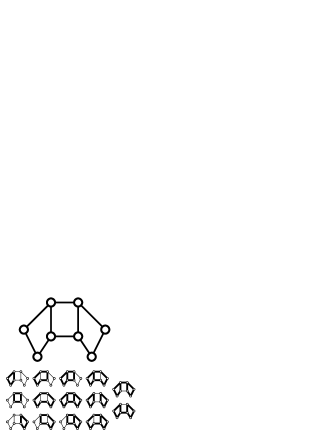
Figure 1: Example of a factor graph, ${\it C}_{0}$ with fourteen possible generalized loops, $\Omega({\it C}_{0})=\{{\it C}_{1}\}$, shown in bold on the bottom.

The conventional form of the BP equations, in terms of the “messages” $\eta_{ab}(\sigma_{ab})$,

$$\frac{\exp\left(\eta_{ab}^{(bp)}(\sigma_{ab})+\eta_{ba}^{(bp)}(\sigma_{ab})\right)}{\sum_{\sigma_{ab}}\exp\left(\eta_{ab}^{(bp)}(\sigma_{ab})+\eta_{ba}^{(bp)}(\sigma_{ab})\right)}$$

$$=\frac{\sum_{{\bm{\sigma}}_{a}\setminus\sigma_{ab}}f_{a}({\bm{\sigma}}_{a})\exp\left(\sum_{b\in a}\eta_{ab}^{(bp)}(\sigma_{ab})\right)}{\sum_{{\bm{\sigma}}_{a}}f_{a}({\bm{\sigma}}_{a})\exp\left(\sum_{b\in a}\eta_{ab}^{(bp)}(\sigma_{ab})\right)},$$ (10)

is recovered using the following parametrization

$$\epsilon_{ab}=G_{ab}(0,\sigma)=\frac{\exp\left(\eta_{ab}(\sigma)\right)}{\sqrt{\sum_{\sigma}\exp\left(\eta_{ab}(\sigma)+\eta_{ba}(\sigma)\right)}}.$$ (11)

Our discussion has been applied so far to the case of a general $q$-ary alphabet. We now turn to the simplest binary case $q=2$, where the ground state parametrization (11) unambiguously fixes the excited states: $G_{ab}(1,\sigma)=(1-2\sigma)G_{ba}(0,(\sigma-1)^{2})$. Substituting the latter expression and Eqs. (6,7) into Eq. (5) we arrive at the main formula of the loop calculus for the binary alphabet

$$Z_{C_{0}}\! = \!Z_{0;C_{0}}(1\!+\!\sum\limits_{C_{1}}\!\!r({C_{1}})),\ \ r(C_{1})\!\equiv\!Z_{0;C_{0}}^{-1}\bar{p}(G|{\bm{\sigma}}_{C_{1}}),$$

$$Z_{0;C_{0}} \equiv \bar{p}(G|{\bm{\sigma}}_{0}),\quad{\bm{\sigma}}_{0}\equiv\{\sigma_{ab}=0|\ \ (ab)\in{C_{0}}\},$$

$${\bm{\sigma}}_{C_{1}} \equiv \left\{\begin{array}[]{cc}\sigma_{ab}=1|&\quad(ab)\in{C_{1}}\\ \sigma_{ab}=0|&\quad(ab)\in{C_{0}}\setminus{C_{1}}.\end{array}\right\}.$$ (14)

where $\{{C_{1}}\}={\it\Omega}(C_{0})$ is the set of generalized loops on the graph, defined as subgraphs of ${C_{0}}$ without loose ends, i.e. with degree of connectivity at any vertex (within the subgraph) being two or larger.

Beliefs are defined here as substitutes for the exact marginal probabilities (2) truncated at the first, ground state, term

$$b^{(bp)}_{ab}(\sigma_{ab})=G_{ab}^{(bp)}(0,\sigma_{ab})G_{ba}^{(bp)}(0,\sigma_{ab}),$$ (15)

$$b^{(bp)}_{a}({\bm{\sigma}}_{a})=\frac{f_{a}({\bm{\sigma}}_{a})\prod_{b\in a}G_{ab}^{(bp)}(0,\sigma_{ab})}{\sum_{{\bm{\sigma}}_{a}}f_{a}({\bm{\sigma}}_{a})\prod_{b\in a}G_{ab}^{(bp)}(0,\sigma_{ab})}.$$ (16)

Then a single generalized loop contribution, $r_{C_{1}}$, is expressed in terms of the ground state beliefs in the following simple way

$$r(C_{1})\!\! = \!\!\!\frac{\prod\limits_{a\in{C_{1}}}\mu_{a}}{\prod\limits_{(ab)\in{C_{1}}}(1-m_{ab}^{2})},\ m_{ab}\!\equiv\!\sum\limits_{\sigma_{ab}}(1\!-\!2\sigma_{ab})b_{ab}^{(bp)}(\sigma_{ab}),$$

$$\mu_{a} \equiv \sum_{{\bm{\sigma}}_{a}}\left(\prod_{b\in a,{C_{1}}}(1\!-\!2\sigma_{ab}\!-\!m_{ab})\right)b_{a}^{(bp)}({\bm{\sigma}}_{a}).$$

The loop calculus construction for a simple example is illustrated schematically in Fig. 1.

II Loop Tower for $q$-ary alphabet

Turning to the general $q$-ary alphabet case we first notice that all considerations and formulas of the introduction and the first part of Section I, all the way up to Eq. (7), actually apply to the general $q$-ary case. Partitioning the sum/trace over ${\bm{\sigma}}$ in Eq. (5) into the ground-state term, with ${\bm{\sigma}}_{0}$, and the remaining excited-state terms $\{{\bm{\sigma}}\setminus{\bm{\sigma}}_{0}\}$, and emergence of the self-consistent set of equations for the ground state gauges (11) are important general features of the gauge fixing construction. Of course, all the preceding formulas should be understood in terms of the edge variables that assume values from $\{0,\cdots,q-1\}$. Generalization of Eq. (14) to a general $q$-ary alphabet reads

$$Z_{C_{0}}\!=\!Z_{0;{C_{0}}}\!+\!\!\!\!\!\sum\limits_{C_{1}\in{\it\Omega}({C_{0}})}\!\!\!\!\!\!\!Z_{C_{1}},\ Z_{C_{1}}\!=\!\sum_{{\bm{\sigma}}_{C_{1}}}\!{\bar{p}}(G^{(bp)}|{\bm{\sigma}}_{C_{1}}).$$ (17)

The additional summation over the colored/excited ${\bm{\sigma}}_{C_{1}}$ in Eq. (17) is a consequence of the fact that for $q>2$, ${\bm{\sigma}}_{C_{1}}$, is not fixed unambiguously, but rather represents summation over the reduced $(q-1)$-colors rich set, $1,\cdots,q-1$. The BP-gauges for the original graphical model are described by Eqs. (4,6). The set of excited states gets larger in the $q$-ary case and, consequently, there is a big freedom in selecting the orthogonal basis set of excited gauges. Selecting one such solution of Eqs. (4,6), $\{G_{ab;{C_{0}}}^{(bp)}(\sigma_{ab},\sigma^{\prime}_{ab});(ab)\in{C_{0}}\}$, and substituting it in Eq. (17) we find that $Z_{C_{1}}$ becomes the partition function of a reduced graphical model, defined on a subset $C_{1}\subset{C_{0}}$ of ${C_{0}}$,

$$Z_{C_{1}}=\sum_{{\bm{\sigma}}_{C_{1}}}\prod\limits_{a\in C_{1}}f_{1;a}({\bm{\sigma}}_{a;C_{1}}),\quad f_{1;a}({\bm{\sigma}}_{a;C_{1}})=$$ (18)

$$=\sum\limits_{{\bm{\sigma}}^{\prime}_{a}}f_{a}({\bm{\sigma}}^{\prime}_{a})\prod\limits_{b\in a,{C_{0}}}G_{ab;C_{0}}^{(bp)}(\sigma_{ab},\sigma^{\prime}_{ab})\prod\limits_{b\in a,{C_{0}}}^{b\notin C_{1}}\delta(\sigma_{ab},0).$$

Here ${\bm{\sigma}}_{a;C_{1}}$ is the vector constructed of $\sigma_{ab}$ with $b\in C_{1}$, with the components labeled by $\{1,\cdots,q-1\}$. $Z_{C_{1}}$ may be understood as a partition function of a reduced graphical model, defined on the graph $C_{1}$ in terms of a reduced (one element shorter) alphabet and with the factor functions $f_{1;a}$.

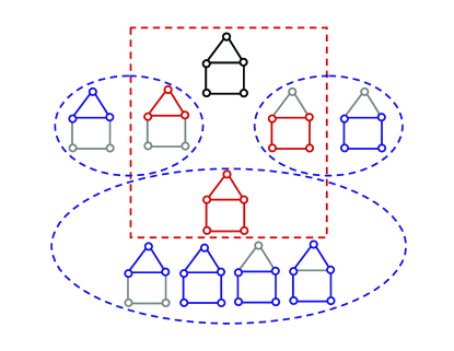
Figure 2: Example of a loop tower construction for three colors, $q=0,1,2$, shown in the Figure in black, red and blue respectively. First layer of the tower is bounded by the red dashed box, with the original graph, ${\cal C}_{0}$, shown in black and three generalized loops, $\{{\it C}_{1}\}=\Omega({\it C}_{0})$, shown in red. On the second layer of the tower each graph from $\Omega({\it C}_{0})$ generates its own set of generalized loops. The next layer of generalized loops, shown in blue, are bounded by three dashed blue boxes with red graph in a box showing respective element of $\{{\it C}_{1}\}$.

This reformulation of the partition function of the original problem in terms of a sum of partition functions over reduced graphical problems can be repeated sequentially: $Z_{C_{0}}\to Z_{C_{1}}\to Z_{C_{2}}\to\cdots Z_{C_{q-1}}$ where ${C_{0}}\supset C_{1}\supset\cdots\supset C_{q-2}$ is the tower of loops and $Z_{C_{j}}$ is the partition function of the graphical model defined in terms of a $(q-j)$-ary variables on the graph $C_{j}$, which is a generalized loop of $C_{j-1}$. All together one arrives at Eq. (17) supplemented by the sequence

$$j\!=\!1,\!\cdots\!,q-2:\ \ Z_{C_{j}}\!=\!Z_{0;C_{j}}\!+\!\!\!\!\!\!\sum\limits_{C_{j+1}\in{\it\Omega}(C_{j})}\!\!\!\!\!\!Z_{C_{j+1}}.$$ (19)

Generalization of Eq. (18) becomes

$$Z_{C_{j}}=\sum_{{\bm{\sigma}}_{C_{j}}}\prod\limits_{a\in C_{j}}f_{j;a}({\bm{\sigma}}_{a;C_{j}}),$$ (20)

$$f_{j;a}({\bm{\sigma}}_{a;C_{j}})=\sum\limits_{{\bm{\sigma}}^{\prime}_{a;C_{j-1}}}f_{j-1;a}({\bm{\sigma}}^{\prime}_{a;C_{j-1}})$$

$$\times\prod\limits_{b\in a,{C_{j-1}}}G_{ab;C_{j-1}}^{(bp)}(\sigma_{ab},\sigma^{\prime}_{ab})\prod\limits_{b\in a,{C_{j-1}}}^{b\notin C_{j}}\delta(\sigma_{ab},j-1),$$

where ${\bm{\sigma}}_{C_{j}}$ is a vector constructed out of the variables defined on all edges of the graph $C_{j}$ with the components labeled by $\{j,\cdots,q-1\}$. The BP gauges in Eqs. (20), $G_{ab;C_{j}}^{(bp)}$, are solutions of Eqs. (4,6) with the original factor functions, $f=f_{0}$ replaced by $f_{j}$.

III Relation to the Bethe free energy approach

It is known that the exact (equilibrium) free energy of any classical statistical model can be obtained from a variational principle based on an exact non-equilibrium variational functional of the full belief, $b({\bm{\sigma}})$,

$${\cal F}_{exact}\{b({\bm{\sigma}})\}=\sum_{\bm{\sigma}}b({\bm{\sigma}})\ln\frac{b({\bm{\sigma}})}{\prod_{a}f_{a}({\bm{\sigma}}_{a})}.$$ (21)

The only stationary point of the functional under the normalization condition

$$\sum_{\bm{\sigma}}b({\bm{\sigma}})=1,$$ (22)

reproduces the probability distribution $b({\bm{\sigma}})=p({\bm{\sigma}})$, where $p({\bm{\sigma}})$ is defined by Eq. (1). This stationary point is actually a minimum. The value of the exact variational functional at its minimum is equal to the exact free energy

$${\cal F}_{exact}\{p({\bm{\sigma}})\}=F=-\ln Z,$$ (23)

where $Z=Z_{C_{0}}$, the latter defined above by Eq. (1). Hereafter we skip the graph, $C_{0}$, index to simplify notations.

Introducing an approximate variational ansatz

$$b({\bm{\sigma}})\approx\frac{\prod_{a}b_{a}({\bm{\sigma}}_{a})}{\prod_{(ab)}b_{ab}(\sigma_{ab})},$$ (24)

where $b_{a}$ and $b_{ab}$ are approximations for the corresponding (exact) marginal probabilities, we substitute it (in the spirit of [3]) into Eq. (21). We further invoke another approximation (both approximations are actually exact in the case of a tree, i.e. a graph with no loops)

$$b_{a}({\bm{\sigma}}_{a})\approx\sum_{{\bm{\sigma}}\setminus{\bm{\sigma}}_{a}}b({\bm{\sigma}}),\;\;\;b_{ab}({\bm{\sigma}}_{ab})\approx\sum_{{\bm{\sigma}}\setminus{\bm{\sigma}}_{ab}}b({\bm{\sigma}}).$$ (25)

This results in the so-called Bethe (approximate) free energy functional of beliefs $b_{a}({\bm{\sigma}}_{a}),b_{ac}(\sigma_{ac})$:

$$\Phi_{Bethe}=\sum_{a}\sum_{{\bm{\sigma}}_{a}}b_{a}({\bm{\sigma}}_{a})\ln\left(\frac{b_{a}({\bm{\sigma}}_{a})}{f_{a}({\bm{\sigma}}_{a})}\right)$$

$$-\sum_{(ab)}\sum_{\sigma_{ab}}b_{ab}(\sigma_{ab})\ln b_{ab}(\sigma_{ab}).$$ (26)

We require the beliefs to obey the positivity, normalizability and compatibility constraints, the features borrowed from the corresponding exact probabilities given by Eqs. (2). Thus, we have $\forall\ a,c;\ c\in a$ (and inversely $a\in c$):

$$0\leq b_{a}({\bm{\sigma}}_{a}),b_{ac}(\sigma_{ac})\leq 1,$$ (27)

$$\sum_{{\bm{\sigma}}_{a}}b_{a}({\bm{\sigma}}_{a})=1,\quad\sum_{\sigma_{ab}}b_{ab}(\sigma_{ab})=1,$$ (28)

$$b_{ac}(\sigma_{ac})\!=\!\!\!\!\!\sum_{{\bm{\sigma}}_{a}\setminus\sigma_{ac}}\!\!\!b_{a}({\bm{\sigma}}_{a}),\ \ b_{ac}(\sigma_{ca})\!=\!\!\!\!\!\sum_{\sigma_{c}\setminus\sigma_{ca}}\!\!\!b_{c}({\bm{\sigma}}_{c}).$$ (29)

To establish a connection between the Bethe free energy and the functional ${\cal F}_{0}$ we introduce the effective Lagrangian

$${\cal L}_{Bethe}=\sum_{a}\sum_{{\bm{\sigma}}_{a}}b_{a}({\bm{\sigma}}_{a})\ln\left(\frac{b_{a}({\bm{\sigma}}_{a})}{f_{a}({\bm{\sigma}}_{a})}\right)$$

$$-\sum_{(ab)}\sum_{\sigma_{ab}}b_{ab}(\sigma_{ab})\ln b_{ab}(\sigma_{ab})$$

$$+\sum\limits_{(ab)}\Biggl{(}\sum\limits_{\sigma_{ab}}\ln(\varepsilon_{ab}(\sigma_{ab}))\biggl{(}b_{ab}(\sigma_{ab})-\sum\limits_{{\bm{\sigma}}_{a}\setminus\sigma_{ab}}b_{a}({\bm{\sigma}}_{a})\biggr{)}$$

$$+\sum\limits_{\sigma_{ba}}\ln(\varepsilon_{ba}(\sigma_{ba}))\biggl{(}b_{ab}(\sigma_{ba})-\sum\limits_{{\bm{\sigma}}_{b}\setminus\sigma_{ba}}b_{b}({\bm{\sigma}}_{b})\biggr{)}\Biggr{)},$$ (30)

that depends on all beliefs that satisfy the normalization constrains (28) with no constraints on $\varepsilon_{ab}(\sigma_{ab})$. Requiring vanishing of the variation with respect to $\varepsilon_{ab}$ obviously leads to the constraints given by Eq. (29), and once all constraints are fulfilled the functional does not depend on $\varepsilon_{ab}$ (which should be considered as gauge symmetry) and coincides with $\Phi_{Bethe}$ as a function of the beliefs. This implies a one-to-one correspondence between the extrema of ${\cal L}_{Bethe}$ and Bethe free energy $\Phi_{Bethe}$.

Finding extrema of ${\cal L}_{Bethe}$ with respect to the beliefs (this can be technically achieved by introducing Lagrange multipliers for the set of constrains (28)) leads to beliefs that depend explicitly on $\hat{\varepsilon}\equiv\{\varepsilon_{ab}|(ab)\in{\cal E}_{0}\}$:

$$b_{a}^{(*)}({\bm{\sigma}}_{a})=(\varrho_{a}({\bm{\varepsilon}}_{a}))^{-1}f_{a}({\bm{\sigma}}_{a})\prod\limits_{b\in a}\varepsilon_{ab}(\sigma_{ab})$$ (31)

$$b_{ab}^{(*)}(\sigma_{ab})=\varrho_{ab}^{-1}(\varepsilon_{ab},\varepsilon_{ba})\varepsilon_{ab}(\sigma_{ab})\varepsilon_{ba}(\sigma_{ab}),$$ (32)

$${\it\varrho}_{a}({\bm{\varepsilon}}_{a})\equiv\sum_{{\bm{\sigma}}_{a}}f_{a}({\bm{\varepsilon}}_{a})\prod_{c\in a}\varepsilon_{ac}(\sigma_{ac}),$$ (33)

$$\varrho_{ab}(\varepsilon_{ab},\varepsilon_{ba})\equiv\sum_{\sigma_{ab}}\varepsilon_{ab}(\sigma_{ab})\varepsilon_{ba}(\sigma_{ab}),$$ (34)

where ${\bm{\varepsilon}}_{a}=\{\varepsilon_{ab};a\in b,{\cal V}_{0}\}$. Substituting the values of beliefs given by Eqs. (31,32) into Eq. (30) results in a functional that depends on the $\hat{\varepsilon}$ variables only

$${\cal F}_{B}(\hat{\varepsilon})=-\sum_{a}\ln\varrho_{a}({\bm{\varepsilon}}_{a})+\sum_{(ab)}\ln\left(\varrho_{ab}(\varepsilon_{ab},\varepsilon_{ba}))\right).$$ (35)

The functional ${\cal F}_{B}$ possesses strong gauge symmetry: it is invariant under a set of transformations $\varepsilon_{ab}\to\kappa_{ab}\varepsilon_{ab}$. The gauge can be partially fixed by implementing a gauge (normalization) condition

$$\sum_{\sigma_{ab}}\varepsilon_{ab}(\sigma_{ab})\varepsilon_{ba}(\sigma_{ab})=1.$$ (36)

Implementing this constraint, the second term in Eq. (35) vanishes. This means that switching from the notations of Section I to our current notations, $\epsilon\to\varepsilon$ and $\rho\to\varrho$, we arrive at ${\cal F}_{0}=\cal{F}_{B}$. Stated more formally, ${\cal F}_{0}$ introduced earlier represents the gauge-invariant functional ${\cal F}_{B}$ in a particular gauge determined by Eq. (36). This implies a one-to-one correspondence of the extrema of ${\cal F}_{0}$ to the extrema of ${\cal L}_{Bethe}$, and therefore to the extrema of the Bethe free energy $\Phi_{Bethe}$.

IV Discussions and Conclusions

We first summarize the results presented in the manuscript. We have introduced a group of gauge transformations that keep the partition function of the graphical model invariant, and naturally split the gauges into the “ground” and “excited” parts. The partition function is decomposed into the principal ground and many excited terms. Each excited contribution is interpreted in terms of an excited subgraph constructed from excited edges. Requiring that only excited subgraphs with no loose ends contribute to the partition function sets the BP equations for the ground gauges. We show that the BP equations can be derived using a variational principle for the partition function as a function of the ground gauges. Further consideration differs for the binary and $q$-ary alphabets. In the binary case the excited gauges are fixed unambigiously, generating the binary loop series over generalized loops for the partition function [1, 2, 6]. In the $q$-ary case we pick one (of many possible) excited gauges and presenting the full partition function as a sum over generalized loops. Each contribution labeled by a generalized loop can be viewed as a new graphical model defined on this loop with a new set of factor functions. The loop decomposition procedure is applied again, introducing new ground and excited gauges, fixing the gauges, etc. The procedure repeated for $(q-1)$ layers builds a $q$-store loop tower. Finally, we showed that the BP-gauges can be determined using a variational principle and related the corresponding functional ${\cal F}_{0}$ to the Bethe free energy functional constructed in the spirit of [3].

These results open new venues for further development, and also raise a set of important and challenging questions listed below. (1) Already the lowest level BP equations in the loop tower, the ground BP-gauge may have multiple solutions. Our construction applied to different solutions will generate different loop decompositions for the partition function. The question is, whether a preferred solution is in a way better then the others? Naive intuition suggests that BP gauge with the highest value of $Z_{C_{0}}$ would serve better. (2) Furthermore, in the case of a $q$-ary alphabet with $q>2$ positivity of the factor functions at higher tower levels is not guaranteed. The positivity would be desirable for interpreting the auxiliary graphical problems as some actual statistical inference problems, with the factor functions related to probabilities. On the other hand, there is a big freedom in selecting the excited gauges, and a question surfaces: could one select the excited gauges in a way to guarantee positivity of the higher-level factor functions? (3) The BP ground state contribution to the partition function, $Z_{{\it C}_{0}}$ is positive by construction, however the signs of the excited terms can alternate. This raises a couple of important questions. How do the signs of the loop terms depend on the factor functions and the graphical model itself? Based on our previous experiments [6], we know that emergence of an excited loop contribution comparable to the ground state alerts for a possible failure of BP as an approximation to exact inference. How exactly does the sign alternation and relative value of the tower loop contributions affect success or failure of BP as an approximation? (4) The equilibrium Bethe free energy estimates the value of the partition function, however the variational derivation sketched in Section III does not guarantee that the resulting ${\cal F}_{0}$ is actually larger then the exact ${\cal F}$. Indeed in the transition from Eqs. (21,24,25) to Eqs. (26) we further discuss the latter formulation completely ignoring the fact that the conditions (25) can be violated for the resulting BP solutions. How does this violation affect the relation, ${\cal F}\gtrless{\cal F}_{0}$, and what are the consequences of this inequality for the loop series?

We conclude with mentioning some future research directions. As demonstrated in [6], the loop calculus is suggestive of an efficient truncation of the full series that can potentially improve the BP approximation. This idea can also be extended to the $q$-ary alphabet case, with the tower truncated at some relatively low level. This approach can obviously find interesting application in decoding of non-binary codes and also in problems, such as computer vision, that require a multi-valued data reconstruction. The loop tower approach can also be extended to the analogous case of continuous alphabet. In this case the ground state gauges satisfy a set of integral equations, while the ground and excited states that define the gauges become elements of functional infinite-dimensional Hilbert spaces, which makes the tower heights unlimited and the tower loop decomposition turns into an infinite series. Finally, we note that the gauge conditions may be chosen in some other non-BP way. BP-gauge is of a special importance for dilute locally tree-like graphs simply because in the loop-free case the whole loop hierarchy (the entire loop tower) disappears. One could conjecture that for some other classes of graphical models, e.g. those naturally defined on regular lattices, similar cancelations can take place for some alternative specially selected gauges.

The work at Los Alamos was carried out under the auspices of the National Nuclear Security Administration of the U.S. Department of Energy at Los Alamos National Laboratory under Contract No. DE-AC52-06NA25396. VYC also acknowledges the support through the start-up grant from Wayne State University.

References

• [1] M. Chertkov, V. Chernyak, Loop Calculus in Statistical Physics and Information Science, Phys. Rev. E 73, 065102(R) (2006); cond-mat/0601487.
• [2] M. Chertkov, V. Chernyak, Loop series for discrete statistical models on graphs, J. Stat. Mech. (2006) P06009, cond-mat/0603189.
• [3] J.S. Yedidia, W.T. Freeman, Y. Weiss, Constructing Free Energy Approximations and Generalized Belief Propagation Algorithms, IEEE IT51, 2282 (2005).
• [4] G.Β D.Β Forney, Codes on Graphs: Normal Realizations, IEEE IT 47, 520-548 (2001).
• [5] H.-A.Β Loeliger, An Introduction to Factor Graphs, IEEE Signal Processing Magazine, Jan 2001, p.Β 28-41.
• [6] M. Chertkov, V. Chernyak, Loop Calculus Helps to Improve Belief Propagation and Linear Programming Decodings of Low-Density-Parity-Check Codes, invited talk at 44th Allerton Conference (September 27-29, 2006, Allerton,IL), arXiv:cs.IT/0609154.