Pseudo-codeword Landscape

Abstract

We discuss the performance of Low-Density-Parity-Check (LDPC) codes decoded by means of Linear Programming (LP) at moderate and large Signal-to-Noise-Ratios (SNR). Utilizing a combination of the previously introduced pseudo-codeword-search method and a new “dendro” trick, which allows us to reduce the complexity of the LP decoding, we analyze the dependence of the Frame-Error-Rate (FER) on the SNR. Under Maximum-A-Posteriori (MAP) decoding the dendro-code, having only checks with connectivity degree three, performs identically to its original code with high-connectivity checks. For a number of popular LDPC codes performing over the Additive-White-Gaussian-Noise (AWGN) channel we found that either an error-floor sets at a relatively low SNR, or otherwise a transient asymptote, characterized by a faster decay of FER with the SNR increase, precedes the error-floor asymptote. We explain these regimes in terms of the pseudo-codeword spectra of the codes.

I Introduction

LDPC codes were introduced by Gallager [1] in anticipation of the ease in their decoding. The parity check matrix of an LDPC code is sparse and the respective factor graph is locally tree like. This suggests that the Belief Propagation (BP) decoding algorithm, which would decode optimally in a loop free case, should also perform well in the presence of relatively long loops. This brilliant, but soon forgotten, guess of Gallager got a new life after the discovery of the closely related turbo codes [2] and later observations [3] that the LDPC codes may come very close in their performance to the Shannon channel capacity limit [4]. These considerations made LDPC codes top candidates for emergent technologies in communications [5] and data recording [6].

LP decoding of LDPC codes was introduced in [7] as a relaxed, thus suboptimal but efficient, version of the optimal block MAP decoding. The relation of LP decoding to the Bethe free energy approach [8] and the BP equations and decoding was noticed in [7], and the point was elucidated further in [9, 10, 11, 12, 13]. In short, LP may be considered as the large SNR asymptotic limit of the BP solution, where the latter is interpreted as an extremum of the Bethe free energy functional. (We will discuss this important relation below in Section II.) The big advantage of the LP comes from its discrete nature and simplicity, leading in particular to the remarkable ML certificate property [7]: if LP decodes to a codeword the result is already optimal and cannot be improved as optimal block-MAP would decode to the same codeword. Another useful advantage offered by LP, in comparison with iterative BP (iterative solution with a given schedule), is in a guaranteed convergence. Finally, it is easy to implement the LP algorithm with general purpose LP software. All these perks, however, do not come for free. The main disadvantage of the LP is associated with a larger number of degrees of freedom. The BP decoding operates in terms of messages, totaling to twice the total number of edges in the Tanner graph of the code (in the case of binary alphabet), while LP decoding operates with local codewords, whose number grows exponentially with the check degree, $q_{\alpha}$. Some number of suggestions, briefly mentioned in the beginning of Section III, were proposed to overcome the problem [7, 14, 15].

This paper suggests an alternative for reducing the LP decoding complexity. Our idea, explained in Section III, is to change the graphical representation of the model by replacing all checks of high degree by dendro-subgraphs (trees) with an appropriate number of auxiliary checks of degree three and a number of punctured, i.e. not transmitted, bits of degree two. We show that the dendro-code and the original code have identical sets of codewords and pseudo-codewords. Moreover, for any configuration of the channel output the results of MAP decodings are identical for the two codes.

As shown in [12] LP decoding allows a simple analysis of the effective distance spectra of instantons, i.e. the most probable erroneous configurations of the noise. The instantons are decoded into pseudo-codewords, that typically are not codewords. The pseudo-codeword-search method of [12] suggests an efficient algorithm for finding the pseudo-codewords with low effective distance, thus explaining the asymptotic behavior of FER in the error-floor regime, i.e. at moderate and large SNRs.

Equipped with the new dendro-construction we extend the pseudo-codeword search algorithm and find the spectrum of the low effective distance pseudo-codewords for codes which would otherwise be impractical to decode by LP. The simulation results describing the spectra are summarized in Section V. Here we also report some results of Monte Carlo simulations. All together, our simulations suggest that, error-floor performance wise, the analyzed codes are split into roughly two qualitatively different categories: either the error-floor sets in early, at relatively low SNR, or otherwise, FER decay, with SNR increase, is steeper at moderate SNR than at the SNR $\to\infty$ asymptote. We also give a qualitative explanation of the phenomena.

II LP-decoding

We consider a generic linear code, described by its parity check $N\times M$ sparse matrix, $\hat{H}$, representing $N$ bits and $M$ checks. A codeword is a configuration, ${\bm{\sigma}}=\{\sigma_{i}=0,1|i=1,\dots,N\}$, which satisfies all the check constraints: $\forall\alpha=1,\dots,M$, $\sum_{i}H_{\alpha i}\sigma_{i}=0$ (mod $2$). A codeword sent through the channel is polluted and the task of decoding becomes to restore the most probable pre-image of the output sequence, ${\bm{x}}=\{x_{i}\}$. The probability for ${\bm{\sigma}}$ to be a pre-image of ${\bm{x}}$ is

$${\cal P}({\bm{\sigma}}|{\bm{x}})\!=\!Z^{-1}\prod_{\alpha}\delta\biggl{(}\prod_{i\in\alpha}(-1)^{\sigma_{i}},1\biggr{)}\exp\biggl{(}-\sum_{i}h_{i}\sigma_{i}\biggr{)},$$ (1)

where one writes $i\in\alpha$ if $H_{\alpha i}=1$; $Z$ is the normalization coefficient (so-called partition function); the Kronecker symbol, $\delta(x,y)$, is unity if $x=y$ and it is zero otherwise; and ${\bm{h}}$ is the vector of log-likelihoods dependent on the output vector ${\bm{y}}$. In the case of the AWGN channel with the SNR ratio, $SNR=E_{c}/N_{0}=s^{2}$, bit transition probability is, $\sim\exp(-2s^{2}(x_{i}-\sigma_{i})^{2})$, and the log-likelihood becomes, $h_{i}=s^{2}(1-2x_{i})$. The optimal block-MAP decoding maximizes ${\cal P}({\bm{\sigma}}|{\bm{x}})$ over ${\bm{\sigma}}$. It can be restated as $\arg\min_{{\bm{\sigma}}\in P}(\sum_{i}h_{i}\sigma_{i})$, where $P$ is the polytope spanned by the codewords [7]. Looking for ${\bm{\sigma}}$ in terms of a linear combination of all codewords of the code, ${\bm{\sigma}}_{v}$: ${\bm{\sigma}}=\sum_{v}\lambda_{v}{\bm{\sigma}}_{v}$, where $\lambda_{v}\geq 0$ and $\sum_{v}\lambda_{v}=1$, one finds that block-MAP turns into a linear optimization problem. The LP-decoding algorithm of [7] proposes to relax the polytope, expressing ${\bm{\sigma}}$ in terms of a linear combination of local codewords, i.e. codewords associated with single check codes.

Prior to making a formal definition of LP decoding let us briefly discuss its close relative, BP decoding [1, 3]. For an idealized code on a tree, the BP algorithm is exactly equivalent to the symbol-MAP decoding, which is reduced to the block-MAP (or simply Maximum Likelihood, ML), in the asymptotic limit SNR $\to\infty$. For any realistic code (with loops), the BP algorithm is approximate, and it should actually be considered as an algorithm solving iteratively certain nonlinear equations, called BP equations. The BP equations are equations for extrema (e.g. minima are of main interest) of the Bethe free energy [8]. Minimizing the Bethe free energy, that is a nonlinear function of the probabilities/beliefs, under the set of linear (compatibility and normalizability) constraints, is generally a difficult task.

BP decoding turns into LP decoding at SNR $\to\infty$. In this special limit, the entropy terms in the Bethe free energy can be neglected and the problem turns to minimization of a linear functional under a set of linear constraints. The similarity between the LP and BP fixed points was first noticed in [7] and it was also discussed in [9, 10, 11, 13]. Stated in terms of beliefs, LP decoding minimizes the self-energy,

$$E=\sum\limits_{i}\sum\limits_{\sigma_{i}}b_{i}(\sigma_{i})h_{i},$$ (2)

with respect to beliefs $b_{i}(\sigma_{i})$, which are defined as trial probabilities for bit $i$ to be in the state $\sigma_{i}$. The beliefs satisfy some equality and inequality constraints that allow convenient reformulation in terms of a bigger set of beliefs defined on checks, $b_{\alpha}({\bm{\sigma}}_{\alpha})$, where, ${\bm{\sigma}}_{\alpha}=\{\sigma_{i}|i\in\alpha,\sum_{i}H_{\alpha i}\sigma_{i}=0\mbox{ (mod~{}$2$)}\}$, is a local codeword associated with the check $\alpha$. The equality constraints are of two types, normalization constraints (beliefs, as probabilities, should sum to one) and compatibility constraints

$$\forall i,\ \forall\alpha\ni i:\ b_{i}(\sigma_{i})=\sum\limits_{\sigma_{\alpha}\setminus\sigma_{i}}b_{\alpha}({\bm{\sigma}}_{\alpha}),\ \sum\limits_{{\bm{\sigma}}_{\alpha}}b_{\alpha}({\bm{\sigma}}_{\alpha})=1.$$ (3)

Additionally, all the beliefs should be non-negative and smaller than or equal to unity. This is the full definition of the LP decoding. One can run it as is in terms of all the bit and check beliefs, however it may also be useful to re-formulate the procedure solely in terms of the bit beliefs. The “small polytope” formulation of LP is due to [16] and [7].

III Dendro-LDPC

When it comes to decoding of the codes with high connectivity degree of checks, $q_{\alpha}$, the most serious caveat of (otherwise simple to state and analyze) LP decoding lies in its computational complexity. Indeed, the number of check-related beliefs, $b_{\alpha}({\bm{\sigma}}_{\alpha})$, grows exponentially with $q_{\alpha}$, $2^{q_{\alpha}-1}$, thus making direct application of the powerful LP machinery impractical for codes with large $q_{\alpha}$.

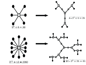
Figure 1: Example of the dendro operation on single-check codes. Numbers count beliefs (degrees of freedom) required for LP evaluation.

However, many of the constraints associated with the check beliefs are not really required for decoding. It was argued in [7] that the number of useful constraints per check can be reduced to $\sim q_{\alpha}$. This result was improved in [14], where an impressive $O(1)$, thus $q_{\alpha}$-independent, scaling in the number of required constraints was experimentally achieved by adaptive scheduling of constraints and early termination in the case of successful decoding. (Note that the number of log-likelihood dependent scheduling operations required here is $\sim q_{\alpha}$, thus complexity of the entire algorithm is linear in $q_{\alpha}$.) Armed with the observations of [7, 14] and also of [15], where a BP-style relaxation of LP achieving overall linear scaling in $q_{\alpha}$ was proposed, we extend the list of useful tricks by the dendro scheme explained below. The scheme, demonstrating overall linear scaling in $q_{\alpha}$, does not require log-likelihood dependent adaptation.

Our strategy in dealing with the checks of high degree is through modification of the graphical model (Tanner graph) of the code. We simply replace the check by a dendro, i.e. tree, graph with the same number of leaves as the number of bit neighbors, $q_{\alpha}$, in the original graph. All bits inside the dendro construction, i.e. these that are not leaves, are the auxiliary, punctured, bits. The new dendro-checks are all of degree three, while the punctured bits are all of degree two. The punctuated bits are not transmitted, thus the log-likelihoods at the bits are zeros. The construction is illustrated in Fig. 1.

The simple dendro construction is advantageous for decoding as the total number of beliefs is seriously reduced. It becomes linear in $q_{\alpha}$ at $q_{\alpha}\to\infty$ for the dendro-code correspondent to a single-check code, as opposed to $2^{q_{\alpha}}$ for the original code.

It is straightforward to verify that the codewords of the original code and of the dendro-code are in one-to-one correspondence. Indeed, the codewords of a code are controlled by checks, formally expressed in terms of the product of the Kronecker symbols in Eq. (1). On the other hand, any check constraint can be explicitly rewritten as

$$\delta\biggl{(}\prod_{i\in\alpha}(-1)^{\sigma_{i}},1\biggr{)}=\sum_{{\bm{\sigma}}^{(pun)}_{\alpha}}\prod_{\beta\in d(\alpha)}\delta\biggl{(}\prod_{j\in\beta}(-1)^{\sigma_{j}},1\biggr{)}$$

$$\times\prod_{\beta\in\partial(\alpha)}\delta\biggl{(}\prod_{j\in\beta}(-1)^{\sigma_{j}},\prod_{i\in\beta}(-1)^{\sigma_{i}}\biggr{)},$$ (4)

where $d(\alpha)$[$\partial(\alpha)$] are the sets of dendro checks replacing check $\alpha$ such that the checks neighbor only [not only] punctured bits; and ${\bm{\sigma}}^{(pun)}_{\alpha}$ is the vector of punctured bits originating from the check, $\alpha$, of the original code. The lhs and rhs of Eq. (4) correspond to the check constraints of the original code and the dendro code respectively. Putting it in a less formal way, once the values of the bits of the original codes are known, the punctured bits of the respective dendro code are unambiguously restored. Furthermore, since the punctuated bits are not transmitted and have zero log-likelihoods, one finds that MAP decoding of the original code and of its dendro counterpart generate exactly the same results.

Comparing the LP decoding of the two codes, it is useful to turn to the notion of the graph covers discussed in [9, 10, 11]. The pseudo-codewords of an LDPC code are in one-to-one correspondence with the codewords of the respective family of graph-cover LDPC codes. The graph covers are constructed by replicating the total number of checks and nodes of the code by the same positive integer, the cover degree, and by connecting the bits/checks with replicas of their original neighbors. The family of graph covers can be generated both for the original code and for the respective dendro code. The number of graph covers of the same degree is larger for the dendro-code then for its original code. More specifically, for each standard-cover one gets a family of equivalent dendro-covers. Each dendro-cover from the family will get exactly the same set of codewords as of the original code. This statement follows directly from the previous paragraph. Therefore, the set of pseudo-codewords, understood as the codewords of the set of covers, will be exactly the same for the original code and its dendro-counterpart. Let us notice that this statement does not necessarily mean that decoding of the same output configuration by the two codes will necessarily give the same result.

IV Error-floor and Pseudo-codeword-search algorithm [12]

If the LP decoding does not decode to a correct codeword then it usually yields a non-codeword pseudo-codeword, which is a special configuration of beliefs containing some rational values [7, 10]. An important characteristic of the decoding performance is the Frame Error Rate (FER) calculating the probability of a decoding failure. FER decreases as SNR increases. The form of this dependence gives an ultimate description of the coding performance. Any decoding to a non-codeword pseudo-codeword is a failure. Decoding to a codeword can also be a failure, which counts as a failure under the ML decoding. For large SNR, splitting of the two (FER vs SNR) curves, representing ML decoding and approximate decoding (say LP decoding) is due to the pseudo-codewords. The actual asymptotics of the two curves for the AWGN channel at the largest SNRs, in the so-called error-floor domain, are $\mbox{FER}_{\mbox{\scriptsize ML}}\sim\exp(-d_{\mbox{\scriptsize ML}}\cdot s^{2}/2)$ and $\mbox{FER}_{\mbox{\scriptsize LP}}\sim\exp(-d_{\mbox{\scriptsize LP}}\cdot s^{2}/2)$, where $d_{\mbox{\scriptsize ML}}$ is the Hamming distance of the code and the $d_{\mbox{\scriptsize LP}}$ is the effective distance of the code, specific for the LP decoding. The LP asymptotic is normally shallower than the one of MAP, $d_{\mbox{\scriptsize LP}}<d_{\mbox{\scriptsize ML}}$. The error floor can start or change its behavior at values of FER inaccessible by Monte-Carlo simulations. This fact emphasizes the importance of the pseudo-codewords analysis [19].

For a generic binary linear code that is used for data communication over binary-input output-symmetric channel, it is easy to show that FER is invariant under change of the original codeword (sent into the channel). Therefore, for the purpose of FER evaluation, it is sufficient to analyze statistics exclusively for the case of one known original codeword, and the choice of zero codeword is natural. Then, calculating the effective distance of a code, one makes an assumption that there exists a special configuration (or a few special configurations) of the noise, instantons according to the terminology of [17], describing the large SNR error-floor asymptotic for FER. Suppose a pseudo codeword, $\tilde{\bm{\sigma}}=\{\tilde{\sigma_{i}}=b_{i}(1);\ i=1,\dots,N\}$, corresponding to the most damaging configuration of the noise (instanton), ${\bm{x}}_{\mbox{\scriptsize inst}}$, is found. Then finding the instanton configuration itself (i.e. respective configuration of the noise) is not a problem, one only needs to maximize the transition probability with respect to the noise field, ${\bm{x}}$, taken at ${\bm{\sigma}}=0$ under the condition that the self-energy calculated for the pseudo-codeword in the given noise field ${\bm{x}}$ is zero (i.e. equal to the value of the self energy for the zero code word). The resulting expression for the optimal configuration of the noise (instanton) in the case of the AWGN channel is ${\bm{x}}_{\mbox{\scriptsize inst}}=(\tilde{\bm{\sigma}}\sum_{i}\tilde{\sigma}_{i})/(2\sum_{i}\tilde{\sigma}_{i}^{2})$, and the respective effective distance is $d_{\mbox{\scriptsize LP}}=(\sum_{i}\tilde{\sigma}_{i})^{2}/\sum_{i}\tilde{\sigma}_{i}^{2}$. This definition of the effective distance was first described in [20], with the first applications of this formula to LP decoding discussed in [9] and [11]. Note also that the expressions are reminiscent of the formulas derived by Wiberg and co-authors in [21] and [18], in the context of the computational tree analysis applied to iterative decoding with a finite number of iterations.

Let us now describe the pseudo-codeword-search algorithm, introduced in [12]. Start: Initiate a starting configuration of the noise, ${\bm{x}}^{(0)}$. Noise is counted from the zero codeword and it should be sufficiently large to guarantee convergence of LP to a pseudo-codeword different from the zero codeword. Step 1: The LP decodes ${\bm{\sigma}}^{(k)}$ to $\{b_{i}^{(\mbox{\scriptsize LP},k)}(\sigma_{i}),b_{\alpha}^{(\mbox{\scriptsize LP},k)}(\sigma_{\alpha})\}$. Step 2: Find ${\bm{y}}^{(k)}$, the weighted median in the noise space between the pseudo codeword, ${\bm{\sigma}}^{(k)}$, and the zero codeword. The AWGN expression for the weighted median is ${\bm{y}}^{(k)}=({\bm{\sigma}}^{(k)}\sum_{i}\sigma_{i}^{(k)})/(2\sum_{i}\big{(}\sigma_{i}^{(k)}\big{)}^{2})$. Step 3: If ${\bm{y}}^{(k)}={\bm{y}}^{(k-1)}$, then $k_{*}=k$ and the algorithm terminates. Otherwise go to Step 2, assigning ${\bm{x}}^{(k+1)}={\bm{y}}^{(k)}+\varepsilon$ for some very small $\varepsilon$. ($+\varepsilon$ prevents decoding into the zero codeword, keeping the result of decoding within the erroneous domain.) Output configuration ${\bm{y}}^{(k_{*})}$ is the configuration of the noise that belongs to the error-surface surrounding the zero codeword. (The error-surface separates the domain of correct LP decisions from the domain of incorrect LP decisions.) Moreover, locally, i.e. for the given part of the error-surface equidistant from the zero codeword and the pseudo codeword ${\bm{\sigma}}^{(k_{*})}$, ${\bm{y}}^{(k_{*})}$ is the nearest point of the error-surface to the zero codeword.

We repeat the algorithm many times, picking the initial noise configuration randomly, however guaranteeing that it would be sufficiently far from the zero codeword so that the result of the LP decoding (first step of the algorithm) is a pseudo-codeword distinct from the zero codeword. We showed in [12] that the algorithm converges, and that it does so in a relatively small number of iterations. The error-floor performance of the coding scheme is characterized by the spectra of the effective distances derived over multiple evaluations of the pseudo-codeword-search algorithm.

We can easily extend the pseudo-codeword-search algorithm to the dendro-LDPC codes decoded by LP. The dendro version of the algorithm is actually identical to the one described above with the exception of how the punctured nodes are treated. First, one should always zero the log-likelihoods at all the punctured nodes and, second, calculating the weighted medians, one should exclude punctured nodes from the sum.

V Pseudo-codeword spectra: Results and Analysis

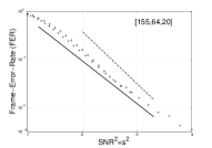
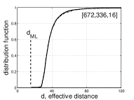
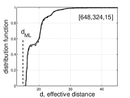
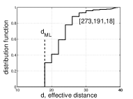
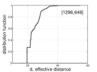
Figure 2: The two plots from the first row show results of Monte-Carlo simulations for the $[155,64,20]$ and $[672,336,16]$ codes. Stars and diamonds stand for BP (1024 iterations) and LP decodings respectively. Straight and dashed lines mark the asymptotic controlled by the pseudo-codewords with the lowest effective weight and the MAP asymptotic respectively. The six remaining plots from the three lower rows show probability density function of the effective distance (that we also refer to as frequency spectra) for the six codes analyzed. Solid and dashed curves (almost coinciding, thus difficult to distinguish) correspond to the dendro-codes and the original codes respectively. We indicate position of the respective Hamming distance by a marker, whenever it is known.

We experimented with the $[155,64,20]$ code [22], Margulis $p=7$ code $[672,336,16]$ [23]; $[648,324,15]$, $[648,432,12]$ and $[1296,648]$ codes from the 802.11n draft [5], and the $[273,191,18]$ projective geometry code. The results are shown in Fig. (2). Dendro counterparts were generated for all the codes. For the dendro-codes, and whenever feasible for the original codes, we have found the frequency spectra of the pseudo-codewords by the method explained in Section IV. We experimentally confirmed the prediction of Section III, that the set of pseudo-codewords of the original codes and respective dendro-codes are identical. Moreover, we found that the corresponding pseudo-codeword spectra are almost indistinguishable (up to variation in the number of samples) from each other. For the first two codes from the list, we also performed direct Monte-Carlo simulations.

The rest of the manuscript contains discussion of the results. Comparing $[155,64,20]$ and $[672,336,16]$ codes we conclude that the two codes demonstrate qualitatively different features, that are consistently seen both in the MC simulations and the pseudo-codewords frequency spectra.

In the case of the $[155,64,20]$ code, the pseudo-codeword spectrum starts form $d_{min}\approx 16.404$ and grows continuously to the higher values, e.g. passing though $d_{ML}=20$ without any visible anomaly. The growth, starting immediately from $d_{min}$, is fast, indicating that the frequency of the low-effective distance configurations is considerable, i.e. $O(1)$. This form of the pseudo-codeword spectra is consistent with what is seen in the MC simulations: the error-floor asymptotic of FER, $\sim\exp(-d_{min}s^{2}/2)$, corresponding to the pseudo-codeword with the lowest effective weight, sets in early.

The behavior demonstrated by the $[672,336,16]$ code is different. Looking, first, at the pseudo-codeword spectra, we find that the configuration with the lowest effective distance is actually a codeword with $d_{ML}=16$. We also find in the spectrum two other codewords corresponding to $d=24$ and $d=25$. Even though the low distance codewords were observed, their frequencies were orders of magnitude smaller then of other pseudo-codeword configurations found at $d\gtrsim 27.33$. Emergence of the gap suggests that in spite of the fact that the relatively small Hamming distance describes the largest SNR asymptotic of FER, the moderate SNR asymptotic is actually controlled by the continuous part of the pseudo-codeword spectra above the gap. This prediction is indeed consistent with MC results shown in the second plot from the top row of Fig. (2), see also [25], where the intermediate asymptotic, $\sim\exp(-27.33s^{2}/2)$, set in at moderate SNRs, changes to a shallower curve with the SNR increase.

The two-stage scenario, when the lowest distance configuration is the one of a codeword separated by a gap from the rest of the spectrum, is also seen in the frequency spectra of the $[648,324,15]$ and $[648,432,12]$ codes, shown in the third row of the Fig. (2). However the gaps in the later cases are much smaller than in the $[672,336,16]$ case. The behavior of the $[273,191,18]$ code can also be attributed to the same type, with the exception of one really special feature of the code. Here one gets a whole stairway of low distance codewords observed with significant frequencies. Note that the original projective geometry code has highly connected checks, with degree $17$, thus the aforementioned analysis is feasible only for the dendro version of the code.

Analyzing the $[1296,648]$ code, one finds that, on the one hand, the configuration with the lowest effective distance, $d_{min}\approx 19.6$, is a non-codeword pseudo-codeword, like in the case of the $[155,64,20]$ code. On the other hand, this lowest configuration is separated by a noticeable gap from the next one with $d\approx 21.75$, like in the case of the $[672,336,16]$ code. However, the lowest weight configuration is not rare, thus suggesting that the FER vs SNR dependence for this code will likely show a one stage error-floor associated with the lowest effective distance.

This work was carried out under the auspices of the National Nuclear Security Administration of the U.S. Department of Energy at Los Alamos National Laboratory under Contract No. DE-AC52-06NA25396.

References

- [1] R.G. Gallager, Low density parity check codes (MIT PressCambride, MA, 1963).
- [2] C. Berrou, A. Glavieux, P. Thitimajshima, Near Shannon Limit error-correcting coding and decoding: Turbo codes, Proceedings IEEE International Conference on Communications, 23-26 May 1993, Geneva, Switzerland; p.1064-70 vol.2
- [3] D.J.C. MacKay, Good error-correcting codes based on very sparse matrices, IEEE Trans. Inf. Theory 45 (2) 399-431 (1999).
- [4] C. E. Shannon, “A mathematical theory of communication,” Bell Syst. Tech. J., vol. 27, pt. I, pp. 379-423, 1948; pt. II, pp. 623-656, 1948.
- [5] IEEE P802.11n/D1.05 October 2006, Wireless LAN Medium Access Control (MAC) and Physical Layer (PHY) specifications - Enhancements for Higher Throughput (Draft).
- [6] E. M. Kurtas and B. Vasic (editors), Advanced Error Control Techniques for Data Storage Systems, New York: CRC Press, 2005.
- [7] J. Feldman, M. Wainwright, D.R. Karger, Using linear programming to decode binary linear codes, IEEE IT51, 954 (2005).
- [8] J.S. Yedidia, W.T. Freeman, Y. Weiss, Constructing Free Energy Approximations and Generalized Belief Propagation Algorithms, IEEE IT51, 2282 (2005).
- [9] R. Koetter, P.O. Vontobel, Graph covers and iterative decoding of finite-length codes, Proc. 3rd International Symposium on Turbo Codes & Related Topics, Brest, France, p. 75–82, Sept. 1–5, 2003.
- [10] P.O. Vontobel, and R. Koetter, On the relationship between LP decoding and Min-Sum Algorithms Decoding, ISITA 2004, Parma Italy.
- [11] P.O. Vontobel, R. Koetter, Graph-cover decoding and finite-length analysis of message-passing iterative decoding of LDPC codes, arXiv:cs.IT/0512078.
- [12] M. Chertkov, M. Stepanov, An Efficient Pseudo-Codeword-Search Algorithm for Linear Programming Decoding of LDPC Codes, arXiv:cs.IT/0601113, submitted to IEEE Transactions on Information Theory.
- [13] M. Chertkov, V. Chernyak, Loop Calculus Helps to Improve Belief Propagation and Linear Programming Decodings of Low-Density-Parity-Check Codes, invited talk at 44th Allerton Conference (September 27-29, 2006, Allerton,IL), arXiv:cs.IT/0609154.
- [14] M.H. Taghavi N., P.H. Siegel, Adaptive Linear Programming Decoding, Proceedings of the IEEE ISIT, Seattle 2006, arxiv:cs.IT/0601099.
- [15] P.O. Vontobel and R. Koetter, Towards Low-Complexity Linear-Programming Decoding, Proc. 4th Int. Symposium on Turbo Codes and Related Topics, Munich, Germany, April 3-7, 2006, arxiv:cs/0602088.
- [16] M. Yannakakis, Expressing combinatorial optimization problems by linear programs, J. of Computer and System Sciences, 43(3) 441-466 (1991).
- [17] M.G. Stepanov, V. Chernyak, M. Chertkov, B. Vasic, Diagnosis of weakness in error correction codes: a physics approach to error floor analysis, Phys. Rev. Lett. 95, 228701 (2005) [See also http://www.arxiv.org/cond-mat/0506037 for extended version with Supplements.]
- [18] N. Wiberg Codes and decoding on general graphs, Ph.D. thesis, Linköping University, 1996.
- [19] T. Richardson, Error floors of LDPC codes, 2003 Allerton conference Proccedings.
- [20] G.D. Forney, Jr., R. Koetter, F.R. Kschischang, and A. Reznik, On the effective weights of pseudocodewords for codes defined on graphs with cycles, in Codes, Systems, and Graphical Models (Minneapolis, MN, 1999)(B. Marcus and J. Rosenthal, eds.) vol. 123 of IMA Vol. Math. Appl.., pp. 101-112 Springer Verlag, New York, Inc., 2001.
- [21] N. Wiberg, H-A. Loeliger, R. Kotter, Codes and iterative decoding on general graphs, Europ. Transaction Telecommunications 6, 513 (1995).
- [22] R.M. Tanner, D. Sridhara, T. Fuja, A class of group-structured LDPC codes, Proc. of ISCTA 2001, Ambleside, England.
- [23] G.A. Margulis, Explicit construction of graphs without short circles and low-density codes, Combinatorica 2, 71 (1982).
- [24] D.J.C. MacKay and M.S. Postol, Weaknesses of Margulis and Ramanujan-Margulis Low-Density Parity-Check codes, Proceedings of MFCSIT2002, Galway, http://www.inference.phy.cam.ac.uk/mackay/ abstracts/margulis.html .
- [25] M.G. Stepanov, M. Chertkov, Instanton analysis of Low-Density-Parity-Check codes in the error-floor regime, arXiv:cs.IT/0601070, Proceeding of ISIT 2006, July 2006 Seattle.