Asynchronous Distributed Searchlight Scheduling

Abstract

This paper develops and compares two simple asynchronous distributed searchlight scheduling algorithms for multiple robotic agents in nonconvex polygonal environments. A searchlight is a ray emitted by a agent which cannot penetrate the boundary of the environment. A point is detected by a searchlight if and only if the point is on the ray at some instant. Targets are points which can move continuously with unbounded speed. The objective of the proposed algorithms is for the agents to coordinate the slewing (rotation about a point) of their searchlights in a distributed manner, i.e., using only local sensing and limited communication, such that any target will necessarily be detected in finite time. The first algorithm we develop, called the DOWSS (Distributed One Way Sweep Strategy), is a distributed version of a known algorithm described originally in 1990 by Sugihara et al [9], but it can be very slow in clearing the entire environment because only one searchlight may slew at a time. In an effort to reduce the time to clear the environment, we develop a second algorithm, called the PTSS (Parallel Tree Sweep Strategy), in which searchlights sweep in parallel if guards are placed according to an environment partition belonging to a class we call PTSS partitions. Finally, we discuss how DOWSS and PTSS could be combined with with deployment, or extended to environments with holes.

1 Introduction

Consider a group of robotic agents acting as guards in a nonconvex polygonal environment, e.g., a floor plan. For simplicity, we model the agents as point masses. Each agent is equipped with a single unidirectional sweeping sensor called a searchlight (imagine a ray of light such as a laser range finder emanating from each agent). A searchlight aims only in one direction at a time and cannot penetrate the boundary of the environment, but its direction can be changed continuously by the agent. A point is detected by a searchlight at some instant iff the point lies on the ray. A target is any point which can move continuously with unbounded speed. The Searchlight Scheduling Problem is to

Find a schedule to slew a set of stationary searchlights such that any target in an environment will necessarily be detected in finite time.

A searchlight problem instance consists of an environment and a set of stationary guard positions. Obviously there can only exist a search schedule if all points in the environment are visible by some guard. For a graphical description of our objective, see Fig. 1 and 2.

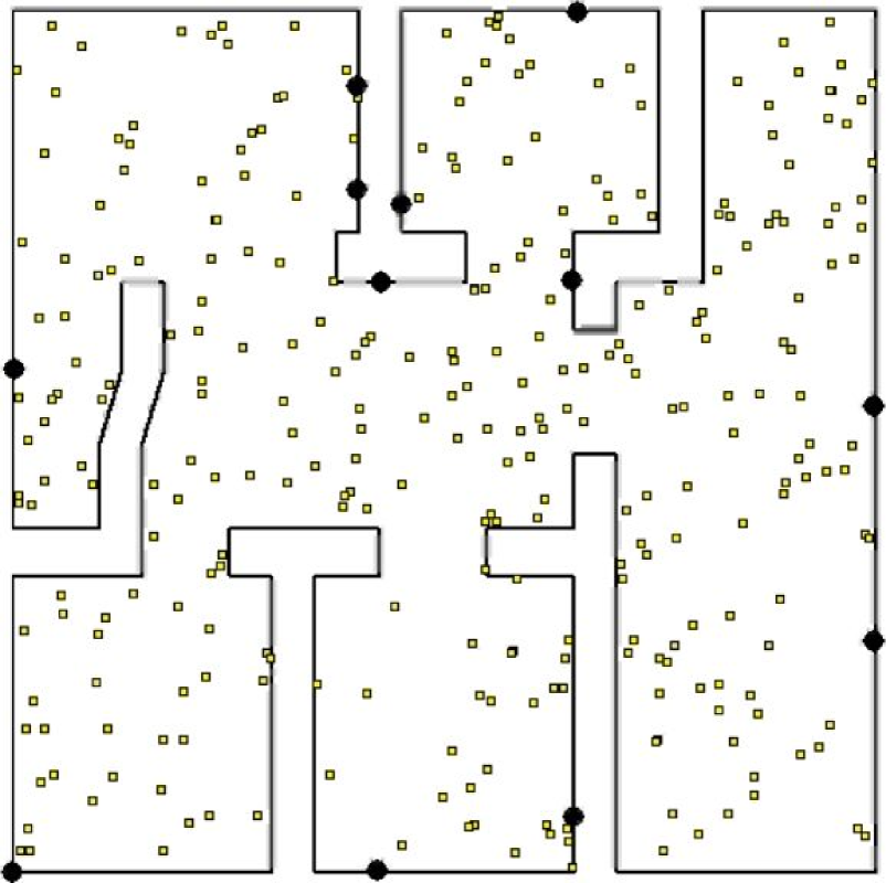
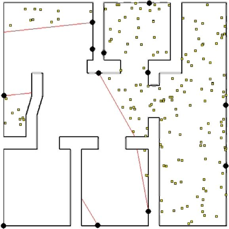
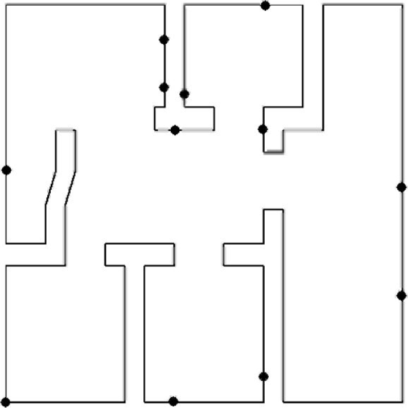
Fig. 1: Simulation results of the PTSS algorithm described in Section 4.2, executed by agents (black dots) in a polygon shaped like a typical floor plan. Left to right , moving targets (small yellow squares) disappear as they are detected by searchlights (red). The cleared region grows until it encompasses the entire environment.

To our knowledge the searchlight scheduling problem was first introduced in the inspiring paper by Sugihara, Suzuki and Yamashita in [9], which considers simple polygonal environments and stationary searchlights. [11] extends [9] to consider guards with multiple searchlights (they call a guard possessing $k$ searchlights a $k$-searcher) and polygonal environments containing holes. Some papers involving mobile searchlights, sometimes calling them flashlights or beam detectors, are [4], [12], [8], and [5]. Closely related is the Classical Art Gallery Problem, namely that of finding a minimum set of guards s.t. the entire polygon is visible. There are many variations on the art gallery problem which are wonderfully surveyed in [10], [6], and [7].

Assume now that each member of the group of guards is equipped with omnidirectional line-of-sight sensors. By a line-of-sight sensor, we mean any device or combination of devices that can be used to determine, in its line-of-sight, (i) the position or state of another guard, and (ii) the distance to the boundary of the environment. By omnidirectional, we mean that the field-of-vision for the sensor is $2\pi$ radians. There exist distributed algorithms to deploy asynchronous mobile robots with such omnidirectional sensors into nonconvex environments, and they are guaranteed to converge to fixed positions from which the entire environment is visible, e.g., [2] and [3]. At least one algorithm exists which guarantees the ancillary benefit of the final guard positions having a connected visibility graph ([3]).

Once a set of guards seeing the entire environment has been established, it may be desired to continuously sweep the environment with searchlights so that any target will be detected in finite time. The main contribution of this paper is the development of two different asynchronous distributed algorithms to solve the searchlight scheduling problem. Correctness and bounds on time to clear nonconvex polygonal environments are discussed. The first algorithm we develop, called the DOWSS (Distributed One Way Sweep Strategy, Sec. 4.1, is a distributed version of a known algorithm described originally in [9], but it can be very slow in clearing the entire environment because only one searchlight may slew at a time. On-line processing time required by agents during execution of DOWSS is relatively low, so that the expedience with which an environment can be cleared is essentially limited by the maximum angular speed searchlights may be slewn at. In an effort to reduce the time to clear the environment, we develop a second algorithm, called the PTSS (Parallel Tree Sweep Strategy, Sec. 4.2), which sweeps searchlights in parallel if guards are placed according to an environment partition belonging to a class we call PTSS partitions. That we analyze the time it takes to clear an environment, given a bound on the angular slewing velocity, is a unique feature among all papers involving searchlights to date. Finally, we discuss how DOWSS and PTSS can be extended for environments with holes and for mobile guards performing a coordinated search. Until now, there has been no description in the literature of a scalable distributed algorithm for clearing an environment with mobile searchlights (1-searchers), though [4] and [12], for example, offer some centralized approaches.

We begin with some technical definitions, statement of assumptions, and brief description of the known centralized algorithm called the one way sweep strategy (appears, e.g., in [9], [11], [12]). We then develop a partially asynchronous model, a distributed one way sweep strategy, and our new algorithm the parallel tree sweep strategy.

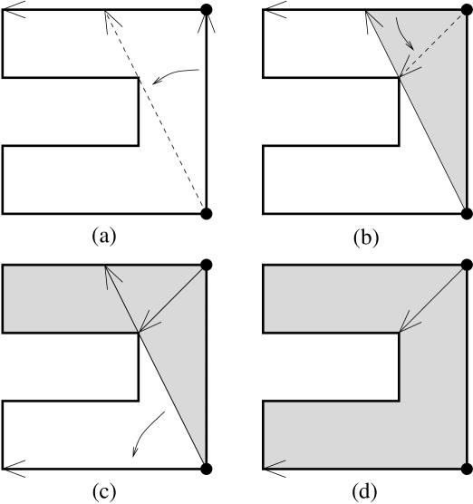
Fig. 2: A simple example of a searchlight schedule. From (a) to (d): First the lower agent aims at the upper agent and sweeps until it hits a visibility gap. Next, the upper agent sweeps the other side of the visibility gap so the lower agent can continue sweeping the remainder of the environment. No target, no matter how fast, would be able to avoid being detected by this slewing sequence.

2 Preliminaries

2.1 Notation

We begin by introducing some basic notation. We let ${\mathbb{R}}$, ${\mathbb{S}}^{1}$, and ${\mathbb{N}}$ refer to the set of real numbers, the circle, and natural numbers, respectively. Given two points $x,y\in{\mathbb{R}}^{2}$, we let $[x,y]$ signify the closed segment between $x$ and $y$. Similarly, $]x,y[$ is the open segment between $x$ and $y$, $[x,y[$ represents the set $]x,y[\operatorname{\cup}\{x\}$ and $]x,y]$ is the set $]x,y[\operatorname{\cup}\{y\}$. Given a finite set $X$, let $|X|$ represent the cardinality of the set. Also, we shall use $P$ to refer to tuples of elements in ${\mathbb{R}}^{2}$ of the form $(p^{[0]},\dots,p^{[N-1]})$ (these will be the locations of the agents), where $N$ denotes the total number of agents.

We now turn our attention to the environment we are interested in and to the concepts of visibility in such environments. Let $\mathcal{E}$ be a simple polygonal environment, possibly nonconvex. By simple, we mean that $\mathcal{E}$ does not contain any hole and the boundary does not intersect itself. Throughout this paper, $n$ will refer to the number of edges of $\mathcal{E}$ and $r$ the number of reflex vertices. A point $q\in\mathcal{E}$ is visible from $p\in\mathcal{E}$ if $[p,q]\subset\mathcal{E}$. The visibility set $\mathcal{V}(p)\subset\mathcal{E}$ from a point $p\in\mathcal{E}$ is the set of points in $\mathcal{E}$ visible from $p$. A visibility gap of a point $p$ with respect to some region $R\subset\mathcal{E}$ is defined as any line segment $[a,b]$ such that $]a,b[\subset\operatorname{int}(R)$, $[a,b]\subset\partial\mathcal{V}(p)$, and it is maximal in the sense that $a,b\in\partial R$ (intuitively, visibility gaps block off portions of $R$ not visible from $p$). The visibility graph $\mathcal{G}_{\rm vis}$ of a set of agents $P$ in environment $\mathcal{E}$ is the undirected graph with $P$ as the set of vertices and an edge between two agents iff they are visible to each other.

We now introduce some notation specific to the searchlight problem. An instance of the searchlight problem is specified by a pair $(\mathcal{E},P)$, where $\mathcal{E}$ is an environment and $P$ is a set of searchlight locations in $\mathcal{E}$. For convenience, we will refer to the $i$th searchlight as $s^{[i]}$ (which is located at $p^{[i]}\in{\mathbb{R}}^{2}$), and $S=\{s^{[0]},\dots,s^{[N-1]}\}$ will be the set of all searchlights. $\theta^{[i]}$ will denote the configuration angle of the searchlight in radians from the positive horizontal axis, and $\Theta=\{\theta^{[0]},\dots,\theta^{[N-1]}\}$ the joint configuration. So, if we say, e.g., aim $s^{[i]}$ at point $e$, what we really mean is set $\theta^{[i]}$ equal to an angle such that the $i$th searchlight is aimed at $e$. Note that searchlights do not block visibility of other searchlights.

The next few definitions were taken from [9].

Definition 1 (schedule).

The schedule of a searchlight $s^{[i]}\in S$ is a continuous function $\theta^{[i]}:[0,t^{*}]\mapsto{\mathbb{S}}^{1}$, where $[0,t^{*}]$ is an interval of real time.

The ray of $s^{[i]}$ at time $t\in[0,t^{*}]$ is the intersection of $\mathcal{V}(p^{[i]})$ and the semi-infinite ray starting at $p^{[i]}$ with direction $\theta^{[i]}(t)$. $s^{[i]}$ is said to be aimed at a point $x\in\mathcal{E}$ in some time instant if $x$ is on the ray of $s^{[i]}$. A point $x$ is illuminated if there exists a searchlight aimed at $x$.

Definition 2 (separability).

Two points in $\mathcal{E}$ are separable at time $t\in[0,t^{*}]$ if every curve connecting them in the interior of $\mathcal{E}$ contains an illuminated point, otherwise they are nonseparable.

Definition 3 (contamination and clarity).

A point $x\in\mathcal{E}$ is contaminated at time zero if and only if it is not illuminated. The point $x$ is contaminated at time $t\in]0,t^{*}]$ iff $\exists y\in\mathcal{E}$ such that (1) $y$ is contaminated at some $t^{\prime}\in[0,t[$, (2) $y$ is not illuminated at any time in the interval $[t^{\prime},t]$, and (3) $x$ and $y$ are nonseparable at $t$. A point which is not contaminated is called clear. A region is said to be contaminated if it contains a contaminated point, otherwise it is clear.

Definition 4 (search schedule).

Given $\mathcal{E}$ and a set of searchlight locations $P=\{p^{[0]},\ldots,p^{[N-1]}\}$, the set $\Theta=\{\theta^{[0]},\ldots,\theta^{[N-1]}\}$ is a search schedule for $(\mathcal{E},P)$ if $\mathcal{E}$ is clear at $t^{*}$.

2.2 Problem description and assumptions

We now describe the problem we solve and the assumptions made. The Distributed Searchlight Scheduling Problem is to

Design a distributed algorithm for a network of autonomous robotic agents in fixed positions, who will coordinate the slewing of their searchlights so that any target in an environment will necessarily be detected in finite time. Furthermore, these agents are to operate using only information from local sensing and limited communication.

What is precisely meant by local sensing and limited communication will become clear in later sections. The following standing assumptions will be made about every searchlight instance in this paper:

1. The environment is a simple polygon with finitely many reflex vertices.
   Comments: Compactness is a practical assumption for sensor range limitations. Simple connectedness means no holes. Having only finitely many reflex vertices precludes problems such as arise from fractal environments and will be important for proving the algorithms terminate in finite time.

2. Every point in the environment is visible from some agent and there are a finite number $N\in{\mathbb{N}}$ of agents.
   Comments: If there were some point in the environment not visible by any agent, then a target could remain there undetected for infinite time.

3. For every connected component of $\mathcal{G}_{\rm vis}$, there is at least one agent located on the boundary of the environment.
   Comments: This will be important for proving the algorithms terminate without failure. It also implies every agent is either on the boundary of the environment or visible from some other agent. If there existed an agent $i$ located at a point $p_{i}$ in the interior of the environment and not visible by any other agent, then there would exist $\epsilon>0$ such that $\overline{B}_{\epsilon}(p_{i})\cap\mathcal{V}(p_{j})=\emptyset$ for $i\neq j$. A target could thus evade detection by remaining in $\overline{B}_{\epsilon}(p_{i})$ and simply staying on the opposite side of agent $i$ as $l_{i}$ points.

2.3 One Way Sweep Strategy (OWSS)

This section describes informally the centralized recursive One Way Sweep Strategy (OWSS hereinafter) originally introduced in [9]. The reader is referred to [9] for a detailed description. Centralized OWSS also appears in [12] and [11]. OWSS is a method for clearing a subregion of a simple 2D region $\mathcal{E}$ determined by the rays of searchlights. The subregions of interest are the so-called semiconvex subregions of $\mathcal{E}$ supported by a set of searchlights at a given time and are defined as follows:

Definition 5 (semiconvex subregion).

$\mathcal{E}$ is always a semiconvex subregion of $\mathcal{E}$ supported by $\emptyset$. Furthermore, any $R\subset\mathcal{E}$ is a semiconvex subregion of $\mathcal{E}$ supported by a set of searchlights $S_{\rm sup}$ if both of the following hold:

1. It is enclosed by a segment of $\partial\mathcal{E}$ and the rays of some of the searchlights in $S_{\rm sup}$.

2. The interior of $R$ is not visible from any searchlight in $S_{\rm sup}$.

The term “semiconvex” comes from the fact that any reflex vertex of a semiconvex subregion is also a reflex vertex of $\mathcal{E}$. In polygonal environments, all semiconvex subregions are polygons. The schedule used in Fig. 2 was based on OWSS, but as a more general example, consider Fig. 3. To clear the environment $\mathcal{E}$, which is a semiconvex subregion supported by $\emptyset$, we may begin by selecting an arbitrary searchlight on the boundary, say $s^{[0]}$. The first searchlight selected to clear an environment will be called the root. $s^{[0]}$ aims as far clockwise (cw hereinafter) as possible so that it is aligned along the cw-most edge. $l_{i}$ will then slew couterclockwise (ccw hereinafter) through the environment, stopping incrementally whenever it encounters a visibility gap. The only visibility gap $s^{[0]}$ encounters produces the semiconvex subregion $R$ (thick border). At this time, another searchlight which sees across the visibility gap and is not in the interior of $R$, in this case $s^{[1]}$, is chosen to begin sweeping the area in $R$ not seen by $s^{[0]}$. Notice we have marked angles $\phi_{\rm start}$ and $\phi_{\rm finish}$. These are the cw-most and ccw-most directions, resp., in which $s^{[1]}$ can aim at some point in $R$. $s^{[1]}$ will slew from $\phi_{\rm start}$ to $\phi_{\rm finish}$ and in the process encounter visibility gaps, each producing the semiconvex subregions $R_{1}$, $R_{j}$, and $R_{m}$, which must be cleared by $s^{[2]}$ and/or $s^{[3]}$. As soon as $R$ is clear (when $\theta^{[1]}=\phi_{\rm finish}$), $s^{[0]}$ can continue slewing until it is pointing along the wall immediately to its left at which time the entire environment is clear. The recursive nature of OWSS should be apparent at this point. Note that in OWSS (and DOWSS described later) it is actually arbitrary whether a searchlight slews cw or ccw over a semiconvex subregion, but to simplify the discussion we always use ccw.

Fig. 3: One Way Sweep Strategy (OWSS) clears, by slewing $s^{[1]}$, the semiconvex subregion $R$ (thick border) supported by $s^{[0]}$. $\ s^{[1]}$ must stop incrementally at each of its visibility gaps $[a_{1},b_{1}]$, $[a_{j},b_{j}]$, and $[a_{m},b_{m}]$. In this recursive process, the regions ($R_{1}$, $R_{j}$, $R_{m}$) behind the visibility gaps become semiconvex subregions supported by $\{s^{[0]},s^{[1]}\}$, and must be cleared using only the remaining searchlights ($s^{[2]}$ and $s^{[3]}$) .

3 Asynchronous Network of Agents with Searchlights

In this section we lay down the sensing and communication framework for the searchlight equipped agents which will be able to execute the proposed algorithms. Each agent is able to sense the relative position of any point in its visibility set as well as identify visibility gaps on the boundary of its visibility set. The agents’ communication graph $\mathcal{G}_{\rm comm}$ is assumed to connected. An agent can slew its searchlight continuously in any direction and turn it on or off.

Each of the $N$ agents has a unique identifier (UID), say $i$, and a portion of memory dedicated to outgoing messages with contents denoted by $\mathcal{M}^{[i]}$. Agent $i$ can broadcast its UID together with $\mathcal{M}^{[i]}$ to all agents within its communication region, where the communication region is defined differently in each algorithm. Such a broadcast will be denoted by $\textup{BROADCAST}(i,\mathcal{M}^{[i]})$. We assume a bounded time delay, $\delta>0$, between a broadcast and the corresponding reception.

Each agent repeatedly performs the following sequence of actions between any two wake-up instants, say instants $T^{[i]}_{l}$ and $T^{[i]}_{l+1}$ for agent $i$:

1. SPEAK, that is, send a BROADCAST repeatedly at $\delta$ intervals, until it starts slewing;

2. LISTEN for a time interval at least $\delta$;

3. PROCESS and LISTEN after receiving a valid message;

4. SLEW to an angle decided during PROCESS.

See Figure 4 for a schematic illustration of the above schedule.

Fig. 4: Sequence of actions performed by an agent $i$ in between two wake-up instants. Note that a $\textup{BROADCAST}(i,\mathcal{M}^{[i]})$ is an instantaneous event taking place where there is a vertical pulse, where as the PROCESS, LISTEN and SLEW actions take place over an interval. The SLEW interval may be empty if the agent does not sweep.

Any agent $i$ performing the SLEW action does so according to the following discrete-time control system (cf Section 2.3):

$$\theta^{[i]}(t+\Delta t)=\theta^{[i]}(t)+u^{[i]},$$ (1)

where the control is bounded in magnitude by $s_{\rm max}$. The control action depends on time, values of variables stored in local memory, and the information obtained from communication and sensing. The subsequent wake-up instant $T_{l+1}^{[i]}$ is the time when the agent stops performing SLEW and is not predetermined. This network model is identical to that used for distributed deployment in [2] and [3], and is similar in spirit to the partially asynchronous model described in [1].

4 Distributed Algorithms

In this section we design distributed algorithms for a network of agents as described in Section 3, where no agent has global knowledge of the environment or locations of all other agents.

4.1 Distributed One Way Sweep Strategy (DOWSS)

Once one understands OWSS as in Section 2.3, esp. its recursive nature, performing one way sweep of an environment in a distributed fashion is fairly straightforward. We give here an informal description and supply a pseudocode in Tab. 1 (A more detailed pseudocode, which we refer to in the proofs, can be found in the appendix, Tab. 3). In our discussion root/parent/child will refer to the relative location of agents in the simulated one way sweep recursion tree. In this tree, each node corresponds to a one way slewing action by some agent. A single agent may correspond to more than one node, but only one node at a time . To begin DOWSS, some agent (the root), say $i$, can aim as far cw as possible and then begin slewing until it encounters a visibility gap. Paused at a visibility gap, agent $i$ broadcasts a call for help to the network. For convenience, call the semiconvex subregion which $i$ needs help clearing $R$. All agents not busy in the set of supporting searchlights $S_{\rm sup}$ (indeed at the zeroth level of recursion only the root is in $S_{\rm sup}$), who also know they can see a portion of $\operatorname{int}(R)$ but are not in $\operatorname{int}(R)$, volunteer themselves to help $i$. Agent $i$ then chooses a child and the process continues recursively. In DOWSS as in Tab. 1, an agent needing help always chooses the first child to volunteer, but some other criteria could be used, e.g., who sees the largest portion of $R$. Whenever a child is finished helping, i.e., clearing a semiconvex subregion, it reports to its parent so the parent knows they may continue slewing.

The only subtle part of DOWSS is getting agents to recognize, without global knowledge of the environment, that they see the interior of a particular semiconvex subregion which some potential parent needs help clearing. More precisely, suppose some agent $l$ must decide whether to respond as a volunteer to agent $i$’s help request to clear a semiconvex subregion $R$. Agent $l$ must calculate if it actually satisfies the criterion in Tab. 3, line 3 of PROCESS, namely $p^{[l]}\notin\operatorname{int}(R)$ and $\operatorname{int}(R)\cap\mathcal{V}(p^{[l]})\neq\emptyset$. This is accomplished by agent $i$ sending along with its help request an oriented polyline $\psi$ (see Tab. 3, line 3 of SPEAK). By an oriented polyline we mean that $\psi$ consists of a set of points listed according to some orientation convention, e.g., so that if one were to walk along the points in the order listed, then the interior of $R$ would always be to the right. The polyline encodes the portion of $\partial R$ which is not part of $\partial\mathcal{E}$ and the orientation encodes which side of $\psi$ is the interior of $R$. Notice that for this to work, all agents must have a common reference frame. Whenever the root broadcasts a polyline, it is just a line segment, but as recursion becomes deeper, an agent needing help may have to calculate a polyline consisting of a portion of its own beam and its parent’s polyline. The polyline may even close on itself and create a convex polygon. Examples of these scenarios are illustrated by in Fig 5. We conclude our description of DOWSS with the following theorem.

Theorem 6 (Correctness of DOWSS).

Given a simple polygonal environment $\mathcal{E}$ and agent positions $P=(p^{[0]},\ldots,p^{[N-1]})$, let the following conditions hold:

1. the standing assumptions are satisfied;

2. all agents $i\in\{0,\ldots,N-1\}$ have a common reference frame;

3. $p^{[0]}\in\partial\mathcal{E}$;

4. the agents operate under DOWSS.

Then $\mathcal{E}$ is cleared in finite time.

Proof.

As in Theorem 2 of [9], whenever an agent, say $i$, needs help clearing a semiconvex subregion $R$, there is some available agent $l$ satisfying $p{[l]}\notin\operatorname{int}(R)$ and $\operatorname{int}(R)\cap\mathcal{V}(p^{[l]})\neq\emptyset$. This comes from the standing assumption that for every connected component of $\mathcal{G}_{\rm vis}$, there is at least one agent on the environment boundary. Now since visibility sets are closed, we may demand additionally that agent $l$ sees a portion of the oriented polyline $\psi$ sent to it by $i$. This means that in an execution of DOWSS, some $l$ will always be able to recognize, using only knowledge of $\mathcal{V}(p^{[l]})$ and $\psi$ from local sensing and limited communication, that it is able to help. We conclude DOWSS simulates OWSS. ∎

Fig. 5: An example execution of DOWSS. The configuration in (a) results from $s^{[0]}$ clearing the very top of the region with help of $s^{[2]}$, $s^{[3]}$, and $s^{[4]}$ followed by $s^{[1]}$ attempting to clear the semiconvex subregion below where $s^{[0]}$ is aimed. When $s^{[1]}$ gets stuck, it requests help by broadcasting the thick black polyline in (a), in this case just a line segment. $s^{[2]}$ then helps $s^{[1]}$ but gets stuck right off, so it broadcasts the thick black polyline shown in (b). Next $s^{[3]}$ helps $s^{[2]}$ but gets stuck and broadcast the polyline in (c). Similarly $s^{[4]}$ broadcasts the polyline in (d), in this case a convex polygon, which only $s^{[5]}$ can clear. In general, information passed between agents during any execution of DOWSS will be in the form of either an oriented line segment (a), a general oriented polyline (b and c), or a convex polygon (d).

We now give an upper bound on the time it takes DOWSS to clear the environment assuming the searchlights slew at some constant angular velocity $\omega$, and that communication and processing time are negligible.

Lemma 7 (DOWSS Time to Clear Environment).

Let agents in a network executing DOWSS slew their searchlights with angular speed $\omega$. Then the time required to clear an environment with $r$ reflex vertices is no greater than $\frac{2\pi}{\omega}\frac{1-r^{N}}{1-r}$.

Proof.

There are only finitely many ($r$) reflex vertices of $\mathcal{E}$, and finitely many guards ($N$). Recall each visibility gap encountered during an execution of DOWSS produces a semiconvex subregion whose reflex vertices necessarily are part of $\partial\mathcal{E}$. This means the number of visibility gaps encountered by any agent when sweeping from $\phi_{\rm start}$ to $\phi_{\rm finish}$ (at any level of the recursion tree) can be no greater than $r$, i.e., refering to line 8 of PROCESS in Tab. 3, $|G|=m\leq r$. Since the number of agents available to sweep a semiconvex subregion decreases by one for each level of recursion, the maximum depth of the recursion tree is upper bounded by $N-1$. It is apparent the number of nodes in the recursion tree cannot exceed $1+r+r^{2}+\dots+r^{N-1}=\frac{1-r^{N}}{1-r}$. ∎

It is not known whether this bound is tight, but at least examples as in Fig. 6 can be constructed where DOWSS and OWSS run in $\mathcal{O}(r^{2})$ ($\Rightarrow\mathcal{O}(n^{2})$) time if guards are chosen malevolently. A key point is that DOWSS and OWSS do not specify (i) how to place guards given an environment, or (ii) how to optimally choose guards at each step given a set of guards. These are interesting unsolved problems in their own right which we do not explore in this paper.

Fig. 6: An example from a class of searchlight instances for which malevolent guard choice in OWSS or DOWSS implies time to clear the environment is $\mathcal{O}(r^{2})$ (and therefore $\mathcal{O}(n^{2})$). Here $r=4$ reflex vertices are oriented on the bottom so that $s^{[r]}=s^{[4]}$ in the upper right corner sees the entire environment. $r-1=3$ guards are placed in the upper left and $s^{[0]}$ is chosen as the root. $s^{[0]}$ clears up to the first reflex vertex (grey) where it stops and calls upon $s^{[1]}$ for help. $s^{[1]}$ then calls upon $s^{[2]}$ which likewise calls upon $s^{[3]}$. This happens every time $s^{[0]}$ stops (dashed lines) at the other $r-1$ reflex vertices. The recursion tree of such an execution has $1+r(r-1)$ nodes, thus the environment is cleared in $\mathcal{O}(r^{2})$ time.

Another performance measure of a distributed algorithm is the size of the messages which must be communicated.

Lemma 8 (DOWSS Message Size).

If the environment has $n$ sides, $r$ reflex vertices, and $N$ agents then the polyline (passed as a message between agents during DOWSS) consists of a list of no more than $\min\{r+1,N\}$ points in ${\mathbb{R}}^{2}$. Furthermore, since $r\leq n-3$, the list consists of no more than $n-2$ points in ${\mathbb{R}}^{2}$.

Proof.

For every segment (which is a segment of some searchlight’s beam) in such a polyline, there corresponds a unique reflex vertex of the environment. The correspondence comes from the fact that at a given time every searchlight supporting a semiconvex subregion has its searchlight aimed at a reflex vertex where it’s visibility is occluded. The uniqueness comes from the fact that if two searchlights support the same semiconvex subregion, say $R$, and are aimed at the same reflex vertex, then only one of the searchlights’ beams can actually constitute a portion of $\partial R$ of positive length. This shows the polyline can consist of no more than $r$ segments and therefore $r+1$ vertices. Also, in the worst case, the polyline grows by one edge for each level of recursion. Such polylines start out as a line segment (defined by two points) and the recursion depth cannot exceed $N-1$. We conclude the maximum number of points defining any polyline is $\min\{r+1,N\}$. ∎

Table 1: Asynchronous Schedule for Distributed One Way Sweep Strategy (cf Fig. 3, 4, 5, Tab. 3)

Name: DOWSS Goal: Agents in the network coordinate their searchlight slewing to clear an environment $\mathcal{E}$. Assumes: Agents are stationary and have a completely connected communication topology with no packet loss. Sweeping is initialized by a root.


For time $t>0$, each agent executes the following actions between any two wake up instants according to the schedule in Section 3:

SPEAK   Broadcast either    (i) a request for help, (ii) a message to engage a child, or (iii) a signal of task completion to a parent. LISTEN   Listen for either    (i) a help request from a potential parent, (ii) volunteers to help, (iii) engagement by parent, or (iv) current child reporting completion. PROCESS    (i) Use oriented polyline from potential parent with information from sensing to check if able to help, or (ii) if engaged, compute wayangles, visibility gaps and oriented polylines. SLEW    (i) Aim at start angle and switch searchlight on, (ii) slew to next angle, or (iii) slew to finish angle and switch searchlight off.

That DOWSS allows flexibility in guard positions (only standing assumptions required) may be an advantage if agents are immobile. However, DOWSS only allowing one searchlight slewn at a time is a clear disadvantage when time to clear the environment is to be minimized. This lead us to design the algorithm in the next section.

4.2 Positioning Guards for Parallel Sweeping

The DOWSS algorithm in the previous section is a distributed message-passing and local sensing scheme to perform searchlight scheduling given a priori the location of the searchlights. Given an arbitrary positioning, time to completion of DOWSS can be large; see Lemma 7 and Figure 6.

The algorithm we design in this section, called the Parallel Tree Sweep Strategy (PTSS), provides a way of choosing searchlight locations and a corresponding schedule to achieve faster clearing times. PTSS works roughly like this: According to some technical criteria described below, the environment is partitioned into regions called cells with one agent located in each cell. Additionally, the network possesses a distributed representation of a rooted tree. By distributed representation we mean that every agent knows who its parent and children are. Using the tree, agents slew their searchlights in a way that expands the clear region from the root out to the leaves, thus clearing the entire environment. Since agents may operate in parallel, time to clear the environment is linear in the height of the tree and thus $\mathcal{O}(n)$. Guaranteed linear time to completion is a clear advantage over DOWSS which can be quadratic or worse (see Lemma 7 and Fig. 6). Before describing PTSS more precisely, we need a few definitions.

Definition 9.

1. A set $\mathcal{S}\subset{\mathbb{R}}^{2}$ is star-shaped if there exists a point $p\in\mathcal{S}$ with the property that all points in $\mathcal{S}$ are visible from $p$. The set of all such points of a given star-shaped set $\mathcal{S}$ is called the kernel of $\mathcal{S}$ and is denoted by $\ker(\mathcal{S})$.

2. Given a compact subset $\mathcal{E}$ of ${\mathbb{R}}^{2}$, a partition of $\mathcal{E}$ is is a collection of sets $\{\mathcal{P}^{[0]},\ldots,\mathcal{P}^{[N-1]}\}$ such that $\operatorname{\cup}_{i=0}^{N-1}\mathcal{P}^{[i]}=\mathcal{E}$ where $\mathcal{P}^{[i]}$’s are compact, simply connected subsets of $\mathcal{E}$ with disjoint interiors. $\{\mathcal{P}^{[0]},\ldots,\mathcal{P}^{[N-1]}\}$ will be called cells of the partition.

For our purposes a gap (which visibility gap is a special case of) will refer to any segment $[q,q^{\prime}]$ with $q,q^{\prime}\in\partial\mathcal{E}$ and ${]q,q^{\prime}[}\in\mathring{\mathcal{E}}$. The cells of the partitions we consider will be separated by gaps.

Definition 10 (PTSS partition).

Given a simple polygonal environment $\mathcal{E}$, a partition $\{\mathcal{P}^{[0]},\ldots,\mathcal{P}^{[N-1]}\}$ is a PTSS partition if the following conditions are true:

1. $\mathcal{P}^{[i]}$ is a star-shaped cell for all $i\in\{0,\ldots,N-1\}$;

2. the dual graph of the partition is a tree;

3. a root, say $\mathcal{P}^{[0]}$, of the dual graph may be chosen so that $\ker(\mathcal{P}^{[0]})\cap\partial\mathcal{E}\neq\emptyset$, and for any node other than the root, say $\mathcal{P}^{[k]}$ with parent $\mathcal{P}^{[j]}$, we have that $(\mathcal{P}^{[j]}\cap\mathcal{P}^{[k]})\cap\ker(\mathcal{P}^{[k]})\cap\partial\mathcal{E}\neq\emptyset$.

Definition 11.

Given a PTSS partition $\{\mathcal{P}^{[0]},\ldots,\mathcal{P}^{[N-1]}\}$ of $\mathcal{E}$ and a root cell $\mathcal{P}^{[0]}$ of the partition’s dual graph satisfying the properties discussed in Definition 10, the corresponding (rooted) PTSS tree is defined as follows:

1. the node set $(p^{[0]},\ldots,p^{[N-1]})$ is such that $p^{[0]}\in\ker(\mathcal{P}^{[0]})\cap\partial\mathcal{E}$ and for $k>1$, $p^{[k]}\in(\mathcal{P}^{[j]}\cap\mathcal{P}^{[k]})\cap\ker(\mathcal{P}^{[k]})\cap\partial\mathcal{E}$, where $\mathcal{P}^{[j]}$ is the parent of $\mathcal{P}^{[k]}$ in the dual graph of the partition;

2. there exists an edge $(p^{[j]},p^{[k]})$ if and only if there exists an edge $(\mathcal{P}^{[j]},\mathcal{P}^{[k]})$ in the dual graph.

We now describe two examples of PTSS partitions seen in Fig. 7. The left configuration in Fig. 7 results from what we call a Reflex Vertex Straddling (RVS hereinafter) deployment. RVS deployment begins with all agents located at the root followed by one agent moving to the furthest end of each of the root’s visibility gaps, thus becoming children of the root. Likewise, further agents are deployed from each child to take positions on the furthest end of the children’s visibility gaps located across the gaps dividing the parent from the children. In this way, the root’s cell in the PTSS partition is just its visibility set, but the cells of all successive agents consist of the portion of the agents’ visibility sets lying across the gaps dividing their cells from their respective parents’ cells. It is easy to see that in final positions resulting from an RVS deployment, agents see the entire environment.

Lemma 12.

RVS deployment requires, in general, no more than $r+1\leq n-2$ agents to see the entire environment from their final positions. In an orthogonal environment, no more than $\frac{n}{2}-2$ agents are required.

Proof.

Follows from the fact that in addition to the root, no more than one agent will be placed for each reflex vertex (only reflex vertices occlude visibility). ∎

See Fig. 1 for simulation results of PTSS executed by agents in an RVS configuration. The right configuration in Fig. 7 results from the deployment described in [3] in which an orthogonal environment is partitioned into convex quadrilaterals.

Lemma 13.

The deployment described in [3] requires no more than $\frac{n}{2}-2$ agents to see the entire (orthogonal) environment from their final positions.

Proof.

See [3]. ∎

Both of the PTSS configurations in these examples may be generated via distributed deployment algorithms in which agents perform a depth-first, breadth-first, or randomized search on the PTSS tree constructed on-line. Please refer to [2] and [3] for a detailed description of these algorithms.

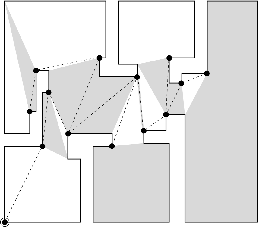
Fig. 7: Left are agent positions resulting from a Reflex Vertex Straddling (RVS) deployment. Right are agent positions resulting from the deployment described in [3] in which an orthogonal environment is partitioned into convex quadrilaterals. The PTSS partitions are shown by coloring the cells alternating grey and white (caution: grey does not depict clarity here). Dotted lines show edges of the PTSS tree where the circled agent is the root.

We now turn our attention to the pseudocode in Tab. 2 (A more detailed pseudocode, which we refer to in the proofs, can be found in the appendix, Tab. 4) and describe PTSS more precisely. Suppose some agents are positioned in an environment according to a PTSS partition and tree with agent $1$ as the root. PTSS begins by agent $1$ pointing its searchlight along a wall in the direction $\phi_{\rm start}$ and then slewing away from the wall toward $\phi_{\rm finish}$, pausing whenever it encounters the first side of a gap, say $\phi_{j}$, where $j$ is odd. Paused at $\phi_{j}$, agent $1$ sends a message to its child at that gap, say agent $2$, so that agent $2$ knows it should aim its searchlight across the gap. Once agent $2$ has its searchlight safely aimed across the gap, it sends a message to agent $1$ so that agent $1$ knows it may continue slewing over the whole gap. When agent $1$ has reached the other side of the gap at $\phi_{j+1}$, agent $1$ sends a message to agent $2$ and both agents continue clearing the rest of their cells concurrently, stopping at gaps and coordinating with children as necessary. In this way, the clear region expands from the root to the leaves at which time the entire environment has been cleared. We arrive at the following lemmas and correctness result.

Lemma 14 (Expanding a Clear Region Across a Gap).

Suppose an environment is endowed with a PTSS partition and tree, and that agent $i$ is a parent of agent $j$ (see Fig. 8). Then a clear region may always be expanded across the gap from $\mathcal{P}^{[i]}$ to $\mathcal{P}^{[j]}$ by $s^{[j]}$ first aiming across the gap and waiting for $s^{[i]}$ to slew over the gap. Both agents may then continue clearing the remainder of their respective cells concurrently.

Proof.

This obviously hold for the scenario in Fig. 8. Using the definition of PTSS partition, it is clear any general PTSS parent-child relationship is reducible to the case in Fig. 8. ∎

Fig. 8: Expanding a clear region (grey) across a gap (thick dashed segment [v, v’]) from cell $\mathcal{P}^{[i]}$ to cell $\mathcal{P}^{[j]}$ may always be accomplished by the child ($s^{[j]}$) aiming across the gap and waiting for the parent ($s^{[i]}$) to slew over the gap. Both agents may then continue clearing the remainder of their respective cells.

Theorem 15 (Correctness of PTSS).

Given a simple polygonal environment $\mathcal{E}$ and agent positions $P=(p^{[0]},\ldots,p^{[N-1]})$, let the following conditions hold:

1. the standing assumptions are satisfied;

2. all agents $i\in\{0,\ldots,N-1\}$ are positioned in a PTSS partition and rooted tree with agent $1$ as the root;

3. the agents operate under PTSS.

Then $\mathcal{E}$ is cleared in finite time.

Proof.

Follows immediately from Lemma 14. ∎

Since multiple branches of the PTSS tree may be cleared concurrently, and using Lemmas 12 and 13, we have the next lemma (assuming processing and communication time are negligible, cf. Lemma 7).

Lemma 16 (PTSS Time to Clear Environment).

Let the agents in a network executing PTSS slew their searchlights with angular speed $\omega$. Then time required to clear an environment is

1. linear in the height of the PTSS tree;

2. no greater than $\frac{2\pi}{\omega}(r+1)\leq\frac{2\pi}{\omega}(n-2)$ if agents are in final positions according to an RVS deployment;

3. no greater than $\frac{\pi}{\omega}(n-2)$ if agents are in final positions in an orthogonal polygon according to an RVS deployment or the deployment described in [3].

Proof.

With communication time neglibile, each child will wait for it’s parent a maximum time of $\frac{2\pi}{\omega}$. It now suffices to observe that the maximum length of any parent-child sequence is just the height of the PTSS tree. ∎

Looking at the SPEAK section of Tab. 4, it is easy to see that message size is constant (cf. Lemma 8).

Lemma 17 (PTSS Message Size).

Messages passed between agents executing PTSS have constant size.

Table 2: Asynchronous Schedule for Parallel Tree Sweep Strategy (cf Fig. 4, 8, 7, Tab. 4)

Name: PTSS Goal: Agents in the network coordinate their searchlight slewing to clear an environment $\mathcal{E}$. Assumes: Agents are statically positioned as nodes in a PTSS partition and tree, and each knows a priori the gaps of its cell and UIDs of the corresponding children and parent. Sweeping is initialized by the root.


For time $t>0$, each agent executes the following actions between any two wake up instants according to the schedule in Section 3:

SPEAK   Broadcast either (i) a command for a child to aim across a gap, (ii) a confirmation to a parent when aimed across gap, or (iii) when finished slewing over a gap, a signal of completion to the child. LISTEN   Listen for either (i) instruction from a parent to aim across a gap, (ii) confirmation from a child aimed across a gap, or (iii) confirmation that parent has passed the gap. PROCESS   When first engaged, compute wayangles where coordination with children will be necessary. SLEW    (i) Aim at start angle and switch searchlight on, (ii) slew to next wayangle, or (iii) slew to finish angle and switch searchlight off.

Requiring guards to be situated in a PTSS tree may be more restrictive than the mere standing assumptions required by DOWSS, but the time savings using PTSS over DOWSS can be considerable. Though we have given two examples of how to construct a PTSS tree, it is not clear how to construct one which clears an environment in minimum time among all possible PTSS trees. It is also not clear how to optimally choose the root of the tree (point of deployment). However, if information about an environment layout is known a priori and one may choose the root location, then an exhaustive strategy may be adopted whereby all possible root choices are compared.

5 Conclusions

In this paper we have provided two solutions to the distributed searchlight scheduling problem. DOWSS requires guards satisfying the standing assumptions, has message size $\mathcal{O}(n)$, and sometimes takes time $\mathcal{O}(r^{2})$ to clear an environment. PTSS requires agents are positioned according to a PTSS tree, has constant message size, and takes time linear in the height of the PTSS tree to clear the environment. We have given two procedures for constructing PTSS trees, one requiring no more than $r\leq n-3$ guards for a general polygonal environment, and two requiring no more than $\frac{n-2}{2}$ guards for an orthogonal environment. Guards slew through a total angle no greater than $2\pi$, so the upper bounds on the time for PTSS to clear an environment with these partitions are $\frac{2\pi}{\omega}r\leq\frac{2\pi}{\omega}(n-3)$ and $\frac{\pi}{\omega}(n-2)$, respectively. Because PTSS allows searchlights to slew concurrently, it generally clears an environment much faster than DOWSS. However, the comparison is not completely fair since DOWSS does not specify how to choose guards but PTSS does.

To extend DOWSS and PTSS for environments with holes, one simple solution is to add one guard per hole, where a simply connected environment is simulated by the extra guards using their beams to connect the holes to the outer boundary. Another straightforward extension for PTSS would be to combine it directly with a distributed deployment algorithm such as those in [2] and [3], so that deployment and searchlight slewing happen concurrently. This suggests an interesting problem we hope to explore in the future, namely minimizing the time to perform a coordinated search given a limited number of mobile guards. Other considerations for the future include loosening the requirements in the definition of the PTSS partition, and incorporating in our model sensor constraints such as limited depth of field and beam incidence.

6 Appendix: Extended versions of Tab. 1 and 2 referred to in proofs

Table 3: Asynchronous Schedule for Distributed One Way Sweep Strategy (cf Fig. 3, 4, 5, Tab. 1)

Name: DOWSS Goal: Agents in the network coordinate their searchlight slewing to clear an environment $Q$. Assumes: Agents are stationary and have a completely connected communication topology with no packet loss. Sweeping is initialized by a root who’s uid is 1.
The root initially has ${\rm state}=4$ and all other agents begin with ${\rm state}=1$, where possible states are $1,2,3,\ldots,12$. Aditionally, each agent $i\in\{0,\ldots,N-1\}$, possesses local variables ${\rm parent}$, ${\rm child}$, $\psi_{\rm parent}$, $\psi_{\rm temp}$, $j$, $G$, $\Phi$, $\phi_{\rm start}$, $\phi_{\rm finish}$, $\Psi$, and $u$, all initially empty. As needed to clarify ownership, a superscript with square brackets indicates the UID of the agent to whom a variable belongs. For time $t>0$, each agent $i$ executes the following between any two wake up instants according to the schedule in Section 3: SPEAK 1: while ${\rm state}=7$ or ${\rm state}=8$ do 2:    {request help} 3:    $\textup{BROADCAST}(i,\psi_{j}(t),{\tt help})$ 4:    ${\rm state}\leftarrow 8$ 5: while ${\rm state}=2$ do 6:    {volunteer to help} 7:    $\textup{BROADCAST}(i,{\rm parent}(t),\psi_{\rm temp}(t),{\tt volunteer})$ 8:    ${\rm state}\leftarrow 3$ 9: while ${\rm state}=9$ do 10:    {engage a child} 11:    $\textup{BROADCAST}(i,{\rm child}(t),\psi_{j}(t),{\tt selected})$ 12:    ${\rm state}\leftarrow 10$ 13: while ${\rm state}=12$ do 14:    {report to parent when complete} 15:    $\textup{BROADCAST}(i,{\rm parent},\psi_{\rm parent}(t),{\tt complete})$ 16:    ${\rm state}\leftarrow 1$ LISTEN 1: while ${\rm state}=1$ or ${\rm state}=3$ do 2:    {listen for help request} 3:    if $\textup{RECEIVE}(i^{\prime},\psi^{[i^{\prime}]}_{j^{\prime}}(t-\tau),{\tt help})$, where $0\leq\tau\leq\delta$ then 4:       $\psi_{\rm temp}\leftarrow\psi^{[i^{\prime}]}_{j^{\prime}}(t-\tau)$; ${\rm state}\leftarrow 3$ 5: while ${\rm state}=8$ do 6:    {listen for volunteers} 7:    if $\textup{RECEIVE}(i^{\prime},{\rm parent}^{[i^{\prime}]}(t-\tau),\psi^{[i^{\prime}]}_{\rm temp}(t-\tau),{\tt volunteer})$, where $0\leq\tau\leq\delta$, ${\rm parent}^{[i^{\prime}]}(t-\tau)=i$, and $\psi^{[i^{\prime}]}_{\rm temp}(t-\tau)=\psi_{j}$ then 8:       ${\rm child}\leftarrow i^{\prime};{\rm state}\leftarrow 9$ 9: while ${\rm state}=3$ do 10:    {listen for engagement by parent} 11:    if $\textup{RECEIVE}(i^{\prime},{\rm child}^{[i^{\prime}]},\psi^{[i^{\prime}]}_{j^{\prime}}(t-\tau),{\tt selected})$, where $0\leq\tau\leq\delta$, where ${\rm child}^{i^{\prime}}=i$ then 12:       ${\rm parent}\leftarrow i^{\prime};\psi_{\rm parent}\leftarrow\psi^{[i^{\prime}]}_{j^{\prime}}(t-\tau);{\rm state}\leftarrow 4$ 13:    else if $\textup{RECEIVE}(i^{\prime},{\rm child}^{[i^{\prime}]},\psi^{[i^{\prime}]}_{j^{\prime}}(t-\tau),{\tt selected})$, where $0\leq\tau\leq\delta$, where ${\rm child}^{[i^{\prime}]}\neq i$ then 14:       ${\rm state}\leftarrow 1$ 15: while ${\rm state}=10$ do 16:    {listen for child to report completion} 17:    if  $\textup{RECEIVE}(i^{\prime},{\rm parent}^{[i^{\prime}]},\psi^{[i^{\prime}]}_{\rm parent}(t-\tau),{\tt complete})$, where $0\leq\tau\leq\delta$  then 18:       if $j<m$ then 19:          $j\leftarrow j+1;{\rm state}\leftarrow 6$ 20:       else if $j=m$ then 21:          ${\rm state}\leftarrow 11$ PROCESS 1: while ${\rm state}=3$ do 2:    {use $\psi_{\rm temp}$ and $\mathcal{V}(p^{[i]})$ to check if able to help} 3:    if able to see across oriented polyline $\psi_{\rm temp}$ into semiconvex subregion and not located in interior of that subregion then 4:       ${\rm state}\leftarrow 2$ 5: while ${\rm state}=4$ do 6:    {when first engaged, perform geometric computations; note visibility gaps are listed ccw and radially outwards} 7:    Compute $\phi_{\rm start}$ and $\phi_{\rm finish}$ {start and finish angles} 8:    Compute $G\leftarrow(g_{1},\ldots,g_{m})$ {visibility gaps} 9:    Compute $\Phi\leftarrow(\phi_{1},\ldots,\phi_{m})$ {resp. angles of visibility gaps} 10:    Compute $\Psi\leftarrow(\psi_{1},\ldots,\psi_{m})$ {polyline for each visibility gap} 11:    $j\leftarrow 1$ {initialize slewing counter} 12:    ${\rm state}\leftarrow 5$ SLEW 1: while ${\rm state}=5$ do 2:    {aim at start angle and switch searchlight on} 3:    $\theta^{[i]}\leftarrow\phi_{\rm start}$ 4:    ${\rm state}\leftarrow 6$ 5: while ${\rm state}=6$ do 6:    {slew to next angle} 7:    while $\theta^{[i]}<\phi_{j}$ do 8:       $u\leftarrow\frac{\min\{s_{\rm max},||\phi_{j}-\theta^{[i]}||\}}{||\phi_{j}-\theta^{[i]}||}(\phi_{j}-\theta^{[i]})$ 9:       $\theta^{[i]}\leftarrow\theta^{[i]}+u$ 10:    ${\rm state}\leftarrow 7$ 11: while ${\rm state}=11$ do 12:    {slew to finish angle and switch searchlight off} 13:    while $\theta^{[i]}<\phi_{\rm finish}$ do 14:       $u\leftarrow\frac{\min\{s_{\rm max},||\phi_{\rm finish}-\theta^{[i]}||\}}{||\phi_{\rm finish}-\theta^{[i]}||}(\phi_{\rm finish}-\theta^{[i]})$ 15:       $\theta^{[i]}\leftarrow\theta^{[i]}+u$ 16:    ${\rm state}\leftarrow 12$

Table 4: Asynchronous Schedule for Parallel Tree Sweep Strategy (cf Fig. 4, 8, 7, Tab. 2)

Name: PTSS Goal: Agents in the network coordinate their searchlight slewing to clear an environment $Q$. Assumes: Agents are statically positioned as nodes in a PTSS partition and tree, and each knows a priori the gaps of its cell and UIDs of the corresponding children and parent. Sweeping is initialized by a root who’s UID is 1. Agents need only communicate with their parents and children.
The root initially has ${\rm state}=2$ and all other agents begin with ${\rm state}=1$, where possible states are $1,2,\ldots,10$. Additionally each agent $i\in\{0,\ldots,N-1\}$, possesses local variables ${\rm parent}$, $\Phi$, $\phi_{\rm start}$, $\phi_{\rm finish}$, $C$, $j$, and $u$, all initially empty. As needed to clarify ownership, a superscript with square brackets indicates the UID of the agent to whom a variable belongs. For time $t>0$, each agent $i$ executes the following between any two wake up instants according to the schedule in Section 3: SPEAK 1: while ${\rm state}=7$ do 2:    {tell child to aim across gap} 3:    $\textup{BROADCAST}({\rm child}_{j},{\tt aim\_across\_gap})$ 4:    ${\rm state}\leftarrow 8$ 5: while ${\rm state}=4$ do 6:    {tell parent when aimed across gap} 7:    $\textup{BROADCAST}(i,{\tt aimed\_across\_gap})$ 8:    ${\rm state}\leftarrow 5$ 9: while ${\rm state}=9$ do 10:    {tell child when finished slewing over gap} 11:    $\textup{BROADCAST}({\rm child}_{j},{\tt gap\_passed})$ 12:    if $j<m$ then 13:       $j\leftarrow j+1;{\rm state}\leftarrow 6$ 14:    else if $j=m$ then 15:       ${\rm state}\leftarrow 10$ LISTEN 1: while ${\rm state}=1$ do 2:    {listen for instruction from parent to aim across gap} 3:    if $\textup{RECEIVE}({\rm child}^{[i^{\prime}]},{\tt aim\_across\_gap})$ and $i={\rm child}^{[i^{\prime}]}$ then 4:       ${\rm state}\leftarrow 2$ 5: while ${\rm state}=8$ do 6:    {listen for confirmation from child aimed across gap} 7:    if $\textup{RECEIVE}(i^{\prime},{\tt aimed\_across\_gap})$ and $i^{\prime}={\rm child}_{j}$ then 8:       $j\leftarrow j+1;{\rm state}\leftarrow 6$ 9: while ${\rm state}=5$ do 10:    {listen for confirmation that parent has passed the gap} 11:    if $\textup{RECEIVE}({\rm child}^{[i^{\prime}]},{\tt gap\_passed})$ and $i={\rm child}^{[i^{\prime}]}$ then 12:       ${\rm state}\leftarrow 6$ PROCESS 1: while ${\rm state}=2$ do 2:    {when first engaged, perform geometric computations} 3:    Compute $\phi_{\rm start}$ and $\phi_{\rm finish}$ {start and finish angles} 4:    Compute $\Phi\leftarrow(\phi_{1},\ldots,\phi_{m})$ {ordered gap endpoint angles} 5:    Compute $C\leftarrow({\rm child}_{1},\ldots,{\rm child}_{m})$ {resp. child UIDs} 6:    $j\leftarrow 1$; {initialize slewing counter} 7:    ${\rm state}\leftarrow 3$ SLEW 1: while ${\rm state}=3$ do 2:    {aim at start angle and switch searchlight on} 3:    $\theta^{[i]}\leftarrow\phi_{\rm start}$ 4:    ${\rm state}\leftarrow 4$ 5: while ${\rm state}=6$ do 6:    {slew to next angle} 7:    while $\theta^{[i]}<\phi_{j}$ do 8:       $u\leftarrow\frac{\min\{s_{\rm max},||\phi_{j}-\theta^{[i]}||\}}{||\phi_{j}-\theta^{[i]}||}(\phi_{j}-\theta^{[i]})$ 9:       $\theta^{[i]}\leftarrow\theta^{[i]}+u$ 10:    if $j$ is odd then 11:       ${\rm state}\leftarrow 7$ 12:    else if $j$ is even then 13:       ${\rm state}\leftarrow 9$ 14: while ${\rm state}=10$ do 15:    {slew to finish angle and switch searchlight off} 16:    while $\theta^{[i]}<\phi_{\rm finish}$ do 17:       $u\leftarrow\frac{\min\{s_{\rm max},||\phi_{\rm finish}-\theta^{[i]}||\}}{||\phi_{\rm finish}-\theta^{[i]}||}(\phi_{\rm finish}-\theta^{[i]})$ 18:       $\theta^{[i]}\leftarrow\theta^{[i]}+u$ 19:    ${\rm state}\leftarrow 1$

References

- [1] D. P. Bertsekas and J. N. Tsitsiklis, Parallel and Distributed Computation: Numerical Methods, Athena Scientific, Belmont, MA, 1997.
- [2] A. Ganguli, J. Cortés, and F. Bullo, Distributed deployment of asynchronous guards in art galleries, in American Control Conference, Minneapolis, MN, June 2006, pp. 1416–1421.
- [3] , Visibility-based multi-agent deployment in orthogonal environments, in American Control Conference, New York, July 2007. To appear.
- [4] B. P. Gerkey, S. Thrun, and G. Gordon, Visibility-based pursuit-evasion with limited field of view, International Journal of Robotics Research, 25 (2006), pp. 299–315.
- [5] J. H. Lee, S. M. Park, and K. Y. Chwa, Simple algorithms for searching a polygon with flashlights, Information Processing Letters, 81 (2002), pp. 265–270.
- [6] J. O’Rourke, Art Gallery Theorems and Algorithms, Oxford University Press, Oxford, UK, 1987.
- [7] T. C. Shermer, Recent results in art galleries, IEEE Proceedings, 80 (1992), pp. 1384–1399.
- [8] B. Simov, G. Slutzki, and S. M. LaValle, Pursuit-evasion using beam detection, in IEEE Int. Conf. on Robotics and Automation, 2000.
- [9] K. Sugihara, I. Suzuki, and M. Yamashita, The searchlight scheduling problem, SIAM Journal on Computing, 19 (1990), pp. 1024–1040.
- [10] J. Urrutia, Art gallery and illumination problems, in Handbook of Computational Geometry, J. R. Sack and J. Urrutia, eds., North-Holland, Amsterdam, the Netherlands, 2000, pp. 973–1027.
- [11] M. Yamashita, I. Suzuki, and T. Kameda, Searching a polygonal region by a group of stationary k-searchers, Information Processing Letters, 92 (2004), pp. 1–8.
- [12] M. Yamashita, H. Umemoto, I. Suzuki, and T. Kameda, Searching for mobile intruders in a polygonal region by a group of mobile searchers, Algorithmica, 31 (2001), pp. 208–236.