Open-architecture Implementation of
Fragment Molecular Orbital Method
for Peta-scale Computing

Abstract

We present our perspective and goals on high-performance computing for nanoscience in accordance with the global trend toward “peta-scale computing.” After reviewing our results obtained through the grid-enabled version of the fragment molecular orbital method (FMO) on the grid testbed by the Japanese Grid Project, National Research Grid Initiative (NAREGI), we show that FMO is one of the best candidates for peta-scale applications by predicting its effective performance in peta-scale computers. Finally, we introduce our new project constructing a peta-scale application in an open-architecture implementation of FMO in order to realize both goals of high-performance in peta-scale computers and extendibility to multi-physics simulations.

I Introduction

On account of the recent developments of the grid computing environment, we can use many computer resources more than a thousand CPUs. However, those large distributed resources are accessible only when we pass through some gateway to the grid system after a tedious procedure for grid-enabling of application programs. Thus, for scientists in nanoscience to use the grid system as one of the daily tools, it is important to make their applications grid-aware in advance.

On the other hand, the development on high performance computing (HPC) environments shows no sign of slowing down, and, within several years, we might reach the scale of peta ($\sim 10^{15}$) in computer resources for scientific computing. It is expected that the “peta-scale computer” exhibits more than a peta flops performance in floating-point calculations, its available memory is more than a peta byte in total, or it has external storages amount to more than a peta byte. Thus, the global trend in HPC is now to study how to realize the peta-scale computing[1].

The purpose of this paper is twofold: one is to present our computational results in nanoscience supported by the Japanese Grid project, National Research Grid Initiative (NAREGI)[2], and the other is to show a perspective about the HPC applications for peta-scale computing. This paper is coordinated as follows. Those computational results using the fragment molecular orbital method (FMO) on grid computing environments are shown in section II. The performance prediction of the FMO calculation in a peta-scale computer is shown in section III, and the introduction of the actual implementation of FMO in order to realize peta-scale computing is given in section IV. Finally in section V, we discuss what is necessary in the actual peta-scale computing for scientific applications.

II Grid-enabled FMO

In this section, we review the results on a grid-enabled version of FMO, and evaluate its effectivity in the grid testbed of NAREGI[3]. Our main contribution to the project is to develop large-scale grid-enabled applications in nanoscience. One of these applications is the Grid-FMO which is based on the famous ab initio molecular orbital (MO) package program, GAMESS[6], and is constructed by dividing the package into several independent modules so that they are executed on a grid environment. The algorithm of FMO and the implementation of Grid-FMO is briefly reviewed in the following subsections.

II-A Algorithm of FMO

Figure 1: In FMO, the target molecule is divided into fragments for which ab initio calculation is performed. Usually, carbon–carbon single bonds are chosen as a boundary between fragments.

The FMO method developed by Dr. Kitaura and co-workers[4] can execute all electron calculation in large molecules with more than 10 thousands atoms. The brief overview of the flow of the fragment MO method up to dimer correction is the following: (1) the molecule to be calculated is divided into fragments, (2) ab initio MO calculation[5] is executed for each fragment (monomer) under the electro-static potential made by all the other fragments, and this calculation is repeated until the potential is self-consistently converged, (3) ab initio MO calculation is executed for pairs of fragments (dimer), and (4) the total energy is obtained by summing up all the results. This algorithm of FMO is implemented in several famous MO packages such as GAMESS[6], ABINIT-MP[7], etc.

Although the most time-consuming part of this calculation is ab initio MO calculations for each fragment and each pair of fragments, these calculations can be executed independently. Thus, FMO is easily executed in parallel computers with high efficiency. The FMO routines included in those famous packages are already parallelized for cluster machines, and are coordinated so that they exhibit efficient performance. However, if the program is used in distributed computing environments, we should consider robustness and controllability in addition to the efficiency. Thus, grid-enabling is necessary. Among many ways of grid-enabling, we choose a strategy to reconfigure the program into a loosely-coupled form in order to satisfy such properties.

II-B Loosely-coupled FMO

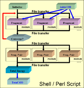
Figure 2: Flow of calculation of the grid-enabled FMO

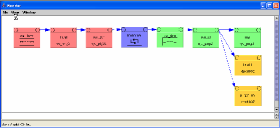
Figure 3: Flow of LC-FMO represented in NAREGI Workflow Tool

We have developed a grid-enabled version of FMO, called a Loosely-coupled (LC) FMO program[8], as part of the NAREGI project. At first, we show the procedure to change the GAMESS-FMO programs into a “loosely-coupled form,” where the original FMO in the GAMESS package is divided into several “single task” modules which are connected each other through input/output file transfers. Those modules consists of run.ini for the initialization, run.mon for the fragment calculation (monomer), run.dim for the fragment pair calculation (dimer), and run.tot for the total energy calculation, and are invoked from a script program which also manages the file transfer over distributed computers. The total flow of the LC-FMO is shown in fig. 2.

Another benefit of the loosely-coupled form is the extendibility of its functionality. In fact, after the first release of the LC-FMO, we have developed two other modules which realize a linkage to the initial density database and a visualization feature of the total molecular orbitals. Since the top-level program to invoke modules is lightweight and can be written in script languages, further modification of the total flow is easily performed.

II-C Execution on NAREGI Grid

In order to execute LC-FMO on the NAREGI grid, we put the flow of the program into NAREGI Workflow Tool[3]. The graphical representation of the LC-FMO program is shown in fig. 3, where modules and input/output files are represented in icons connected each other. This procedure is simple and straightforward because we have already reconstructed the program into a suitable form for distributed computing. Thus, the important is whether the basic structure of the program is grid-aware or not.

Once a program is grid-enabled, we can execute it by the use of the large-scale computing resources over one thousand CPUs. From the programmer’s points of view, the most preferable thing is that we are relieved of arranging the resources to execute the program in high efficiency. In NAREGI testbed system[3], NAREGI Super Scheduler can manage the resource rearrangement with the help of NAREGI Information Service.

II-D Efficiency of LC-FMO

Robustness and efficiency are conflicting each other in general. Since our reconstruction of FMO to increase the controllability might hurt the efficient execution of the program, it is necessary to evaluate the efficiency of LC-FMO by comparing with the original FMO program in GAMESS.

In table I, we show elapsed times for chicken egg white cystatin (1CEW, 1701 atoms, 106 fragments, shown in fig. 4) by the LC-FMO and the original GAMESS-FMO codes. This is obtained on the NAREGI testbed system which consists of 16 CPUs of Xeon 3GHz. Generally speaking, an increase of the total elapsed time is inevitable when we reconstruct some application into a loosely-coupled form, which is considered as a cost for grid-enabling. As shown in table I, however, the increase of the time is relatively small. Thus, it is evaluated that the LC-FMO is effectively executed on grids.

TABLE I: The elapsed time for chicken egg white cystatin.

	LC-FMO	GAMESS-FMO
Initial Guess	37s	4s
Monomer	1h11m	59m
Dimer	2h16m	2h11m
Energy	4s	$<$ 1s
Total	3h28m	3h10m

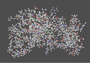
Figure 4: The molecular structure of chicken egg white cystatin (1CEW, 1701 atoms, 106 fragments).

III Performance Prediction

In this section, we predict what performance would be expected if we executed our FMO program in a “peta-scale computer.” Since the actual hardware is not available at present, the prediction is based on a hypothetical specifications of the computer.

III-A Hypothetical Specification of the Peta-scale Computer

It is said that, in a few years, such computer systems with peta-scale specifications will be designed[9]. Here, we concentrate on the CPU resources of the peta-scale computer, and estimate how many CPU resources are necessary to attain peta-scale performances.

The current peak performance of a single-core CPU is the order of 10 giga flops. If a parallel computer with 10 peta-flops peak performance is configured by the CPU to achieve 1 peta-flop effective performance, 1,000,000 CPU cores are necessary in total. Since cluster system constructed by 1,000,000 machines connected each other is unimaginable, it is necessary to rearrange those resources into multiple layers. We do not concern here how to realize computational nodes with multiple CPU cores. If we can configure a lowest layer by a node with the performance of 100 $\sim$ 1,000 CPUs, the total computer will be a parallel system composed of 1,000 $\sim$ 10,000 nodes.

III-B Performance Prediction of FMO

The procedure to predict the performance of FMO in the peta-scale computer is a somewhat phenomenological method based on actual measurements in current computer systems. First, we assume an execution model of FMO which gives a theoretical timing function of the number of fragments $N_{f}$. After fixing some parameters by several measurements of the program, we predict the elapsed time on the virtual computer with peta-scale specifications.

III-B1 Execution Model of GAMESS-FMO

TABLE II: Timing data obtained in a single node of IBM p5 1.9GHz.

Input		1cew	1ao6_half	1ao6	1ao6_dim
No. Atom		1701	9121	18242	36484
$N_{f}$		106	561	1122	2244
$N_{d}(N_{f})$		690	4192	8416	16832
$N_{es}(N_{f})$		4875	152888	620465	2499814
$I_{m}$		17	17	17	17
	monomer	1356	13364	40005	140810
	(Average)	(0.752)	(1.40)	(2.10)	(3.69)
Time	SCF-dimer	2037	20689	70465	186901
(sec)	(Average)	(2.95)	(4.94)	(8.37)	(11.1)
	ES-dimer	398	13772	55955	208627
	(Average)	(0.0816)	(0.0901)	(0.0902)	(0.0835)
Elapsed Time (sec)		3799	47886	166601	536898

TABLE III: Timing data obtained in 16 CPUs of Xeon 3GHz.

Input		1cew	1ao6_half	1ao6
No. Atoms		1701	9121	18242
$N_{f}$		106	561	1122
$N_{d}(N_{f})$		690	4192	8416
$N_{es}(N_{f})$		4875	152888	620465
$I_{m}$		17	17	17
	monomer	1030.4	10808.9	33989.2
	(Average)	(9.72)	(19.3)	(30.3)
Time	SCF-dimer	1677.4	17517.6	50819.2
(sec)	(Average)	(41.3)	(71.0)	(102.7)
	ES-dimer	293.1	9594.8	39133.4
	(Average)	(1.02)	(1.07)	(1.07)
Elapsed Time (sec)		3003.5	38065.9	126330.9

Even if you could analyze all the program codes of GAMESS, it is almost impossible to determine the number of floating-point calculations in a FMO routine precisely since there are many conditional branches which depend on the molecular structure given as an input. Our strategy, here, is a practical approach to obtain phenomenological values of the execution time through experimental executions of FMO in the current machines.

The total execution time of FMO is divided into three parts: a monomer part, an SCF-dimer part, and an ES-dimer part. The monomer and SCF-dimer parts perform SCF calculations for each fragments and each pair of fragments, respectively, while the ES-dimer part obtains dimer correction terms under an electro-static (ES) approximation between fragments. Usually, the ES approximation is applied to the fragment pair with fragments which are separated more than a certain threshold. We start from an expression of the total amount of computation as a function of the number of fragments $N_{f}$,

$$F_{\rm total}(N_{f})=F_{m}(N_{f})+F_{d}(N_{f})+F_{es}(N_{f}),$$ (1)

where $F_{m}(N_{f})$, $F_{d}(N_{f})$, and $F_{es}(N_{f})$ represent the number of floating-point calculations for monomer, SCF-dimer, and ES-dimer parts, respectively. These are assumed as

$$F_{m}(N_{f}) = \left[f_{m}^{(0)}+f_{m}^{(1)}N_{f}\right]N_{f}I_{m}$$ (2)

$$F_{d}(N_{f}) = \left[f_{d}^{(0)}+f_{d}^{(1)}N_{f}\right]N_{d}(N_{f})$$ (3)

$$F_{es}(N_{f}) = f_{es}^{(0)}N_{es}(N_{f}),$$ (4)

according to the algorithm of the FMO theory[4], where $I_{m}$ is the number of monomer loops, $N_{d}(N_{f})$ and $N_{es}(N_{f})$ represent the numbers of SCF-dimers and ES-dimers. SCF calculations for monomers and dimers in FMO depend on the environmental potential which is made by all the fragments other than the target monomer and dimer, while it can be ignored for ES-dimers. Thus, we represent the amount of each SCF calculation for a monomer and an SCF-dimer up to a linear term of $N_{f}$, and that of non-SCF calculation for an ES-dimer as a constant. The parameters, $f_{m}^{(0)}$, $f_{m}^{(1)}$, $f_{d}^{(0)}$, $f_{d}^{(1)}$, $f_{es}^{(0)}$, should be determined from the actual timing data. If we define additional parameters, the number of parallel nodes $K$ and the effective floating-point performance $E$ (flops) of each node, we can compare the actual timing data with the amount of computation divided by $KE$.

Table II and III show the timing data of each part in test executions of several inputs on the machines, 1 node of IBM p5 1.9GHz and a 16 CPU cluster of intel Xeon 3GHz. Since the averaged size of fragments in these inputs are considered as almost the same, the difference of the elapsed time mainly depends on the number of the total fragments $N_{f}$. The least-square fitting with the additional parameters representing the effective performances of each computer, $E_{\rm ibm}$ and $E_{\rm xeon}$, determines all the parameter values shown in table IV after the normalization $E_{\rm ibm}=1$. In figures 5 (a), (b) and (c), we plot the timing data and the results of the functions, (a) $(f_{m}^{(0)}+f_{m}^{(1)}N_{f})/KE$, (b) $(f_{d}^{(0)}+f_{d}^{(1)}N_{f})/KE$, and (c) $f_{es}^{(0)}/KE$.

TABLE IV: Parameter values to represent the execution model of FMO

Parameter		Value
$f_{m}^{(0)}$	$f_{m}^{(1)}$	0.59	0.0014
$f_{d}^{(0)}$	$f_{d}^{(1)}$	2.83	0.0039
$f_{es}^{(0)}$	—	0.082	—
$E_{\rm ibm}$	$E_{\rm xeon}$	1.0	0.071

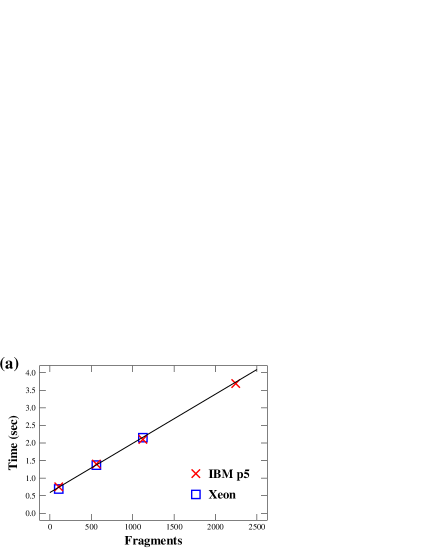
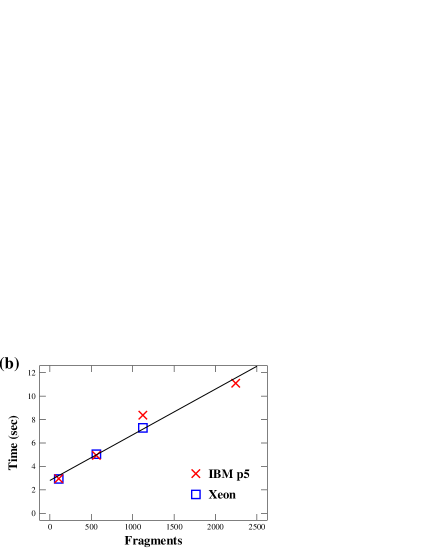
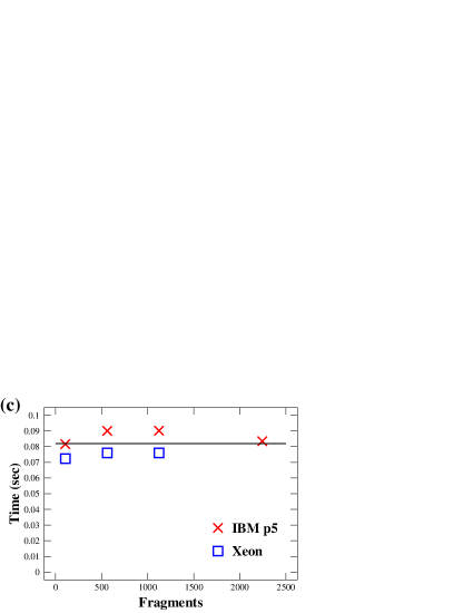
Figure 5: The fragment number dependency of the amount of computation for (a) a monomer, (b) an SCF-dimer, and (c) an ES-dimer are plotted with the effective performance ratios ($E=1$ for IBM p5, $E=0.071$ for Xeon). Lines are functions (a) $(f_{m}^{(0)}+f_{m}^{(1)}N_{f})/KE$, (b) $(f_{d}^{(0)}+f_{d}^{(1)}N_{f})/KE$, and (c) $f_{es}^{(0)}/KE$ obtained by the least-square method.

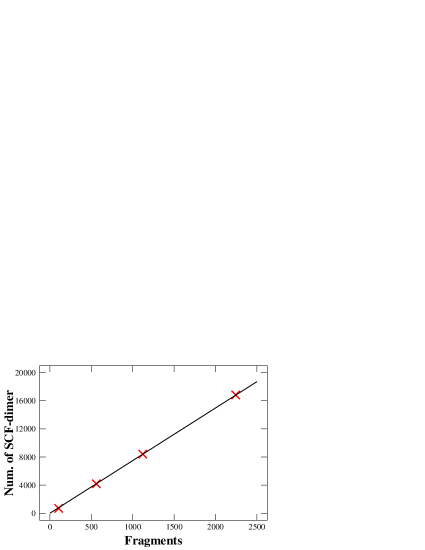
Figure 6: The number of SCF-dimers in the test executions and the function $N_{d}(N_{f})$ by the least-square method.

III-B2 Performance in Peta-scale Computer

In order to predict the total performance of FMO, it is convenient if the functions $N_{d}(N_{f})$ and $N_{es}(N_{f})$ are represented in simple functions of $N_{f}$. By the least-square fitting of the data in table II and III, we obtain a function for the number of SCF-dimers

$$N_{d}(N_{f})=7.50\ N_{f}.$$ (5)

If we consider a constraint

$$N_{d}(N_{f})+N_{es}(N_{f})=\frac{(N_{f}-1)N_{f}}{2},$$ (6)

the number of ES-dimers is represented in the form

$$N_{es}(N_{f})=\frac{(N_{f}-1)N_{f}}{2}-7.50\ N_{f}.$$ (7)

If we substitute these functions and parameters into Eqs. (2), (3), and (4), the total computational amount of FMO is obtained as a function of $N_{f}$. As already seen in the previous section, the FMO algorithm is appropriate for parallel executions when the number of fragments is large enough compared to the number of available nodes. Suppose that we have a peta-scale computer with $K=10000$ and $E=5$, i.e., the number of available nodes is 10,000 and each node has an effective speed 5 times faster than a node of IBM p5 1.9GHz which is used in this paper as a reference machine ($E_{\rm ibm}=1$). Then, the predicted elapsed time $F_{\rm total}(N_{f})/KE$ is calculated as a quadratic function of $N_{f}$ shown in fig. 7. From the viewpoint of the elapsed time, we can perform quantum calculations for molecules with more than 100,000 fragments if the peta-scale computer is realized.

According to the effective performance measurements on PCs, The FMO calculation is executed in 0.5 $\sim$ 1.0 giga flops per one CPU of Xeon or Pentium4, which means that our reference machine, a node of IBM p5 1.9GHz, exhibits almost 10 giga flops for the program since it is $E_{\rm ibm}/E_{\rm xeon}\approx 14$ times faster than a Xeon. Then, the total performance of FMO calculations for a peta computer with $K=10000$ and $E=5$ is considered as 0.5 peta flops. Thus, FMO is considered as a predominant candidate which can record peta-scale performance.

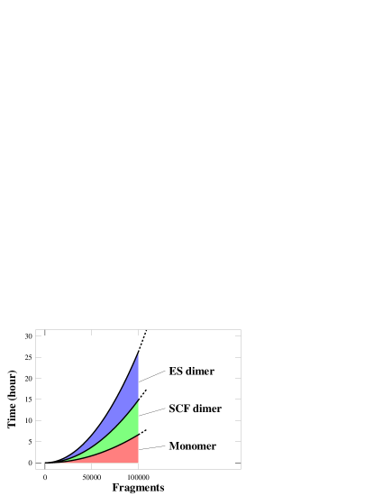
Figure 7: Predicted elapsed time of the FMO calculation by GAMESS as a function of the number of fragments $N_{f}$. This is obtained on the assumption that 10,000 nodes are available, and each node is 5 times faster than a current machine.

IV OpenFMO Project

In spite of the fact that the FMO is a suitable algorithm to achieve the peta-scale performance through large-scale parallel executions, the actual GAMESS-FMO code cannot be executed for the molecule with more than 100,000 fragments. One of the reason why the current program fails to run is memory consumption in each node, where the current FMO code in GAMESS tries to allocate two-dimensional arrays with respect to fragments, e.g., the distance between two fragments. This exceeds 40 giga bytes even if we consider the symmetry. The limit of the number of fragment is considered as the order of 10,000 in the current implementation. Thus, the reconstruction of the FMO code is necessary in order to correspond to the peta-scale computing.

In this section, we introduce our new project to reconstruct a FMO program from scratch. The name of this project, OpenFMO[10], stands for the following openness: (1) names and argument lists of APIs constructing the FMO program are opened publicly, (2) the program structure is also opened to combining other theories of physics and chemistry, i.e., multi-scale/multi-physics simulations, and (3) the skeleton program is developed under some open-source licenses and its development process will also be opened to the public. In fig. 8, we show a stack structure of this program. Although the main target is still a quantum chemical calculation of molecules, it can be combined with other theories to construct multi-physics/multi-scale simulations (fig. 9) for complex phenomena[11].

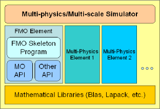
Figure 8: Multi-physics/multi-scale simulator stack including OpenFMO.

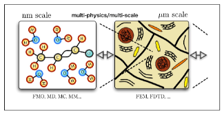
Figure 9: Can multi-physics/multi-scale simulations reveal the true aspect of the complex world of matter?

IV-A Open Architecture Implementation of FMO

As already shown in section II-A, the fragment MO method consists of the standard ab initio MO calculations including the generation of Fock matrices with one/two-electron integral calculations. Using this property, the usual FMO program is divided into two layers, the skeleton program which control the whole flow of the FMO algorithm, and the molecular orbital (MO) APIs to provide the charge distribution of each fragment through ab initio MO calculations. Since these spec of interfaces between the skeleton and the APIs are fixed and opened publicly, either of them can easily be substituted by other programs.

IV-B Open Interface to Multi-physics Simulations

The multi-physics simulation is one of the predominant strategy to construct peta-performance applications for nano-scale materials. Our new implementation of FMO can also be opened for such multi-physics simulations. Since the FMO method is based on electro-static interaction between fragments, we can extend each fragment to the general object which can provide a static charge distribution. For examples, we often use molecular mechanics representation of atomic clusters which should be given by quantum mechanical description, or the environmental charge distribution surrounding a molecule which models a solvent can be included as a fragment. Thus, the MO-APIs for a certain fragment can be substituted to other programs based on the different approximation levels.

In addition to the description in molecular sciences, this is extended to larger-scale simulations through the “multi-physics/multi-scale simulator” layer. This type of extension is widely used for the large-scale computation representing realistic models of molecules in cells or other living organisms.

IV-C Open Source Development of the Programs

The source code of the skeleton program of OpenFMO is publicly opened according to some open-source licenses. At present, the OpenFMO project is managed by several core members including the authors of this paper. Once we show the effectiveness of our approach to the open implementation, and the direction of the project is settled properly, we are willing to change the management of the project into so-called open-source-software developments.

V Summary and Discussion

In this paper, we showed our results in nanoscience executed on the NAREGI grid system, and expressed our perspective toward the peta-scale computing. In section III, we showed that FMO is one of the peta-scale applications. However, it has been also realized that the actual implementations of the FMO method, at present, does not correspond to the execution in peta-scale environments, i.e., they does not solve molecules with more than 10 thousand fragments even if peta-scale computers are available. In order to improve the situation, we started an open-source project for multi-physics simulations including new FMO codes from scratch.

Generally speaking, it is very difficult for scientific applications to be executed in a peta-scale performance since a simple parallel scheme fails in case that the total number of CPUs is the order of 1,000,000. Thus, it will be necessary that the application itself becomes multi-layered in order to use the resources efficiently corresponding to the hardware architecture of peta-scale computers. The FMO calculation which we have studied in this paper has a two-stage structure in its original algorithm: ab initio calculations are performed for each fragment and fragment pair while the interactions between these fragments are described by a classical electro-static potentials. This theoretical reconstruction of the original ab initio MO method into the layered form is considered as the key to the successful performance of the program.

Scientific calculations with layered structures have been carried out as a multi-physics/multi-scale simulation in various fields. This type of calculations is important not only as a technique of realistic simulations but also as an actual example for the peta-scale computing. However, we claim that the deep understanding of the physical/chemical theories must be necessary for a proper construction of effective simulations which describes complex aspects of nature. Then, the theoretical and practical way of constructing such simulations should be established before the time when the peta-scale computers are available. We expect that our implementation of the simulator is one of the solutions for high-performance scientific simulations in the next-generation.

References

- [1] The recent activities for peta-scale computing in Japan are reviewed in “The 11th ‘Science in Japan’ Forum” (Washington DC, Jun 16, 2006), http://www.jspsusa.org/FORUM2006/Agenda06.html
- [2] NAREGI Poject, http://www.naregi.org/
- [3] S. Matsuoka, S. Shimojo, M. Aoyagi, S. Sekiguchi, H. Usami, and K. Miura, “Japanese Computational Grid Research Project: NAREGI,” in Proc. IEEE, 2005, vol. 93, pp. 522–533.
- [4] K. Kitaura, E. Ikeo, T. Asada, T. Nakano, M. Uebayasi, “Fragment Molecular Orbital Method: an Approximate Computational Method for Large Molecules,” Chem. Phys. Lett., 1999, vol. 313, pp. 701–706.
- [5] C. C. J. Roothaan, “New Developments in Molecular Orbital Theory,” Rev. Mod. Phys., 1951, vol. 23, pp. 69–89.
- [6] http://www.msg.ameslab.gov/GAMESS/GAMESS.html
- [7] T. Nakano, T. Kaminuma, T. Sato, K. Fukuzawa, Y. Akiyama, M. Uebayasi, K. Kitaura, “Fragment molecular orbital method: use of approximate electrostatic potential,” Chem. Phys. Lett., 2002, vol. 351, pp. 475.
- [8] M. Aoyagi, “Loosely Coupled Approach on Nano-Science Simulations,” an oral presentation given in “The 11th ‘Science in Japan’ Forum,” http://www.jspsusa.org/FORUM2006/aoyagi-slide.pdf
- [9] Riken Supercomputer Project, http://www.nsc.riken.jp/
- [10] OpenFMO Project, http://www.openfmo.org/
- [11] T. Takami, J. Maki, J. Ooba, T. Kobayashi, R. Nogita, and M. Aoyagi, “Interaction and Localization of One-Electron Orbitals in an Organic Molecule: Fictitious Parameter Analysis for Multiphysics Simulations,” J. Phys. Soc. Jpn. 76, 013001 (2007) [4 pages]; e-print nlin.CD/0611042.