Statistical Keyword Detection in Literary Corpora

Abstract

Understanding the complexity of human language requires an appropriate analysis of the statistical distribution of words in texts. We consider the information retrieval problem of detecting and ranking the relevant words of a text by means of statistical information referring to the spatial use of the words. Shannon’s entropy of information is used as a tool for automatic keyword extraction. By using The Origin of Species by Charles Darwin as a representative text sample, we show the performance of our detector and compare it with another proposals in the literature. The random shuffled text receives special attention as a tool for calibrating the ranking indices.

1 Introduction

Data mining for texts is a well-established area of natural language processing MS99 . Text mining is the computerised extraction of useful answers from a mass of textual information by machine methods, computer-assisted human ones, or a combination of both. A key problem in text mining is the extraction of keywords from texts for which no a priori information is available. The problem of unsupervised extraction of relevant words from their statistical properties was first addressed by Luhn Luh58 , who based his method on Zipf’s analysis of frequencies Zipf . This analysis consists of counting the number of occurrences of each distinct word in a given text, and then generating a list of all these words ordered by decreasing frequency. In this list, each word is identified by its position or Zipf’s rank in the list. The empirical observation of Zipf was that the frequency of occurrence of the $r$–th rank in the list is proportional to $r^{-1}$ (Zipf’s law). Luhn proposed the crude approach of excluding the words at both ends of the Zipf’s list and considering as keywords the remaining cases. The limitations of Luhn’s approach are known in the literature SM83 .

The main goal of this work is to investigate unsupervised statistical methods for detecting keywords in literacy texts beyond the simple counting of word occurrences. In order to obtain statistically significant results we restrict our work to a large book, which can be used as a corpus what is thematically consistent throughout its entire length. We are searching for relevance according to the text’s context, but we will only use statistical information about the spatial use of the words in a text.

Particularly, the measure of content of information for each word can be made by Shannon’s entropy. In the physics literature, we can find several applications of the entropy concept to linguistics and natural language like DNA sequences analysis MBG+95 ; SBG+99 ; GBC+02 , long-range correlations measurements EP94 ; EPA95 , language acquisition CCGG99 , authorship disputes CMH97 ; YPYG03 , communication modelling Can05 , and statistical analysis of the linguistic role of words in corpora MZ02 .

The organisation of the remainder of the article is as follows. In Sec. 2 we first introduce the corpus used as a representative sample throughout this work. Later, in Sec. 3 we review the algorithms proposed in the literature based on the analysis of the statistical distribution of words in a text. Then, in Sec. 4 we discuss the behaviour of the indices in random texts. By using Shannon’s entropy, in Sec. 5 we propose another index based on the information content of the sequence of occurrences of each word in the text. In Sec. 6 we use the glossary of the corpus for measuring the performace of each index as keyword detector. Finally, in Sec. 7 we present a summary of the work. Besides, mathematical details are given in appendices. In Appendix A we review the geometrical distribution, useful to random texts, and in Appendix B we calculate the entropy of a random text.

2 Representative Corpus Sample

For our study, we will use a prototypical real text, i.e., “On the Origin of Species by Means of Natural Selection, or The Preservation of Favoured Races in the Struggle for Life” Gut (usually abbreviated to The Origin of Species) by Charles Darwin (1859). The book was written with the vocabulary of a nineteenth-century naturalist but with fluid prose, combining first–person narrative with scholarly analysis.

For the preparation of our working corpus we first withdrew any punctuation symbol from the text, mapped all words to uppercase and then used the simple tokenization method based on whitespaces MS99 . We draw a distinction between a word token versus a word type. For our convenience, we define a word type as any different string of letters between two whitespaces. Thus, for our elementary analysis, words like INSTINCT and INSTINCTS correspond to different word types in our corpus. On the other hand, a word token is each individual occurrence of a given word type. When the context refers to a particular word type, we will use indistinctly “word token” or simply “token” to refer to an individual occurrence of the word type in the text.

The relevant words have not been explicitly defined in Darwin’s book, with exception of a glossary appended at the end of the work. Therefore, the table of contens in the beginning, the glossary and the analytical index, also inserted at the end, were removed from our corpus. By doing this, we avoid introducing obvious bias for the words used in these parts. Thus, the prepared corpus includes $94\%$ of material from the original Darwin’s book and has $192,665$ word tokens and $8,294$ word types. In addition, the corpus contains $842$ paragraphs distributed in $16$ chapters.

The glossary of the principal scientific terms used in the book, prepared by Mr. W.S. Dallas, and the analytical index, both appended at the end of the book, were written using $2,418$ word types. If we do not consider the function words, still remain $1,679$ word types ($20\%$ of the book’s lexicon). With this information,, we prepared by hand a customed version of the glossary, by selecting $283$ word types ($3.4\%$ of the lexicon) with frequencies of occurrence greater than 9. We have avoided word types with less than 9 occurrences because we cannot extract any significant statistics from data obtained using such small sets. Thus, the criterion for selection was rather more arbitrary, but we think that all selected words are pertinent to the book’s context. Our prepared version of the glossary will be used later to evaluate the retrieval capabilities of different keyword extractors.

3 Clustering as criterion for relevance of words

The attraction between words is a phenomenon that plays an important role in both language processing and acquisition, and it has been modeled for information retrieval and speech recognition purposes BBL97 ; NW97 . Empirical data reveals that the attraction between words decays exponentially, while stylistic and syntactic constraints create a repulsion between words that discourages close occurrences. In Fig. (1) we have plotted the histogram of absolute frequencies of distances between nearest neighbour tokens of the word type NATURAL in Darwin’s corpus. For long distances, Fig. (1) qualitatively suggests an exponential tail, but for very short distances the frequencies decay abruptly. Also in Fig. (1) we have superimposed the histogram of a random shuffled version of the corpus where we can qualitatively see an exponential decay for all distances.

Figure 1: Histogram of frequencies of distances between occurrences of NATURAL (Zipf’s rank 53) in Darwin’s corpus.

The attraction–repulsion phenomenon is more emphasized for relevant words than for common words, which have less syntactic penalties for close co-occurrence. Therefore, the spatial distributions of relevant words in the text are inhomogeneous and these words gather together in some portions of the text forming clusters. The clustering phenomenon can be visualised in Fig. 2 where we have plotted the absolute positions of four different word types from Darwin’s corpus in a “bar code” arrangement. The clustering becomes manifest in the patterns of NATURAL, LIFE, and INSTINCT in spite of their different numbers of occurrences. In contrast, THE (the more frequent word in the English language) has no apparent clustering.

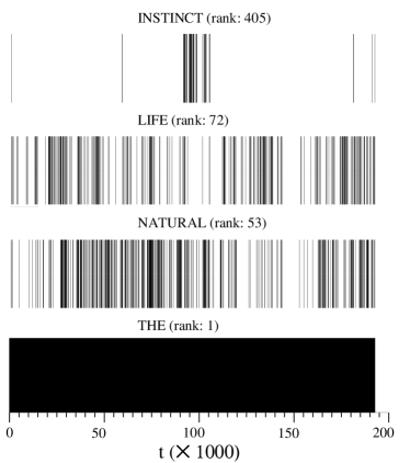
Figure 2: Absolute positions ($t$) in the text, counted from the beginning of Darwin’s corpus, of the word types: THE ($13,414$ occurrences), NATURAL ($475$ occurrences), LIFE ($326$ occurrences), and INSTINCT ($64$ occurrences). To draw the picture, we set a very thin vertical line (of arbitrary height) at the position of each occurrence.

Recently, the assumption that highly relevant words should be concentrated in some portions of the text was used for searching relevant words in a given text. In the following two subsections, we briefly review the indices of relevance of words proposed by Ortuño et al. OCB+02 and Zhou and Slater ZS03 , which are based on the spatial distribution of words in the text.

3.1 $\sigma$–index

To study the spatial distribution of a given word type in a text, we can map the occurrences of the corresponding word tokens into a time series. For this task, we denote by $t_{i}$ the absolute position in the corpus of the $i$–th occurrence of a word token. Thus, we obtain the sequence $\{t_{0},t_{1},\dots,t_{n},t_{n+1}\}$, where we are assuming that there are $n$ word tokens. We have additionally included the boundaries of the corpus, defining $t_{0}=0$ and $t_{n+1}=N+1$, where $N$ is the total number of tokens in the corpus, in order to take into account the space before the first occurrence of a word token and the space after the last occurrence of a token ZS03 .

Given the sequence of inter–token distances

$$\{t_{1}-t_{0},t_{2}-t_{1},\dots,t_{n}-t_{n-1},t_{n+1}-t_{n}\}\,,$$

the average distance between two successive word tokens is given by

$$\mu=\frac{1}{n+1}\,\sum_{i=0}^{n}\left(t_{i+1}-t_{i}\right)=\frac{N+1}{n+1}\;,$$ (1)

and the sample standard deviation of the set of spacings between nearest neighbour word tokens ($t_{i+1}-t_{i}$) is by definition

$$s=\sqrt{\frac{1}{n-1}\,\sum_{i=0}^{n}\left((t_{i+1}-t_{i})-\mu\right)^{2}}\;.$$ (2)

To eliminate the dependence on the frequency of occurrence for different word types, in Ref. OCB+02 the authors suggest to normalise the token spacings, i.e., to measure them in units of their corresponding mean value. Thus, we define

$$\sigma=\frac{s}{\mu}\;.$$ (3)

Given that the standard deviation grows rapidly when the inhomogeneity of the distribution of spacing $t_{i+1}-t_{i}$ increases, Ortuño et al. OCB+02 proposed $\sigma$ as an indicator of the relevance of the words in the analysed text. In many cases, empirical evidence vindicates that large $\sigma$ values generally correspond to terms relevant to the text considered, and that common words have associated low values of $\sigma$. However, Zhou and Slater ZS03 pointed out that $\sigma$-index has some weaknesses. First, several obviously common (relevant) words have relative high (low) $\sigma$ values in several texts. Second, the index is not stable in the sense that it can be strongly affected by the change of a single occurrence position. Third, high values of $\sigma$ do not always imply a cluster concentration. A big cluster of words can be splitted into smaller clusters without substantial change in the $\sigma$ value.

3.2 $\Gamma$–index

The $\sigma$-index is only based on the spacing between nearest-neighbour word tokens. To improve the performance in the searching for relevance, Zhou and Slater ZS03 introduced a new index that uses more information from the sequence of occurrences $\{t_{0},t_{1},\dots,t_{n},t_{n+1}\}$. For this task, these authors consider the spacings $w_{i}=t_{i}-t_{i-1}$, with $i=1,\dots,n+1$, and define the average separation around the occurrence at $t_{i}$ as

$$d(t_{i})=\frac{w_{i+1}+w_{i}}{2}=\frac{t_{i+1}-t_{i-1}}{2},\qquad i=1,\ldots,n\,.$$ (4)

The position $t_{i}$ is said to be a cluster point if $d(t_{i})<\mu$. The new suggestion is that the relevance of a word in a given text is related to the number of cluster points found in it. Thus, in order to measure the degree of clusterization, the local cluster index at position $t_{i}$ is defined by

$$\gamma(t_{i})=\left\{\begin{array}[]{lcl}\displaystyle\frac{\mu-d(t_{i})}{\mu}&&\textrm{ if $t_{i}$ is a cluster point}\\ 0&&\textrm{ otherwise}\end{array}\right.\;.$$ (5)

Finally, a new index to measure relevance is obtained from the average of all cluster indices corresponding to a given word type

$$\Gamma=\frac{1}{n}\sum_{i=1}^{n}\gamma(t_{i})\;.$$ (6)

$\Gamma$-index is more stable than $\sigma$, but it is still based on local information and is computationally more time consuming to evaluate than $\sigma$.

4 Random text and shuffled words

In a completely random text we have an uncorrelated sequence of tokens, and a word type $w$ is only characterised by its relative frequency of occurrence ($p_{w}$). Thus, a random text can be generated by picking successively tokens by chance in such a way that at each position the probability of finding a token, corresponding to the word type $w$, is $p_{w}$. Obviously, $\sum_{w}p_{w}=1$. For the word type $w$, we have in this manner defined a binomial experiment where the probability of success (occurrence) at each site in the text is $p_{w}$, and the probability of failure (non-occurrence) is $(1-p_{w})$. Therefore, the distribution of distances between nearest neighbour tokens corresponding to the same word type is geometrical. In Appendix A, we have compiled some results of the geometrical distribution that are useful for our next analyses.

Besides, its worth as comparative standard, the theoretical random text has the virtue of being analytically tractable. Also, from an empirical point of view, there is a workable fashion for building a random version of a corpus. In an actual corpus the probabilities of occurrence $p$ are estimated from the relative frequencies $n/N$, where $n$ is the number of tokens corresponding to a given word type and $N$ is the total number of tokens in the corpus. A random version of the text can be obtained by shuffling or permuting all the tokens. The random shuffling of all the words has the effect of rescasting the corpus into a nonsensical realization, keeping the same original tokens without discernible order at any level. However, both the Zipf’s list of ranks and the frequency of occurrence of each word type are kept intact.

The important point that we want to stress here is that the indices of relevance defined in the previous section are functions of the frequencies of occurrence of each word type. Thus, in a random text the values of these indices change with $p$, which has nonsense. In a truly random text, there are not relevant words. Therefore, to eliminate completely the dependence on frequency we need to renormalise the indices with their values in the random version of the corpus.

4.1 Renormalised $\sigma$–index

For a given probability distribution, $\sigma$ is defined from the second– ($\mu_{2}$) and first–order ($\mu_{1}$) cumulant by $\sqrt{\mu_{2}}/\mu_{1}$. Thus, from Eq. (20) in Appendix A we find that in a random text the value of $\sigma$–index is given by

$$\sigma_{\mbox{ran}}=\sqrt{1-p}\;.$$ (7)

Hence, we renormalise the index to eliminate this dependence on relative frequency defining

$$\sigma_{\mbox{nor}}=\frac{s}{\mu}\frac{1}{\sqrt{1-p}}\;.$$ (8)

For texts as large as corpora the importance of normalisation factor given by Eq. (7) becomes negligible. For example, in Darwin’s corpus, $N=192,665$, and for the most frequent word type (THE) we have $n=13,414$ ($n/N=0.0696$). Thus, in the less significant case (the lowest value for $\sigma_{\mbox{ran}}$) $\sigma_{\mbox{ran}}=0.965$, whereas $\sigma_{\mbox{ran}}=1$ for $p=0$. However, for shorter texts the significance of the normalisation may become critical and the values of $\sigma$ and $\sigma_{\mbox{nor}}$ may be very different for any word type.

In Fig. 3 we plot the values of $\sigma_{\mbox{nor}}$ for the first $4000$ ranks in the Zipf’s list of Darwin’s corpus. The random version of the corpus is also plotted in the same graph. The “cloud of points” corresponding to the random text is distributed around the unitary value of $\sigma_{\mbox{nor}}$, but the width of the “cloud” grows with rank. This behaviour is due to the fact that the frequency of occurrence decreases as the rank increases (Zipf’s law), therefore the statistics get worse. The words of our preparated version of the glossary are marked by open circles in Fig. 3. From Fig. 3, it is appreciable that most of the glossary words have high values of $\sigma_{\mbox{nor}}$.

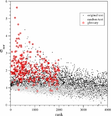
Figure 3: Renormalised $\sigma$–index vs. Zipf’s rank for each word in Darwin’s corpus (the first 4000 ranks). We have also plotted superposed the random version of the text (grey) and we have marked by open circles the words corresponding to our prepared glossary (red online).

4.2 Renormalised skewness

As in the case of $\sigma$, any cumulant contains partial information of the spatial distribution of words. Skewness is a parameter that describes the asymmetry of a distribution. Mathematically, the skewness is measured using the second– ($\mu_{2}$) and third–order ($\mu_{3}$) cumulant of the distribution according to $\kappa=\mu_{3}/\mu_{2}^{3/2}$. Given that the distances between nearest neighbour tokens are positive defined, the corresponding distribution has positive skew, i.e., the upper tail is longer than the the lower tail (see Fig. 1).

From Eq. (20), we find that in a random text the skewness of the distribution of distances between nearest neighbour tokens is given by

$$\kappa_{\mbox{ran}}=\displaystyle\frac{2-p}{\sqrt{1-p}}\;;$$ (9)

Thus, the skewness also depends on the relative frequency of occurrence, $p$, in the random case. However, this dependence is also negligible for a corpora. In Darwin’s corpus we obtain $\kappa_{\mbox{ran}}=2.001$ for the largest value $p=0.0696$ (the relative frequency of the word type THE), whereas $\kappa_{\mbox{ran}}=2$ for $p=0$.

As a consequence, we can define another renormalised quantity as we did with the $\sigma$–index. Thus, to eliminate the dependence on the relative frequency of occurrence in the random case, we write

$$\kappa_{\mbox{nor}}=\frac{\mu_{3}}{\mu_{2}^{3/2}}\frac{\sqrt{1-p}}{2-p}\;.$$ (10)

$\kappa_{\mbox{nor}}$ can also be used for measuring relevance. However, the finite-size effects of the texts are more pronounced for higher order cumulants. We now use both cumulants $\sigma_{\mbox{nor}}$ and $\kappa_{\mbox{nor}}$ to construct a bi-dimensional graph for the corpus. In this manner, in Fig. 4 we plot the the pairs $(\sigma_{\mbox{nor}},\kappa_{\mbox{nor}})$ for all words in Darwin’s corpus. In this graph, the “cloud of points” corresponding to the random text is distributed around the pair of values $(1,1)$, while the region defined by $\sigma_{\mbox{nor}}>2$ and $\kappa_{\mbox{nor}}>2$ has almost none. The upper right corner of the graph concentrates almost all the points corresponding to the glossary.

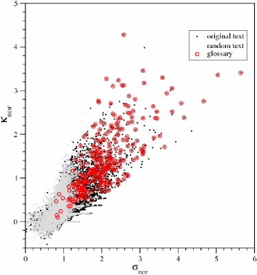
Figure 4: Renormalised $\kappa$–index vs. $\sigma$–index for all words in Darwin’s corpus. We have also plotted superposed the random version of the text (grey) and we have marked by open circles the words corresponding to our prepared glossary (red online).

Figure 4 gives us immediate insight into the distribution of distances between nearest neighbour tokens, and provides us a powerful tool for determining keywords.

4.3 Renormalised $\Gamma$–index

As we did with the $\sigma$–index, we need to calculate $\Gamma$ for a word type which appears in a random text with relative frequency $p$. For this task, we calculate the average of the random variable $\gamma$ defined in Eq. (5) in a random text. From Eq. (30) in Appendix A we obtain

$$\Gamma_{\mbox{ran}}=\displaystyle\frac{1}{2}\,h\,(h-1)\,(1-p)^{h}\,((1-p)+(1-p)^{-1}-2)\;,$$ (11)

where $h=\mbox{Int}[2/p]$. In this case, the dependence on $p$ is even more complicated than previous cases. This observation is absent from Ref. ZS03 . Zhou and Slater only calculate the value of $\Gamma$ for the Poisson distribution: $\Gamma=2\,e^{-2}$ (see Eq. (33) in Appendix A), which is constant ($\approx 0.271$). Also in this case, the dependence on $p$ is negligible for corpora. In Darwin’s corpus we obtain $\Gamma_{\mbox{ran}}=0.261$ for the largest value of $p=0.0696$ (the relative frequency of the word type THE), whereas $\Gamma_{\mbox{ran}}\approx 0.271$ in the limit $p\rightarrow 0$ (see Appendix A).

Now, as in the other cases, we define from Eqs. (6) and (11) a renormalised index by $\Gamma_{\mbox{nor}}=\Gamma/\Gamma_{\mbox{ran}}$. In Fig. 5 we plot the values of $\Gamma_{\mbox{nor}}$ for the first $4000$ ranks in the Zipf’s list of Darwin’s corpus. The “cloud of points” corresponding to the random text is distributed around the unitary value, but the width of the “cloud” grows with rank faster than in the case of $\sigma_{\mbox{nor}}$. The words corresponding to the glossary have systematically high values of $\Gamma_{\mbox{nor}}$.

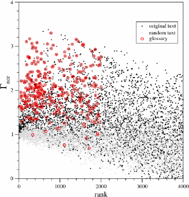
Figure 5: Renormalised $\Gamma$–index vs. Zipf’s rank for each word in Darwin’s corpus (the first 4000 ranks). We have also plotted superposed the random version of the text (grey) and we have marked by open circles the words corresponding to our prepared glossary (red online).

5 Entropy of token distributions

Claude Shannon introduced the concept of entropy of information in 1948 SW49 . Mapping a discrete information source on a set of possible events whose probabilities of occurrences are $p_{1},p_{2},\dots,p_{P}$, Shannon constructed a measure of information and uncertainty, $S(p_{1},p_{2},\dots,p_{P})$, requiring the following properties:

1. $S$ should be continuous in the $\{p_{i}\}$.

2. For the iso-probability case, $p_{i}=1/P$, $S$ should be a monotonic increasing function of $P$.

3. If the set $p_{1},p_{2},\dots,p_{P}$ is broken down into two subsets with probabilities $w_{1}=p_{1}+\dots+p_{k}$ and $w_{2}=p_{k+1}+\dots+p_{P}$, then we must have the following composition law $S(p_{1},\dots p_{N})=S(w_{1},w_{2})+w_{1}\,S(p_{1}/w_{1},\dots p_{k}/w_{1})\\ +w_{2}\,S(p_{k+1}/w_{2},\dots p_{P}/w_{2})$.

The only $S$ satisfying the three above assumptions is of the form

$$S(p_{1},p_{2},\dots,p_{P})=-K\sum_{i=1}^{P}p_{i}\,\log p_{i}\,,$$ (12)

where $K$ is a positive constant.

A literary corpus can be divided in parts using natural partitions such as parts, sections, chapters, paragraphs or sentences. Thus, we consider the corpus as a composite of $P$ parts. For the $i$–th part of the corpus we can reckon up the total number $N_{i}$ of tokens and the number $n_{i}(w)$ of occurrence of the word type $w$ inside this part. Then, the fraction $f_{i}(w)=n_{i}(w)/N_{i}$ ($i=1,\dots,P$) is the relative frequency of occurrence of the word type $w$ in the part $i$. Obviously, $\sum_{i=1}^{P}N_{i}=N$ is the total number of tokens in the corpus and $\sum_{i=1}^{P}n_{i}(w)=n(w)$ is the number of tokens corresponding to the word type $w$. Therefore, it is possible to define a probability measure over the partitions MZ02 as

$$p_{i}(w)=\frac{f_{i}(w)}{\displaystyle\sum_{j=1}^{P}f_{j}(w)}\;.$$ (13)

The quantity $p_{i}(w)$ results more complex than the conditional probability $f_{i}(w)/(n(w)/N)$, of finding the word type $w$ in the part $i$ given that it is present in the corpus.

Following Shannon’s arguments, the information entropy associated with the discrete distribution $p_{i}(w)$ is

$$S(w)=-\frac{1}{\ln(P)}\sum_{i=1}^{P}p_{i}(w)\ln(p_{i}(w))\;.$$ (14)

The value $1/\ln(P)$ for the constant $K$ was selected to take the maximum value of $S$ equal to one. Thus, $0<S(w)<1$. In this manner, when a type word is uniformly distributed ($p_{i}=1/P$, for all $i$), Eq. (14) yields $S=1$. Conversely, the other extreme case, $S=0$, is when a word type appears only in part $j$, thus we have $p_{j}=1$ and $p_{i}=0$ for $i\neq j$. Therefore, words with frequent grammatical use like function words (prepositions, adverbs, adjectives, conjunctions, and pronouns) will have high values of entropy, meanwhile keywords will have low values of entropy. Empirical evidence MZ02 shows a tendency of the entropy to increase with $n$. It implies that, on average, the more frequent word types are more uniformly used.

As we did with preceding indices, we need to calculate the average of the entropy of a mock word type that appears $n$ times in a random corpus. From Eq. (39) in Appendix B, we obtain

$$(1-S)_{\mbox{ran}}\approx\frac{P-1}{2\,n\,\ln P}\,,$$ (15)

for $n>>1$ and if all the parts of the random text have the same number of tokens. Empirical evidence MZ02 shows that the agreement of Eq. (15) with random shuffling of texts using natural partitions is very good, in spite of the limitation of the last assumption. From Eq. (15), we can see that the dependence on the absolute frequency, $n$, is critical for $(1-S)_{\mbox{ran}}$ and it could not be ignored even if the text is as large as a corpus.

Montemurro and Zanette MZ02 proposed Eqs. (13) and (14) to study the distribution of words according to their linguistic role. For this task, they found that the suitable coordinates whereby words can be categorized are $n\,(1-S)$ and $n$. In the same way, we will use these ideas for detecting relevance of words. We cannot use directly the entropy as index because all tokens with only one occurrence have zero entropy. Thus, we define a normalised index freed from the dependence on absolute frequency ($n$) in random texts by

$$E_{\mbox{nor}}(w)=n(w)\,(1-S(w))_{\mbox{nor}}=n(w)\frac{2\,\ln P}{P-1}\,(1-S(w))\,.$$ (16)

Figure 6 shows the values of $E_{\mbox{nor}}$ for all word types of Darwin’s corpus versus its number of occurrence, $n$, on a double logarithmic scale. The individual deviations from the bulk trend for each value of $n$ are related to the particular usage nuances of words. To stress these deviations, we have used the 16 chapters of the corpus as natural partitions for our entropic analysis (i.e. $P=16$). In this way, we obtain a remarkable scattering of higher values of $E_{\mbox{nor}}$ in the full range of number of occurrences. A same entropic analysis using the $842$ paragraphs of Darwin’s corpus as partitions (i.e. $P=842$) generates a similar graph that stresses the bulk trend, but the fluctuations are completely smoothed. Using the chapters as partitions ($P=16$) in Fig. 6, the “cloud of points” corresponding to the random version of the corpus is distributed around the unitary value and the corpus appears clearly more separated from the random text than with previous indices. Additionally, the words corresponding to the glossary have systematically high values of the index $E_{\mbox{nor}}$.

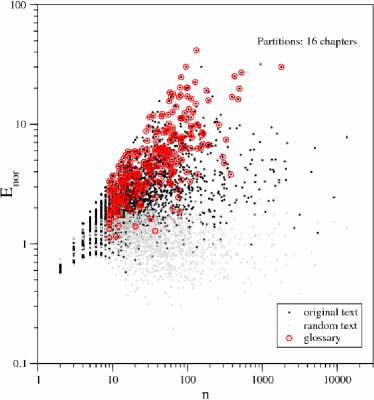
Figure 6: $E_{\mbox{nor}}$ vs. number of occurrence ($n$) for each word in Darwin’s corpus. We have also plotted superposed the random version of the corpus (grey) and we have marked by open circles the words corresponding to our prepared glossary (red online).

To reinforce our graphical findings, in the following section we perform a quantitative comparison among the indices $\sigma_{\mbox{nor}}$, $\kappa_{\mbox{nor}}$, $\Gamma_{\mbox{nor}}$, and $E_{\mbox{nor}}$ based on the power of each index for discriminating the glossary from the bulk of words.

6 Glossary as benchmark

Evaluation in information retrieval makes frequent use of the notions of recall and precision MS99 ; SM83 . Recall is defined as the proportion of the target items that a system recover. Precision is defined as a measure of the proportion of selected items that are targets. Remembering that our prepared glossary has $283$ word types, we denote by $NG$ the number of the glossary’s word types among the first top $283$ ranked word types of the corpus. For our purposes, we define recall of an index of relevance as the fraction $NG/283$. Thus, recall for the index $E_{\mbox{nor}}$ results $41\%$. On the other hand, precision can be built looking for the last word type of our prepared glossary in the global ranking of each index. For our convenience, we denote by $LP$ the position in the ranking of the last word type of the glossary, and we define precision of a keyword extractor as the fraction $283/LP$. Thus, for example, the last entry of the glossary according to the index $E_{\mbox{nor}}$ is FLOWERING and is ranked in the position $2,790$. Remembering that the corpus has $8,294$ word types, we obtain that the complete prepared glossary is allocated by $E_{\mbox{nor}}$ in the first third part of the ranked lexicon and the precision of the index results $10\%$. Recall and precision are useful benchmarks for measuring the index’s performance. In particular, recall and precision of each index analysed in this work are given in Table 1. We want to stress that the values of recall and precision of the indices $\sigma$ and $\Gamma$ are exactly the same as those obtained for $\sigma_{\mbox{nor}}$ and $\Gamma_{\mbox{nor}}$, respectively. This fact is due to the normalisation factors given by Eqs. (7) and (11), which are almost constant for a corpus. Therefore, the pair of indices $\sigma$ and $\sigma_{\mbox{nor}}$ (or $\Gamma$ and $\Gamma_{\mbox{nor}}$) yield identical rankings of keywords.

Table 1: Recall and precision of each index. $NG$ is the number of glossary’s word types among the first $283$ entries of each ranking. $LP$ is the last position in each ranking in which appears a word type of the glossary. Thus, recall $=NG/283$ and precision = $283/LP$.

Index	$NG$	recall	$LP$	precision	last word
$E_{\mbox{nor}}$	118	0.417	$2,790$	0.101	FLOWERING
$\sigma_{\mbox{nor}}$	114	0.403	$5,689$	0.050	SCARCELY
$\kappa_{\mbox{nor}}$	107	0.378	$4,181$	0.068	INDIAN
$\Gamma_{\mbox{nor}}$	72	0.254	$4,312$	0.066	OSTRICH

In order to compare the performance of all indices, in Fig. 7 we have drawn a precision–recall plot where we can see the significant improvement performed by the index $E_{\mbox{nor}}$, both in recall and precision. Also, in Fiq. (7) we see that $\kappa_{\mbox{nor}}$ has a recall slightly worse than $\sigma_{\mbox{nor}}$ and precision as good as $\Gamma_{\mbox{nor}}$. Thus, we find that the skewness of the distribution of occurrences of a word type has a significant part of information about the relevance of the word in the text.

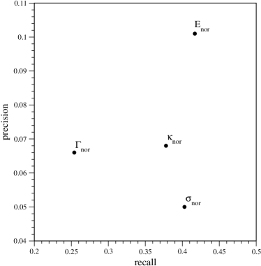
Figure 7: Comparison of information retrieval performance of the indices (see Table 1).

In Table 2 we show the first top 50 word types of the prepared glossary ranked by the index $E_{\mbox{nor}}$. We also show the rank position of each word type by the others indices.

Table 2: First top 50 word types of the prepared glossary ranked by the index $E_{\mbox{nor}}$. The numerical values correspond to the positions in the ranking of each word type, not to the actual values of the indices.

Word type	$E_{\mbox{nor}}$	$\sigma_{\mbox{nor}}$	$\Gamma_{\mbox{nor}}$		Word type	$E_{\mbox{nor}}$	$\sigma_{\mbox{nor}}$	$\Gamma_{\mbox{nor}}$
HYBRIDS	1	2	13		SEA	33	65	309
STERILITY	3	1	7		SEEDS	35	64	279
SPECIES	5	447	1312		FERTILE	37	54	135
FORMS	6	185	667		ORGAN	39	14	218
VARIETIES	7	39	384		MOUNTAINS	40	120	94
INSTINCTS	8	3	19		GLACIAL	41	51	113
BREEDS	9	38	142		GARTNER	43	36	20
FERTILITY	10	8	33		HYBRID	44	46	59
FORMATIONS	11	20	78		CUCKOO	47	13	3
CROSSED	12	9	82		LAND	48	106	613
SELECTION	13	212	858		EGGS	50	109	215
ORGANS	14	61	433		STRUGGLE	51	829	571
NEST	16	22	18		BREED	52	332	367
INSTINCT	17	5	32		GEOLOGICAL	54	129	456
RUDIMENTARY	18	25	130		CROSS	62	125	205
FORMATION	19	144	341		HABITS	63	278	1260
BEES	21	6	29		STRUCTURE	65	105	1451
PLANTS	22	113	776		INHABITANTS	67	95	556
CELLS	23	18	50		FLOWERS	68	35	250
POLLEN	24	12	74		ANTS	75	41	35
NATURAL	25	460	1288		RACES	78	566	542
GROUPS	26	79	393		OFFSPRING	81	400	884
CROSSES	27	60	81		SEXUAL	85	89	285
WATER	29	75	400		VARIABLE	87	138	467
STERILE	31	19	109		WILD	89	235	269

A false positive is when the system identifies a keyword that really is not one. In Table 3 we show the first top 40 ranked (by $E_{\mbox{nor}}$) word types not included in our prepared glossary. We can immediately see that several terms are not necessarily false positives. We have marked with an asterisk (*) in the table those word types that were not previously selected in the prepared glossary, but that appeared in the main entries of the original glossary of Darwin’s book. Indeed, several more word types like these could have been included in our prepared glossary, too. Moreover, we could say that the word type I is relevant for a text that uses the first–person narrative, like Darwin’s book. ISLAND and SLAVES were not used neither in the book’s glossary nor in its index; however $E_{\mbox{nor}}$ ranks it adequately as a keyword. The word type F is also meaningful to the text. It appear in the proper nouns “Mr. F. Smith” and “Dr. F. Muller”, and in the collocations “F. sanguinea”, “F. rufescens”, “F. fusca”, “F. flava”, and “F. rufescens” which denote species.

Table 3: First 40 false positives word types ranked by the index $E_{\mbox{nor}}$ and its numbers of occurrences $n$. The numerical values in the $E_{\mbox{nor}}$ column correspond to the positions in the ranking of each word types, not to the actual values of the index.

Word type	$E_{\mbox{nor}}$	$n$			Word type	$E_{\mbox{nor}}$	$n$
I	2	947			NORTHERN	60	41
ISLANDS	4	154	*		DESCENT	61	80	*
CHARACTERS	15	192	*		FRESH	64	50	*
GENERA	20	215	*		ITS	66	497
WAX	28	42			DIFFERENCES	69	168
ISLAND	30	69			CELL	70	30
DOMESTIC	32	131	*		EXTINCT	71	116	*
YOUNG	34	127			EUROPE	72	81	*
TEMPERATE	36	40			FERTILISED	73	34
SLAVES	38	34			DIAGRAM	74	40
NEW	42	278			SHALL	76	105
MY	45	99			WE	77	1320
INCREASE	46	82			DEVELOPED	79	146	*
INTERMEDIATE	49	164			BEDS	80	35
PERIOD	53	245	*		ADULT	82	46
MIVART	55	34	*		TWO	83	456
THROUGH	56	249			BETWEEN	84	367
HE	57	236			NUMBER	86	255
F	58	37			OCEANIC	88	42	*
PARTS	59	230	*		THEORY	90	131

The observations in the last paragraphs induce us to consider that the performance of the index $E_{\mbox{nor}}$ is better than what can be inferred from Table 1.

Moreover, the index $E_{\mbox{nor}}$ requires less computational efforts that the others. Knowing the number of occurrences of a word type, the implementation of the algorithm for the variance or the skewness requires of one accumulator plus a counter for reckoning the number of tokens between nearest neighbour occurrences of the word type. While, for the entropic index, we only need one counter (of number of occurrences) for each partition per word type. On the other hand, the algorithm for $\Gamma$ requires three accumulators and for each occurrence of a word type we need to determine if it corresponds to a cluster point.

7 Concluding remarks

In summary, in this work we addressed the issue of statistical distribution of words in texts. Particularly, we have concentrated on the statistical methods for detecting keywords in literacy text. We reviewed two indices ($\sigma$ and $\Gamma$) previously proposed OCB+02 ; ZS03 for measuring relevance and we improved them by considering their values in random texts. Additionally, we introduced $\kappa_{\mbox{nor}}$ based on the skewness of the distribution of occurrences of a word and we proposed another index for keyword detection based on the information entropy. Our proposals are very easy to implement numerically and have performances as detectors as good as or better than the other indices. The ideas of this work can be applied to any natural language with words clearly identified, without requiring any previous knowledge about semantics or syntax.

Appendix A The Geometrical distribution

In this Appendix we briefly review the basic results of the geometrical distribution, scattered in the literature, that are useful for this work. First, we consider an experiment with only two possible outcomes for each trial (binomial experiment). Repeated independent trials of the binomial experiment are called Bernoulli trials if their probabilities remain constant throughout the trials. We denote by $p$ the probability of the “successful” outcome. Now, we are interested in the probability of success on the $j$–th trial after a given success. Given that the trials are independent, we immediately obtain the geometrical distribution

$$P(j)=(1-p)^{j-1}\,p\,,\qquad\mbox{for }j\geq 1\;.$$ (17)

A.1 Moments and cumulants

The characteristic function of a stochastic variable $X$ is defined by $G(k)=\left<e^{kX}\right>=\sum_{j\geq 1}P(j)\,\exp(kj)$. Thus, for the geometrical distribution we obtain

$$G(k)=\displaystyle\frac{p\,e^{k}}{1-(1-p)\,e^{k}}\;.$$ (18)

This function is also the moment generating function

$$\left<X^{n}\right>=\left.\frac{d^{n}G}{dk^{n}}\right|_{k=0}\,.$$ (19)

Therefore, the first three cumulants of the geometrical distribution are given by

$$\begin{array}[]{l}\mu_{1}=\left<X\right>=\displaystyle\frac{1}{p}\;,\\ \mu_{2}=\left<X^{2}\right>-\left<X\right>^{2}=\displaystyle\frac{1-p}{p^{2}}\;,\\ \mu_{3}=\left<X^{3}\right>-3\,\left<X^{2}\right>\,\left<X\right>+2\,\left<X\right>^{3}=\displaystyle\frac{(2-p)\,(1-p)}{p^{3}}\;.\end{array}$$ (20)

A.2 Addition of two geometrical variables

If $X_{1}$ e $X_{2}$ are geometrical distributed independent random variables, the distribution of the addition $Y=X_{1}+X_{2}$ is

$$P_{Y}(j)=\sum_{m_{1}+m_{2}=j}P(m_{1},m_{2})\;,\qquad\mbox{for }j=2,3,\dots\;,$$ (21)

where the joint probability distribution of the variables $X_{1}$ e $X_{2}$, $P(m_{1},m_{2})$, is given by

$$P(m_{1},m_{2})=p^{2}\,(1-p)^{m_{1}+m_{2}-2}\,,\mbox{for }m_{1}\geq 1,\mbox{and }m_{2}\geq 1\;.$$ (22)

In this manner,

$$P_{Y}(j)=\sum_{m=1}^{j-1}P(m,j-m)=\sum_{m=1}^{j-1}\,p^{2}\,(1-p)^{j-2}\;.$$ (23)

Therefore

$$P_{Y}(j)=(j-1)\,p^{2}\,(1-p)^{j-2}\;,\;\;\mbox{for }j=2,3,\dots\;.$$ (24)

Now, we are interested in the average of the random variable (recall Eq. (5))

$$\gamma=\left\{\begin{array}[]{lcl}1-\displaystyle\frac{Y}{2\,\mu}\,,&&Y<2\mu\\ 0\,,&&Y\geq 2\mu\end{array}\right.\;,$$ (25)

where $Y$ is the addition of two independent geometrical distributed random variables with mean $\mu=1/p$. By definition we have that

$$\left<\gamma\right>=\sum_{j=2}^{h}\left(1-\displaystyle\frac{j}{2\,\mu}\right)\,P_{Y}(n)\;,$$ (26)

where $P_{Y}(n)$ is given by Eq. (24) and $h=\mbox{Int}[2\mu]$. Defining $q=1-p$ and using the identity

$$\sum_{n=1}^{N}q^{n}=\frac{q-q^{N+1}}{1-q}$$ (27)

we immediately obtain

$$\sum_{n=j}^{h}P_{Y}(j)=\displaystyle p^{2}\frac{d}{dq}\sum_{k=2}^{h}q^{k-1}\\ =1-h\,q^{h-1}+(h-1)\,q^{h}\;,$$ (28)

and

$$\begin{array}[]{l}\displaystyle p\,\sum_{j=2}^{h}j\,P_{Y}(j)=\displaystyle p^{3}\frac{d^{2}}{dq^{2}}\sum_{k=2}^{h}q^{k}=2-h\,(h+1)\,q^{h-1}\\ +2\,(h+1)\,(h-1)\,q^{h}-h\,(h-1)\,q^{h+1}\;.\end{array}$$ (29)

Therefore

$$\left<\gamma\right>=\displaystyle\frac{1}{2}\,h\,(h-1)\,q^{h}\,(q+q^{-1}-2)\;.$$ (30)

The Poisson distribution can be obtained from the geometrical distribution in the limit $p\rightarrow 0$. Expanding $q^{z}$ into a Taylor series up to fourth order we obtain

$$q^{h+1}+q^{h-1}-2\,q^{h}\approx p^{2}+(1-h)\,p^{3}+\frac{1}{2}\,(2-3h+h^{2})\,p^{4}\;.$$ (31)

Given that for $p\rightarrow 0$ we have $h>>1$, the last equation can be recast as

$$\begin{array}[]{l}q^{h+1}+q^{h-1}-2\,q^{h}\approx p^{2}\,\left(1-h\,p+\frac{1}{2}(hp)^{2}\right)\\ \approx p^{2}\exp{(-hp)}\;.\end{array}$$ (32)

Finally, using that $hp\approx 2$, we obtain that the average of the random variable $\gamma$ for a Poisson distribution ZS03 is

$$\left<\gamma\right>=2\,e^{-2}\;.$$ (33)

Appendix B Entropy of a random text

Here, we derive the entropy of a random text in a more detailed way that is described in Ref. MZ02 .

We consider a corpus of $N$ tokens as a composite of $P$ parts, with $N_{i}$ tokens in the $i$–th part ($i=1,2,\dots,P$). In a random corpus, the probability that a word type $w$ appears in the part $j$ is $N_{j}/N$. Thus, the probability that $w$ appears $n_{1}$ times in part 1, $n_{2}$ times in part 2, and so on, is the multinomial distribution

$$p_{w}(n_{1},n_{2},\ldots,n_{P})=n!\,\prod_{j=1}^{P}\frac{1}{n_{j}!}\left(\frac{N_{j}}{N}\right)^{n_{j}}\,,$$ (34)

where $n=\sum_{j=1}^{P}n_{j}$ is the absolute frequency (number of tokens) of the word type $w$.

For reasons of simplicity, in this Appendix we consider the particular case in which all the parts have exactly the same number of tokens, i.e. $N_{i}=N/P$. Hence, the probability measure defined by Eq. (13) can be simply written as $p_{i}=n_{i}/n$ and the information entropy defined by Eq. (14) results

$$S=-\frac{1}{\ln P}\sum_{i=1}^{P}\frac{n_{i}}{n}\,\ln\left(\frac{n_{i}}{n}\right)\,.$$ (35)

Now, we are interested in the average value of the entropy over the distribution given by Eq. (34). We only need to compute the average of each term of Eq. (35) using the marginal distributions, $p_{w}(n_{i})$, obtained from Eq. (34). All marginal distributions result binomials with mean $n/P$ and variance $n/P(1-1/P)$. Thus, we obtain for the average entropy

$$\left<S\right>=-\frac{P}{\ln P}\sum_{m=0}^{n}\frac{m}{n}\ln\left(\frac{m}{n}\right)\left({n}\atop{m}\right)\frac{1}{P^{m}}\left(1-\frac{1}{P}\right)^{n-m}\,.$$ (36)

For highly frequent word types, $n>>1$, we can approximate the binomial distribution by a Gaussian probability function ($G(x;\mu,\sigma)$) with mean $\mu=1/P$ and variance $\sigma^{2}=(1/n)(P-1)/P^{2}$. Thus, Eq. (36) can be recast as

$$\left<S\right>\approx-\frac{P}{\ln P}\int_{0}^{1}x\ln x\,G(x;\mu,\sigma)dx\,.$$ (37)

In the limit $n>>1$, $\sigma\rightarrow 0$ and the Gaussian probability function concentrates around its mean value $\mu$. Using the expansion of the function $x\ln x$ around $\mu$,

$$x\ln x\approx\mu\ln\mu+(1+\ln\mu)(x-\mu)+\frac{1}{2}\frac{1}{\mu}(x-\mu)^{2}\,,$$ (38)

in Eq. (37) and remembering that

$$\int_{-\infty}^{\infty}(x-\mu)^{2}\,G(x;\mu,\sigma)dx=\sigma^{2}\,,$$

we finally obtain for a random text MZ02 that

$$\left<S\right>\approx 1-\frac{P-1}{2\,n\,\ln P}\,.$$ (39)

References

- (1) C. Manning and H. Schütze, Foundations of Statistical Natural Language Processing, (MIT Press, Cambridge, MA, 1999).
- (2) H. P. Luhn, The automatic creation of literature abstracts, IBM J. Res. Devel. 2, 159–165 (1958).
- (3) G. K. Zipf, Human Behavior and the Principle of Least Effort: An Introduction to Human Ecology, (Addison-Wesley, Cambridge, MA, 1949).
- (4) G. Salton and M. J. McGill, Introduction to Modern Information Retrieval, (McGraw-Hill, New York, 1983).
- (5) R. N. Mantegna, S. V. Buldyrev, A. L. Goldberger, S. Havlin, C.-K. Peng, M. Simons and H. E. Stanley, Systematic analysis of coding and noncoding DNA sequences using methods of statistical linguistic, Phys. Rev. E 52, 2939–2950 (1995).
- (6) H. Stanley, S. Buldyrev, A. Goldberger, S. Havlin, C.-K. Peng and M. Simons, Scaling features of noncoding DNA, Physica A 273, 1–18 (1999).
- (7) I. Grosse, P. Bernaola-Galván, P. Carpena, R. Román-Roldán, J. Oliver and H. E. Stanley, Analysis of symbolic sequences using the Jensen-Shannon divergence, Phys. Rev. E 65, 041905 (2002).
- (8) W. Ebeling and T. Pöschel, Entropy and long range correlations in literary English, Europhys. Lett. 26, 241–246 (1994).
- (9) W. Ebeling, T. Pöschel and K.-F. Albrecht, Entropy, transinformation and word distribution of information–carrying sequences, Int. J. Bifurcation and Chaos 5, 51–61 (1995) .
- (10) M. Cassandro, P. Collet, A. Galves and C. Galves, A statistical–physics approach to language acquisition and language change, Physica A 263, 427–437 (1999).
- (11) A. Cohen, R. N. Mantegna and S. Havlin, Numerical analysis of word frequencies in artificial and natural language texts, Fractals 5, 95–104 (1997).
- (12) A. C.-C. Yang, C.-K. Peng, H.-W. Yien and A. L. Goldberger, Information categorization approach to literary authorship disputes, Physica A 329, 473–483 (2003).
- (13) R. F. i Cancho, Decoding least effort and scaling in signal frequency distributions, Physica A 345, 275–284 (2005).
- (14) M. A. Montemurro and D. H. Zanette, Entropic analysis of the role of words in literary texts, Adv. Complex Systems 5, 7–17 (2002).
- (15) The digital text file was obtained from Project Gutenberg: http://promo.net/pg
- (16) D. Beeferman, A. Berger and J. Lafferty, A model of lexical attraction and repulsion, in Proceedings of the ACL-EACL Joint Conferences (Madrid, Spain, 1997), pp. 373–380.
- (17) T. Niesler and P. Woodland, Modelling word-pair relations in a category-based language model, in Proceedings of the IEEE International Conference on Acoustics, Speech and Signal Processing, Vol. 2 (Munich, Germany, 1997), pp. 795–798.
- (18) M. Ortuño, P. Carpena, P. Bernaola-Galván, E. Muñoz and A. M. Somoza, Keyword detection in natural languages and DNA, Europhys. Lett. 57, 759–764 (2002).
- (19) H. Zhou and G. W. Slater, A metric to search for relevant words, Physica A 329, 309–327 (2003).
- (20) C. E. Shannon and W. Weaver, The Mathematical Theory of Communication, (University of Illinois Press, Urbana, Illinois, 1949), reprinted with corrections from The Bell System Technical Journal 27, pp. 379–423, 623–656, July, October, (1948).