Free deconvolution for signal processing applications

Abstract

Situations in many fields of research, such as digital communications, nuclear physics and mathematical finance, can be modelled with random matrices. When the matrices get large, free probability theory is an invaluable tool for describing the asymptotic behaviour of many systems. It will be shown how free probability can be used to aid in source detection for certain systems. Sample covariance matrices for systems with noise are the starting point in our source detection problem. Multiplicative free deconvolution is shown to be a method which can aid in expressing limit eigenvalue distributions for sample covariance matrices, and to simplify estimators for eigenvalue distributions of covariance matrices.

I Introduction

Random matrices, and in particular limit distributions of sample covariance matrices, have proved to be a useful tool for modelling systems, for instance in digital communications [1, 2, 3, 4], nuclear physics [5, 6] and mathematical finance [7, 8]. A typical random matrix model is the information-plus-noise model,

$${\bf W}_{n}=\frac{1}{N}({\bf R}_{n}+\sigma{\bf X}_{n})({\bf R}_{n}+\sigma{\bf X}_{n})^{H}.$$ (1)

${\bf R}_{n}$ and ${\bf X}_{n}$ are assumed independent random matrices of dimension $n\times N$ throughout the paper, where ${\bf X}_{n}$ contains i.i.d. standard (i.e. mean $0$, variance $1$) complex Gaussian entries. (1) can be thought of as the sample covariance matrices of random vectors ${\bf r}_{n}+\sigma{\bf x}_{n}$. ${\bf r}_{n}$ can be interpreted as a vector containing the system characteristics (direction of arrival for instance in radar applications or impulse response in channel estimation applications). ${\bf x}_{n}$ represents additive noise, with $\sigma$ a measure of the strength of the noise. Throughout the paper, $n$ and $N$ will be increased so that

$$\lim_{n\rightarrow\infty}\frac{n}{N}=c,$$ (2)

i.e. the number of observations is increased at the same rate as the number of parameters of the system. This is typical of many situations arising in signal processing applications where one can gather only a limited number of observations during which the characteristics of the signal do not change.

The situation motivating our problem is the following: Assume that $N$ observations are taken by $n$ sensors. Observed values at each sensor may be the result of an unknown number of sources with unknown origins. In addition, each sensor is under the influence of noise. The sensors thus form a random vector ${\bf r}_{n}+\sigma{\bf x}_{n}$, and the observed values form a realization of the sample covariance matrix ${\bf W}_{n}$. Based on the fact that ${\bf W}_{n}$ is known, one is interested in inferring as much as possible about the random vector ${\bf r}_{n}$, and hence on the system (1). Within this setting, one would like to connect the following quantities:

1. the eigenvalue distribution of ${\bf W}_{n}$,

2. the eigenvalue distribution of ${\bf\Gamma}_{n}=\frac{1}{N}{\bf R}_{n}{\bf R}_{n}^{H}$,

3. the eigenvalue distribution of the covariance matrix ${\bf\Theta}_{n}=E\left({\bf r}_{n}{\bf r}_{n}^{H}\right)$.

In [9], Dozier and Silverstein explain how one can use 2) to estimate 1) by solving a given equation. However, no algorithm for solving it was provided. In fact, many applications are interested in going from 1) to 2) when attempting to retrieve information about the system. Unfortunately,  [9] does not provide any hint on this direction. Recently, in [10], we show that the framework of [9] is an interpretation of the concept of multiplicative free convolution. Moreover, [10] introduces the concept of free deconvolution and provides an estimate of 2) from 1) in a similar way as estimating 1) from 2).

3) can be adressed by the $G_{2}$-estimator [11], which provides a consistent estimator for the Stieltjes transform of covariance matrices, the basis for the estimation being the Stieltjes transform of sample covariance matrices. $G$-estimators have already shown their usefulness in many applications [12] but still lack intuitive interpretations. In [10], we also show that the $G_{2}$-estimator can be derived within the framework of multiplicative free convolution. This provides a computational algorithm for finding 2). Note that 3) can be found directly, without finding 2) as demonstrated in [13]. However, the latter does not provide a unified framework for computing the complete eigenvalue distribution but only a set of moments.

Beside the mathematical framework, we also address implementation issues of free deconvolution. Interestingly, multiplicative free deconvolution admits a convenient implementation, which will be described and demonstrated in this paper. Such an implementation will be used to address several problems related to signal processing. For communication systems, estimation of the rank of the signal subspace, noise variance and channel capacity will be addressed.

This paper is organized as follows. Section II presents the basic concepts needed on free probability, including multiplicative and additive free convolution and deconvolution. Section III states the results for systems of type (1). In particular, finding quantities 2) and 3) from quantity 1) will be addressed here. Section IV presents implementation issues of these concepts. Section V will explain through examples and simulations the importance of the system (1) for digital communications. In the following, upper (lower boldface) symbols will be used for matrices (column vectors) whereas lower symbols will represent scalar values, $(.)^{T}$ will denote transpose operator, $(.)^{\star}$ conjugation and $(.)^{H}=\left((.)^{T}\right)^{\star}$ hermitian transpose. ${\bf I}$ will represent the identity matrix.

II Framework for free convolution

Free probability [14] theory has grown into an entire field of research through the pioneering work of Voiculescu in the 1980’s [15] [16] [17] [18]. The basic definitions of free probability are quite abstract, as the aim was to introduce an analogy to independence in classical probability that can be used for non-commutative random variables like matrices. These more general random variables are elements in what is called a noncommutative probability space. This can be defined by a pair $(A,\phi)$, where $A$ is a unital $\ast$-algebra with unit $I$, and $\phi$ is a normalized (i.e. $\phi(I)=1$) linear functional on $A$. The elements of $A$ are called random variables. In all our examples, $A$ will consist of $n\times n$ matrices or random matrices. For matrices, $\phi$ will be the normalized trace $tr_{n}$, defined by (for any $a\in A$)

$$tr_{n}(a)=\frac{1}{n}Tr(a)=\frac{1}{n}\sum_{i=1}^{n}a_{ii},$$

while for random matrices, $\phi$ will be the linear functional $\tau_{n}$ defined by

$$\tau_{n}(a)=\frac{1}{n}\sum_{i=1}^{n}E(a_{ii})=E(tr_{n}(a)).$$

The unit in these $\ast$-algebras is the $n\times n$ identity matrix ${\bf I_{n}}$. The noncommutative probability spaces considered will all be tracial, i.e. $\phi$ satisfies the trace property $\phi(ab)=\phi(ba)$. The analogy to independence is called freeness:

Definition 1

A family of unital $\ast$-subalgebras $(A_{i})_{i\in I}$ will be called a free family if

$$\left\{\begin{matrix}a_{j}\in A_{i_{j}}\\ i_{1}\neq i_{2},i_{2}\neq i_{3},\cdots,i_{n-1}\neq i_{n}\\ \phi(a_{1})=\phi(a_{2})=\cdots=\phi(a_{n})=0\end{matrix}\right\}\Rightarrow\phi(a_{1}\cdots a_{n})=0.$$ (3)

A family of random variables $a_{i}$ is called a free family if the algebras they generate form a free family.

One can note that the condition $i_{1}\neq i_{n}$ is not included in the definition of freeness. This may seem strange since if $\phi$ is a trace and $i_{1}=i_{n}$, we can rearrange the terms so that two consecutive terms in (3) come from the same algebra. If this rearranged term does not evaluate to zero through the definition of freeness, the definition of freeness would be inconsistent. It is not hard to show that this small issue does not cause an inconsistency problem. To see this, assume that (3) is satisfied for all indices where the circularity condition $i_{1}\neq i_{n}$ is satisfied. We need to show that (3) also holds for indices where $i_{1}=i_{n}$. By writing

$$a_{n}a_{1}=(a_{n}a_{1}-\phi(a_{n}a_{1})I)+\phi(a_{n}a_{1})I=b_{1}+\phi(a_{n}a_{1})I,$$ (4)

we can express $\phi(a_{1}\cdots a_{n})=\phi(a_{n}a_{1}a_{2}\cdots a_{n-1})$ as a sum of the two terms $\phi(b_{1}a_{2}\cdots a_{n-1})$ and $\phi(a_{n}a_{1})\phi(a_{2}\cdots a_{n-1})$. The first term is $0$ by assumption, since $\phi(b_{1})=0$, $b_{1}\in A_{i_{n}}$ and $i_{n}\neq i_{n-1}$. The second term $\phi(a_{n}a_{1})\phi(a_{2}\cdots a_{n-1})$ contributes with zero when $i_{2}\neq i_{n-1}$ by assumption. If $i_{2}=i_{n-1}$, we use the same splitting as in (4) again, but this time on $\phi(a_{2}\cdots a_{n-1})=\phi(a_{n-1}a_{2}a_{3}\cdots a_{n-2})$, to conclude that $\phi(a_{2}\cdots a_{n-1})$ evaluates to zero unless $i_{3}=i_{n-2}$. Continuing in this way, we will eventually arrive at the term $\phi(a_{n/2}a_{n/2+1})$ if $n$ is even, or the term $\phi(a_{(n+1)/2})$ if $n$ is odd. The first of these is $0$ since $i_{n/2}\neq i_{n/2+1}$, and the second is $0$ by assumption.

Definition 2

We will say that a sequence of random variables $a_{n1},a_{n2},...$ in probability spaces $(A_{n},\phi_{n})$ converge in distribution if, for any $m_{1},...,m_{r}\in{\BBb Z}$, $k_{1},...,k_{r}\in\{1,2,...\}$, we have that the limit $\phi_{n}(a_{nk_{1}}^{m_{1}}\cdots a_{nk_{r}}^{m_{r}})$ exists as $n\rightarrow\infty$. If these limits can be written as $\phi(a_{k_{1}}^{m_{1}}\cdots a_{k_{r}}^{m_{r}})$ for some noncommutative probability space $(A,\phi)$ and free random variables $a_{1},a_{2},...\in(A,\phi)$, we will say that the $a_{n1},a_{n2},...$ are asymptotically free.

Asymptotic freeness is a very useful concept for our purposes, since many types of random matrices exhibit asymptotic freeness when their sizes get large. For instance, consider random matrices $\frac{1}{\sqrt{n}}{\bf A}_{n1},\frac{1}{\sqrt{n}}{\bf A}_{n2},...$, where the ${\bf A}_{ni}$ are $n\times n$ with all entries independent and standard Gaussian (i.e. mean $0$ and variance $1$). Then it is well-known [14] that the $\frac{1}{\sqrt{n}}{\bf A}_{ni}$ are asymptotically free. The limit distribution of the $\frac{1}{\sqrt{n}}{\bf A}_{ni}$ in this case is called circular, due to the asymptotic distribution of the eigenvalues of $\frac{1}{\sqrt{n}}{\bf A}_{ni}$: When $n\rightarrow\infty$, these get uniformly distributed inside the unit circle of the complex plane [19, 20].

(3) enables us to calculate the mixed moments of free random variables $a_{1}$ and $a_{2}$. In particular, the moments of $a_{1}+a_{2}$ and $a_{1}a_{2}$ can be calculated. In order to calculate $\phi((a_{1}+a_{2})^{4})$, multiply out $(a_{1}+a_{2})^{4}$, and use linearity and (3) to calculate all $\phi(a_{i_{1}}a_{i_{2}}a_{i_{3}}a_{i_{4}})$ ($i_{j}=1$, $2$). For example, to calculate $\phi(a_{1}a_{2}a_{1}a_{2})$, write it as

$$\begin{split}\phi(&\left((a_{1}-\phi(a_{1})I)+\phi(a_{1})I\right)\left((a_{2}-\phi(a_{2})I)+\phi(a_{2})I\right)\\ &\left((a_{1}-\phi(a_{1})I)+\phi(a_{1})I\right)\left((a_{2}-\phi(a_{2})I)+\phi(a_{2})I\right)),\end{split}$$

and multiply it out as $16$ terms. The term

$$\begin{split}\phi(&(a_{1}-\phi(a_{1})I)(a_{2}-\phi(a_{2})I)\\ &(a_{1}-\phi(a_{1})I)(a_{2}-\phi(a_{2})I))\end{split}$$

is zero by (3). The term

$$\begin{array}[]{ll}&\phi((a_{1}-\phi(a_{1})I)\phi(a_{2})I(a_{1}-\phi(a_{1})I)(a_{2}-\phi(a_{2})I))\\ &=\phi(a_{2})\phi((a_{1}-\phi(a_{1})I)(a_{1}-\phi(a_{1})I)(a_{2}-\phi(a_{2})I))\end{array}$$

can be calculated by writing

$$b=(a_{1}-\phi(a_{1})I)(a_{1}-\phi(a_{1})I)$$

(which also is in the algebra generated by $a_{1}$), setting

$$b=(b-\phi(b)I)+\phi(b)I,$$

and using (3) again. The same procedure can be followed for any mixed moments.

When the sequences of moments uniquely identify probability measures (which is the case for compactly supported probability measures), the distributions of $a_{1}+a_{2}$ and $a_{1}a_{2}$ give us two new probability measures, which depend only on the probability measures associated with the moments of $a_{1}$, $a_{2}$. Therefore we can define two operations on the set of probability measures: Additive free convolution

$$\mu_{1}\boxplus\mu_{2}$$ (5)

for the sum of free random variables, and multiplicative free convolution

$$\mu_{1}\boxtimes\mu_{2}$$ (6)

for the product of free random variables. These operations can be used to predict the spectrum of sums or products of asymptotically free random matrices. For instance, if $a_{1n}$ has an eigenvalue distribution which approaches $\mu_{1}$ and $a_{2n}$ has an eigenvalue distribution which approaches $\mu_{2}$, one has that the eigenvalue distribution of $a_{1n}+a_{2n}$ approaches $\mu_{1}\boxplus\mu_{2}$, so that $\mu_{1}\boxplus\mu_{2}$ can be used as an eigenvalue predictor for large matrices. Eigenvalue prediction for combinations of matrices is in general not possible, unless we have some assumption on the eigenvector structures. Such an assumption which makes random matrices fit into a free probability setting (and make therefore the random matrices free), is that of uniformly distributed eigenvector structure (i.e. the eigenvectors point in some sense in all directions with equal probability).

We will also find it useful to introduce the concepts of additive and multiplicative free deconvolution:

Definition 3

Given probability measures $\mu$ and $\mu_{2}$. When there is a unique probability measure $\mu_{1}$ such that

$$\mu=\mu_{1}\boxplus\mu_{2}\mbox{, }\mu=\mu_{1}\boxtimes\mu_{2}\mbox{ respectively,}$$

we will write

$$\mu_{1}=\mu\boxminus\mu_{2}\mbox{, }\mu_{1}=\mu\begin{picture}(9.0,5.0)\put(2.0,0.0){\framebox(5.0,5.0)[]{$\smallsetminus$}} \end{picture}\mu_{2}\mbox{ respectively.}$$

We say that $\mu_{1}$ is the additive free deconvolution (respectively multiplicative free deconvolution) of $\mu$ with $\mu_{2}$.

It is noted that the symbols presented here for additive and multiplicative free deconvolution have not been introduced in the literature previously. With additive free deconvolution, one can show that there always is a unique $\mu_{1}$ such that $\mu=\mu_{1}\boxplus\mu_{2}$. For multiplicative free deconvolution, a unique $\mu_{1}$ exists as long as we assume non-vanishing first moments of the measures. This will always be the case for the measures we consider.

Some probability measures appear as limits for large random matrices in many situations. One important measure is the Marc̆henko Pastur law $\mu_{c}$ ([21] page 9), also known as the free Poisson distribution in free probability. It is characterized by the density

$$f^{\mu_{c}}(x)=(1-\frac{1}{c})^{+}\delta(x)+\frac{\sqrt{(x-a)^{+}(b-x)^{+}}}{2\pi cx},$$ (7)

where $(z)^{+}=\mbox{max}(0,z)$, $a=(1-\sqrt{c})^{2}$ and $b=(1+\sqrt{c})^{2}$. In figure 1, $\mu_{c}$ is plotted for some values of $c$.

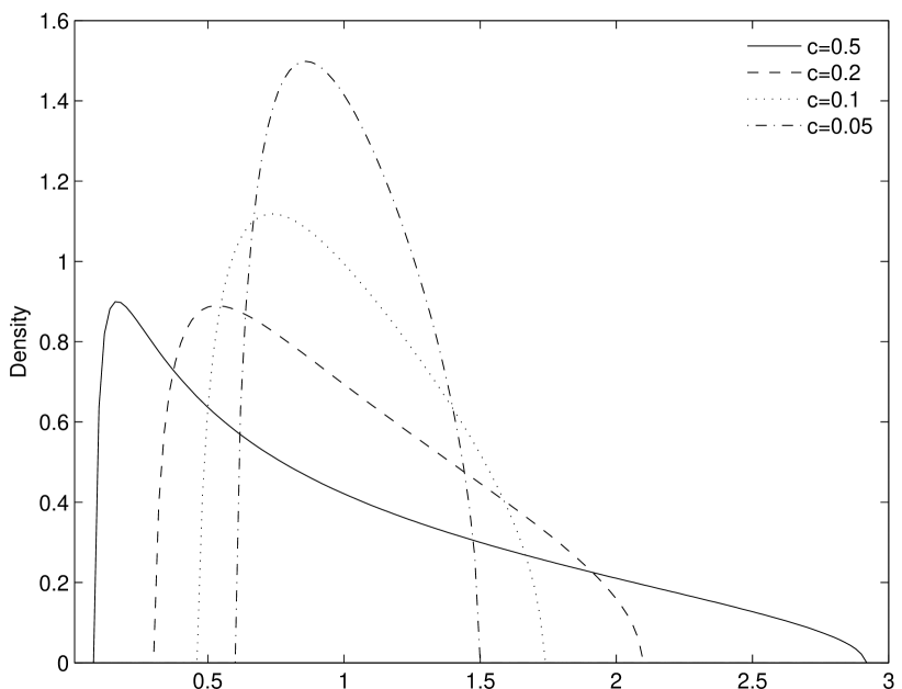
Figure 1: Different Marc̆henko Pastur laws $\mu_{c}$.

It is known that $\mu_{c}$ describes asymptotic eigenvalue distributions of Wishart matrices. Wishart matrices have the form $\frac{1}{N}{\bf R}{\bf R}^{H}$, where ${\bf R}$ is an $n\times N$ random matrix with independent standard Gaussian entries. $\mu_{c}$ appears as limits of such when $\frac{n}{N}\rightarrow c$ when $n\rightarrow\infty$, Note that the Marc̆henko Pastur law can also hold in the limit for non-gaussian entries.

We would like to describe free convolution in terms of the probability densities of the involved measures, since this provides us with the eigenvalue distributions. An important tool in this setting is the Stieltjes transform ([21] page 38). For a probability measure $\mu$, this is the analytic function on ${\BBb C}^{+}=\{z\in C:Imz>0\}$ defined by

$$m_{\mu}(z)=\int\frac{1}{\lambda-z}dF^{\mu}(\lambda),$$ (8)

where $F^{\mu}$ is the cumulative distribution function of $\mu$. All $\mu$ we will consider have support on the positive part of the real line. For such $\mu$, $m_{\mu}$ can be analytically continued to the negative real line, where the values of $m_{\mu}$ are real. If $\mu$ has compact support, we can expand $m_{\mu}(z)$ in a Laurent series, where the coefficient are the moments $\mu_{k}$ of $\mu$:

$$m_{\mu}(z)=-\frac{1}{z}\sum_{k=0}^{\infty}\frac{\mu_{k}}{z^{k}}.$$ (9)

A convenient inversion formula for the Stieltjes transform also exists: We have

$$f^{\mu}(\lambda)=\lim_{\omega\rightarrow 0^{+}}\frac{1}{\pi}Im\left[m_{\mu}(\lambda+j\omega)\right].$$ (10)

III Information plus noise model

In this section we will indicate how the quantities 2) and 3) can be found. The connection between the information plus noise model and free convolution will be made.

III-A Estimation of the sample covariance matrix 2)

In [10], the following result was shown.

Theorem 1

Assume that ${\bf\Gamma}_{n}=\frac{1}{N}{\bf R}_{n}{\bf R}_{n}^{H}$ converge in distribution almost surely to a compactly supported probability measure $\mu_{\Gamma}$. Then we have that ${\bf W}_{n}$ also converge in distribution almost surely to a compactly supported probability measure $\mu_{W}$ uniquely identified by

$$\mu_{W}\begin{picture}(9.0,5.0)\put(2.0,0.0){\framebox(5.0,5.0)[]{$\smallsetminus$}} \end{picture}\mu_{c}=(\mu_{\Gamma}\begin{picture}(9.0,5.0)\put(2.0,0.0){\framebox(5.0,5.0)[]{$\smallsetminus$}} \end{picture}\mu_{c})\boxplus\mu_{\sigma^{2}I}.$$ (11)

Theorem 1 addresses the relationship from 2) to 1), since (11) can be ”deconvolved” to the following form:

$$\mu_{W}=\left((\mu_{\Gamma}\begin{picture}(9.0,5.0)\put(2.0,0.0){\framebox(5.0,5.0)[]{$\smallsetminus$}} \end{picture}\mu_{c})\boxplus\mu_{\sigma^{2}I}\right)\boxtimes\mu_{c}.$$ (12)

It also addresses the relationship from 1) to 2), which is of interest here, through deconvolution in the following form:

$$\mu_{\Gamma}=\left((\mu_{W}\begin{picture}(9.0,5.0)\put(2.0,0.0){\framebox(5.0,5.0)[]{$\smallsetminus$}} \end{picture}\mu_{c})\boxminus\mu_{\sigma^{2}I}\right)\boxtimes\mu_{c}.$$ (13)

III-B Estimation of the covariance matrix 3)

General statistical analysis of observations, also called $G$-analysis [22] [12] is a mathematical theory studying complex systems, where the number of parameters of the considered mathematical model can increase together with the growth of the number of observations of the system. The mathematical models which in some sense approach the system are called $G$-estimators, and the main difficulty in $G$-analysis is to find consistent $G$-estimators. We use $N$ for the number of observations of the system, and $n$ for the number of parameters of the mathematical model. The condition used in $G$-analysis expressing the growth of the number of observations vs. the number of parameters in the mathematical model, is called the $G$-condition. The $G$-condition used throughout this paper is (2).

We restrict our analysis to systems where a number of independent random vector observations are taken, and where the random vectors have identical distributions. If a random vector has length $n$, we will use the notation ${\bf\Theta}_{n}$ to denote the covariance. Girko calls an estimator for the Stieltjes transform of covariance matrices a $G_{2}$-estimator. In chapter 2.1 of [11] he introduces the following expression as candidate for a $G_{2}$-estimator:

$$G_{2,n}(z)=\frac{\hat{\theta}(z)}{z}m_{\mu_{\Gamma_{n}}}(\hat{\theta}(z)),$$ (14)

where the term $m_{\mu_{\Gamma_{n}}}(\hat{\theta}(z))=n^{-1}Tr\left\{{\bf\Gamma}_{n}-\hat{\theta}(z){\bf I}_{n}\right\}^{-1}$. The function $\hat{\theta}(z)$ is the solution to the equation.

$$\hat{\theta}(z)cm_{\mu_{\Gamma_{n}}}(\hat{\theta}(z))-(1-c)+\frac{\hat{\theta}(z)}{z}=0.$$ (15)

Girko claims that a function $G_{2,n}(z)$ satisfying (15) and (14) is a good approximation for the Stieltjes transform of the involved covariance matrices $m_{\mu_{\Theta_{n}}}(z)=\frac{1}{n}Tr\left\{{\bf\Theta}_{n}-z{\bf I}_{n}\right\}^{-1}$. He shows that, for certain values of $z$, $G_{2,n}(z)$ gets close to $m_{\mu_{\Theta_{n}}}(z)$ when $n\rightarrow\infty$.

In [10], the following connection between the $G_{2}$-estimator and multiplicative free convolution is made:

Theorem 2

For the $G_{2}$-estimator given by (14), (15), the following holds for a nonempty open set in ${\BBb C}^{+}$:

$$G_{2,n}(z)=m_{\mu_{\Gamma_{n}}\begin{picture}(9.0,5.0)\put(2.0,0.0){\framebox(5.0,5.0)[]{$\smallsetminus$}} \end{picture}\mu_{c}}$$ (16)

Theorem 2 shows that multiplicative free convolution can be used to estimate the covariance of systems. This addresses the problem of estimating quantity 3). Hence, the estimation of quantity 2) and 3) can be combined, since (13) can be rewritten to

$$\mu_{\Gamma}\begin{picture}(9.0,5.0)\put(2.0,0.0){\framebox(5.0,5.0)[]{$\smallsetminus$}} \end{picture}\mu_{c}=(\mu_{W}\begin{picture}(9.0,5.0)\put(2.0,0.0){\framebox(5.0,5.0)[]{$\smallsetminus$}} \end{picture}\mu_{c})\boxminus\mu_{\sigma^{2}I}.$$ (17)

Therefore, the following procedure needs to take place to estimate quantity 3)

• - perform multiplicative free deconvolution of the measure associated with ${\bf W}_{n}$ and the marchenko pastur law using the $G_{2}$-estimator.

• - perform additive free deconvolution with $\mu_{\sigma^{2}I}$. In other words, perform a shift of the spectrum.

In section V-B, these steps are performed in the setting of channel correlation estimation. The combinatorial implementation of free deconvolution from section IV-A1 is used to compute the $G_{2}$-estimator.

We plot in figure 2 histograms of eigenvalues for various sample covariance matrices when the rank is $K=8$. As one can see, if the number of sensors ($N$) are chosen much larger than the number of signals $K$, the eigenvalues corresponding to the signals only make up a small portion of the entire set of eigenvalues. If one has information on the number of impinging signals, it can therefore be wise to choose the appropriate number of sensors.

(a) $N=64$

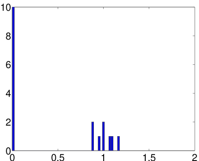
(b) $N=512$

Figure 2: Histograms of eigenvalues of sample covariance matrices. The covariance matrix has rank $K=8$. We choose different number of sensors $N$, and choose $c=0.5$ (so that $L=2N$ observations are taken).

In this paper, the difference between a probability measure, $\mu$, and an estimate of it, $\nu$, will be measured in terms of the Mean Square Error of the moments (MSE). If the moments of $\int x^{k}d\mu(x)$, $\int x^{k}d\nu(x)$ are denoted by $\mu_{k}$, $\nu_{k}$, respectively, the MSE is defined by

$$\sum_{k\leq n}|\mu_{k}-\nu_{k}|^{2}$$ (18)

for some number $n$. In our estimation problems, the measure $\nu$ we test which gives the minimum MSE (MMSE) will be chosen.

The measure $\mu$ can either be given explicitly in terms of the distribution of matrices $R_{n}$ (for which the measure is discrete and the moments are given by $\nu_{k}=tr_{n}(R_{n}^{k})$), or random matrices, or it can be given in terms of just the moments. In a free probability setting, giving just the moments is often convenient, since free convolution can be viewed as operating on the moments. Since the $G_{2}$-estimator uses free deconvolution, it will be subject to a Mean Square Error of moments analysis. We will compute the MSE for different number of moments, depending on the availability of the moments.

In figure 3, a covariance matrix with density $\frac{1}{2}\delta_{0}+\frac{1}{2}\delta_{1}$ has been estimated with the the $G_{2}$-estimator. Sample covariance matrices of various sizes are formed, and method A in section IV-A1 was used for the free deconvolution in the $G_{2}$-estimator. Finally, MSE of the first $4$ and $8$ moments were computed. It is seen that the MSE decreases with the matrix sizes, which confirms the accuracy of the $G_{2}$-estimator. Also, the MSE is much higher when more moments are included. This is as expected, when we compare known exact expressions for moments of Gaussian random matrices [23], with the limits these converge to.

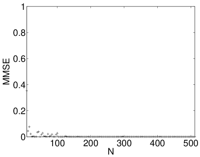
(a) 4 moments

(b) 8 moments

Figure 3: MMSE of the first moments of the covariance matrices, and the first moments of the $G_{2}$ estimator of the sample covariance matrices. The covariance matrices all have distribution $\frac{1}{2}\delta_{0}+\frac{1}{2}\delta_{1}$. Different matrix sizes $N$ are tried. The value $c=0.5$ is used.

Since the MSE is typically higher in the higher moments, we will in the simulations in this paper minimize a weighted MSE:

$$\sum_{k}w_{k}|\mu_{k}-\nu_{k}|^{2},$$ (19)

instead of the MSE in (18). Higher moments should have smaller weights $w_{k}$, since errors in random matrix models are typically larger in the higher moments. There may not be optimal weights which work for all cases. For the cases in this paper, the weights are $w_{2k}=\left(\stackrel{{\scriptstyle 2k}}{{k}}\right)$ and $w_{2k+1}=0$, whick coincide with the Catalan numbers $C_{k}$. These weights are motivated from formulas for moments of Gaussian random matrices in the way explained below, and are used in this paper since the models we consider often involve Gaussian matrices.

Moment $2k$ of a standard selfadjoint Gaussian matrix $X_{n}$ of size $n\times n$ satisfies [14] [24]

$$\lim_{n\rightarrow\infty}\tau_{n}({\bf X}_{n}^{2k})=C_{k}.$$

Also, exact formulas for $\tau_{n}({\bf X}_{n}^{2k})$ (4.1.19 in [14]) exist, where the proof uses combinatorics and noncrossing partitions (see section IV-A1), with emphasis on the quantity $C_{k}$ being the number of noncrossing partitions of $\{1,...,2k\}$ where all blocks have cardinality two. From the exact formula for the moment of $\tau_{n}({\bf X}_{n}^{2k})$, one can also see the difference between the limit as $n\rightarrow\infty$. This difference is approximately $n^{-1}\times card(S)$, where $S$ is another set of partitions. Although this set of partitions is not the same as the noncrossing partitions, it can in some sense be thought of as ”partitions where limited crossings may be allowed”. The choice of $C_{k}$ as weight is merely motivated from the belief that $S$ possibly has similar properties as the noncrossing partitions, and that possibly the cardinality has a similar expression.

In summary, figure 3 shows that for large matrices, the $G_{2}$-estimator gets close to the actual covariance matrices although several sources can give contribution to errors:

1. The sample covariance matrix itself is estimated,

2. the estimator itself contributes to the error,

3. the implementation of free deconvolution also contributes to the error.

IV Computation of free convolution

One of the challenges in free probability theory is the practical computation of free convolution. Usual results exhibit asymptotic convergence of product and sum of measures, but do not explicitly provide a framework for computing the result. In this section, given two compactly supported probability measures, we will sketch how their free (de)convolved counterparts can be computed. In the cases we are interested (signal impaired with noise), the Marc̆henko Pastur law $\mu_{c}$ will be one of the operand measures, while the other will be a discrete measure, i.e. with density

$$f^{\mu}(x)=\sum_{i=1}^{n}p_{i}\delta_{\lambda_{i}}(x),$$ (20)

where $p_{i}$ is the mass at $\lambda_{i}$, and $\sum_{i}p_{i}=1$. All $\lambda_{i}\geq 0$, since only measures with support on the positive real line are considered ($n\times n$ sample covariance matrices have such eigenvalue distributions). This would be the distribution we observe in a practical scenario: Since a finite number of samples are taken, we only observe a discrete estimate of the sample covariance matrix.

The Stieltjes transform $m_{\mu_{c}\begin{picture}(9.0,5.0)\put(2.0,0.0){\framebox(5.0,5.0)[]{$\smallsetminus$}} \end{picture}\mu}$ can be found exactly for $z$ on the negative real line by solving function equations [10], but one has to perform analytical continuation to the upper half of the complex plane prior to using the Stieltjes inversion formula. Indeed, note that since the power series (9) is only known to converge for $z$ outside a disk with radius equal to the spectral radius, partial sums of (9) can not necessarily be used to approach the limit in (10). However, one can show that values of $m_{\mu}(z)$ for $z$ on the negative real line can be approximated by analytically continuing partial sums of (9).

When $\mu$ is discrete, one can show that solving the function equations boils down to finding the roots of real polynomials (see section IV-B), which then must be analytically continued. We will sketch a particular case where this can be performed exactly. We will also sketch two other methods for computing free convolution numerically. One method uses a combinatorial description, which easily admits an efficient recursive implementation. The other method is based on results on asymptotic freeness of large random matrices.

IV-A Numerical Methods

IV-A1 Method A: Combinatorial computation of free convolution

The concept we need for computation of free convolution presented in this section is that of noncrossing partitions [24]:

Definition 4

A partition $\pi$ is called noncrossing if whenever we have $i<j<k<l$ with $i\sim k$, $j\sim l$ ($\sim$ meaning belonging to the same block), we also have $i\sim j\sim k\sim l$ (i.e. $i,j,k,l$ are all in the same block). The set of noncrossing partitions of $\{1,,,.,n\}$ is denoted $NC(n)$.

We will write $\pi=\{B_{1},...,B_{r}\}$ for the blocks of a partition. $|B_{i}|$ will mean the cardinality of the block $B_{i}$.

Additive free convolution.

A convenient way of implementing additive free convolution comes through the moment-cumulant formula, which expresses a relationship between the moments of the measure and the associated $R$-transform ([21] page 48). The $R$-transform has domain of definition ${\BBb C}^{+}$ and can be defined in terms of the Stieltjes transform as

$${\cal R}_{\mu}(z)=m_{\mu}^{-1}(-z)-\frac{1}{z}.$$ (21)

The importance of the $R$-transform comes from the additivity property in additive free convolution,

$${\cal R}_{\mu_{1}\boxplus\mu_{2}}(z)={\cal R}_{\mu_{1}}(z)+{\cal R}_{\mu_{2}}(z).$$ (22)

Slightly different versions of the $R$-transform are encountered in the literature. The definition (21) is from [21]. In connection with free combinatorics, another definition is used, namely $R_{\mu}(z)=z{\cal R}_{\mu}(z)$. Write $R_{\mu}(z)=\sum_{n}\alpha_{n}z^{n}$. The coefficients $\alpha_{n}$ are called cumulants. The moment-cumulant formula says that

$$\mu_{n}=\sum_{\pi=\{B_{1},\cdots,B_{k}\}\in NC(n)}\prod_{i=1}^{k}\alpha_{|B_{i}|}.$$ (23)

From (23) it follows that the first $n$ cumulants can be computed from the first $n$ moments, and vice versa. Noncrossing partitions have a structure which makes them easy to iterate over in an implementation. One can show that (23) can be rewritten to the following form suitable for implementation:

$$\mu_{n}=\sum_{k\leq n}\alpha_{k}coef_{n-k}\left((1+\mu_{1}z+\mu_{2}z^{2}+\cdots)^{k}\right).$$ (24)

Here $coef_{k}$ means the coefficient of $z^{k}$. Computing the coefficients of $(1+\mu_{1}z+\mu_{2}z^{2}+\cdots)^{k}$ can be implemented in terms of a $k$-fold discrete (classical) convolution, so that the connection between free and classical convolution can be seen both in terms of concept and implementation. (24) can be implemented in such a way that the $\mu_{n}$ are calculated from $\alpha_{n}$, or, the other way around, the $\alpha_{n}$ are calculated from the $\mu_{n}$. When computing higher moments, (24) is quite time-consuming, since many (classical) convolutions of long sequences have to be performed. A recursive implementation of (24) was made for this paper [25], and is briefly described in appendix A. The paper [26] goes through implementation issues of free convolution in more detail.

Additive free convolution in terms of moments of the involved measures can therefore beimplemented through the following steps: Evaluate cumulants using (24) for the two measures, add these, and finally evaluate moments using (24) also.

Multiplicative free convolution.

The combinatorial transform we need for multiplicative free convolution is that of boxed convolution [24] (denoted by $\framebox[7.0pt]{$\star$}$), which can be thought of as a convolution operation on formal power series. The definition uses noncrossing partitions and will not be stated here. One power series will be of particular importance to us. The $Zeta$-series is intimately connected to $\mu_{1}$ in that it appears as it’s $R$-transform. It is defined by

$$Zeta(z)=\sum_{i}z^{i}.$$

$Zeta(z)$ has an inverse under boxed convolution,

$$Moeb(z)=\sum_{n=1}^{\infty}(-1)^{n-1}C_{n-1}z^{n},$$

also called the Möbius series. Here $(C_{n})_{n=1}^{\infty}$ is the sequence of Catalan numbers (which are known to be related to the even moments of Wigner matrices). Define the moment series of a measure $\mu$ by

$$M(\mu)(z)=\sum_{k=1}^{\infty}\mu_{k}z^{k}=-\frac{1}{z}m_{\mu}(\frac{1}{z})-1.$$

One can show that (23) is equivalent to $M(\mu)=R(\mu)\framebox[7.0pt]{$\star$}Zeta$. One can in fact show that boxed convolution on power series is the combinatorial perspective of multiplicative free convolution on measures. Also,

1. boxed convolution with the power series $c^{n-1}Zeta$ represents convolution with the measure $\mu_{c}$,

2. boxed convolution with the power series $c^{n-1}Moeb$ represents deconvolution with the measure $\mu_{c}$.

This is formalized as

$$M_{\mu\boxtimes\mu_{c}}=M_{\mu}\framebox[7.0pt]{$\star$}(c^{n-1}Zeta),$$

and can also be rewritten to

$$cM_{\mu\boxtimes\mu_{c}}=Zeta\framebox[7.0pt]{$\star$}(cM_{\mu}),$$ (25)

It can be shown that this is nothing but the moment-cumulant formula, with cumulants replaced by the coefficients of $cM_{\mu}$, and moments replaced by the coefficients $cM_{\mu\boxtimes\mu_{c}}$. Therefore, the same computational procedure can be used for passing between moments and cumulants, as for passing between the moments series of $\mu\boxtimes\mu_{c}$ and that of $\mu$, the only difference being the additional scaling of the moments by $c$:

1. multiply all input moments by $c$ prior to execution of (24),

2. divide all output moments by $c$ after execution of (24).

The situation for other compactly supported measures than $\mu_{c}$ follows the same lines, but with $c^{n-1}Zeta$ and $c^{n-1}Moeb$ replaced with other power series. Convolution and deconvolution with other measures than $\mu_{c}$ may be harder to implement, due to the particularly simple structure of the $Zeta$ series.

In addition to computing (24) and performing step 1) and 2) above, we need first to obtain the moments of $\mu$ in some way. For $\mu$ as in (20) the moments can be calculated by incrementally computing the numbers $(\lambda_{1}^{m},...,\lambda_{n}^{m})$, adding these together and normalizing. At the end, we may also need to retrieve the probability density from the computed moments. If a density corresponds to the eigenvalue distribution of some matrix, the Newton-Girard Formulas [27] can be used to retrieve the eigenvalues from the moments. These formulas state a relationship between the elementary symmetric polynomials

$$\Pi_{j}(\lambda_{1},...,\lambda_{n})=\sum_{i_{1}<\cdots<i_{j}\leq n}\lambda_{i_{1}}\cdots\lambda_{i_{j}},$$ (26)

and the sums of the powers of their variables

$$S_{p}(\lambda_{1},...,\lambda_{n})=\sum_{1\leq i\leq n}\lambda_{i}^{p},$$ (27)

through the recurrence relation

$$\begin{array}[]{ll}&(-1)^{m}m\Pi_{m}(\lambda_{1},...,\lambda_{n})\\ +&\sum_{k=1}^{m}(-1)^{k+m}S_{k}(\lambda_{1},...,\lambda_{n})\Pi_{m-k}(\lambda_{1},...,\lambda_{n})=0.\end{array}$$ (28)

If $S_{p}(\lambda_{1},...,\lambda_{n})$ are known for $1\leq p\leq n$, (28) can be used repeatedly to compute $\Pi_{m}(\lambda_{1},...,\lambda_{n})$, $1\leq m\leq n$.

Coefficient $n-k$ in the characteristic polynomial

$$(\lambda-\lambda_{1})\cdots(\lambda-\lambda_{n})$$

is $(-1)^{k}\Pi_{k}(\lambda_{1},...,\lambda_{n})$, and these can be computed from $S_{k}(\lambda_{1},...,\lambda_{n})$ using (28). Since $S_{k}(\lambda_{1},...,\lambda_{n})=nm_{k}$ (with $m_{k}$ being the kth moment), the entire characteristic polynomial can be computed from the moments. Hence, the eigenvalues can be found also.

In general, the density can not be written as the eigenvalue distribution of a matrix, but the sketched procedure can still provide us with an estimate based on the moments. Intuitively, the approximation should work better when more moments are involved. The simulations in this paper use the sketched procedure only for a low number of moments, since mostly discrete measures with few atoms are estimated. We have thus also avoided issues for solving higher degree characteristic equations with high precision.

IV-A2 Method B: Computation of free convolution based on asymptotic freeness results

As mentioned, the Marc̆henko Pastur law can be approximated by random matrices of the form ${\bf\Gamma}_{n}=\frac{1}{N}{\bf R}_{n}{\bf R}_{n}^{H}$, where ${\bf R}_{n}$ is $n\times N$ with i.i.d. standard Gaussian entries. It is also known that the product of such a ${\bf\Gamma}_{n}$ with a (deterministic) matrix with eigenvalue distribution $\mu$ has an eigenvalue distribution which approximates that of $\mu_{c}\boxtimes\mu$. This is formulated in free probability as a result on asymptotic freeness of certain random matrices with deterministic matrices [14]. Therefore, one can approximate multiplicative free convolution by taking a sample from a random matrix ${\bf\Gamma}_{n}$, multiply it with a deterministic diagonal matrix with eigenvalue distribution $\mu$, and calculating the eigenvalue distribution of this product. The deterministic matrix need not be diagonal. Additive free convolution can be estimated in the same way by adding ${\bf\Gamma}_{n}$ and the deterministic matrix instead of multiplying them.

In figure 4, method B is demonstrated for various matrix sizes to obtain approximations of $\left(\frac{1}{2}\delta_{0}+\frac{1}{2}\delta_{1}\right)\boxtimes\mu_{c}$ for $c=0.5$. The moments of the approximations are compared with the exact moments, which are obtained with method A. The Mean Square Error of the moments is used to measure the difference. As in figure 3, it is seen that the MSE decreases with the matrix sizes, and that the MSE is much higher when more moments are included.

(a) 4 moments

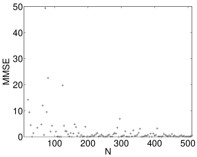
(b) 8 moments

Figure 4: MMSE of the first moments of $\left(\frac{1}{2}\delta_{0}+\frac{1}{2}\delta_{1}\right)\boxtimes\mu_{c}$, and the same moments computed approximately with method B using different matrix sizes $N$. The value $c=0.5$ is used.

Another interesting phenomenon occurs when we let $c$ go to $0$, demonstrated in figure 5 for the measure $\mu$ with

$$f^{\mu}(x)=\frac{1}{3}\delta_{1}(x)+\frac{1}{3}\delta_{3}(x)+\frac{1}{3}\delta_{4}(x).$$ (29)

It is seen that for small $c$, the support of $\mu\boxtimes\mu_{c}$ seems to split into disjoint components centered at the dirac locations. This is compatible with results from [28]. There it is just noted that, for a given type of systems, the support splits into TWO different components, and the relative mass between these components is used to estimate the numbers of signals present in the systems they consider.

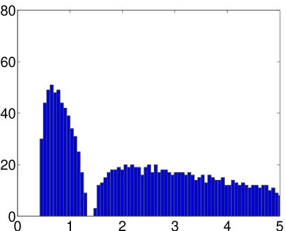
(a) $c=0.2$. $L=7680$ observations

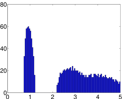
(b) $c=0.05$. $L=30720$ observations

Figure 5: Approximated densities of $\left(\frac{1}{3}\delta_{1}(x)+\frac{1}{3}\delta_{3}(x)+\frac{1}{3}\delta_{4}(x)\right)\boxtimes\mu_{c}$ with method B for various values of $c$

In figure 5, a matrix of dimension $N\times N$ with $N=1536$ and eigenvalue distribution $\mu$ is taken. This matrix is multiplied with a Wishart matrix $\frac{1}{L}{\bf X}{\bf X}^{H}$, where ${\bf X}$ has dimension $N\times L$ with $\frac{N}{L}=c$ with decreasing values of $c$. It is seen that the dirac at $1$ is split from the rest of the support in both plots, with the split more visible for the lower value of $c$. The splitting of the two other diracs from each other it not very visible for these values of $c$. Also, the peaks in the density of $\mu\boxtimes\mu_{c}$ occur slightly to the left of the dirac points, which is as expected from the comments succeeding theorem 3.

A partial explanation for the fact that $\mu\boxtimes\mu_{c}$ in some sense converges to $\mu$ when $c\rightarrow 0$ is given by combining the following facts:

• The sample covariance matrix converges to the true covariance matrix when the number of observations tend to $\infty$ (i.e. $c\rightarrow 0$).

• The $G_{2}$-estimator for the covariance matrices is given by multiplicative free deconvolution with $\mu_{c}$.

In summary, the differences between method A and B are the following:

1. Method B needs to compute the full eigenvalue distribution of the operand matrices. Method A works entirely on the moments.

2. With method B, the results are only approximate. If the eigenvalues are needed also, method A needs to perform computationally expensive tasks in approximating eigenvalues from moments, for instance as described in section IV-A1.

3. Method B is computationally more expensive, in that computations with large matrices are needed in order to obtain accurate results. Method A is scalable in the sense that performance scales with the number of moments computed. The lower moments are the same regardless on how many higher moments are computed.

The two methods should really be used together: While method A easily can get exact moments, method B can tell us the accuracy of random matrix approximations by comparison with these exact moments.

The simulations in this paper will use method A, since deconvolution is a primary component, and since we in many cases can get the results with an MSE of moments analysis. Deconvolution with method B should correspond to multiplication with the inverse of a Wishart matrix, but initial tests do not suggest that this strategy works very well when predicting the deconvolved eigenvalues.

The way method A and method B have been described here, they have in common that they only work for free convolution and deconvolution with Marc̆henko Pastur laws. Method A worked since (24) held for such laws, while method B worked since these laws have a convenient asymptotic random matrix model in terms of Gaussian random matrices.

IV-B Non-numerical methods: Exact calculations of multiplicative free convolution

Computation of free convolution in general has to be performed numerically, for instance through the methods in section IV-A1 and IV-A2. In some cases, the computation can be performed exactly, i.e. the density of the (de)convolutions can be found exactly. Consider the specific case of (20) where

$$f^{\mu}(x)=(1-p)\delta_{0}(x)+p\delta_{\lambda}(x),$$ (30)

where $p<1$, $\lambda>0$. Such measures were considered in [13], where deconvolution was implemented by finding a pair $(p,\lambda)$ minimizing the difference between the moments of $\mu\boxtimes\mu_{c}$, and the moments of observed sample covariance matrices. Exact expressions for the density of $\mu\boxtimes\mu_{c}$ were not used, all calculations were performed in terms of moments.

(30) contains one dirac (i.e. $p=1$) as a special case. It is clear that multiplicative free convolution with $\delta_{\lambda}$ has an exact expression, since we simply multiply the spectrum with $\lambda$ (the spectrum is scaled). As it turns out, all $\mu$ of the form (30) give an exact expression for $\mu\boxtimes\mu_{c}$. In appendix B, the following is shown:

Theorem 3

The density of $\mu\boxtimes\mu_{c}$ is $0$ outside the interval

$$I_{\lambda,c,p}=\left[\lambda(1+cp)-2\lambda\sqrt{cp},\lambda(1+cp)+2\lambda\sqrt{cp}\right],$$ (31)

while the density on $I_{\lambda,c,p}$ is given by

$$f^{\mu\boxtimes\mu_{c}}(x)=\frac{\sqrt{K_{1}(x)K_{2}(x)}}{2c\lambda x\pi},$$ (32)

where

$$\begin{array}[]{lll}K_{1}(x)&=&x-\lambda(1+cp)+2\lambda\sqrt{cp}\\ K_{2}(x)&=&\lambda(1+cp)+2\lambda\sqrt{cp}-x.\end{array}$$

The density has a unique maximum at $x=\lambda\frac{(1-cp)^{2}}{1+cp}$, with value $\frac{\sqrt{cp}}{c\pi\lambda(1-cp)}$.

The importance of theorem 3 is apparent: The mass of $\mu\boxtimes\mu_{c}$ is seen to be centered on $\lambda(1+cp)$, with support width of $4\lambda\sqrt{cp}$. If we let $c$ go to zero, the center of mass approaches $\lambda$ and the support width approaches zero. We note that the center of the support of $\mu\boxtimes\mu_{c}$ is slighly perturbed to the right of $\lambda$, while the density maximum occurs slightly to the left of $\lambda$. It is easily checked that the support width and the maximum density uniquely identifies a pair $(p,\lambda)$. This means that, if we have an estimate of the density of $\mu\boxtimes\mu_{c}$ (for instance in the form of a realization of a sample covariance matrix) for a measure $\mu$ of the form (30), the maximum density and the support width give us a good candidate for the $(p,\lambda)$ defining $\mu$. Figure 6 shows densities of some realizations of $\mu\boxtimes\mu_{c}$ for $p=\frac{1}{2}$ and $\lambda=1$, together with corresponding realizations of covariances matrices. Values $c=0.25$ and $c=0.5$ were used, with $L=1024$ and $L=2048$ observations respectively. Covariance matrices of size $512\times 512$ were used.

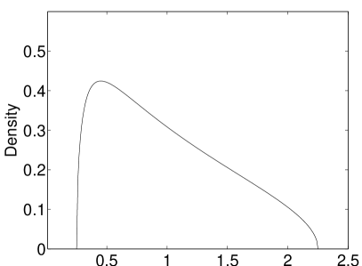
(a) $c=0.5$

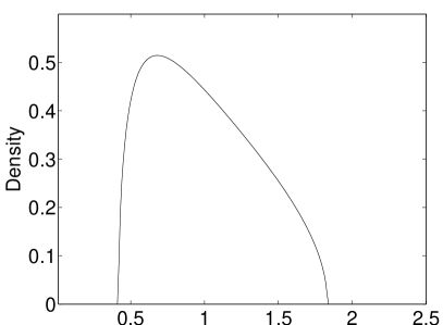
(b) $c=0.25$

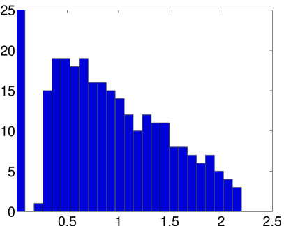
(c) $c=0.5$. $L=1024$ observations

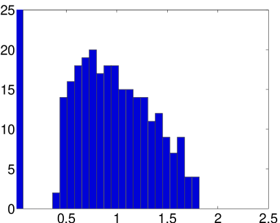
(d) $c=0.25$. $L=2048$ observations

Figure 6: Densities of $\left(\frac{1}{2}\delta_{0}+\frac{1}{2}\delta_{1}\right)\boxtimes\mu_{c}$ (upper row), and corresponding histogram of eigenvalues for the sample covariance matrices for different number of observations (lower row)

A similar result to theorem 3 characterizing $\mu\begin{picture}(9.0,5.0)\put(2.0,0.0){\framebox(5.0,5.0)[]{$\smallsetminus$}} \end{picture}\mu_{c}$ is proved in appendix C:

Theorem 4

The density of $\mu\begin{picture}(9.0,5.0)\put(2.0,0.0){\framebox(5.0,5.0)[]{$\smallsetminus$}} \end{picture}\mu_{c}$ is $0$ outside the interval

$$\begin{array}[]{lll}J_{\lambda,c,p}&=&[\lambda(1-2cp)-2\lambda\sqrt{cp(1-cp)}\\ &&\lambda(1-2cp)+2\lambda\sqrt{cp(1-cp)}],\end{array}$$ (33)

while the density on $J_{\lambda,c,p}$ is given by

$$f^{\mu\begin{picture}(9.0,5.0)\put(2.0,0.0){\framebox(5.0,5.0)[]{$\smallsetminus$}} \end{picture}\mu_{c}}(x)=\frac{\sqrt{L_{1}(x)L_{2}(x)}}{2cx^{2}},$$ (34)

where

$$\begin{array}[]{lll}L_{1}(x)&=&x-\lambda(1-2cp)+2\lambda\sqrt{cp(1-cp)}\\ L_{2}(x)&=&\lambda(1-2cp)+2\lambda\sqrt{cp(1-cp)}-x.\end{array}$$

The support in this case is centered on $\lambda(1-2cp)$, which is slightly to the left of $\lambda$, contrary to the case of convolution. The support width is $4\lambda\sqrt{cp(1-cp)}$. Also in this case it is easily seen that the support narrows and gets centered on $\lambda$, as $c$ goes to $0$. The densities in (32) and (34) are seen to resemble the density of $\mu_{c}$ in (7). One difference is that $\mu_{c}$ is centered on $1$, while the densities in (32) and (34) need not be.

The proofs of theorem 3 and 4 build on an analytical machinery for computing free convolution, where several transforms play a role. Besides the Stieltjes transform $m_{\nu}(z)$, one has the $\eta$-transform, defined for real $z\geq 0$

$$\eta_{\nu}(z)=\int_{-\infty}^{\infty}\frac{1}{1+z\lambda}dF^{\nu}(\lambda).$$

It is easy to verify that $m_{\nu}$ can be analytically continued to the negative part of the real line, and that

$$\eta_{\nu}(z)=\frac{m_{\nu}\left(-\frac{1}{z}\right)}{z}$$ (35)

for $z\geq 0$. The $\eta$-transform has some nice properties, it is for instance strictly monotone decreasing, so that it has an inverse. In [10] it was shown that

$$\eta_{\mu\boxtimes\mu_{c}}^{-1}(z)=\frac{\eta_{\mu}^{-1}(z)}{1-c+cz}.$$ (36)

The proof of this involved some more transforms, like the $S$-transform, and the actual value of these transforms for $\mu_{c}$. The following forms will be more useful to us than (36), and can be deduced easily from it:

$$\eta_{\mu}\left(z(1-c+c\eta_{\mu\boxtimes\mu_{c}}(z))\right)=\eta_{\mu\boxtimes\mu_{c}}(z)$$ (37)

and

$$\eta_{\mu}\left(\frac{z}{1-c+c\eta_{\mu\begin{picture}(9.0,5.0)\put(2.0,0.0){\framebox(5.0,5.0)[]{$\smallsetminus$}} \end{picture}\mu_{c}}(z)}\right)=\eta_{\mu\begin{picture}(9.0,5.0)\put(2.0,0.0){\framebox(5.0,5.0)[]{$\smallsetminus$}} \end{picture}\mu_{c}}(z).$$ (38)

$\eta_{\mu}(z)$ for $\mu$ as in (30) is easily calculated:

$$\eta_{\mu}(z)=1-p+\frac{p}{1+z\lambda}.$$ (39)

$\mu\boxtimes\mu_{c}$ with unconnected support components centered at the dirac locations of $\mu$ may very well happen for discrete measures with more than two atoms also, but we do not address this question here. The more general case, even when there are two dirac’s away from $0$, does not admit a closed-form solution, since higher degree equations in general can not be solved using algebraic methods. However, one can still solve those equations numerically: For $\mu$ on the more general form (20), the $\eta$-transform is

$$\eta_{\mu}(z)=\sum_{i=1}^{n}\frac{p_{i}}{1+z\lambda_{i}}.$$

Putting this into (37), we see that we can solve

$$\sum_{i=1}^{n}\frac{p_{i}}{1+z\lambda_{i}\left(1-c+c\eta_{\mu\boxtimes\mu_{c}}(z)\right)}=\eta_{\mu\boxtimes\mu_{c}}(z)$$

to find $\eta_{\mu\boxtimes\mu_{c}}(z)$. Collecting terms, we see that this is a higher order equation in $\eta_{\mu\boxtimes\mu_{c}}(z)$. $m_{\mu}(z)$ and hence the density of $\mu$ can then be found from (35).

V Applications to signal processing

In this section, we provide several applications of free deconvolution and show how the framework can be used in this paper.

V-A Estimation of power and the number of users

In communication applications, one needs to determine the number of users in a cell in a CDMA type network as well the power with which they are received (linked to the path loss). Denoting by $n$ the spreading length, the received vector at the base station in an uplink CDMA system is given by:

$${\bf y}_{i}={\bf W}{\bf P}^{\frac{1}{2}}{\bf s}_{i}+{\bf b}_{i}$$ (40)

where ${\bf y}_{i}$, ${\bf W}$, ${\bf P}$, ${\bf s}_{i}$ and ${\bf b}_{i}$ are respectively the $n\times 1$ received vector, the $n\times N$ spreading matrix with i.i.d zero mean, $\frac{1}{n}$ variance entries, the $N\times N$ diagonal power matrix, the $N\times 1$ i.i.d gaussian unit variance modulation signals and the $n\times 1$ additive white zero mean Gaussian noise.

Usual methods determine the power of the users by finding the eigenvalues of covariance matrix of ${\bf y}_{i}$ when the signatures (matrix ${\bf W}$) and the noise variance are known.

$${\bf\Theta}={\mathbb{E}}\left({\bf y}_{i}{\bf y}_{i}^{H}\right)={\bf W}{\bf P}{\bf W}^{H}+\sigma^{2}{\bf I}$$ (41)

However, in practice, one has only access to an estimate of the covariance matrix and does not know the signatures of the users. One can solely assume the noise variance known. In fact, usual methods compute the sample covariance matrix (based on $L$ samples) given by:

$$\hat{\bf\Theta}=\frac{1}{L}\sum_{i=1}^{L}{\bf y}_{i}{\bf y}_{i}^{H}$$ (42)

and determine the number of users (and not the powers) in the cell by the non zero-eigenvalues (or up to an ad-hoc threshold for the noise variance) of:

$$\hat{\bf\Theta}-\sigma^{2}{\bf I}$$ (43)

This method, referred here as classical method, is quite inadequate when $L$ is in the same range as $n$. Moreover, it does not provide a method for the estimation of the power of the users.

The free deconvolution framework introduced in this paper is well suited for this case and enables to determine the power of the users without knowing their specific code structure. Indeed, the sample covariance matrix is related to the true covariance matrix ${\bf\Theta}={\mathbb{E}}\left({\bf y}_{i}{\bf y}_{i}^{H}\right)$ by:

$$\hat{\bf\Theta}={\bf\Theta}^{\frac{1}{2}}{\bf X}{\bf X}^{H}{\bf{\bf\Theta}^{\frac{1}{2}}}$$ (44)

with

$${\bf\Theta}={\bf W}{\bf P}{\bf W}^{H}+\sigma^{2}{\bf I}$$ (45)

and ${\bf X}$ is a $n\times L$ i.i.d Gaussian zero mean matrix.

Combining (44), (45), with the fact that ${\bf W}^{H}{\bf W}$, $\frac{1}{L}{\bf X}{\bf X}^{H}$ are Wishart matrices with distributions approaching $\mu_{\frac{N}{n}}$, $\mu_{\frac{n}{L}}$ respectively, and using that

$$\mu_{{\bf W}{\bf P}{\bf W}^{H}}=\frac{N}{n}\mu_{{\bf W}^{H}{\bf WP}}+\left(1-\frac{N}{n}\right)\delta_{0},$$

we get due to asymptotic freeness the equation

$$\left(\left(\frac{N}{n}(\mu_{\frac{N}{n}}\boxtimes\mu_{{\bf P}})+\left(1-\frac{N}{n}\right)\delta_{0}\right)\boxplus\mu_{\sigma^{2}I}\right)\boxtimes\mu_{\frac{n}{L}}=\mu_{\bf\hat{R}}$$ (46)

If one knows the noise variance, one can use this equation in simulations in two ways:

1. Through additive and multiplicative free deconvolution, use (46) where the power distribution of the users (and de facto the number of users) is expressed in terms of the sample covariance matrices.

2. Determine the numbers of users $N$ through a best-match procedure: Try all values of $N$ with $1\leq N\leq n$, and choose the $N$ which gives a best match between the left and right hand side in (46).

To solve (46), method A was used to compute the moments. In order to solve (13), we also need to compute additive free deconvolution with a scalar. This was addressed in section IV-A1, but can also be computed in a simpler way, since

$$\phi((a-\sigma^{2}I)^{j})=\sum_{k=0}^{j}(-1)^{k}\left(\stackrel{{\scriptstyle j}}{{k}}\right)\sigma^{2k}\phi(a^{j-k}).$$

In (46) we also scale a measure with $\frac{N}{n}$, and add an atom at $0$. Both of these cases are easily implemented.

In the following simulations, a spreading length of $n=256$ and noise variance $\sigma^{2}=0.1$ have been used.

V-A1 Estimation of power

We use a $36\times 36$ ($N=36$) diagonal matrix as our power matrix ${\bf P}$, and use three sets of values, at 0.5, 1 and 1.5 with equal probability, so that

$$\mu_{\bf P}=\frac{1}{3}\delta_{0.5}+\frac{1}{3}\delta_{1}+\frac{1}{3}\delta_{1.5}.$$ (47)

There are no existing methods for estimating such a $\mu_{\bf P}$ from the sample covariance matrices: to our knowledge, existing methods estimate the power with non-zero eigenvalues of the sample covariance matrix up to $\sigma^{2}$. In our case, the powers are all above $\sigma^{2}$.

(a) $L=256$

(b) $L=512$

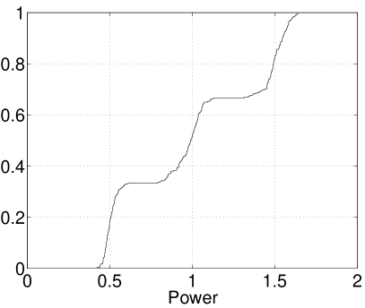
(c) $L=1024$

(d) $L=2048$

Figure 7: CDF of powers estimated from multiplicative free deconvolution from sample covariance matrices with different number of observations.

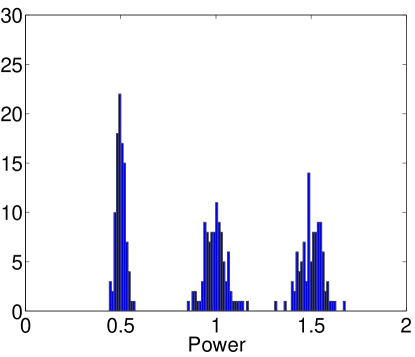
Figure 8: Distribution of the powers estimated from multiplicative free deconvolution from sample covariance matrices with $L=2048$.

In figure 7, the CDF of $\mu_{\bf P}$ was estimated by solving (46), using method A with three moments. The resulting moments from method A were used to compute estimates of the eigenvalues through the Newton-Girard formula, and the CDF was computed by averaging these eigenvalues for 100 runs for each number of observations. An alternative strategy would be to use higher moments, and less runs for each observation. As one can see, when L increases, we get a CDF closer to that of (47). The best result is obtained for $L=2048$. The corresponding histogram of the eigenvalues in this case is shown in figure 8.

V-A2 Estimation of the number of users

We use a $36\times 36$ ($N=36$) diagonal matrix as our power matrix ${\bf P}$ with $\mu_{\bf P}=\delta_{1}$. In this case, a common method that try to find just the rank exists. This method determines the number of eigenvalues greater than $\sigma^{2}$. Some threshold is used in this process. We will set the threshold at $1.5\sigma^{2}$, so that only eigenvalues larger that $1.5\sigma^{2}$ are counted. There are no general known rules for where the threshold should be set, so some guessing is inherent in this method. Also, choosing a wrong threshold can lead to a need for a very high number of observations for the method to be precise.

We will compare this classical method with a free convolution method for estimating the rank, following the procedure sketched in step 2). The method is tested with varying number of observations, from $L=1$ to $L=4000$, and the $N$ which gives the best match with the moments of the SCM in (46) is chosen. Only the four first moments are considered.

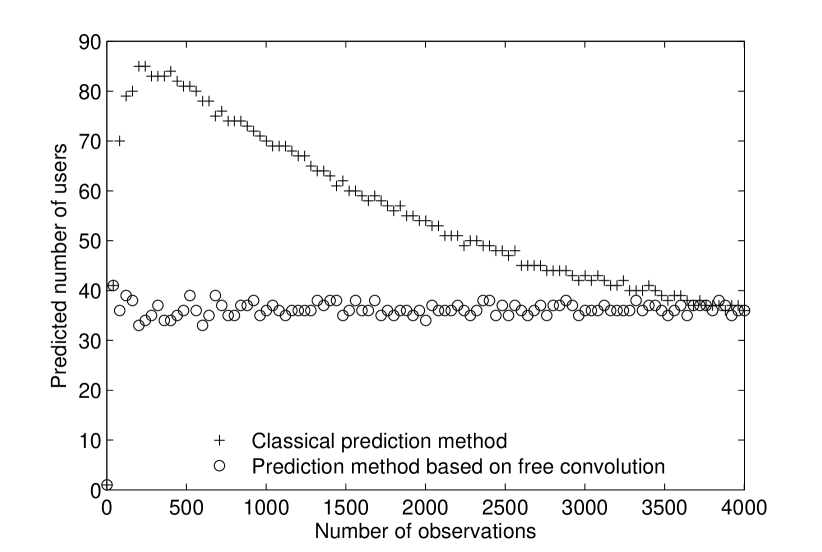
Figure 9: Estimation of the number of users with a classical method, and free convolution $L=1024$ observations have been used.

In figure 9, it is seen that when $L$ increases, we get a prediction of $N$ which is closer to the actual value $36$. The classical method starts to predict values close to the right one only for a number of observations close to $4000$. The method using free probability predicts values close to the right one for a less greater number of realizations.

V-B Estimation of Channel correlation

In channel modelling, the modeler would like to infer on the correlation between the different degrees of the channel. These typical cases are represented by a received signal (assuming that a unit training sequence has been sent) which is given by

$${\bf y}_{i}={\bf w}_{i}+{\bf b}_{i}$$ (48)

where ${\bf y}_{i}$, ${\bf w}_{i}$ and ${\bf b}_{i}$ are respectively the $n\times 1$ received vector, the $n\times 1$ zero Gaussian impulse response and $n\times 1$ additive white zero mean Gaussian noise with variance $\sigma$. The cases of interest can be:

• Ultra-wide band applications [29, 30, 31, 32] where one measures in the frequency domain the wide-band nature of the frequency signature ${\bf w}_{i}$

• Multiple antenna applications [1, 33] with one transmit and $n$ receiving antennas where ${\bf w}_{i}$ is the spatial channel signature at time instant $i$.

Usual methods compute the sample covariance matrix given by:

$$\hat{\bf R}=\frac{1}{L}\sum_{i=1}^{L}{\bf y}_{i}{\bf y}_{i}^{H}$$

The sample covariance matrix is related to the true covariance matrix of ${\bf w}_{i}$ by:

$$\hat{\bf R}={\bf\Theta}^{\frac{1}{2}}{\bf X}{\bf X}^{H}{\bf{\bf\Theta}^{\frac{1}{2}}}$$ (49)

with

$${\bf\Theta}={\bf R}+\sigma^{2}{\bf I}$$ (50)

and ${\bf X}$ is an $N\times n$ i.i.d Gaussian zero mean matrix.

Hence, if one knows the noise variance (measured without any signal sent), one can determine the eigenvalue distribution of the true covariance matrix following:

$$\mu_{\bf R}=(\mu_{\bf\hat{R}}\begin{picture}(9.0,5.0)\put(2.0,0.0){\framebox(5.0,5.0)[]{$\smallsetminus$}} \end{picture}\mu_{\frac{n}{L}})\boxminus\mu_{\sigma^{2}I}.$$ (51)

According to theorem 2, computing $\mu_{\bf\hat{R}}\begin{picture}(9.0,5.0)\put(2.0,0.0){\framebox(5.0,5.0)[]{$\smallsetminus$}} \end{picture}\mu_{\frac{n}{L}}$ is the same as computing the $G_{2}$-estimator for covariance matrices. Additive free deconvolution with $\mu_{\sigma^{2}I}$ is the same as performing a shift of the spectrum to the left.

We use a rank $K$ covariance matrix of the form ${\bf R}=diag[1,1,..,1,0,..,0]$, and variance $\sigma^{2}=0.1$, so that $\sigma\sim 0.3162$. For simulation purposes, $L$ vectors ${\bf w}_{i}$ with covariance R have been generated with $n=256$ and $K=128$. We would like to observe the p.d.f.

$$\frac{1}{2}\delta_{0}+\frac{1}{2}\delta_{1}$$ (52)

in our simulations.

In figure 10, (51) has been solved, using $L=128$ and $L=512$ observations, respectively. The same strategy as in section V-A was used, i.e. the CDF was produced by averaging eigenvalues from 100 runs. 4 moments were computed.

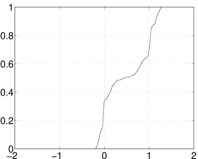
(a) $L=128$

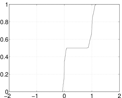
(b) $L=512$

Figure 10: CDF of eigenvalues estimated from multiplicative free deconvolution from sample covariance matrices with different number of observations.

Both cases suggest a p.d.f. close to that of (52). It is seen that the number of observations need not be higher than the dimensions of the systems in order for free deconvolution to work.

The second case corresponds to $c=0.5$, so that when there is no noise ($\sigma=0$), the sample covariance is approximately $\left(\frac{1}{2}\delta_{0}+\frac{1}{2}\delta_{1}\right)\boxtimes\mu_{\frac{1}{2}}$, which is shown in figure 6 a). If it is known that the covariance has the density $(1-p)\delta_{0}+p\delta_{\lambda}$, theorem 3 can be used, so that we only need to read the maximum density and the location parameter in order to find $p$ and $\lambda$.

It may also be that the true covariance matrix is known, and that we would like to estimate the noise variance through a limited number of observations. In figure 11, $L=128$ and $L=512$ observations have been taken.

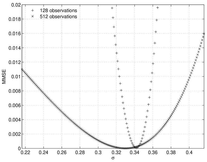
Figure 11: Estimation of the noise variance. $L=128$ and $L=512$ observations have been used.

In accordance with (51), we compute $(\mu_{\bf R}\boxplus\mu_{\eta^{2}I})\boxtimes\mu_{\frac{n}{L}}$ for a set of noise variance candidates $\eta^{2}$, and an MSE of the four first moments of this with the moments of the observed sample covariance matrix is computed. Values of $\eta$ in $(\sigma-0.1,\sigma+0.1)\sim(0.2162,0.4162)$ have been tested, with a spacing of 0.001. It is seen that the MMSE occurs close to the value $\sigma=\sqrt{0.1}=0.3162$, even if the number of observations is smaller than the rank. The MMSE occurs closer to $\sigma$ for $L=512$ than for $L=128$, so the estimate of sigma improves slightly with $L$. It is also seen that the MSE curve for $L=512$ lies lower than the MSE curve for $L=128$. An explanation for this lies in the free convolution with $\mu_{\frac{n}{L}}$: As $L\rightarrow\infty$, this has the effect of concentrating all energy at $1$.

VI Further work

In this work, we have only touched upon a fraction of the potential of free deconvolution in the field of signal processing. The framework is well adapted for any problem where one needs to infer on one of the mixing matrices. Moreover, tools were developed to practically deconvolve the measures numerically and where shown to be simple to implement. Interestingly, although the results are valid in the asymptotic case, the work presented in this paper shows that it is well suited for sizes of interest for signal processing applications. The examples draw upon some basic wireless communications problems but can be extended to other cases. In particular, classical blind methods [34, 35, 36] which assume an infinite number of observations or noisyless problems can be revisited in light of the results of this paper. The work can also be extended in several directions and should bring new insights on the potential of free deconvolution.

VI-A Other applications to signal processing

There are many other examples that could be considered in this paper. Due to limitations, we have detailed only two. For example, another case of interest can be the estimation of channel capacity. In usual measurement methods, one validates models [37, 38, 39, 40] by determining how the model fits with actual capacity measurements. In this setting, one has to be extremely cautious about the measurement noise.

Indeed, the MIMO measured channel is given by:

$$\hat{{\bf H}}_{i}=\frac{1}{\sqrt{n}}\left({\bf H}+\sigma{\bf X}_{i}\right)$$ (53)

where $\hat{\bf H}_{i}$, ${\bf H}$ and ${\bf X}_{i}$ are respectively the $n\times n$ measured MIMO matrix ($n$ is the number of receiving and transmitting antennas), the $n\times n$ MIMO channel and the $n\times n$ noise matrix with i.i.d zero mean unit variance Gaussian entries. We suppose that the channel stays constant (block fading assumption) during $L$ blocks. In this case, the observed model becomes:

$$\hat{{\bf H}}_{1...L}=\frac{1}{\sqrt{n}}\left({\bf H}_{1...L}+\frac{\sigma}{\sqrt{L}}{\bf X}_{1...L}\right)$$ (54)

with

$$\hat{{\bf H}}_{1...L}=\frac{1}{\sqrt{L}}\left[\hat{{\bf H}}_{1},\hat{{\bf H}}_{2},...,\hat{{\bf H}}_{L}\right]$$ (55)

$${\bf H}_{1...L}=\frac{1}{\sqrt{L}}\left[{\bf H},{\bf H},...,{\bf H}\right]$$ (56)

$${\bf X}_{1...L}=\left[{\bf X}_{1},{\bf X}_{2},...,{\bf X}_{L}\right]$$ (57)

The capacity of a channel with channel matrix ${\bf H}$ and signal to noise ratio $\rho=\frac{1}{\sigma^{2}}$ is given by

$$C = \frac{1}{n}\log\det\left({\bf I}+\frac{1}{n\sigma^{2}}{\bf H}{\bf H}^{H}\right).$$ (58)

$$= \frac{1}{n}\sum_{l=1}^{n}\log(1+\frac{1}{\sigma^{2}}\lambda_{l})$$ (59)

where $\lambda_{l}$ are the eigenvalues of $\frac{1}{n}{\bf H}{\bf H}^{H}$. The problem consists therefore of estimating the eigenvalues of $\frac{1}{n}{\bf H}{\bf H}^{H}$ based on few observations of $\hat{\bf H}_{i}$. For a single observation, This can be done through the approximation

$$\mu_{\hat{\bf H}_{1}\hat{\bf H}_{1}^{H}}\begin{picture}(9.0,5.0)\put(2.0,0.0){\framebox(5.0,5.0)[]{$\smallsetminus$}} \end{picture}\mu_{1}=\left(\mu_{\frac{1}{n}{\bf H}{\bf H}^{H}}\begin{picture}(9.0,5.0)\put(2.0,0.0){\framebox(5.0,5.0)[]{$\smallsetminus$}} \end{picture}\mu_{1}\right)\boxplus\mu_{\sigma}.$$ (60)

If we have many observations, we have that:

$$\mu_{\hat{\bf H}_{1...L}\hat{\bf H}_{1...L}^{H}}\begin{picture}(9.0,5.0)\put(2.0,0.0){\framebox(5.0,5.0)[]{$\smallsetminus$}} \end{picture}\mu_{1}=\left(\mu_{\frac{1}{n}{\bf H}{\bf H}^{H}}\begin{picture}(9.0,5.0)\put(2.0,0.0){\framebox(5.0,5.0)[]{$\smallsetminus$}} \end{picture}\mu_{1}\right)\boxplus\mu_{\frac{\sigma}{\sqrt{L}}}.$$ (61)

VI-B Other types of sample matrices

One topic of interest is the use of free deconvolution with other types of matrices than the sample covariance matrix. In fact, based on a given set of observations, one can construct higher sample moment matrices than the sample covariance matrix (third product matrix for example). These matrices contain useful information that could be used in the problem. The main difficult issue here is to prove freeness of the convolved measures. The free deconvolution framework could also be applied to tensor problems [41] and this has not been considered yet to our knowledge.

VI-C Colored Noise

In this work, the noise considered was supposed to be temporally and spatially white with standard Gaussian entries. This yields the Marc̆henko pastur law as the operand measure. However, the analysis can be extended, with the assumption that freeness is proved, to other type of noises: the case for example of an additive noise with a given correlation. In this case, the operand measure is not the Marc̆henko pastur law but depends on the limiting distribution of the sample noise covariance matrix. Although the mathematical formulation turns out to be identical, in terms of implementation, the problem is more complicated as one has to use more involved power series than the $Zeta$-series for example.

VI-D Parametrized distribution

In the previous example (signal impaired with noise), the Marc̆henko Pastur law $\mu_{c}$ was one of the operand measures, while the other was either estimated or considered to be a discrete measure, i.e. with density

$$f^{\mu}(x)=\sum_{i=1}^{n}p_{i}\delta_{\lambda_{i}}(x).$$ (62)

It turns out that one can find also the parameterized distribution (best fit by adjusting the parameter) that deconvolves up to certain minimum mean square error. For example, one could approximate the measure of interest with two diracs (instead of the set of $n$ diracs) and find the best set of diracs that minimizes the mean square error. One can also approximate the measure with the Marc̆henko pastur law for which the parameter $c$ needs to be optimized. In both cases, the interesting point is that the expressions can be derived explicitly.

VII Conclusion

In this paper, we have shown that free probability provides a neat framework for estimation problems when the number of observations is of the same order as the dimensions of the problem. In particular, we have introduced a free deconvolution framework (both additive and multiplicative) which is very appealing from a mathematical point of view and provides an intuitive understanding of some G-estimators provided by Girko [11]. Moreover, implementation aspects were discussed and proved to be adapted, through simulations, to classical signal processing applications without the need of infinite dimensions.

Appendix A Algorithm for computing free convolution

The files momcum.m and cummom.m in [25] are implementations of (24) in MATLAB. The first calculates cumulants from moments, the second moments from cumulants. Both programs are rather short, and both take a series of moments $(\mu_{1},...,\mu_{n})$ as input. The algorithm for computing cumulants from moments goes the following way:

1. Form the vector $m=(1,\mu_{1},...,\mu_{n})$ of length $n+1$, and compute and store recursively the $n$ vectors

   $$M_{1}=m\mbox{, }M_{2}=m\star m\mbox{,..., }M_{n}=\star_{n}m,$$

   where $\star_{n}$ stands for $n$-fold (classical) convolution with itself. The later steps in the algorithm use only the $n+1$ first elements of the vectors $M_{1}$, $M_{2}$,…,$M_{n}$. Consequently, the full $M_{k}$ vectors are not needed for all $k$: We can truncate $M_{k}$ to the first $n+1$ elements after each convolution, so that the implementation can be made quite efficient.

2. Calculate the cumulants recursively. If the first $n-1$ cumulants, i.e. the first $\alpha_{i}$ in (24), have been found by solving the $n-1$ first equations in (24), $\alpha_{n}$ can then be found through the $n$th equation in (24), by using the vectors computed in step 1). More precisely ,the connection between the vectors in 1) and the value we use in (24) is

   $$coef_{n-k}\left(\left(1+\mu_{1}z+\mu_{2}z^{2}+...\right)^{k}\right)=M_{k}(n-k),$$

   where $n-k$ denotes the index in the vector (starting from $0$). Finding the $k$’th cumulant $\alpha_{k}$ by solving the $k$th equation in (24) is the same as

   $$\alpha_{k}=\frac{M_{1}(n+1)-\sum_{1\leq r\leq k-1}\alpha_{r}M_{r}(k-r)}{M_{k}(0)}.$$

The program for computing moments from cumulants is slightly more complex, since we can’t start out by computing the vectors $M_{1}$,…,$M_{n}$ separately at the beginning, since the moments are used to form them (these are not known yet). Instead, elements in $M_{1}$,…,$M_{n}$ are added each time a new moment has been computed.

Appendix B The proof of theorem 3

Set $\eta(z)=\eta_{\mu\boxtimes\mu_{c}}$. From (37) we see that we must solve the equation

$$\eta_{\mu}\left(z(1-c+c\eta(z))\right)=\eta(z).$$

Substituting (39), multiplying and collecting terms, we get that $\eta(z)$ must be a zero for the equation

$$cz\lambda\eta(z)^{2}+\left(1+z\lambda(1-2c+cp))\right)\eta(z)-(1-p)(1-c)z\lambda-1.$$

The analytical continuation of $m(z)=m_{\mu\boxtimes\mu_{c}}(z)$ to the negative part of the real line satisfies $\eta(z)=\frac{m\left(-\frac{1}{z}\right)}{z}$. Subsituting this and also substituting $u=-\frac{1}{z}$, we get that

$$-c\lambda zm(z)^{2}+(\lambda(1-2c+cp)-z)m(z)+\frac{1}{z}\lambda(1-p)(1-c)-1$$ (63)

equals $0$ for $z$ which are real and negative. It is clear that any analytical continuation of $m(z)$ to the upper half of the complex plane also must satisfy (63). We use the formula for the solution of the second degree equation and get that $m(z)$ equals

$$\begin{array}[]{ll}&\frac{-\lambda(1-2c+cp)+z\pm\sqrt{\begin{array}[]{l}(\lambda(1-2c+cp)-z)^{2}\\ +4c\lambda^{2}(1-p)(1-c)-4c\lambda z\end{array}}}{-2c\lambda z}\\ &=\frac{(\lambda(1-2c+cp)+z\mp\sqrt{\begin{array}[]{l}z^{2}-2\lambda(1+cp)z\\ +4c\lambda^{2}(1-c)(1-p)\\ +\lambda^{2}(1-2c+cp)^{2}\end{array}}}{2c\lambda z}.\end{array}$$ (64)

The zeroes of the discriminant here are

$$\begin{array}[]{lll}&&\frac{2(\lambda(1+cp)\pm\sqrt{\lambda^{2}4(1+cp)^{2}-16c\lambda^{2}(1-c)(1-p)-4\lambda^{2}(1-2c+cp)^{2}}}{2}\\ &=&\lambda(1+cp)\\ &&\pm\frac{1}{2}\lambda\sqrt{\begin{array}[]{l}4(1+cp)^{2}-16c(1-c)(1-p)\\ -4(1+cp)^{2}-16c^{2}+16c(1+cp)\end{array}}\\ &=&\lambda(1+cp)\pm\frac{1}{2}\lambda\sqrt{16c(1+cp-c-(1-c)(1-p))}\\ &=&\lambda(1+cp)\pm 2\lambda\sqrt{cp},\end{array}$$

This means that we can rewrite $m(z)$ to

$$\frac{\lambda(1-2c+cp)+z\mp\sqrt{\begin{array}[]{l}(z-\lambda(1+cp)+2\lambda\sqrt{cp})\\ (z-\lambda(1+cp)-2\lambda\sqrt{cp})\end{array}}}{2c\lambda z}.$$

Thus, for $z$ real, $m(z)$ is complex if and only if $z$ lies in the interval $I_{\lambda,c,p}$ of (31). Outside $I_{\lambda,c,p}$, the density of $\mu\boxtimes\mu_{c}$ is zero. Taking the imaginary part and using the Stieltjes inversion formula, we get that the density in $I_{\lambda,c,p}$ is given by the formula (32).

Setting the derivative of (32) w.r.t. $z$ equal to $z$ gives us a first degree equation which yields a unique maximum at $z=\lambda\frac{(1-cp)^{2}}{1+cp}$. After some more calculations, we get that the density at this extremal point is $\frac{\sqrt{cp}}{c\pi\lambda(1-cp)}$. This finishes the proof.             

Appendix C The proof of theorem 4

Set $\eta(z)=\eta_{\mu\begin{picture}(9.0,5.0)\put(2.0,0.0){\framebox(5.0,5.0)[]{$\smallsetminus$}} \end{picture}\mu_{c}}$, we see from (38) that we must solve the equation

$$\eta_{\mu}\left(\frac{z}{1-c+c\eta(z)}\right)=\eta(z).$$

Substituting (39), multiplying and collecting terms, we get that $\eta(z)$ must be a zero for the equation

$$c\eta(z)^{2}+(1-2c+z\lambda)\eta(z)-(1-c)-z\lambda(1-p).$$

Using the formula for the solution of the second degree equation, one can see that the positive square root must be chosen whenever $c<\frac{1}{2}$, since $\eta$ assumes positive positive values whenever $z\geq 0$. Substituting $\eta(z)=\frac{m\left(-\frac{1}{z}\right)}{z}$ and also $u=-\frac{1}{z}$ as in the case for convolution, we get that

$$cz^{2}m(z)^{2}+(\lambda-z(1-2c))m(z)+\frac{1}{z}\lambda(1-p)-(1-c)$$

equals $0$ for $z$ which are real and negative. We get that $m(z)$ equals

$$\begin{array}[]{ll}&\frac{-\lambda+z(1-2c)\pm\sqrt{\begin{array}[]{l}(\lambda-z(1-2c))^{2}\\ -4cz^{2}\left(\frac{1}{z}\lambda(1-p)-(1-c)\right)\end{array}}}{2cz^{2}}\\ &=\frac{-\lambda+z(1-2c)\pm\sqrt{z^{2}-2\lambda(1-2cp)z+\lambda^{2}}}{2cz^{2}}.\end{array}$$ (65)

The zeroes of the discriminant are

$$\begin{array}[]{ll}&\frac{2\lambda(1-2cp)\pm\sqrt{4\lambda^{2}(1-2cp)^{2}-4\lambda^{2}}}{2}\\ =&\lambda(1-2cp)\pm\frac{1}{2}\sqrt{4\lambda^{2}(4c^{2}p^{2}-4cp)^{2}}\\ =&\lambda(1-2cp)\pm 2\lambda\sqrt{cp(1-cp)}.\end{array}$$

Following the same reasoning as for convolution, we see that the density is $0$ outside the interval $J_{\lambda,c,p}$ of (33), and that the density in $J_{\lambda,c,p}$ is given by (34). This finishes the proof.

References

- [1] E. Telatar, “Capacity of Multi-Antenna Gaussian Channels,” Eur. Trans. Telecomm. ETT, vol. 10, no. 6, pp. 585–596, Nov. 1999.
- [2] D. Tse and S. Hanly, “Linear multiuser receivers: Effective interference, effective bandwidth and user capacity,” IEEE Transactions on Information Theory, vol. 45, no. 2, pp. 641–657, 1999.
- [3] S. Shamai and S. Verdu, “The Impact of Frequency-Flat Fading on the Spectral Efficiency of CDMA,” pp. 1302–1326, May 2001.
- [4] S. Verdu and S. Shamai, “Spectral Efficiency of CDMA with Random Spreading,” pp. 622–640, Mar. 1999.
- [5] T. Guhr, A. Müller-Groeling, and H. Weidenmüller, “Random Matrix Theories in Quantum Physics: Common Concepts,” Physica Rep., pp. 190–, 299 1998.
- [6] M. Mehta, Random Matrices, 2nd ed. New York: Academic Press, 1991.
- [7] J.-P. Bouchaud and M. Potters, Theory of Financial Risks-From Statistical Physics to Risk Management. Cambridge: Cambridge University Press, 2000.
- [8] S. Gallucio, J.-P. bouchaud, and M. Potters, “Rational Decisions, Random Matrices and Spin Glasses,” Physica A, pp. 449–456, 259 1998.
-
[9]
B. Dozier and J. Silverstein, “On the empirical distribution of eigenvalues of
large dimensional information-plus-noise type matrices,” Submitted.,
2004, http://www4.ncsu.edu/
~jack/infnoise.pdf. -
[10]
Ø. Ryan, “Multiplicative free convolution and information-plus-noise type
matrices,” Planned for submission to Journal Of Functional Analysis,
2006, http://www.ifi.uio.no/
~oyvindry/multfreeconv.pdf. - [11] V. L. Girko, “Ten years of general statistical analysis,” http://general-statistical-analysis.girko.freewebspace.com/chapter14.pdf.
- [12] X. Mestre, “Designing good estimators for low sample sizes: random matrix theory in array processing applications,” in 12th European Signal Processing Conference, (EUSIPCO’2004), Sept. 2004.
- [13] N. Rao and A. Edelman, “Free probability, sample covariance matrices and signal processing,” ICASSP, pp. 1001–1004, 2006.
- [14] F. Hiai and D. Petz, The Semicircle Law, Free Random Variables and Entropy. American Mathematical Society, 2000.
- [15] D. Voiculescu, “Addition of certain non-commuting random variables,” J. Funct. Anal., vol. 66, pp. 323–335, 1986.
- [16] D. V. Voiculescu, “Multiplication of certain noncommuting random variables,” J. Operator Theory, vol. 18, no. 2, pp. 223–235, 1987.
- [17] D. Voiculescu, “Circular and semicircular systems and free product factors,” vol. 92, 1990.
- [18] ——, “Limit laws for random matrices and free products,” Inv. Math., vol. 104, pp. 201–220, 1991.
- [19] V. L. Girko, “Circular Law,” Theory. Prob. Appl., pp. 694–706, vol. 29 1984.
- [20] Z. D. Bai, “The Circle Law,” The Annals of Probability., pp. 494–529, 1997.
- [21] A. Tulino and S. Verdo, Random Matrix Theory and Wireless Communications. www.nowpublishers.com, 2004.
- [22] V. L. Girko, Statistical Analysis of Observations of Increasing Dimension. Kluwer Academic Publishers, 1995.
- [23] S. T. rnsen, “Mixed moments of voiculescu’s gaussian random matrices,” J. Funct. Anal., vol. 176, no. 2, pp. 213–246, 2000.
- [24] A. Nica and R. Speicher, Lectures on the Combinatorics of Free Probability. Cambridge University Press, 2006.
-
[25]
Ø. Ryan, Computational tools for free convolution, 2006,
http://ifi.uio.no/
~oyvindry/freedeconvsignalprocapps/. -
[26]
O. Ryan, “Implementation of free deconvolution,” Planned for submission
to IEEE Transactions on Signal Processing, 2006,
http://www.ifi.uio.no/
~oyvindry/freedeconvsigprocessing.pdf. - [27] R. Seroul and D. O’Shea, Programming for Mathematicians. Springer.
- [28] J. Silverstein and P. Combettes, “Signal detection via spectral theory of large dimensional random matrices,” IEEE Transactions on Signal Processing, vol. 40, no. 8, pp. 2100–2105, 1992.
- [29] I. E. Telatar and D. N. C. Tse, “Capacity and Mutual Information of Wideband Multipath Fading Channels,” IEEE Transactions on Information Theory, pp. 1384 –1400, July 2000.
- [30] D. Porrat, D. N. C. Tse, and S. Nacu, “Channel Uncertainty in Ultra Wide Band Communication Systems,” IEEE Transactions on Information Theory, submitted 2005.
- [31] W. Turin, R. Jana, S. Ghassemzadeh, C. Rice, and T. Tarokh, “Autoregressive modelling of an indoor UWB radio channel,” IEEE Conference on Ultra Wideband Systems and Technologies, pp. 71 – 74, May. 2002.
- [32] R. L. de Lacerda Neto, A. M. Hayar, M. Debbah, and B. Fleury, “A Maximum Entropy Approach to Ultra-Wide Band Channel Modelling,” International Conference on Acoustics, Speech, and Signal Processing, May 2006.
- [33] D. Gesbert, M. Shafi, D. Shiu, P. Smith, and A. Naguib, “From Theory to Practice: an Overview of MIMO Space-Time Coded Wireless Systems,” pp. 281– 302, vol. 21, no. 3 2003.
- [34] D. Donoho, “On minimum entropy deconvolution,” In Applied Time-series analysis II, p-565-609, Academic Press, 1981.
- [35] P. Comon, “Independent component analysis, a new concept?” Signal Processing, Elsevier, 36(3):287–314, Special issue on Higher-Order Statistics, Apr. 1994.
- [36] A. Belouchrani, K. A. Meraim, J.-F. Cardoso, and E. Moulines, “A blind source separation technique based on second order statistics,” IEEE Transactions on Signal Processing, 45(2):434-44, Feb. 1997.
- [37] J. Kermoal, L. Schumacher, K. Pedersen, P. Mogensen, and F. Frederiken, “A Stochastic MIMO Radio Channel Model with Experimental Validation,” pp. 1211–1225, vol. 20, no. 6 2002.
- [38] H. Ozcelik, M. Herdin, W. J. Weichselberg, and E. Bonek, “Deficiencies of ”Kronecker” MIMO Radio Channel Model,” IEE Electronics Letters, vol. 39, no. 16, pp. 1209–1210, Aug. 2003.
- [39] H. Ozcelik, N. Czink, and E. Bonek, “What Makes a good MIMO Channel Model,” Proceedings of the IEEE VTC conference, 2005.
- [40] M. Debbah, R. Müller, H. Hofstetter, and P. Lehne, “What determines Mutual Information on MIMO channels,” second round review, IEEE Transactions on Wireless Communications, 2006.
- [41] J. B. Kruskal, “Three-way arrays: rank and uniqueness of trilinear decompositions, with applications to arithmetic complexity and statistics,” Linear Algebra Applicat., vol. 18, pp. 95-138, 1977.