Flow-optimized Cooperative Transmission for the Relay Channel

Abstract

This paper describes an approach for half-duplex cooperative transmission in a classical three-node relay channel. Assuming availability of channel state information at nodes, the approach makes use of this information to optimize distinct flows through the direct link from the source to the destination and the path via the relay, respectively. It is shown that such a design can effectively harness diversity advantage of the relay channel in both high-rate and low-rate scenarios. When the rate requirement is low, the proposed design gives a second-order outage diversity performance approaching that of full-duplex relaying. When the rate requirement becomes asymptotically large, the design still gives a close-to-second-order outage diversity performance. The design also achieves the best diversity-multiplexing tradeoff possible for the relay channel. With optimal long-term power control over the fading relay channel, the proposed design achieves a delay-limited rate performance that is only $3.0$dB ($5.4$dB) worse than the capacity performance of the additive white Gaussian channel in low- (high-) rate scenarios.

I Introduction

It is well known that the performance of a wireless network can be significantly improved by cooperative transmission among nodes in the network. Many cooperative transmission designs aim to exploit cooperative diversity that is inherently present in the network. Such designs have been suggested in [1, 2] for cellular networks. Recently there has been much interest in achieving cooperative diversity in a classical three-node relay channel [3], which represents the simplest wireless network that can derive advantages from cooperative transmission.

The relay channel has been thoroughly studied in [3]. Bounds on the capacity have been given for the general relay channel, and the capacity has been calculated for the special case of degraded relay channels. The coding techniques suggested in [3] assume that the relay can operate in a full-duplex manner; i.e., it can transmit and receive at the same time. It is commonly argued that full-duplex operation is not practical for most existing wireless transceivers. Thus the restriction of half-duplex operation at the relay is usually considered in cooperative transmission designs.

Since the relay cannot transmit and receive simultaneously, a time-division approach is employed in half-duplex relaying [4]. The source first transmits to the destination, and the relay listens and “captures” [5] the transmission from the source at the same time. Then the relay aids the transmission by sending processed source information to the destination. Note that the source may still send data to the destination when the relay transmits. Several techniques to process and forward the received data by the relay have been suggested. These techniques include the decode-and-forward (DF) and amplify-and-forward (AF) approaches [4]. In the DF approach, the relay decodes the received signal from the source and then forwards a re-encoded signal to the destination. In the AF approach, the relay simply amplifies and forwards the signal received from the source to the destination.

The performance of the DF approach is limited by the capability of the relay to correctly decode the signal received from the source. This in turn depends on the quality of the link from the source to the relay. On the other hand, the AF approach performs poorly in low signal-to-noise ratio (SNR) situations in which the relay forwards mainly noise to the destination. In addition, the time-division approach leads to rate losses that are significant when the relay channel is to support high rates. Some enhanced versions of the AF and DF approaches have been proposed to solve the rate loss problem. A distributed space-time-coding protocol is developed in [6]. An incremental AF technique which requires feedback from the destination to the source is developed in [4]. The non-orthogonal AF and dynamic DF techniques suggested in [7] allow the duration of the relay listening to the transmission from the source to adapt to the condition of the link from the source to the relay. In particular, the dynamic DF technique is shown to be superior to all the cooperative diversity techniques (except perhaps the incremental relaying techniques) mentioned above. A bursty AF technique is also suggested in [8] to solve the noise forwarding problem of the AF approach when the SNR is low. It is shown that the bursty AF technique achieves the best outage performance at the asymptotically low SNR regime. We note that all these cooperative diversity techniques mentioned so far are designed with the constraint that channel state information is not available at the source and the relay. Some practical code designs for the DF and space-time-coding approaches have been suggested in [9] and [10], respectively.

When the links in the relay channel suffer from slow fading, it is conceivable that the channel state information (or at least the channel quality information) can be estimated and passed to the nodes. The source and relay may then use this information to optimize the cooperative protocol to achieve better performance. Such a design has been considered in [5], in which optimal power control is performed at the source and relay in order to maximize the ergodic rates achieved by the DF and compress-forward approaches.

In this paper, we assume that the channel state information is available, and we develop time-division cooperative diversity designs that perform well in both high-rate and low-rate scenarios. The main distinguishing feature of the proposed approach, compared with the cooperative designs mentioned above, is that we do not employ the approach of the relay “capturing” the transmission from the source to the destination. Instead, we divide the information to be sent to the destination into three flows. The source employs cooperative broadcasting [11, 12] to intentionally send two distinct flows of data to the relay and destination, respectively, in the first time slot. The relay helps to forward, in the DF manner, the data that it receives to the destination in the second time slot, during which the source concurrently sends the remaining flow of data to the destination. The transmit powers of the source and relay as well as the durations of the time slots are optimized according to the link conditions and the rate requirement. This constitutes a form of optimal flow control.

Due to the DF nature of the proposed design, there is an implicit restriction on the decoding delay. Thus we will employ the capacity-versus-outage framework [13, 14] to evaluate the performance of the proposed design. We will show that the proposed design can efficiently achieve cooperative diversity in both high-rate and low-rate scenarios. In particular, when the rate requirement is asymptotically small, the outage performance of the proposed design approaches that of full-duplex relaying with DF, giving a second-order diversity performance. On the other hand, when the rate requirement is asymptotically large, the proposed approach still gives a close-to-second-order diversity performance. Moreover, the design also gives the best diversity-multiplexing tradeoff [15] possible for the relay channel. Together with the application of optimal long-term power control [16], the design can give very good delay-limited rate performance again in both low-rate and high-rate scenarios.

We note that the two basic building blocks for the proposed approach are cooperative broadcasting (CB) in the first time slot and multiple access (MA) in the second time slot. The combination of CB and MA allows distinct flows of data be sent through the relay and through the direct link from the source to the destination, and hence can be viewed as a generalized form of routing. A practical advantage of the proposed design is that the basic building blocks are the well known CB and MA approaches. Practical MA coding designs have been well studied, e.g. see [17, 18], while practical CB coding designs are currently available [19]–[21].

II Relay Channel: Full-Duplex Bounds

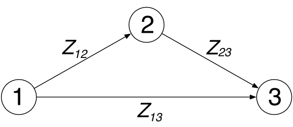
Figure 1: The classical 3-node relay channel.

Consider a classical three-node relay network, which consists of a source node 1, a relay node 2, and a destination node 3 as shown in Fig. 1. We assume that each link in the figure is a bandpass Gaussian channel with bandwidth $W$ and one-sided noise spectral density $N_{0}$. Let $Z_{ij}$ denote the power gain of the link from node $i$ to node $j$. The link power gains are assumed to be independent and identically distributed (i.i.d.) exponential random variables with unit mean. This corresponds to the case of independent Rayleigh fading channels with unit average power gains. The results in the sequel can be easily generalized to include the case of non-uniform average power gains.

In this section, we consider the case in which the relay node is capable of supporting full-duplex operation. Our goal is to support an information rate of $K$ nats/s/Hz from the source to the destination. We assume that the link power gains change slowly so that they can be estimated, and hence the power gain information is available at all nodes. The source and relay nodes can make use of this information to control their respective transmit power and time so that the total transmit energy is minimized. For convenience, we consider a slotted communication system with unit-duration time slots. Let $P_{t}$ be the total transmit energy of the source and relay needed to support the transmission of $KW$ nats of information from the source to the destination in a time slot. Since the duration of a time slot is one, $P_{t}$ is also the total average transmit power required. Although interpreting $P_{t}$ as the total average power may not carry any significant physical meaning, it is customary to speak of “power” rather than “energy” in for communication engineers. Unless otherwise stated, we will hereafter consider a normalized version of $P_{t}$, namely the rate-normalized overall signal-to-noise ratio (RNSNR) of the network:

$$S\stackrel{{\scriptstyle\triangle}}{{=}}\frac{P_{t}}{N_{0}W}\frac{1}{e^{K}-1}.$$

The RNSNR can be interpreted as the additional SNR, in dB, needed to support the required rate of $K$ nats/s/Hz, in excess of the SNR required to support the same rate in a simple Gaussian channel with unit gain. This normalization is convenient as we will consider asymptotic cases when $K$ approaches zero and infinity.

We note that the use of the RNSNR to characterize our results has two important implications. First, since the total transmit energy of the source and relay is used in defining the RNSNR, no individual power limits are put on the source and relay. The results in this paper can be viewed as bounds if additional individual power limits are imposed. Our choice of focusing on the total energy comes from the viewpoint that the relay channel considered forms a small component of a larger wireless network. In this sense, it is fairer to compare the total transmit energy incurred in sending information from the source to the destination by employing cooperative diversity to that incurred in direct transmission. Second, the normalization by the factor $e^{K}-1$ implies that the additional SNR in dB to combat fading can only be a constant over the SNR required to achieve the target rate in a Gaussian channel, regardless of the rate requirement. That is, we restrict the SNR to increase at the same rate as in a Gaussian channel to cope with increases in the transmission rate through the relay channel. In a sense, this restriction enforces efficiency of energy usage.

Employing well known capacity bounds on the relay channel [5, 3, 22], we can obtain the following bounds on the RNSNR to support required spectral efficiency of $K$nats/s/Hz.

Theorem II.1

For any fixed positive link power gains $Z_{12}$, $Z_{13}$, and $Z_{23}$, define the bound

$$B_{\mathrm{DF}}\stackrel{{\scriptstyle\triangle}}{{=}}\left\{\begin{array}[]{ll}\displaystyle{\frac{Z_{12}+Z_{23}}{Z_{12}(Z_{13}+Z_{23})}}&\mbox{~{}if~{}}Z_{12}>Z_{13}\\ \displaystyle{\frac{1}{Z_{13}}}&\mbox{~{}otherwise,}\end{array}\right.$$

and

$$B_{\mathrm{lb}}\stackrel{{\scriptstyle\triangle}}{{=}}\displaystyle{\frac{Z_{12}+Z_{13}+Z_{23}}{(Z_{12}+Z_{13})(Z_{13}+Z_{23})}}.$$

Then $S>B_{\mathrm{DF}}$ is a sufficient condition in order to support the rate of $K$nats/s/Hz from the source to destination. Also $S\geq B_{\mathrm{lb}}$ is a necessary condition in order to support the rate of $K$nats/s/Hz from the source to destination.

Proof:

See Appendix -A. ∎

The RNSNR $B_{\textrm{DF}}$ is achieved by the DF approach employing the block Markov coding suggested in [3, 22]. We also need to optimally allocate transmit energy between the source and relay nodes. In addition, the availability of channel state information (both magnitudes and phases of the fading coefficients of all three links) as well as symbol timing and carrier phase synchronization at all the three nodes are implicitly assumed. The lower bound $B_{\textrm{lb}}$ is based on the max-flow-min-cut bound in [22]. No known coding technique can achieve this bound.

III Half-Duplex Protocols based on Flow Control

In this section, we will consider the more practical scenario in which the relay node operates in the following half-duplex fashion. We partition each unit time slot into two sub-slots with respective durations $t_{1}$ and $t_{2}$, where $t_{1}+t_{2}=1$. In the first time slot, the source transmits while the relay and destination receive. In the second time slot, the source and relay transmit, and the destination receives. Based on this half-duplex mode of operation, we will describe two cooperative communication protocols that make use of the two basic components of cooperative broadcasting (CB) from the source to the relay in the first time slot and multiple access (MA) from the source and relay in the second time slot. The first protocol does not require phase synchronization among the three nodes, while the second protocol does so.

III-A Half-Duplex Protocol 1 (HDP1)

In this protocol, the information from the source to the destination is divided into three flows of data $x_{1}$, $x_{2}$, and $x_{3}$, where $x_{1}+x_{2}+x_{3}=K$. In the first time slot, the source sends, via CB, two flows of rates $x_{1}/t_{1}$ and $x_{2}/t_{1}$ to the destination and relay, respectively. In the second time slot, the relay and source send, via MA, two flows of rates $x_{2}/t_{2}$ and $x_{3}/t_{2}$ to the destination, respectively. The information flow of rate $x_{2}/t_{2}$ sent by the relay in the second time slot is from the flow of rate $x_{2}/t_{1}$ that it receives and decodes in the first time slot. We choose $t_{1}$, $t_{2}$, $x_{1}$, $x_{2}$, and $x_{3}$ to minimize the total power transmitted by the source and relay to support the rate $K$nats/s/Hz from the source to the destination.

To determine the minimum RNSNR that can support the required rate when this protocol is employed, we start with the following lemma.

Lemma III.1

1. For $0<t_{1}\leq 1$, the infimum of the SNR required so that the source can broadcast at rates $x_{1}/t_{1}$ and $x_{2}/t_{1}$ to the destination and relay, respectively, in the first time slot is

   $$S_{\textrm{CB}}=\left\{\begin{array}[]{ll}\displaystyle\frac{1}{Z_{12}}(e^{x_{2}/t_{1}}-1)+\frac{1}{Z_{13}}e^{x_{2}/t_{1}}(e^{x_{1}/t_{1}}-1)&\mathrm{~{}if~{}}Z_{13}\geq Z_{12},\\ \displaystyle\frac{1}{Z_{13}}(e^{x_{1}/t_{1}}-1)+\frac{1}{Z_{12}}e^{x_{1}/t_{1}}(e^{x_{2}/t_{1}}-1)&\mathrm{~{}otherwise}.\end{array}\right.$$

   For $t_{1}=0$, $S_{\textrm{CB}}=0$.

2. For $0<t_{2}\leq 1$, the infimum of the SNR required so that the source and relay can simultaneously transmit at rates $x_{3}/t_{2}$ and $x_{2}/t_{2}$, respectively, to the destination in the second time slot is

   $$S_{\textrm{MA}}=\left\{\begin{array}[]{ll}\displaystyle\frac{1}{Z_{23}}(e^{x_{2}/t_{2}}-1)+\frac{1}{Z_{13}}e^{x_{2}/t_{2}}(e^{x_{3}/t_{2}}-1)&\mathrm{~{}if~{}}Z_{13}\geq Z_{23},\\ \displaystyle\frac{1}{Z_{13}}(e^{x_{3}/t_{2}}-1)+\frac{1}{Z_{23}}e^{x_{3}/t_{2}}(e^{x_{2}/t_{2}}-1)&\mathrm{~{}otherwise}.\end{array}\right.$$

   For $t_{2}=0$, $S_{\textrm{MA}}=0$.

Proof:

See Appendix -B. ∎

With the help of Lemma III.1, we can now formulate the optimization of the parameters in Protocol 1 as follows:

$$\begin{array}[]{lll}&\min\ t_{1}S_{\textrm{CB}}+t_{2}S_{\textrm{MA}}&\\ \mbox{subject~{}to}&\mbox{i. total data requirement:}&x_{1}+x_{2}+x_{3}=K\\ &\mbox{ii. total time requirement:}&t_{1}+t_{2}=1\\ &\mbox{iii. non-negativity requirements:}&x_{1},x_{2},x_{3},t_{1},t_{2}\geq 0\end{array}$$ (1)

where $S_{CB}$ and $S_{MA}$ are of the forms in Lemma III.1. It is not hard to see that (1) is a convex optimization problem and its solution provides the tightest lower bound for the SNR required to support the rate of $K$nats/s/Hz:

Theorem III.1

Let $B_{1}(K)$ be the minimum value achieved in the optimization problem (1), normalized by the factor $e^{K}-1$. Then $B_{1}(K)$ is the infimum of the RNSNR required so that the rate of $K$nats/s/Hz can be supported from the source to the destination by HDP1.

III-A1 Description of $B_{1}(K)$

To describe the form of the RNSNR bound $B_{1}(K)$, we need to consider the following few cases. This solution is established by applying the Karush-Kuhn-Tucker (KKT) condition [23] to the convex optimization problem (1) as detailed in Appendix -C. For notational convenience, we write

$$M_{H}(x,y)=\frac{1}{\frac{1}{x}+\frac{1}{y}}$$

as the harmonic mean of two real numbers $x$ and $y$.

$Z_{13}\geq M_{H}(Z_{12},Z_{23})$

The solution is given by

$$\begin{array}[]{l}x_{1}=Kt_{1},\\ x_{2}=0,\\ x_{3}=Kt_{2},\end{array}$$

where $t_{1}$ and $t_{2}$ can be arbitrarily chosen as long as they satisfy the non-negativity and total-time requirements. This corresponds to directly transmitting all data through the link from the source to destination, without utilizing the relay. The resulting value of $B_{1}(K)$ is

$$B_{1}(K)=\frac{1}{Z_{13}}.$$

$Z_{13}<M_{H}(Z_{12},Z_{23})$

Define

$$A_{1} = Z_{23}\left(\frac{1}{Z_{13}}-\frac{1}{Z_{12}}\right),$$

$$A_{2} = Z_{12}\left(\frac{1}{Z_{13}}-\frac{1}{Z_{23}}\right).$$

Notice that $A_{1}>1$ and $A_{2}>1$. Consider two sub-cases:

1. $K>M_{H}(\log A_{1},\log A_{2})$:
   In this case,

   $$B_{1}(K)=\frac{\min\{\tilde{S}_{1}(K),\tilde{S}_{2}(K),\tilde{S}_{3}(K)\}}{e^{K}-1},$$ (2)

   where the three SNR terms $\tilde{S}_{1}(K)$, $\tilde{S}_{2}(K)$, and $\tilde{S}_{3}(K)$ are respectively defined in (3), (4), and (5) below.

   The first SNR term is given by

   $$\tilde{S}_{1}(K)=\min_{\max\left\{0,1-\frac{K}{\log A_{1}}\right\}\leq t_{1}\leq\min\left\{\frac{K}{\log A_{2}},1\right\}}\left\{\frac{1}{Z_{12}}e^{K+(1-t_{1})\log A_{2}}+\frac{1}{Z_{23}}e^{K+t_{1}\log A_{1}}-\frac{1}{Z_{13}}\right\}.$$ (3)

   Define

   $$t^{*}=\frac{\log\left(\displaystyle\frac{Z_{23}\log A_{2}}{Z_{12}\log A_{1}}\right)+\log A_{2}}{\log A_{1}+\log A_{2}}.$$

   Employing the well known inequalities $\log x\leq x-1$ for $x\geq 1$ and $\log x\geq 1-\frac{1}{x}$ for $x>0$, it can be shown that $0\leq t^{*}\leq 1$. By simple calculus, $t^{*}$ is the minimizing $t_{1}$ in (3) above when $\max\left\{0,1-\frac{K}{\log A_{1}}\right\}\leq t^{*}\leq\min\left\{\frac{K}{\log A_{2}},1\right\}$. When $t^{*}$ lies outside that range, the minimizing $t_{1}$ must be one of the boundary points. When $\tilde{S}_{1}(K)$ is the minimum among the three terms inside the $\min$ operator in (2), the corresponding solution to the optimization problem (1) is given by

   $$\begin{array}[]{l}x_{1}=Kt^{*}-t^{*}(1-t^{*})\log A_{1},\\ x_{2}=t^{*}(1-t^{*})\log(A_{1}A_{2}),\\ x_{3}=K(1-t^{*})-t^{*}(1-t^{*})\log A_{2},\end{array}$$

   with $t_{1}=t^{*}$ and $t_{2}=1-t^{*}$.

   The second SNR term is given by

   $$\tilde{S}_{2}(K)=\min_{\min\left\{\frac{K}{\log A_{2}},1\right\}\leq t_{1}\leq 1}\left\{\frac{t_{1}}{Z_{12}}e^{K/t_{1}}+\frac{1}{Z_{23}}e^{K+t_{1}\log A_{1}}-\frac{t_{1}}{Z_{13}}-\frac{1-t_{1}}{Z_{23}}\right\}.$$ (4)

   Write the minimizing value of $t_{1}$ in the expression above as $t^{**}$. When $\tilde{S}_{2}(K)$ is the minimum among the three terms inside the $\min$ operator in (2), the corresponding solution to the optimization problem (1) is given by

   $$\begin{array}[]{l}x_{1}=Kt^{**}-t^{**}(1-t_{1})\log A_{1},\\ x_{2}=K(1-t^{**})+t^{**}(1-t^{**})\log A_{1},\\ x_{3}=0,\end{array}$$

   with $t_{1}=t^{**}$ and $t_{2}=1-t^{**}$.

   The third SNR term is given by

   $$\tilde{S}_{3}(K)=\min_{0\leq t_{1}\leq\max\left\{0,1-\frac{K}{\log A_{1}}\right\}}\left\{\frac{1-t_{1}}{Z_{23}}e^{K/(1-t_{1})}+\frac{1}{Z_{12}}e^{K+(1-t_{1})\log A_{2}}-\frac{1-t_{1}}{Z_{13}}-\frac{t_{1}}{Z_{12}}\right\}.$$ (5)

   Write the minimizing value of $t_{1}$ in the expression above as $t^{***}$. When $\tilde{S}_{3}(K)$ is the minimum among the three terms inside the $\min$ operator in (2), the corresponding solution to the optimization problem (1) is given by

   $$\begin{array}[]{l}x_{1}=0,\\ x_{2}=Kt^{***}+t^{***}(1-t^{***})\log A_{2},\\ x_{3}=K(1-t^{***})-t^{***}(1-t^{***})\log A_{2},\end{array}$$

   with $t_{1}=t^{***}$ and $t_{2}=1-t^{***}$.

2. $K\leq M_{H}(\log A_{1},\log A_{2})$:
   In this case,

   $$B_{1}(K)=\frac{\min\{\hat{S}_{1}(K),\hat{S}_{2}(K),\hat{S}_{3}(K)\}}{e^{K}-1},$$ (6)

   where the three SNR terms $\hat{S}_{1}(K)$, $\hat{S}_{2}(K)$, and $\hat{S}_{3}(K)$ are respectively defined in (7), (8), and (9) below.

   The first SNR term is given by

   $$\hat{S}_{1}(K)=\min_{\frac{K}{\log A_{2}}\leq t_{1}\leq 1-\frac{K}{\log A_{1}}}\left\{\frac{t_{1}}{Z_{12}}\left[e^{K/t_{1}}-1\right]+\frac{1-t_{1}}{Z_{23}}\left[e^{K/(1-t_{1})}-1\right]\right\}.$$ (7)

   Write the minimizing value of $t_{1}$ in the expression above as $t_{*}$. When $\hat{S}_{1}(K)$ is the minimum among the three terms inside the $\min$ operator in (2), the corresponding solution to the optimization problem (1) is given by

   $$\begin{array}[]{l}x_{1}=0,\\ x_{2}=K,\\ x_{3}=0,\end{array}$$

   with $t_{1}=t_{*}$ and $t_{2}=1-t_{*}$.

   The second SNR term is given by

   $$\hat{S}_{2}(K)=\min_{1-\frac{K}{\log A_{1}}\leq t_{1}\leq 1}\left\{\frac{t_{1}}{Z_{12}}e^{K/t_{1}}+\frac{1}{Z_{23}}e^{K+t_{1}\log A_{1}}-\frac{t_{1}}{Z_{13}}-\frac{1-t_{1}}{Z_{23}}\right\}.$$ (8)

   Write the minimizing value of $t_{1}$ in the expression above as $t_{**}$. When $\hat{S}_{2}(K)$ is the minimum among the three terms inside the $\min$ operator in (2), the corresponding solution to the optimization problem (1) is given by

   $$\begin{array}[]{l}x_{1}=Kt_{**}-t_{**}(1-t_{**})\log A_{1},\\ x_{2}=K(1-t_{**})+t_{**}(1-t_{**})\log(A_{1}),\\ x_{3}=0,\end{array}$$

   with $t_{1}=t_{**}$ and $t_{2}=1-t_{**}$.

   The third SNR term is given by

   $$\hat{S}_{3}(K)=\min_{0\leq t_{1}\leq\frac{K}{\log A_{2}}}\left\{\frac{1-t_{1}}{Z_{23}}e^{K/(1-t_{1})}+\frac{1}{Z_{12}}e^{K+(1-t_{1})\log A_{2}}-\frac{1-t_{1}}{Z_{13}}-\frac{t_{1}}{Z_{12}}\right\}.$$ (9)

   Write the minimizing value of $t_{1}$ in the expression above as $t_{***}$. When $\hat{S}_{3}(K)$ is the minimum among the three terms inside the $\min$ operator in (2), the corresponding solution to the optimization problem (1) is given by

   $$\begin{array}[]{l}x_{1}=0,\\ x_{2}=Kt_{***}+t_{***}(1-t_{***})\log A_{2},\\ x_{3}=K(1-t_{***})-t_{***}(1-t_{***})\log A_{2},\end{array}$$

   with $t_{1}=t_{***}$ and $t_{2}=1-t_{***}$.

III-A2 Asymptotic-rate scenarios

We are interested in characterizing the required RNSNR in the asymptotic scenarios as the required rate $K$ approaches zero and infinity, respectively. The following corollary of Theorem III.1 and the description of $B_{1}(K)$ above provides such characterization:

Corollary III.1

1. $B_{1}(K)$ is continuous and non-decreasing in $K$ for all $K>0$.

2. $\displaystyle\lim_{K\rightarrow 0}B_{1}(K)=\left\{\begin{array}[]{ll}\displaystyle\frac{1}{Z_{23}}+\frac{1}{Z_{12}}&\mbox{~{}if~{}}Z_{13}<M_{H}(Z_{12},Z_{23})\\ \displaystyle\frac{1}{Z_{13}}&\mbox{~{}if~{}}Z_{13}\geq M_{H}(Z_{12},Z_{23}).\end{array}\right.$

3. $\displaystyle\lim_{K\rightarrow\infty}B_{1}(K)=\left\{\begin{array}[]{ll}\displaystyle\frac{A_{1}^{t^{*}}}{Z_{23}}+\frac{A_{2}^{1-t^{*}}}{Z_{12}}&\mbox{~{}if~{}}Z_{13}<M_{H}(Z_{12},Z_{23})\\ \displaystyle\frac{1}{Z_{13}}&\mbox{~{}if~{}}Z_{13}\geq M_{H}(Z_{12},Z_{23}).\end{array}\right.$

4. $B_{1}(K)$ is continuous (except at $Z_{13}=Z_{12}=Z_{23}=0$) and non-increasing in each of $Z_{13}$, $Z_{12}$ and $Z_{23}$ for all $Z_{13},Z_{12},Z_{23}\geq 0$.

Proof:

See Appendix -D. ∎

From the solution of the optimization problem described in Section III-A1 (see the form of solution under (7)), we observe that for a sufficiently low rate requirement, the most energy-efficient transmission strategy is to select between the direct link from the source to the destination and the relay path from the source to the relay and then to the destination. The choice of which path to take is determined by comparing the power gains of the two paths. We note that the power gain of the relay path is specified by the harmonic mean of the power gains of the links from the source to the relay and from the relay to the destination. The form of $\lim_{K\rightarrow 0}B_{1}(K)$ in part 2) of Corollary III.1 also suggests this strategy.

When the rate requirement is sufficiently high, the optimal strategy (see the form of solution under (3)) is again to compare the path gains of the direct and relay paths. If the direct path is stronger, all information is still sent through this path. Different from the low-rate case, if the relay path is stronger, most of the information is still sent through the direct path. Only a fixed amount (depends on the link power gains, but not on the rate regardless of how high it is) of information is sent through the relay path. The reduction of this fixed amount of data through the direct path has the equivalent effect of improving the fading margin of the direct path and hence provides diversity advantage. Unlike the low-rate case, this strategy is not readily revealed by the form of $\lim_{K\rightarrow\infty}B_{1}(K)$ in part 3) of Corollary III.1.

III-B Half-Duplex Protocol 2 (HDP2)

In this protocol, the information from the source to the destination is again divided into three flows of data $x_{1}$, $x_{2}$, and $x_{3}$, where $x_{1}+x_{2}+x_{3}=K$. In the first time slot, the source sends, via CB, two flows of rates $x_{1}/t_{1}$ and $x_{2}/t_{1}$ to the destination and relay, respectively, as before. In the second time slot, the relay sends the information that it receives in the first time slot to the destination with a flow of rates $x_{2}/t_{2}$. The source, on the other hand, simultaneously sends two flows of information to the destination in the second time slot. The first flow is the exact same flow of rate $x_{2}/t_{2}$ sent by the relay. The other flow has rate $x_{3}/t_{2}$ containing new information. Like before, we choose $t_{1}$, $t_{2}$, $x_{1}$, $x_{2}$, and $x_{3}$ to minimize the total power transmitted by the source and relay to support the rate $K$nats/s/Hz from the source to the destination.

To send the same flow of data (with rate $x_{2}/t_{2}$) in the second time slot, the source and relay use the same codebook. The codeword symbols from the source and relay are sent in such a way that the corresponding received symbols arrive at the destination in phase and hence add up coherently. In order to do so, the source and relay need to be phase synchronized and to have perfect channel state information of the links. We note that these two assumptions are also needed in the full-duplex approach described in Section II. In addition, the codebooks used by the source to send the two different flows in the second time slot are independently selected so that the transmit power of the source is the sum of the power of the two codewords sent.

Since the transmission procedure is the same as that of HDP1 in the first time slot, Lemma III.1 part 1) gives the minimum SNR that can support the required CB transmission in the first time slot. The minimum SNR required in the second time slot is given by the following lemma:

Lemma III.2

For $0<t_{2}\leq 1$, suppose that the source transmits a flow of data at rate $x_{3}/t_{2}$ to the destination in the second time slot. Then the infimum of the SNR required so that the source and relay can jointly send another in-phase flow of data at rate $x_{2}/t_{2}$ to the destination in the second time slot is

$$\hat{S}_{\mathrm{MA}}=\frac{1}{Z_{13}}(e^{x_{3}/t_{2}}-1)+\frac{1}{Z_{13}+Z_{23}}e^{x_{3}/t_{2}}(e^{x_{2}/t_{2}}-1).$$

For $t_{2}=0$, $\hat{S}_{\mathrm{MA}}=0$.

Proof:

See Appendix -E. ∎

Let us define $\tilde{Z}_{23}=Z_{13}+Z_{23}$. Then we note that the expression of $\hat{S}_{\mathrm{MA}}$ above can be obtained by putting $\tilde{Z}_{23}$ in place of $Z_{23}$ in the expression of $S_{\mathrm{MA}}$ in Lemma III.1. This means that as far as minimum SNR is concerned, HDP2 is equivalent to HDP1 with the power gain of the link from the relay to the destination specified by $\tilde{Z}_{23}$ instead. Using this equivalence, we obtain the following counterparts of Theorem III.1 and Corollary III.1 for HDP2:

Theorem III.2

Let $B_{2}(K)$ be obtained by replacing $Z_{23}$ with $\tilde{Z}_{23}$ in the description of $B_{1}(K)$ given in Section III-A1. Then $B_{2}(K)$ is the infimum of the RNSNR required so that the rate of $K$nats/s/Hz can be supported from the source to the destination by HDP2.

We note that $B_{2}(K)\leq B_{1}(K)$ since HDP1 can be seen as an unoptimized version of HDP2 with zero power assigned to the transmission of the flow of rate $x_{2}/t_{2}$ from the source to the destination during the second time slot.

Corollary III.2

1. $B_{2}(K)$ is continuous and non-decreasing in $K$ for all $K>0$.

2. $\displaystyle\lim_{K\rightarrow 0}B_{2}(K)=\left\{\begin{array}[]{ll}\displaystyle\frac{1}{\tilde{Z}_{23}}+\frac{1}{Z_{12}}&\mbox{~{}if~{}}Z_{13}<M_{H}(Z_{12},\tilde{Z}_{23})\\ \displaystyle\frac{1}{Z_{13}}&\mbox{~{}if~{}}Z_{13}\geq M_{H}(Z_{12},\tilde{Z}_{23}).\end{array}\right.$

3. $\displaystyle\lim_{K\rightarrow\infty}B_{2}(K)=\left\{\begin{array}[]{ll}\displaystyle\frac{\tilde{A}_{1}^{\tilde{t}^{*}}}{\tilde{Z}_{23}}+\frac{\tilde{A}_{2}^{1-\tilde{t}^{*}}}{Z_{12}}&\mbox{~{}if~{}}Z_{13}<M_{H}(Z_{12},\tilde{Z}_{23})\\ \displaystyle\frac{1}{Z_{13}}&\mbox{~{}if~{}}Z_{13}\geq M_{H}(Z_{12},\tilde{Z}_{23}).\end{array}\right.$

4. $B_{2}(K)$ is continuous (except at $Z_{13}=Z_{12}=Z_{23}=0$) and non-increasing in each of $Z_{13}$, $Z_{12}$ and $Z_{23}$ for all $Z_{13},Z_{12},Z_{23}\geq 0$.

In parts 2) and 3), $\tilde{A}_{1}$, $\tilde{A}_{2}$, and $\tilde{t}^{*}$ are the same as $A_{1}$, $A_{2}$, and $t^{*}$, respectively, with $Z_{23}$ replaced by $\tilde{Z}_{23}$.

IV Performance Analysis

In this section, we evaluate the performance of HDP1 and HDP2, particularly in comparison to that of full-duplex relaying. As mentioned previously, we model the link power gains $Z_{13}$, $Z_{12}$, and $Z_{23}$ as i.i.d. exponential random variables with unit mean. The fading process is assumed to be ergodic and varies slowly from time slot to time slot. Hence the minimum RNSNR needed to support a given rate, or equivalently the maximum achievable rate for a given RNSNR, is a random variable. Thus we need to consider its distribution. Moreover, the two protocols, namely HDP1 and HDP2, considered in Section III are based on the DF approach. The relay needs to decode in the first time sub-slot and then re-encode to forward to the destination in the second sub-slot. Hence the decoding delay is implicitly limited to one time slot. As a result, the maximum ergodic rate achieved with optimal power control and infinite decoding delay [14] does not apply here. Instead we will consider the capacity-versus-outage approach of [13] (see also [14]) that leads to performance measures like the outage probability [13], $\varepsilon$-achievable rate [16], diversity-multiplexing tradeoff [15], and delay-limited achievable rate [16].

IV-A Outage probabilities

Outage probability is defined as the probability of the event that the rate $K$ cannot be supported at the RNSNR $S$. Let us denote the outage probabilities of full-duplex relaying, full-duplex relaying with DF, half-duplex relaying using HDP1, and half-duplex relaying using HDP2 by $P_{\mathrm{fd}}(K,S)$, $P_{\mathrm{DF}}(K,S)$ $P_{1}(K,S)$, and $P_{2}(K,S)$, respectively. Then by Theorems II.1, III.1, and III.2, we have

$$P_{\mathrm{lb}}(K,S)\stackrel{{\scriptstyle\triangle}}{{=}}\Pr(S\leq B_{\mathrm{lb}}) \leq P_{\mathrm{fd}}(K,S)\leq\Pr(S\leq B_{\mathrm{DF}})=P_{\mathrm{DF}}(K,S)$$

$$P_{1}(K,S) = \Pr(S\leq B_{1}(K))$$

$$P_{2}(K,S) = \Pr(S\leq B_{2}(K)).$$

Using these, we can obtain the following bounds on the outage probabilities. Let $f(x)$ and $g(x)$ be real-valued functions and $a$ be a constant. We say that the function $f(x)$ is of order $ag(x)$ asymptotically, denoted by $f(x)\sim\mathcal{O}(ag(x))$, if $\lim_{x\rightarrow\infty}f(x)/g(x)=a$. Moreover, we denote the $\nu$th-order modified Bessel function of the second kind by $K_{\nu}(x)$.

Theorem IV.1

1. For all $K>0$,

   $$P_{\mathrm{fd}}(K,S)\geq P_{\mathrm{lb}}(K,S)\geq 1-2e^{-\frac{1}{S}}+e^{-\frac{2}{S}}~{}\sim\mathcal{O}\left(\frac{1}{S^{2}}\right).$$

2. For all $K>0$,

   $$P_{\mathrm{DF}}(K,S)\geq 1-e^{-\frac{1}{S}}{-\frac{1}{S}}e^{-\frac{2}{S}}~{}\sim\mathcal{O}\left(\frac{1.5}{S^{2}}\right).$$

3. For all $K>0$,

   $$P_{1}(K,S) \leq 1-e^{-\frac{1}{S}}-\int_{0}^{\frac{1}{S}}2zK_{1}(2z)e^{-3z}dz$$

   $$~{}+\int_{0}^{\frac{\sqrt{2}}{S}}\left[2zK_{1}(2z)e^{-2z}-\frac{4}{S^{2}z}K_{1}\left(\frac{4}{S^{2}z}\right)e^{-\frac{4}{S^{2}z}}\right]e^{-z}dz~{}\sim\mathcal{O}\left(\frac{4\log S}{S^{2}}\right).$$

4. For all $K>0$,

   $$P_{1}(K,S)\geq\left[1-\frac{2}{S}K_{1}\left(\frac{2}{S}\right)e^{-\frac{2}{S}}\right]\cdot\left[1-e^{-\frac{1}{S}}\right]~{}\sim\mathcal{O}\left(\frac{2}{S^{2}}\right).$$

   Equality above is achieved when $K$ approaches $0$.

5. For all $K>0$,

   $$P_{2}(K,S) \leq 1-e^{-\frac{1}{S}}-\int_{0}^{\frac{1}{S}}2zK_{1}(2z)e^{-2z}dz$$

   $$~{}+\int_{0}^{\frac{\sqrt{2}}{S}}\left[2zK_{1}(2z)e^{-2z}-\frac{4}{S^{2}z}K_{1}\left(\frac{4}{S^{2}z}\right)e^{-\frac{4}{S^{2}z}}\right]dz~{}\sim\mathcal{O}\left(\frac{4\log S}{S^{2}}\right).$$

6. For all $K>0$,

   $$P_{2}(K,S)\geq 1-e^{-\frac{1}{S}}-\frac{2}{S^{2}}K_{1}\left(\frac{2}{S}\right)e^{-\frac{2}{S}}~{}\sim\mathcal{O}\left(\frac{1.5}{S^{2}}\right).$$

   Equality above is achieved when $K$ approaches $0$.

Proof:

See Appendix -F. ∎

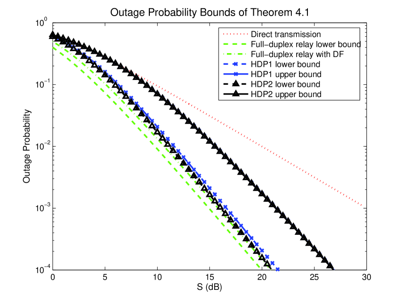
Figure 2: Outage probability bounds of Theorem IV.1.

The various bounds in this theorem are illustrated in Fig. 2.

For comparison purpose, it is easy to verify that the outage probability for direct transmission from the source to destination is $P_{\mathrm{dt}}(K,S)=\Pr(S\leq 1/Z_{13})=1-e^{\frac{1}{S}}\sim\mathcal{O}\left(\frac{1}{S}\right)$. From parts 1) and 6) of the theorem, we see that $\mathcal{O}\left(\frac{1}{S^{2}}\right)\leq P_{\mathrm{fd}}(K,S)\leq\mathcal{O}\left(\frac{1.5}{S^{2}}\right)$. Hence full-duplex relaying provides a second-order diversity outage performance as expected. In addition, when the rate requirement is small and the RNSNR is large, the loss in outage performance due to the restriction of half-duplex relaying is at most $0.9$dB by using HDP2. If phase synchronization between the source and relay is impractical, then employing HDP1 results in an additional loss of about $0.6$dB. Comparing parts 2) and 6), we see that HDP2 achieves the same outage performance as full-duplex relaying based on DF at asymptotically small rates. All these observations are readily illustrated in Fig. 2.

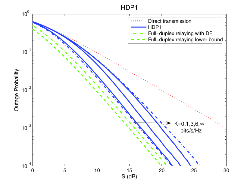
Figure 3: Outage probabilities for HDP1 obtained from Monte Carlo calculations.

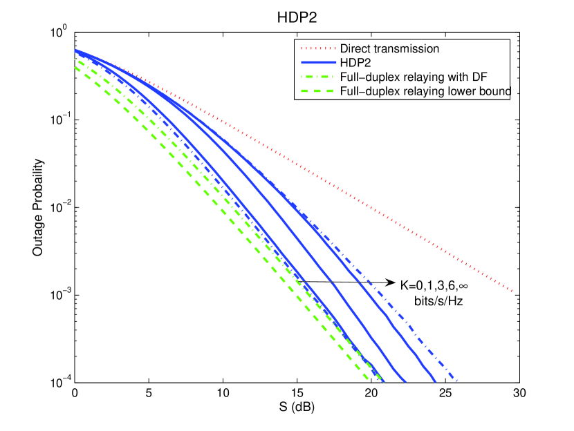
Figure 4: Outage probabilities for HDP2 obtained from Monte Carlo calculations.

When the rate requirement increases, the loss of half-duplex relaying starts to increase. In Figs. 3 and 4, we plot the outage probabilities achieved using HDP1 and HDP2, respectively. In each of the figures, we include the outage probabilities when the rate requirement approaches $0$, $1$, $3$, $6$, and $\infty$ bits/s/Hz. For comparison, we also plot the lower bounds on outage probabilities for full-duplex relaying in parts 1) and 2) of Theorem II.1 and the outage probability for direction transmission in the figures. All the results corresponding to HDP1 and HDP2 in the figures are obtained using Monte Carlo calculations. From Fig. 3, for HDP1, we see that the loss, with respect to full-duplex relaying at the outage probability of $10^{-4}$, is at most $1.5$dB at $1$ bits/s/Hz. The loss increases to about $2.7$dB and $4.2$dB when the rate increases to $3$ and $6$ bits/s/Hz, respectively. A similar trend is observed in Fig. 4 for HDP2. At $1$ bits/s/Hz, the loss is about $0.8$dB. The loss increases to $2.2$dB and $4.1$dB when the rate increases to $3$ and $6$ bits/s/Hz, respectively. Moreover, at all the values of $K$ considered for both HDP1 and HDP2, the simulation results seem to indicate that the outage probability is of the order of $\mathcal{O}\left(\frac{a}{S^{2}}\right)$ for some constant $a$, whose value is different for the different cases.

When the rate requirement becomes asymptotically large, Theorem IV.1 parts 3) and 5) state that the outage probabilities for HDP1 and HDP2 are at most of order $\mathcal{O}\left(\frac{4\log S}{S^{2}}\right)$. This implies that they both give close-to-second-order diversity performance at asymptotically high rates. From the simulation results shown in Figs. 3 and 4, it appears that the outage probabilities for both HDP1 and HDP2 do in fact have the order of $\mathcal{O}\left(\frac{a\log S}{S^{2}}\right)$, where $a$ is about $2.85$. This corresponds to a performance loss of about $5$dB at the outage probability of $10^{-4}$, and the bound in parts 3) and 5) is about $0.8$dB loose (cf. Fig. 2). We also note that HDP2 does not improve the outage performance, compared to HDP1, at asymptotically large rates. This is contrary to the finite rate cases in which HDP2 does provide performance advantage over HDP1, although the amount of advantage decreases as the rate requirement increases. In summary, HDP1 seems to be of higher practical utility than HDP2 since the former does not require phase synchronization between the source and relay, while it only suffers from a performance loss of about $0.6$dB.

IV-B $\varepsilon$-achievable rates

By using the standard sampling representation [22], the input-output relationship of the 3-node relay channel over a time slot can be written as

$$Y^{n} = \sqrt{Z_{13}}X_{1}^{n}+\sqrt{Z_{23}}X_{2}^{n}+N^{n}$$

$$Y_{1}^{n} = \sqrt{Z_{12}}X_{1}^{n}+N_{1}^{n},$$ (10)

where $X_{1}^{n}$, $X_{2}^{n}$, $Y^{n}$, $Y_{1}^{n}$, $N^{n}$, and $N_{1}^{n}$ are the $n$-element transmit symbol vector at the source, transmit symbol vector at the relay, receive symbol vector at the destination, receive symbol vector at the relay, Gaussian noise vector at the destination, and Gaussian noise vector at the relay, respectively. The dimension $n=2W$ and is assumed to be large. Conditioned on the link gain vector $Z=[Z_{13},Z_{12},Z_{23}]$, the channel is memoryless and described by the Gaussian conditional pdf $p_{Y^{n},Y_{1}^{n}|X_{1}^{n},X_{2}^{n},Z}(y^{n},y_{1}^{n}|x_{1}^{n},x_{2}^{n})$. An $(n,M_{n},\varepsilon_{n},P_{n})$-code [27] over a time slot is one that consists of the encoding and decoding functions described in [3] allowing one of $M_{n}$ messages to be sent from the source to destination in a time slot, and achieves the average (averaged over all codewords sent at the source and relay, link and noise realizations) error probability of $\varepsilon_{n}$, while the maximum (over all codewords) total transmit energy used in the time slot does not exceed $P_{n}$. Since the link gain vector is available at all nodes, we allow the transmit powers of the source and relay to vary as functions of the link gains. This corresponds to the application of power control [16]. As a result, the power control scheme is included implicitly in the code, and $P_{n}$ can be in general a function of the link gain vector $Z$. In most cases, we are interested in performing power control to minimize $\varepsilon_{n}$. The rate $K$ is $(\varepsilon,P_{t})$-achievable if there exists a sequence of $(n,M_{n},\varepsilon_{n},P_{n})$-codes satisfying $\limsup_{n\rightarrow\infty}\varepsilon_{n}\leq\varepsilon$, $\liminf_{n\rightarrow\infty}\frac{1}{n}\log M_{n}\geq K$, and $\limsup_{n\rightarrow\infty}P_{n}\leq P_{t}$ almost surely (a.s.).

For half-duplex relaying, when the relay listens (transmits), its transmit (receive) symbols are restricted to zero. In the previous sections, we have assumed that the relay first listens for $t_{1}$ seconds in a time slot and then transmits in the remaining $t_{2}$ seconds. In this case, it is more convenient to describe the channel by the CB and MA conditional pdfs, $p_{Y^{t_{1}n},Y_{1}^{t_{1}n}|X_{1}^{t_{1}n},Z}(y^{t_{1}n},y_{1}^{t_{1}n}|x_{1}^{t_{1}n})$ and $p_{Y^{t_{2}n}|X_{1}^{t_{2}n}X_{2}^{t_{2}n},Z}(y^{t_{2}n}|x_{1}^{t_{2}n},x_{2}^{t_{2}n})$, for the first and second sub-slots, respectively. We will also say that the rate $K$ is $(\varepsilon,P_{t})$-achievable with HDP1 (HDP2) if there exists a sequence of $(n,M_{n},\varepsilon_{n},P_{n})$-codes with the CB and MA coding in the first and second sub-slots as described in HDP1 (HDP2), satisfying $\limsup_{n\rightarrow\infty}\varepsilon_{n}\leq\varepsilon$, $\liminf_{n\rightarrow\infty}\frac{1}{n}\log M_{n}\geq K$, and $\limsup_{n\rightarrow\infty}P_{n}\leq P_{t}$ a.s.

The theorem below states that the various $\varepsilon$-achievable rates are characterized by the corresponding outage probabilities defined in the previous section.

Theorem IV.2

1. For all $\varepsilon>0$ and $0<\delta<1$, if the rate $K$ is $(\varepsilon,P_{t})$-achievable, then
   $\varepsilon\geq\delta P_{\mathrm{lb}}\left(K,\frac{e^{K}-1}{e^{(1-\delta)K}-1}S\right)$.

2. For all $\varepsilon>0$, the rate $K$ is $(\varepsilon,P_{t})$-achievable if $P_{\mathrm{DF}}(K,S)\leq\varepsilon$.

3. For all $\varepsilon>0$, the rate $K$ is $(\varepsilon,P_{t})$-achievable with HDP1 if $P_{1}(K,S)\leq\varepsilon$.

4. For all $\varepsilon>0$, the rate $K$ is $(\varepsilon,P_{t})$-achievable with HDP2 if $P_{2}(K,S)\leq\varepsilon$.

Proof:

See Appendix -G. ∎

IV-C Diversity-multiplexing tradeoff

It is also interesting to investigate the diversity-multiplexing tradeoff of [15] for HDP1 and HDP2. To this end, we need to follow [4] to change the parameterization of the outage probabilities from $(K,S)$ to $(\tilde{K},\tilde{S})$, where $\tilde{S}$ is the SNR and $\tilde{K}$ is the multiplexing gain ($0<\tilde{K}<1$) defined by

$$\tilde{K}=\frac{K}{\log(1+\tilde{S})}.$$

With the parameterization $(\tilde{K},\tilde{S})$, the diversity orders [15] achieved by HDP1 and HDP2 are defined as

$$\Delta_{i}(\tilde{K})=\lim_{\tilde{S}\rightarrow\infty}\frac{-\log P^{i}_{e}(\tilde{K},\tilde{S})}{\log\tilde{S}},$$

where $P^{i}_{e}(\tilde{K},\tilde{S})$ is the average error probability of HDP$i$ at SNR $\tilde{S}$ and multiplexing gain $\tilde{K}$, for $i=1$ and $2$, respectively. Then the diversity orders can be readily obtained in the following corollary of Theorems IV.1 and IV.2.

Corollary IV.1

For $i=1$ and $2$, $\Delta_{i}(\tilde{K})=2(1-\tilde{K})$. Hence HDP1 and HDP2 achieve the maximum diversity advantage possible for the relay channel when link gain information is available at all nodes.

Proof:

First, by Theorem IV.2, $P^{i}_{e}(\tilde{K},\tilde{S})\leq P_{i}(\tilde{K},\tilde{S})$ for $i=1$ and $2$. Also notice that since $\tilde{S}=S\left(e^{K}-1\right)$, $\displaystyle S=\frac{\tilde{S}}{(1+\tilde{S})^{\tilde{K}}-1}$. Hence $S\sim\mathcal{O}\left(\tilde{S}^{1-\tilde{K}}\right)$. As a result, applying parts 3) – 6) of Theorem IV.1 with the parameterization $(\tilde{K},\tilde{S})$, for sufficiently large $\tilde{S}$ and $i=1,2$,

$$\mathcal{O}\left(\frac{a_{i}}{\tilde{S}^{2(1-\tilde{K})}}\right)\leq P_{i}(\tilde{K},\tilde{S})\leq\mathcal{O}\left(\frac{4(1-\tilde{K})\log\tilde{S}}{\tilde{S}^{2(1-\tilde{K})}}\right),$$

where $a_{1}=2$ and $a_{2}=1.5$. Applying $-\log$, dividing the result by $\log\tilde{S}$, and finally taking limit as $\tilde{S}\rightarrow\infty$ on each item in the inequality equation above give $\Delta_{i}(\tilde{K})\geq 2(1-\tilde{K})$ for $i=1$ and $2$. On the other hand, part 1) of Theorem IV.1 and part 1) of Theorem IV.2 force the error probability of any transmission scheme over the relay channel to be larger than $\delta\mathcal{O}\left(\frac{e^{1-\delta}}{\tilde{S}^{2(1-\tilde{K})}}\right)$ for all $0<\delta<1$. As a result, the maximum possible diversity order of any transmission scheme over the relay channel is $2(1-\tilde{K})$. Thus we have the desired result. ∎

IV-D Delay-limited rates

When the average error probability decreases to zero, the $\varepsilon$-achievable rates becomes the delay-limited rates [16]. We calculate the delay-limited rates achievable by HDP1 and HDP2 in this section.

We first employ the following definition [27] as our definition of delay limited rate: The rate $K$ is $P_{t}$-achievable if there exists a sequence of $(n,M_{n},\varepsilon_{n},P_{n})$-codes over a time slot, satisfying $\lim_{n\rightarrow\infty}\varepsilon_{n}=0$, $\liminf_{n\rightarrow\infty}\frac{1}{n}\log M_{n}\geq K$, and $\limsup_{n\rightarrow\infty}P_{n}\leq P_{t}$ a.s. . Unfortunately, part 1) of Theorem IV.2 forces the $P_{t}$-achievable rate of any transmission scheme over the relay channel to be zero as long as $P_{t}$ is finite. This is due to the Rayleigh fading nature of the links and the restriction that the total transmit energy in each time slot needs to be bounded by $P_{t}$. It turns out that more meaningful results can be obtained if we relax the latter restriction.

Recall that the link power gains vary independently from time slot to time slot. With power control to maintain the error probability $\varepsilon_{n}$, the total transmit energy $P_{n}$ (a function of $Z$) of an $(n,M_{n},\varepsilon_{n},P_{n})$-code may vary from time slot to time slot. This may require the total transmit energy to be very large in the worst faded time slots. As a relaxation of the transmit energy constraint, we require the average total transmit energy per time slot over many time slots to be bounded. Then the ergodicity of the fading process requires $E[P_{n}]$ to be bounded. This relaxation motivates the following definition: The rate $K$ is long-term $P_{t}$-achievable if there exists a sequence of $(n,M_{n},\varepsilon_{n},P_{n})$-codes over a time slot, satisfying $\lim_{n\rightarrow\infty}\varepsilon_{n}=0$, $\liminf_{n\rightarrow\infty}\frac{1}{n}\log M_{n}\geq K$, and $\limsup_{n\rightarrow\infty}E[P_{n}]\leq P_{t}$.

The following theorem then specifies the delay-limited rates achievable by HDP1 and HDP2:

Theorem IV.3

For $K>0$, define

$$P^{\mathrm{lb}}_{t}(K) = E[B_{\mathrm{lb}}](e^{K}-1)N_{0}W$$

$$P^{\mathrm{DF}}_{t}(K) = E[B_{\mathrm{DF}}](e^{K}-1)N_{0}W$$

$$P^{1}_{t}(K) = E[B_{1}(K)](e^{K}-1)N_{0}W$$

$$P^{2}_{t}(K) = E[B_{2}(K)](e^{K}-1)N_{0}W.$$

Then $P^{\mathrm{lb}}_{t}(K)\leq P^{\mathrm{DF}}_{t}(K)\leq P^{2}_{t}(K)\leq P^{1}_{t}(K)<\infty$.

1. If the rate $K$ is long-term $P_{t}$-achievable, then $P_{t}\geq P^{\mathrm{lb}}_{t}(K)$.

2. The rate $K$ is long-term $P^{\mathrm{DF}}_{t}(K)$-achievable.

3. The rate $K$ is long-term $P^{1}_{t}(K)$-achievable with HDP1.

4. The rate $K$ is long-term $P^{2}_{t}(K)$-achievable with HDP2.

Proof:

See Appendix -H. ∎

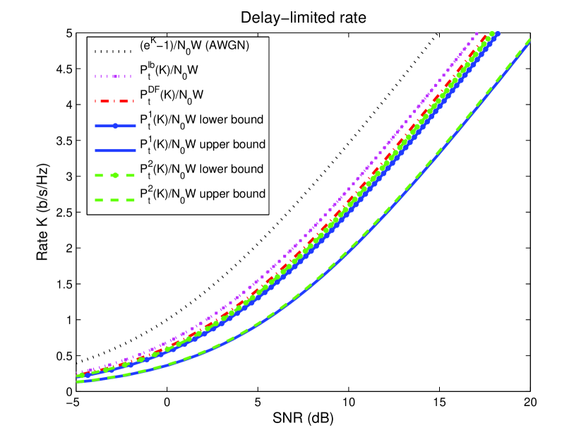
Figure 5: Plot of delayed-limited rates for various transmission schemes.

In Fig. 5, we plot the rate $K$ against $\frac{P_{t}^{i}(K)}{N_{0}W}$ for $i\in\{\mathrm{lb},\mathrm{DF}\}$. For $i\in\{1,2\}$, notice that

$$E[B_{i}(0)](e^{K}-1)\leq\frac{P_{t}^{i}(K)}{N_{0}W}\leq E[B_{i}(\infty)](e^{K}-1)$$

by Corollaries III.1 and III.2, respectively. In each case, we plot the lower and upper bounds instead. The true $\frac{P_{t}^{i}(K)}{N_{0}W}$ curve lies between the bounding curves. Also the true curve approaches the lower bound when $K$ is small and the upper bound when $K$ is large. For comparison, we also plot the curve $\frac{e^{K}-1}{N_{0}W}$ which corresponds to the SNR required to achieve the rate $K$ in an additive white Gaussian noise (AWGN) channel with unit power gain. Thus, at each rate, the loss of performance, with respect to an AWGN channel, in dB for approach $i$ due to link fading and the restriction of one-slot decoding delay is $E[B_{i}]_{\mathrm{dB}}=10\log_{10}(E[B_{i}])$. The results obtained from numerical calculations are shown in Table I. From the table, we see that the loss when employing full-duplex relaying is between $2.17$dB and $2.76$dB, where the upper limit on the loss can be achieved by DF with optimal power control. The loss when using HDP1 with optimal power control ranges from $3.33$dB to $5.45$dB, while the loss when using HDP2 with optimal power control is between $3.02$dB and $5.36$dB. The loss of performance of half-duplex relaying with respect to full-duplex relaying is at most $3.28$dB. This loss happens when the rate requirement is very large and HDP1 is employed. When the rate is very small, the loss drops down to at most $0.85$dB with the use of HDP2. With the delay-limited rate as performance measure, HDP1 once again appears to be a good tradeoff between complexity and performance. The maximum loss when using HDP1 instead of HDP2 is only $0.31$dB.

V Conclusions

With channel state information available at all nodes, we have shown that a half-duplex cooperative transmission design, based on optimizing distinct flows through the direct link from the source to the destination and the path via the relay, can effectively harness diversity advantage of the relay channel in both high-rate and low-rate scenarios. Specifically, the proposed design gives outage performance approaching that of full-duplex relaying using decode-and-forward at asymptotically low rates. When the rate requirement becomes asymptotically large, the design still gives a close-to-second-order outage diversity performance. The design also gives the best diversity-multiplexing tradeoff possible for the relay channel. With optimal long-term power control over the fading relay channel, the proposed design can give delay-limited rate performance that is within a few dBs of the capacity performance of the additive white Gaussian channel in both low-rate and high-rate scenarios.

In addition to the good performance, a perhaps more important advantage of the proposed relaying design is that only flow-level design is needed to optimize the use of the rather standard components of cooperative broadcasting and multiple access. This advantage makes generalizations of the design to more-complicated relay networks manageable. In general, the availability of channel information at the nodes appears to simplify cooperative transmission designs. Thus it is worthwhile to investigate how to effectively spread the channel state information in a wireless network.

-A Proof of Theorem II.1

First consider the sufficient condition in Theorem II.1. We consider two different cases:

-A1 $Z_{12}>Z_{13}$

Let $0\leq\alpha\leq 1$ be the fraction of the total energy, $P_{t}$, allocated to the source node. Then the transmit energy of the relay node is $(1-\alpha)P_{t}$. By [3, Theorem 1] (also see [5]), the following rate is achievable by the relay channel when the relay decodes and re-encodes its received signal:

$$R_{\textrm{DF}}(\alpha) = \max_{0\leq\beta\leq 1}\min\left\{C\left(\frac{P_{t}}{N_{0}W}\left[\alpha Z_{13}+(1-\alpha)Z_{23}+2\sqrt{(1-\beta)\alpha(1-\alpha)Z_{13}Z_{23}}\right]\right),\right.$$ (11)

$$~{}~{}~{}~{}~{}~{}~{}~{}~{}~{}~{}~{}~{}~{}~{}\left.C\left(\frac{P_{t}}{N_{0}W}\alpha\beta Z_{12}\right)\right\},$$

where $C(x)=\log(1+x)$. We can further maximize the rate by optimally allocating transmit energy between the source and relay, i.e.,

$$R_{\textrm{DF}} = \max_{0\leq\alpha\leq 1}R_{\textrm{DF}}(\alpha)$$

$$= C\left(\frac{P_{t}}{N_{0}W}\max_{0\leq\alpha,\beta\leq 1}\min\left\{\alpha Z_{13}+(1-\alpha)Z_{23}+2\sqrt{(1-\beta)\alpha(1-\alpha)Z_{13}Z_{23}},\alpha\beta Z_{12}\right\}\right),$$

where the second equality results from the fact that $C(x)$ is an increasing function. Hence, the requirement that the RNSNR satisfies $S>1/Z_{\textrm{DF}}$ is sufficient for $R_{\textrm{DF}}=K$, where

$$Z_{\textrm{DF}}=\max_{0\leq\alpha,\beta\leq 1}\min\left\{\alpha Z_{13}+(1-\alpha)Z_{23}+2\sqrt{(1-\beta)\alpha(1-\alpha)Z_{13}Z_{23}},\alpha\beta Z_{12}\right\}.$$ (12)

Thus it reduces to solving the optimization problem in (12).

To solve (12), we write $\displaystyle Z_{\textrm{DF}}(\alpha)=\max_{0\leq\beta\leq 1}\min\left\{\alpha Z_{13}+(1-\alpha)Z_{23}+2\sqrt{(1-\beta)\alpha(1-\alpha)Z_{13}Z_{23}},\alpha\beta Z_{12}\right\}.$ and consider two cases:

$\displaystyle 0\leq\alpha\leq\frac{Z_{23}}{Z_{23}+Z_{12}-Z_{13}}$

Under this case, the second term inside the $\min$ operator is smaller than the first term for all $0\leq\beta\leq 1$. Hence $Z_{\textrm{DF}}(\alpha)=\max_{0\leq\beta\leq 1}\alpha\beta Z_{12}=\alpha Z_{12}$.

$\displaystyle\frac{Z_{23}}{Z_{23}+Z_{12}-Z_{13}}<\alpha\leq 1$

Under this case, notice that the first and second terms inside the $\min$ operator are strictly decreasing and increasing in $\beta$, respectively. Moreover the two terms equalize at some $0\leq\beta_{*}\leq 1$. Hence $Z_{\textrm{DF}}(\alpha)=\alpha\beta_{*}Z_{12}$. Solving for the equalizing $\beta_{*}$, we get

$$Z_{\textrm{DF}}(\alpha)=\alpha Z_{13}+(1-\alpha)Z_{23}\left(1-2\frac{Z_{13}}{Z_{12}}\right)+2\sqrt{(1-\alpha)\frac{Z_{13}}{Z_{12}}\left(1-\frac{Z_{13}}{Z_{12}}\right)Z_{23}\left[\alpha Z_{12}-(1-\alpha)Z_{23}\right]}.$$

Now we maximize $Z_{\textrm{DF}}(\alpha)$ over $0\leq\alpha\leq 1$. For case a), $\displaystyle\max_{\alpha}Z_{\textrm{DF}}(\alpha)=\frac{Z_{12}Z_{23}}{Z_{23}+Z_{12}-Z_{13}}$. For case b), a direct but tedious calculation shows that $\displaystyle\max_{\alpha}Z_{\textrm{DF}}(\alpha)=\frac{Z_{12}(Z_{13}+Z_{23})}{Z_{12}+Z_{23}}$. It is not hard to verify that the maximum value in case b) is larger than the maximum value in case a). Hence $\displaystyle Z_{\textrm{DF}}=\frac{Z_{12}(Z_{13}+Z_{23})}{Z_{12}+Z_{23}}$, and the sufficient condition is $\displaystyle S>\frac{Z_{12}+Z_{23}}{Z_{12}(Z_{13}+Z_{23})}$.

-A2 $Z_{12}\leq Z_{13}$

First note that the capacity of the relay channel is upper bounded by the maximum sum rate of the CB channel from the source to the relay and destination. This CB channel is a degraded Gaussian broadcast channel, and the individual rates $R_{13}$ and $R_{12}$ from the source to the destination and relay, respectively, satisfy [22, Ch. 14]

$$R_{13} < C\left(\frac{\alpha Z_{13}P_{t}}{N_{0}W}\right)$$

$$R_{12} < C\left(\frac{(1-\alpha)Z_{12}P_{t}}{\alpha Z_{12}P_{t}+N_{0}W}\right),$$ (13)

for any $0\leq\alpha\leq 1$. To have $R_{13}+R_{12}\geq K$, we need

$$K < \max_{0\leq\alpha\leq 1}\left\{C\left(\frac{\alpha Z_{13}P_{t}}{N_{0}W}\right)+C\left(\frac{(1-\alpha)Z_{12}P_{t}}{\alpha Z_{12}P_{t}+N_{0}W}\right)\right\}$$

$$= \log\left[\left(1+Z_{12}\frac{P_{t}}{N_{0}W}\right)\cdot\max_{0\leq\alpha\leq 1}\left(\frac{1+\alpha Z_{13}\frac{P_{t}}{N_{0}W}}{1+\alpha Z_{12}\frac{P_{t}}{N_{0}W}}\right)\right]$$

$$= C\left(Z_{13}\frac{P_{t}}{N_{0}W}\right),$$

where the last equality is obtained by choosing $\alpha=1$, due to the condition that $Z_{13}\geq Z_{12}$. Hence $S>1/Z_{13}$. This lower bound corresponds to sending all information directly form the source to the destination without using the relay.

For the necessary condition, we employ the max-flow-min-cut bound of [22, Theorem 14.10.1] to obtain an upper bound, $R_{\textrm{lb}}(\alpha)$, on the rate of the relay channel. It turns out [5] that the expression for $R_{\textrm{lb}}(\alpha)$ is obtained simply by replacing every occurrence of $Z_{12}$ by $Z_{12}+Z_{13}$ in (11) above. In addition, the power optimization procedure in case 1) above carries through directly for this case with every occurrence of $Z_{12}$ replaced by $Z_{12}+Z_{13}$. Thus we obtain the necessary condition as $\displaystyle S\geq\frac{Z_{12}+Z_{13}+Z_{23}}{(Z_{12}+Z_{13})(Z_{13}+Z_{23})}$.

-B Proof of Lemma III.1

1. The case of $t_{1}=0$ trivially requires $x_{1}=x_{2}=0$, and hence $S_{\textrm{CB}}=0$. So we consider $0<t_{1}\leq 1$. If $Z_{13}>Z_{12}$, we have a degraded broadcast channel during this time slot. Thus rate constraints in (13) must be satisfied with $R_{13}=x_{1}/t_{1}$ and $R_{12}=x_{2}/t_{1}$. Combining the two inequalities to remove $\alpha$, it is easy to obtain the stated lower bound $S_{\textrm{CB}}$ of the SNR $P_{t}/N_{0}W$. We note that this lower bound corresponds to the optimal choice $\alpha=\frac{\displaystyle(e^{x_{1}/t_{1}}-1)/{Z_{13}}}{\displaystyle(e^{x_{2}/t_{1}}-1)/Z_{12}+e^{x_{2}/t_{1}}(e^{x_{1}/t_{1}}-1)/Z_{13}}$. Interchanging the roles of $Z_{13}$ and $Z_{12}$, we get the stated SNR lower bound for the case of $Z_{13}\leq Z_{12}$.

2. The case of $t_{2}=0$ trivially requires $x_{2}=x_{3}=0$, and hence $S_{\textrm{MA}}=0$. So we consider $0<t_{2}\leq 1$. The capacity region of this Gaussian MA channel is specified by [22, Ch. 14]:

   $$\frac{x_{3}}{t_{2}} < C\left(\frac{\alpha Z_{13}P_{t}}{N_{0}W}\right),$$

   $$\frac{x_{2}}{t_{2}} < C\left(\frac{(1-\alpha)Z_{23}P_{t}}{N_{0}W}\right),$$

   $$\frac{x_{2}+x_{3}}{t_{2}} < C\left(\frac{[\alpha Z_{13}+(1-\alpha)Z_{23}]P_{t}}{N_{0}W}\right),$$ (14)

   for any $0\leq\alpha\leq 1$, where $\alpha$ and $1-\alpha$ are the fractions of the transmit power assigned to the source and relay, respectively. We want to optimally choose $\alpha$ so that the SNR $P_{t}/N_{0}W$ required to satisfy (14) is minimized. First, suppose that $Z_{13}>Z_{23}$. Then rearranging the second and third inequalities in (14) gives

   $$\alpha < 1-\frac{1}{Z_{23}}\left(e^{x_{2}/t_{2}}-1\right)\frac{N_{0}W}{P_{t}},$$

   $$\alpha > \frac{1}{Z_{13}-Z_{23}}\cdot\left\{\left[e^{(x_{2}+x_{3})/t_{2}}-1\right]\frac{N_{0}W}{P_{t}}-Z_{23}\right\},$$

   respectively. Combining these two inequalities to remove $\alpha$, we obtain the stated lower bound $S_{\textrm{MA}}$. We note that the corresponding optimal choice $\alpha=\frac{\displaystyle(e^{x_{3}/t_{2}}-1)/{Z_{13}}}{\displaystyle(e^{x_{2}/t_{2}}-1)/Z_{23}+e^{x_{2}/t_{2}}(e^{x_{3}/t_{2}}-1)/Z_{13}}$.

   Interchanging the roles of $Z_{13}$ and $Z_{23}$, we get the stated SNR lower bound for the case of $Z_{13}<Z_{23}$. When $Z_{13}=Z_{23}$, the third inequality in (14) gives the stated lower bound $S_{\textrm{MA}}$. The choice of optimal $\alpha$ in this case is exactly the same as the one in the case of $Z_{13}>Z_{23}$ (or $Z_{13}<Z_{23}$).

-C Solution to optimization problem (1)

Suppose that $t_{1}$ and $t_{2}$ are fixed, satisfying both the non-negativity and total-time requirements. Then we can view the optimization problem (1) as a convex optimization problem in $x_{1}$, $x_{2}$ and $x_{3}$. Rewriting it in standard form [23]:

$$\begin{array}[]{lll}&\displaystyle\min_{x_{1},x_{2},x_{3}}\tilde{S}(t_{1},t_{2})=t_{1}S_{\mathrm{CB}}+t_{2}S_{\mathrm{MA}}&\\ \mbox{Subject to}&\mbox{i. total-data requirement:}&x_{1}+x_{2}+x_{3}=K\\ &\mbox{ii. non-negativity requirements:}&-x_{1},-x_{2},-x_{3}\leq 0\end{array}$$ (15)

Since this optimization problem is convex, the rate tuple $(x_{1},x_{2},x_{3})$ is a solution if it satisfies the following KKT conditions:

1. $\displaystyle\nabla\tilde{S}+\sum_{i=1}^{3}\lambda_{i}\nabla(-x_{i})+\mu\nabla(x_{1}+x_{2}+x_{3}-K)=0$

2. $\lambda_{i}(-x_{i})=0$ for $i=1,2,3$

3. $\lambda_{i}\geq 0$ for $i=1,2,3$

4. $-x_{i}\leq 0$ for $i=1,2,3$

5. $x_{1}+x_{2}+x_{3}=K$.

Our approach to solve the original optimization problem (1) is to first solve the sub-problem (15) for each pair of $(t_{1},t_{2})$, and then minimize $\min_{x_{1},x_{2},x_{3}}\tilde{S}(t_{1},t_{2})$ over all allowable pairs. To this end, we consider the following cases and obtain solution to the optimization problem (15) by directly checking the KKT conditions. Note that we assume in below that both $t_{1}$ and $t_{2}$ are positive. For $t_{2}=0$ ($t_{1}=0$), Lemma III.1 tells us that the transmission in the first (second) sub-slots reduces trivially to transmission over the direct link from the source to the destination. Hence $\min_{x_{1},x_{2},x_{3}}\tilde{S}(1,0)=\min_{x_{1},x_{2},x_{3}}\tilde{S}(0,1)=\left(e^{K}-1\right)/Z_{13}$.

-C1 $Z_{13}\geq Z_{12}$ and $Z_{13}\geq Z_{23}$

From Lemma III.1,

$$\tilde{S}(t_{1},t_{2})=\frac{t_{1}}{Z_{12}}\left(e^{x_{2}/t_{1}}-1\right)+\frac{t_{1}}{Z_{13}}e^{x_{2}/t_{1}}\left(e^{x_{1}/t_{1}}-1\right)+\frac{t_{2}}{Z_{23}}\left(e^{x_{2}/t_{2}}-1\right)+\frac{t_{2}}{Z_{13}}e^{x_{2}/t_{2}}\left(e^{x_{3}/t_{2}}-1\right).$$

The condition K1 yields

$$\begin{array}[]{l}\displaystyle\frac{1}{Z_{13}}e^{(x_{1}+x_{2})/t_{1}}-\lambda_{1}+\mu=0\\ \displaystyle\frac{1}{Z_{12}}e^{x_{2}/t_{1}}+\frac{1}{Z_{13}}e^{x_{2}/t_{1}}(e^{x_{1}/t_{1}}-1)+\frac{1}{Z_{23}}e^{x_{2}/t_{2}}+\frac{1}{Z_{13}}e^{x_{2}/t_{2}}(e^{x_{3}/t_{2}}-1)-\lambda_{2}+\mu=0\\ \displaystyle\frac{1}{Z_{13}}e^{(x_{2}+x_{3})/t_{2}}-\lambda_{3}+\mu=0.\end{array}$$

It is then easy to check that the following solution satisfy the KKT conditions:

$$\begin{array}[]{ll}x_{1}=Kt_{1},&\lambda_{1}=0\\ \displaystyle x_{2}=0,&\displaystyle\lambda_{2}=\frac{1}{Z_{12}}+\frac{1}{Z_{23}}-\frac{1}{Z_{13}}+\frac{1}{Z_{13}}(e^{K}-1)\\ x_{3}=Kt_{2},&\lambda_{3}=0\\ \displaystyle\mu=-\frac{1}{Z_{13}}e^{K}.\end{array}$$

-C2 $Z_{13}\geq Z_{12}$ and $Z_{13}<Z_{23}$

From Lemma III.1,

$$\tilde{S}(t_{1},t_{2})=\frac{t_{1}}{Z_{12}}\left(e^{x_{2}/t_{1}}-1\right)+\frac{t_{1}}{Z_{13}}e^{x_{2}/t_{1}}\left(e^{x_{1}/t_{1}}-1\right)+\frac{t_{2}}{Z_{13}}\left(e^{x_{3}/t_{2}}-1\right)+\frac{t_{2}}{Z_{23}}e^{x_{3}/t_{2}}\left(e^{x_{2}/t_{2}}-1\right).$$

The condition K1 yields

$$\begin{array}[]{l}\displaystyle\frac{1}{Z_{13}}e^{(x_{1}+x_{2})/t_{1}}-\lambda_{1}+\mu=0\\ \displaystyle\frac{1}{Z_{12}}e^{x_{2}/t_{1}}+\frac{1}{Z_{13}}e^{x_{2}/t_{1}}(e^{x_{1}/t_{1}}-1)+\frac{1}{Z_{23}}e^{(x_{2}+x_{3})/t_{2}}-\lambda_{2}+\mu=0\\ \displaystyle\frac{1}{Z_{13}}e^{x_{3}/t_{2}}+\frac{1}{Z_{23}}e^{x_{3}/t_{2}}(e^{x_{2}/t_{2}}-1)-\lambda_{3}+\mu=0.\end{array}$$

It is then easy to check that the following solution satisfy the KKT conditions:

$$\begin{array}[]{ll}x_{1}=Kt_{1},&\lambda_{1}=0\\ \displaystyle x_{2}=0,&\displaystyle\lambda_{2}=\frac{1}{Z_{12}}-\frac{1}{Z_{13}}+\frac{1}{Z_{23}}e^{K}\\ x_{3}=Kt_{2},&\lambda_{3}=0\\ \displaystyle\mu=-\frac{1}{Z_{13}}e^{K}.\end{array}$$

-C3 $Z_{13}<Z_{12}$ and $Z_{13}\geq Z_{23}$

From Lemma III.1,

$$\tilde{S}(t_{1},t_{2})=\frac{t_{1}}{Z_{13}}\left(e^{x_{1}/t_{1}}-1\right)+\frac{t_{1}}{Z_{12}}e^{x_{1}/t_{1}}\left(e^{x_{2}/t_{1}}-1\right)+\frac{t_{2}}{Z_{23}}\left(e^{x_{2}/t_{2}}-1\right)+\frac{t_{2}}{Z_{13}}e^{x_{2}/t_{2}}\left(e^{x_{3}/t_{2}}-1\right).$$

The condition K1 yields

$$\begin{array}[]{l}\displaystyle\frac{1}{Z_{13}}e^{x_{1}/t_{1}}+\frac{1}{Z_{12}}e^{x_{1}/t_{1}}(e^{x_{2}/t_{1}}-1)-\lambda_{1}+\mu=0\\ \displaystyle\frac{1}{Z_{12}}e^{(x_{1}+x_{2})/t_{1}}+\frac{1}{Z_{23}}e^{x_{2}/t_{2}}+\frac{1}{Z_{13}}e^{x_{2}/t_{2}}(e^{x_{3}/t_{2}}-1)-\lambda_{2}+\mu=0\\ \displaystyle\frac{1}{Z_{13}}e^{(x_{2}+x_{3})/t_{2}}-\lambda_{3}+\mu=0.\end{array}$$

It is then easy to check that the following solution satisfy the KKT conditions:

$$\begin{array}[]{ll}x_{1}=Kt_{1},&\lambda_{1}=0\\ x_{2}=0,&\displaystyle\lambda_{2}=\frac{1}{Z_{12}}e^{K}+\frac{1}{Z_{23}}-\frac{1}{Z_{13}}\\ x_{3}=Kt_{2},&\lambda_{3}=0\\ \displaystyle\mu=-\frac{1}{Z_{13}}e^{K}.\end{array}$$

-C4 $M_{H}(Z_{12},Z_{23})\leq Z_{13}<\min\{Z_{12},Z_{23}\}$

From Lemma III.1,

$$\tilde{S}(t_{1},t_{2})=\frac{t_{1}}{Z_{13}}\left(e^{x_{1}/t_{1}}-1\right)+\frac{t_{1}}{Z_{12}}e^{x_{1}/t_{1}}\left(e^{x_{2}/t_{1}}-1\right)+\frac{t_{2}}{Z_{13}}\left(e^{x_{3}/t_{2}}-1\right)+\frac{t_{2}}{Z_{23}}e^{x_{3}/t_{2}}\left(e^{x_{2}/t_{2}}-1\right).$$

The condition K1 yields

$$\begin{array}[]{l}\displaystyle\frac{1}{Z_{13}}e^{x_{1}/t_{1}}+\frac{1}{Z_{12}}e^{x_{1}/t_{1}}(e^{x_{2}/t_{1}}-1)-\lambda_{1}+\mu=0\\ \displaystyle\frac{1}{Z_{12}}e^{(x_{1}+x_{2})/t_{1}}+\frac{1}{Z_{23}}e^{(x_{2}+x_{3})/t_{2}}-\lambda_{2}+\mu=0\\ \displaystyle\frac{1}{Z_{13}}e^{x_{3}/t_{2}}+\frac{1}{Z_{23}}e^{x_{3}/t_{2}}(e^{x_{2}/t_{2}}-1)-\lambda_{3}+\mu=0.\end{array}$$

It is then easy to check that the following solution satisfy the KKT conditions:

$$\begin{array}[]{ll}x_{1}=Kt_{1},&\lambda_{1}=0\\ x_{2}=0,&\displaystyle\lambda_{2}=(\frac{1}{Z_{12}}+\frac{1}{Z_{23}}-\frac{1}{Z_{13}})e^{K}\\ x_{3}=Kt_{2},&\lambda_{3}=0\\ \displaystyle\mu=-\frac{1}{Z_{13}}e^{K}.\end{array}$$

-C5 ${Z_{13}}<M_{H}({Z_{12}},{Z_{23}})$

The expression for $\tilde{S}(t_{1},t_{2})$ in case 4) still holds. However, we need to consider the following two sub-cases in order to express the solution to the optimization problem (15):

$K>M_{H}(\log A_{1},\log A_{2})$

1. For $1-\frac{K}{\log A_{1}}\leq t_{1}\leq\frac{K}{\log A_{2}}$, the following solution satisfies the KKT conditions:

   $$\begin{array}[]{ll}x_{1}=Kt_{1}-t_{1}t_{2}\log A_{1},&\lambda_{1}=0\\ x_{2}=t_{1}t_{2}\log(A_{1}A_{2}),&\lambda_{2}=0\\ x_{3}=Kt_{2}-t_{1}t_{2}\log A_{2},&\lambda_{3}=0\\ \displaystyle\mu=-\frac{1}{Z_{12}}e^{K+t_{2}\log A_{2}}-\frac{1}{Z_{23}}e^{K+t_{1}\log A_{1}}.\end{array}$$

2. For $\frac{K}{\log A_{2}}<t_{1}<1$, the following solution satisfies the KKT conditions:

   $$\begin{array}[]{ll}x_{1}=Kt_{1}-t_{1}t_{2}\log A_{1},&\lambda_{1}=0\\ x_{2}=Kt_{2}+t_{1}t_{2}\log A_{1},&\lambda_{2}=0\\ x_{3}=0,&\displaystyle\lambda_{3}=\frac{1}{Z_{13}}-\frac{1}{Z_{23}}-\frac{1}{Z_{12}}e^{K/t_{1}}\\ \displaystyle\mu=-\frac{1}{Z_{23}}e^{K+t_{1}\log A_{1}}-\frac{1}{Z_{12}}e^{K/t_{1}}.\end{array}$$

3. For $0<t_{1}<1-\frac{K}{\log A_{1}}$, the following solution satisfies the KKT conditions:

   $$\begin{array}[]{ll}x_{1}=0,&\displaystyle\lambda_{1}=\frac{1}{Z_{13}}-\frac{1}{Z_{12}}-\frac{1}{Z_{23}}e^{K/t_{2}}\\ x_{2}=Kt_{1}+t_{1}t_{2}\log A_{2},&\lambda_{2}=0\\ x_{3}=Kt_{2}-t_{1}t_{2}\log A_{2},&\lambda_{3}=0\\ \displaystyle\mu=-\frac{1}{Z_{12}}e^{K+t_{2}\log A_{2}}-\frac{1}{Z_{23}}e^{K/t_{2}}.\end{array}$$

$K\leq M_{H}(\log A_{1},\log A_{2})$

1. For $\frac{K}{\log A_{2}}\leq t_{1}\leq 1-\frac{K}{\log A_{1}}$, the following solution satisfies the KKT conditions:

   $$\begin{array}[]{ll}x_{1}=0,&\displaystyle\lambda_{1}=\frac{1}{Z_{13}}-\frac{1}{Z_{12}}-\frac{1}{Z_{23}}e^{K/t_{2}}\\ x_{2}=K,&\lambda_{2}=0\\ x_{3}=0,&\displaystyle\lambda_{3}=\frac{1}{Z_{13}}-\frac{1}{Z_{23}}-\frac{1}{Z_{12}}e^{K/t_{1}}\\ \displaystyle\mu=-\frac{1}{Z_{12}}e^{K/t_{1}}-\frac{1}{Z_{23}}e^{K/t_{2}}.\end{array}$$

2. For $1-\frac{K}{\log A_{1}}<t_{1}<1$, the following solution satisfies the KKT conditions:

   $$\begin{array}[]{ll}x_{1}=Kt_{1}-t_{1}t_{2}\log A_{1},&\lambda_{1}=0\\ x_{2}=Kt_{2}+t_{1}t_{2}\log A_{1},&\lambda_{2}=0\\ x_{3}=0,&\displaystyle\lambda_{3}=\frac{1}{Z_{13}}-\frac{1}{Z_{23}}-\frac{1}{Z_{12}}e^{K/t_{1}}\\ \displaystyle\mu=-\frac{1}{Z_{23}}e^{K+t_{1}\log A_{1}}-\frac{1}{Z_{12}}e^{K/t_{1}}.\end{array}$$

3. For $0<t_{1}<\frac{K}{\log A_{2}}$, the following solution satisfies the KKT conditions:

   $$\begin{array}[]{ll}x_{1}=0,&\displaystyle\lambda_{1}=\frac{1}{Z_{13}}-\frac{1}{Z_{12}}-\frac{1}{Z_{23}}e^{K/t_{2}}\\ x_{2}=Kt_{1}+t_{1}t_{2}\log A_{2},&\lambda_{2}=0\\ x_{3}=Kt_{2}-t_{1}t_{2}\log A_{2},&\lambda_{3}=0\\ \displaystyle\mu=-\frac{1}{Z_{12}}e^{K+t_{2}\log A_{2}}-\frac{1}{Z_{23}}e^{K/t_{2}}.\end{array}$$

For cases 1)–4), direction substitution of the solution yields $\min_{x_{1},x_{2},x_{3}}\tilde{S}(t_{1},t_{2})=\left(e^{K}-1\right)/Z_{13}$. Since this solution is independent of the choice of $(t_{1},t_{2})$, the solution to the optimization problem (1) in these four cases is simply $\left(e^{K}-1\right)/Z_{13}$. Also note that these four cases can be collectively specified by the condition $Z_{13}\geq M_{H}(Z_{12},Z_{23})$.

For case 5a), the three functions $\tilde{S}_{1}(K)$, $\tilde{S}_{2}(K)$, and $\tilde{S}_{3}(K)$ respectively described in (3), (4), and (5) can be obtained by direct substitution of the solutions in the 3 sub-cases (i., ii., and iii, respectively), and then minimizing the corresponding $\min_{x_{1},x_{2},x_{3}}\tilde{S}(t_{1},t_{2})$ over the range of $t_{1}$ specified in each sub-cases. Hence the final solution of the optimization problem (1) is obtained by finding the minimum among the these three functions. For case 5b), a similar procedure yields the fact that the solution to the optimization problem (1) is the minimum among the three functions $\hat{S}_{1}(K)$, $\hat{S}_{2}(K)$, and $\hat{S}_{3}(K)$ respectively described in (7), (8), and (9).

-D Proof of Corollary III.1

The proof of the results in this corollary is based on the fact that $B_{1}(K)$ is the (normalized) solution to the optimization problem (1) and the form of $B_{1}(K)$ described in Section III-A1.

1. Fix $Z_{13}$, $Z_{12}$, and $Z_{23}$. From the description of $B_{1}(K)$ in Section III-A1, since $B_{1}(K)$ is trivially continuous and non-decreasing in $K$ when under the condition $Z_{13}\geq M_{H}(Z_{12},Z_{23})$, it suffices to consider $B_{1}(K)$ under the condition $Z_{13}<M_{H}(Z_{12},Z_{23})$, which is assumed for the rest of the proof.

   For convenience, let us denote the respective functions inside the $\min$ operators of $\tilde{S}_{1}(K)$, $\tilde{S}_{2}(K)$, $\tilde{S}_{3}(K)$, $\hat{S}_{1}(K)$, $\hat{S}_{2}(K)$, and $\hat{S}_{3}(K)$ by the addition of the sign ^′. Define, for $0\leq t_{1}\leq 1$,

   $$\tilde{B}(K,t_{1})=\left\{\begin{array}[]{ll}\frac{\tilde{S}_{1}^{\prime}(K)}{e^{K}-1}&\mbox{~{}if~{}}K>M_{H}(\log A_{1},\log A_{2})\mbox{~{}and~{}}\max\left\{0,1-\frac{K}{\log A_{1}}\right\}\leq t_{1}\leq\min\left\{\frac{K}{\log A_{2}},1\right\}\\ \frac{\tilde{S}_{2}^{\prime}(K)}{e^{K}-1}&\mbox{~{}if~{}}K>M_{H}(\log A_{1},\log A_{2})\mbox{~{}and~{}}\min\left\{\frac{K}{\log A_{2}},1\right\}\leq t_{1}\leq 1\\ \frac{\tilde{S}_{3}^{\prime}(K)}{e^{K}-1}&\mbox{~{}if~{}}K>M_{H}(\log A_{1},\log A_{2})\mbox{~{}and~{}}0\leq t_{1}\leq\max\left\{0,1-\frac{K}{\log A_{1}}\right\}\\ \frac{\hat{S}_{1}^{\prime}(K)}{e^{K}-1}&\mbox{~{}if~{}}0<K\leq M_{H}(\log A_{1},\log A_{2})\mbox{~{}and~{}}\frac{K}{\log A_{2}}\leq t_{1}\leq 1-\frac{K}{\log A_{1}}\\ \frac{\hat{S}_{2}^{\prime}(K)}{e^{K}-1}&\mbox{~{}if~{}}0<K\leq M_{H}(\log A_{1},\log A_{2})\mbox{~{}and~{}}1-\frac{K}{\log A_{1}}\leq t_{1}\leq 1\\ \frac{\hat{S}_{3}^{\prime}(K)}{e^{K}-1}&\mbox{~{}if~{}}0<K\leq M_{H}(\log A_{1},\log A_{2})\mbox{~{}and~{}}0\leq t_{1}\leq\frac{K}{\log A_{2}}.\end{array}\right.$$ (16)

   Notice that for any fixed $0\leq t_{1}\leq 1$, $\tilde{B}(K,t_{1})$ is piecewise continuous, with six pieces over the respective ranges of $K$ that they are defined. Also it is easy to check that at each end point where two adjacent pieces meet, the values of the pieces coincide (and hence the definition of $\tilde{B}(K,t_{1})$ above is valid). Thus $\tilde{B}(K,t_{1})$ is continuous in $K$. The same argument with fixed $K$ shows that $\tilde{B}(K,t_{1})$ is continuous in $t_{1}$. Then $B_{1}(K)=\displaystyle\min_{0\leq t_{1}\leq 1}\tilde{B}(K,t_{1})$ and hence is continuous in $K$.

   Now to show $B_{1}(K)$ is non-decreasing in $K$, it suffices to show that, for each fixed $0\leq t_{1}\leq 1$, the functions $\frac{\tilde{S}_{1}^{\prime}(K)}{e^{K}-1}$, $\frac{\tilde{S}_{2}^{\prime}(K)}{e^{K}-1}$, $\frac{\tilde{S}_{3}^{\prime}(K)}{e^{K}-1}$, $\frac{\hat{S}_{1}^{\prime}(K)}{e^{K}-1}$, $\frac{\hat{S}_{2}^{\prime}(K)}{e^{K}-1}$, and $\frac{\hat{S}_{3}^{\prime}(K)}{e^{K}-1}$ are all non-decreasing in the corresponding ranges of $K$ that the functions are used in the definition of $\tilde{B}(K,t_{1})$ in (16) above. To this end, we will repeatedly employ the following form of Young’s inequality:

   $$x^{t}y^{1-t}\leq tx+(1-t)y,$$

   for nonnegative $x$,$y$, and $0\leq t\leq 1$.

   Fix $0\leq t_{1}\leq 1$. First let us consider $\tilde{S}_{1}(K)$. For $K$ in the corresponding range in (16),

   $$\frac{d~{}}{dK}\frac{\tilde{S}_{1}^{\prime}(K)}{e^{K}-1}=\left(\frac{1}{Z_{13}}-\frac{A_{1}^{t^{*}}}{Z_{23}}-\frac{A_{2}^{1-t^{*}}}{Z_{12}}\right)\frac{e^{K}}{\left(e^{K}-1\right)^{2}}.$$

   But by Young’s inequality,

   $$\frac{1}{Z_{13}}-\frac{A_{1}^{t^{*}}}{Z_{23}}-\frac{A_{2}^{1-t^{*}}}{Z_{12}} = \frac{1}{Z_{13}}-\left(\frac{1}{Z_{23}}\right)^{1-t^{*}}\left(\frac{1}{Z_{13}}-\frac{1}{Z_{12}}\right)^{t^{*}}-\left(\frac{1}{Z_{12}}\right)^{t^{*}}\left(\frac{1}{Z_{13}}-\frac{1}{Z_{23}}\right)^{1-t^{*}}$$

   $$\geq \frac{1}{Z_{13}}-\frac{1-t^{*}}{Z_{23}}-\frac{t^{*}}{Z_{13}}+\frac{t^{*}}{Z_{12}}-\frac{t^{*}}{Z_{12}}-\frac{1-t^{*}}{Z_{13}}+\frac{1-t^{*}}{Z_{23}}$$

   $$= 0.$$

   Thus $\frac{\tilde{S}_{1}^{\prime}(K)}{e^{K}-1}$ is non-decreasing.

   Next consider $\tilde{S}_{2}^{\prime}(K)$. For $K$ in the corresponding range in (16),

   $$\frac{d~{}}{dK}\frac{\tilde{S}_{2}^{\prime}(K)}{e^{K}-1}=\left\{\frac{1}{Z_{12}}\left[(1-t)e^{K/t}+t-e^{K(1-t)/t}\right]+\frac{1-t-A_{1}^{t}}{Z_{23}}-\frac{t}{Z_{12}}+\frac{t}{Z_{13}}\right\}\cdot\frac{e^{K}}{\left(e^{K}-1\right)^{2}}.$$

   Again by Young’s inequality,

   $$(1-t)e^{K/t}+t-e^{K(1-t)/t}\geq e^{K(1-t)/t}\cdot 1^{t}-e^{K(1-t)/t}=0$$

   and

   $$\frac{1-t-A_{1}^{t}}{Z_{23}}-\frac{t}{Z_{12}}+\frac{t}{Z_{13}} = \frac{1-t}{Z_{23}}-\frac{t}{Z_{12}}+\frac{t}{Z_{13}}-\left(\frac{1}{Z_{23}}\right)^{1-t}\left(\frac{1}{Z_{13}}-\frac{1}{Z_{12}}\right)^{t}$$

   $$\geq \frac{1-t}{Z_{23}}-\frac{t}{Z_{12}}+\frac{t}{Z_{13}}-\frac{1-t}{Z_{23}}-\frac{t}{Z_{13}}+\frac{t}{Z_{12}}$$

   $$= 0.$$

   Hence $\frac{\tilde{S}_{2}^{\prime}(K)}{e^{K}-1}$ is non-decreasing. Finally, we note that the non-decreasing nature of the functions $\frac{\tilde{S}_{3}^{\prime}(K)}{e^{K}-1}$, $\frac{\hat{S}_{1}^{\prime}(K)}{e^{K}-1}$, $\frac{\hat{S}_{2}^{\prime}(K)}{e^{K}-1}$, and $\frac{\hat{S}_{3}^{\prime}(K)}{e^{K}-1}$ can be proven in the same way.

2. When $K$ is sufficiently small, $\displaystyle B_{1}(K)=\frac{\hat{S}_{1}(K)}{e^{K}-1}$. Then a simple application of L’Hospital’s rule gives the desired result.

3. When $K$ is sufficiently large, $\displaystyle B_{1}(K)=\frac{\tilde{S}_{1}(K)}{e^{K}-1}$. Then simply taking limit gives the desired result.

4. Fix $K$ and $t_{1}$. Augment the definition of $\tilde{B}(K,t_{1})$ in (16) by adding $\tilde{B}(K,t_{1})=\frac{1}{Z_{13}}\frac{1}{e^{K}-1}$ when $Z_{13}\geq M_{H}(Z_{12},Z_{23})$. For the rest of the proof, this augmented $\tilde{B}(K,t_{1})$ will be considered as a function of $Z_{13}$, $Z_{12}$, and $Z_{23}$, despite its notation. Then an argument similar to the one in part 1) can be employed to show that $B_{1}(K)$ is continuous in each of $Z_{13}$, $Z_{12}$, and $Z_{23}$ for every $K>0$, except for $Z_{13}=Z_{12}=Z_{23}=0$ at which $B_{1}(K)$ becomes infinite.

   Again similar to part 1), in order to show $B_{1}(K)$ is non-increasing in each of $Z_{13}$, $Z_{12}$, and $Z_{23}$, we only need to show that for each fixed $K$ and $t_{1}$, the functions $\tilde{S}_{1}^{\prime}(K)$, $\tilde{S}_{2}^{\prime}(K)$, $\tilde{S}_{3}^{\prime}(K)$, $\hat{S}_{1}^{\prime}(K)$, $\hat{S}_{2}^{\prime}(K)$, and $\hat{S}_{3}^{\prime}(K)$ are all non-increasing in each of $Z_{13}$, $Z_{12}$, and $Z_{23}$, over the respective ranges of these functions shown in (16). Indeed, this fact can be shown by verifying that the derivatives involved are all non-positive. The only interesting case is $\frac{d\tilde{S}_{1}^{\prime}(K)}{dZ_{13}}$, which needs the use of Young’s inequality:

   $$\frac{d\tilde{S}_{1}^{\prime}(K)}{dZ_{13}} = -\frac{1}{Z_{13}^{2}}\left\{e^{K}\left[t_{1}A_{1}^{t_{1}-1}+(1-t_{1})A_{2}^{-t_{1}}\right]-1\right\}$$

   $$\leq -\frac{1}{Z_{13}^{2}}\left\{e^{K}\left(A_{1}A_{2}\right)^{-t_{1}(1-t_{1})}-1\right\}$$

   $$= -\frac{1}{Z_{13}^{2}}\left\{e^{K-t_{1}(1-t_{1})(\log A_{1}+\log A_{2})}-1\right\}$$

   $$\leq -\frac{1}{Z_{13}^{2}}\left\{e^{K-t_{1}K-(1-t_{1})K}-1\right\}=0,$$

   where the second line is due to Young’s inequality and the last line is due to the fact that $K\geq(1-t_{1})\log A_{1}$ and $K\geq t_{1}\log A_{2}$ in the range of interest of $\tilde{S}_{1}^{\prime}(K)$.

-E Proof of Lemma III.2

The case of $t_{2}=0$ trivially requires $x_{2}=x_{3}=0$, and hence $\hat{S}_{\textrm{MA}}=0$. So we consider $0<t_{2}\leq 1$. Suppose that the transmit power of the relay is $P_{2}$ and the transmit power of the source is $P_{1}+P_{3}$, where $P_{1}$ is the power employed to transmit the flow of rate $x_{2}/t_{2}$ while $P_{3}$ is the power of the flow of rate $x_{3}/t_{2}$. Then the transmission procedure in the second time slot of HDP2 (cf. Section III-B) describes the transmission over an equivalent two-user Gaussian MA channel in which one user of rate $x_{2}/t_{2}$ has power $\left(\sqrt{Z_{13}P_{1}}+\sqrt{Z_{23}P_{2}}\right)^{2}$ and another user of rate $x_{3}/t_{2}$ has power $Z_{13}P_{3}$. From the capacity region of this Gaussian MA channel specified by [22, Ch. 14], $P_{1}$, $P_{2}$ and $P_{3}$ must satisfy:

$$\frac{x_{3}}{t_{2}} < C\left(\frac{Z_{13}P_{3}}{N_{0}W}\right)$$

$$\frac{x_{2}}{t_{2}} < C\left(\frac{(\sqrt{Z_{13}P_{1}}+\sqrt{Z_{23}P_{2}})^{2}}{N_{0}W}\right)$$

$$\frac{x_{2}+x_{3}}{t_{2}} < C\left(\frac{(\sqrt{Z_{13}P_{1}}+\sqrt{Z_{23}P_{2}})^{2}+Z_{13}P_{3}}{N_{0}W}\right).$$

To minimize the total power (energy) given the rates of transmission, we consider the following optimization problem:

$$\begin{array}[]{ll}&\min P_{1}+P_{2}+P_{3}\\ \mbox{subject~{}to}&f_{1}({\bf P})=a-Z_{13}P_{3}\leq 0\\ &f_{2}({\bf P})=b-(\sqrt{Z_{13}P_{1}}+\sqrt{Z_{23}P_{2}})^{2}\leq 0\\ &f_{3}({\bf P})=c-(\sqrt{Z_{13}P_{1}}+\sqrt{Z_{23}P_{2}})^{2}-Z_{13}P_{3}\leq 0\\ &f_{4}({\bf P})=-P_{1}\leq 0\\ &f_{5}({\bf P})=-P_{2}\leq 0\\ &f_{6}({\bf P})=-P_{3}\leq 0,\end{array}$$

where ${\bf P}=(P_{1},P_{2},P_{3})$, $a=N_{0}W(e^{x_{3}/t_{2}}-1)$, $b=N_{0}W(e^{x_{2}/t_{2}}-1)$, and $c=N_{0}W(e^{(x_{2}+x_{3})/t_{2}}-1)$. Notice that $c\geq a+b$. It can be shown that this is a convex optimization problem. The power tuple $(P_{1},P_{2},P_{3})$ is a solution if it satisfies the following KKT conditions:

1. $\displaystyle\nabla(P_{1}+P_{2}+P_{3})+\sum_{i=1}^{6}\lambda_{i}\nabla f_{i}({\bf P})=0$

2. $\lambda_{i}f_{i}({\bf P})=0$ for $i=1,2,\ldots,6$

3. $\lambda_{i}\geq 0$ for $i=1,2,\ldots,6$

4. $f_{i}({\bf P})\leq 0$ for $i=1,2,\ldots,6$.

The condition K1 yields

$$\begin{array}[]{l}\displaystyle 1-(\lambda_{2}+\lambda_{3})(\sqrt{Z_{13}P_{1}}+\sqrt{Z_{23}P_{2}})\sqrt{\frac{Z_{13}}{P_{1}}}-\lambda_{4}=0\\ \displaystyle 1-(\lambda_{2}+\lambda_{3})(\sqrt{Z_{13}P_{1}}+\sqrt{Z_{23}P_{2}})\sqrt{\frac{Z_{23}}{P_{2}}}-\lambda_{5}=0\\ \displaystyle 1-(\lambda_{1}+\lambda_{3})Z_{13}-\lambda_{6}=0.\end{array}$$

It is then easy to check that the following solution satisfies the KKT conditions:

$$\begin{array}[]{ll}\displaystyle P_{1}=\frac{(c-a)Z_{13}}{(Z_{13}+Z_{23})^{2}},&\displaystyle\lambda_{1}=\frac{1}{Z_{13}}-\frac{1}{Z_{13}+Z_{23}},\\ \displaystyle P_{2}=\frac{(c-a)Z_{23}}{(Z_{13}+Z_{23})^{2}},&\displaystyle\lambda_{3}=\frac{1}{Z_{13}+Z_{23}},\\ \displaystyle P_{3}=\frac{a}{Z_{13}},&\displaystyle\lambda_{2}=\lambda_{4}=\lambda_{5}=\lambda_{6}=0.\end{array}$$

Then normalizing the sum of this choice of $P_{1}$, $P_{2}$, and $P_{3}$ by $N_{0}W$ gives the stated expression of $\hat{S}_{\textrm{MA}}$ in Lemma III.2.

-F Proof of Theorem IV.1

To prove the theorem, we need to use the following result:

Claim 1

For any $x\geq z\geq 0$,

$$\Pr\left(\frac{1}{Z_{12}}+\frac{1}{Z_{23}+z}\geq\frac{1}{x}\right)=1-2xK_{1}(2x)e^{-2x+z}.$$

Proof:

$$\Pr\left(\frac{1}{Z_{12}}+\frac{1}{Z_{23}+z}\geq\frac{1}{x}\right) = \int_{0}^{\infty}\Pr\left(\frac{1}{Z_{12}}\geq\frac{1}{x}-\frac{1}{y+z}\right)e^{-y}dy$$

$$= \int_{0}^{x-z}e^{-y}dy+\int_{x-z}^{\infty}\left(1-e^{-\frac{1}{\frac{1}{x}-\frac{1}{y+z}}}\right)e^{-y}dy$$

$$= 1-\int_{x-z}^{\infty}e^{-\left(\frac{1}{\frac{1}{x}-\frac{1}{y+z}}+y\right)}dy$$

$$= 1-e^{-2x+z}\int_{0}^{\infty}e^{-\left(y+\frac{x^{2}}{y}\right)}dy,$$

where the integral in the last line is an integral representation of the function $2xK_{1}(2x)$ [24, pp. 53] or [25, pp. 969]. ∎

We note that the same result is obtained for the special case of $z=0$ in [26] using moment generating functions of exponential random variables.

1. By Theorem II.1,

   $$P_{\mathrm{fd}}(K,S)\geq P_{\mathrm{lb}}(K,S) = \Pr\left(S\leq\frac{Z_{12}+Z_{13}+Z_{23}}{(Z_{12}+Z_{13})(Z_{13}+Z_{23})}\right)$$

   $$\geq \Pr\left(\left\{S\leq\frac{1}{Z_{12}+Z_{13}}\right\}\cup\left\{S\leq\frac{1}{Z_{13}+Z_{23}}\right\}\right)$$

   $$= 1-\Pr\left(\left\{S>\frac{1}{Z_{12}+Z_{13}}\right\}\cap\left\{S>\frac{1}{Z_{13}+Z_{23}}\right\}\right)$$

   $$= \int_{0}^{\infty}\left[1-\Pr\left(Z_{12}>\frac{1}{S}-z\right)\cdot\Pr\left(Z_{23}>\frac{1}{S}-z\right)\right]e^{-z}dz$$

   $$= \int_{0}^{\infty}e^{-z}dz-\int_{\frac{1}{S}}^{\infty}e^{-z}dz-\int_{0}^{\frac{1}{S}}e^{-\frac{2}{S}+z}dz$$

   $$= 1-2e^{-\frac{1}{S}}+e^{-\frac{2}{S}}.$$

   It is also easy to see that $\lim_{S\rightarrow\infty}\frac{1-2e^{-\frac{1}{S}}+e^{-\frac{2}{S}}}{1/S^{2}}=1$.

2. By Theorem II.1,

   $$P_{\mathrm{DF}}(K,S) = \Pr(S\leq B_{\mathrm{DF}})$$

   $$= \underbrace{\Pr\left(S\leq\frac{1}{Z_{13}}\Big{|}Z_{13}\geq Z_{12}\right)\cdot\Pr(Z_{13}\geq Z_{12})}_{a}$$

   $$+~{}\underbrace{\Pr\left(S\leq\frac{Z_{12}+Z_{23}}{Z_{12}(Z_{13}+Z_{23})}\Big{|}Z_{13}<Z_{12}\right)\cdot\Pr(Z_{13}<Z_{12})}_{b}.$$

   A simple calculation shows that $a=\frac{1}{2}\left(1+e^{-\frac{2}{S}}\right)-e^{-\frac{1}{S}}$. Conditioned on the event $\{Z_{13}<Z_{12}\}$, $\left\{S\leq\frac{1}{Z_{12}}\right\}\cup\left\{S\leq\frac{1}{Z_{13}+Z_{23}}\right\}\subseteq\left\{S\leq\frac{Z_{12}+Z_{23}}{Z_{12}(Z_{13}+Z_{23})}\right\}$. Hence

   $$b \geq \Pr\left(\left\{S\leq\frac{1}{Z_{12}}\right\}\cup\left\{S\leq\frac{1}{Z_{13}+Z_{23}}\right\}\Big{|}Z_{13}<Z_{12}\right)\cdot\Pr(Z_{13}<Z_{12})$$

   $$= \Pr(Z_{13}<Z_{12})-\Pr\left(\left\{S>\frac{1}{Z_{12}}\right\}\cap\left\{S>\frac{1}{Z_{13}+Z_{23}}\right\}\cap\{Z_{13}<Z_{12}\}\right)$$

   $$= \int_{0}^{\infty}\left[\Pr(Z_{12}>z)-\Pr\left(Z_{12}>\max\left\{z,\frac{1}{S}\right\}\right)\cdot\Pr\left(Z_{23}>\frac{1}{S}-z\right)\right]e^{-z}dz$$

   $$= \int_{0}^{\frac{1}{S}}\left(e^{-z}-e^{-\frac{1}{S}}\cdot e^{-\frac{1}{S}+z}\right)e^{-z}dz+\cdot\int_{\frac{1}{S}}^{\infty}\left(e^{-z}-e^{-z}\cdot 1\right)e^{-z}dz$$

   $$= \frac{1}{2}\left(1-e^{-\frac{2}{S}}\right)-\frac{1}{S}e^{-\frac{2}{S}}.$$

   It is also easy to see that $\lim_{S\rightarrow\infty}\frac{a+b}{1/S^{2}}=1.5$.

3. By Corollary III.1, $B_{1}(K)\leq\lim_{K^{\prime}\rightarrow\infty}B_{1}(K^{\prime})$ for all $K>0$. Note that when $K$ is sufficiently large, $B_{1}(K)=\frac{\tilde{S}_{1}(K)}{e^{K}-1}$. Now instead of choosing the optimal $t^{*}$ in (3), we choose $t_{1}=1/2$ and normalize the suboptimal solution by the factor $e^{K}-1$. Taking limit as $K\rightarrow\infty$, we get

   $$\tilde{B}_{1}=\left\{\begin{array}[]{ll}\displaystyle\sqrt{\frac{1}{Z_{23}}\left(\frac{1}{Z_{13}}-\frac{1}{Z_{12}}\right)}+\sqrt{\frac{1}{Z_{12}}\left(\frac{1}{Z_{13}}-\frac{1}{Z_{23}}\right)}&\mbox{~{}if~{}}Z_{13}<M_{H}(Z_{12},Z_{23})\\ \displaystyle\frac{1}{Z_{13}}&\mbox{~{}if~{}}Z_{13}\geq M_{H}(Z_{12},Z_{23}).\end{array}\right.$$

   Obviously, $\lim_{K^{\prime}\rightarrow\infty}B_{1}(K^{\prime})\leq\tilde{B}_{1}$ because of the suboptimality of the choice $t_{1}=1/2$. Thus, $P_{1}(K,S)\leq\Pr(S\leq\tilde{B}_{1})$. Moreover, when $Z_{13}<M_{H}(Z_{12},Z_{23})$,

   $$\sqrt{\frac{1}{Z_{23}}\left(\frac{1}{Z_{13}}-\frac{1}{Z_{12}}\right)}+\sqrt{\frac{1}{Z_{12}}\left(\frac{1}{Z_{13}}-\frac{1}{Z_{23}}\right)} = \frac{2\left(\frac{1}{2}\sqrt{\frac{Z_{12}}{Z_{13}}-1}+\frac{1}{2}\sqrt{\frac{Z_{23}}{Z_{13}}-1}\right)}{\sqrt{Z_{12}Z_{23}}}$$

   $$\leq \frac{2\sqrt{\frac{Z_{12}+Z_{23}}{2Z_{13}}-1}}{\sqrt{Z_{12}Z_{23}}}$$

   $$< \sqrt{\frac{2}{Z_{13}}}\cdot\sqrt{\frac{1}{Z_{12}}+\frac{1}{Z_{23}}},$$

   where the second line is due to the concavity of the square-root function. Hence

   $$P_{1}(K,S) \leq \underbrace{\Pr\left(S\leq\frac{1}{Z_{13}}\Big{|}\frac{1}{Z_{12}}+\frac{1}{Z_{23}}\geq\frac{1}{Z_{13}}\right)\cdot\Pr\left(\frac{1}{Z_{12}}+\frac{1}{Z_{23}}\geq\frac{1}{Z_{13}}\right)}_{a}$$

   $$+\underbrace{\Pr\left(S<\sqrt{\frac{2}{Z_{13}}}\cdot\sqrt{\frac{1}{Z_{12}}+\frac{1}{Z_{23}}}\right)\cdot\Pr\left(\frac{1}{Z_{12}}+\frac{1}{Z_{23}}<\frac{1}{Z_{13}}\right)}_{b}.$$

   By Claim 1,

   $$a = \int_{0}^{\frac{1}{S}}\Pr\left(\frac{1}{Z_{12}}+\frac{1}{Z_{23}}\geq\frac{1}{z}\right)e^{-z}dz$$

   $$= \int_{0}^{\frac{1}{S}}\left[1-2zK_{1}(2z)e^{-2z}\right]e^{-z}dz$$

   $$= 1-e^{\frac{1}{S}}-\int_{0}^{\frac{1}{S}}2zK_{1}(2z)e^{-3z}dz,$$

   and

   $$b = \int_{0}^{\frac{\sqrt{2}}{S}}\Pr\left(\frac{S^{2}z}{2}<\frac{1}{Z_{12}}+\frac{1}{Z_{23}}<\frac{1}{z}\right)e^{-z}dz$$

   $$= \int_{0}^{\frac{\sqrt{2}}{S}}\left[2zK_{1}(2z)e^{-2z}-\frac{4}{S^{2}z}K_{1}\left(\frac{4}{S^{2}z}\right)e^{-\frac{4}{S^{2}z}}\right]e^{-z}dz.$$

   Now by repeated uses of L’Hospital’s rule, we have

   $$\lim_{S\rightarrow\infty}\frac{a}{1/S^{2}} = \lim_{u\rightarrow 0}\frac{1-e^{u}-\int_{0}^{u}2zK_{1}(2z)e^{-3z}dz}{u^{2}}$$

   $$= \lim_{u\rightarrow 0}e^{-u}\cdot\frac{1-2uK_{1}(2u)e^{-2u}}{2u}$$

   $$= \lim_{u\rightarrow 0}2u[K_{1}(2u)+K_{0}(2u)]e^{-2u}$$

   $$= 1,$$

   where the third equality is due to the fact that the derivative of $-uK_{1}(u)e^{-u}$ is $u[K_{1}(u)+K_{0}(u)]e^{-u}$ [26], and the last equality is due to the facts that $\lim_{u\rightarrow 0}uK_{1}(u)=1$ and $\lim_{u\rightarrow 0}uK_{0}(u)=0$ [24]. To find the asymptotic order of $b$, let us write

   $$c=\int_{0}^{\frac{\sqrt{2}}{S}}\left[2zK_{1}(2z)e^{-2z}-\frac{4}{S^{2}z}K_{1}\left(\frac{4}{S^{2}z}\right)e^{-\frac{4}{S^{2}z}}\right]dz.$$

   First, we note that

   $$e^{-\frac{\sqrt{2}}{S}}c\leq b\leq c.$$

   Then again by repeated applications of L’Hospital’s rule, we have

   $$\lim_{S\rightarrow\infty}\frac{c}{\log(S)/S^{2}} = \lim_{u\rightarrow 0}\frac{\int_{0}^{\sqrt{2u}}\left[2zK_{1}(2z)e^{-2z}-\frac{4u}{z}K_{1}\left(\frac{4u}{z}\right)e^{-\frac{4u}{z}}\right]dz}{-\frac{1}{2}u\log u}$$

   $$= 8\lim_{u\rightarrow 0}\frac{\int_{2\sqrt{2u}}^{\infty}[K_{1}(x)+K_{0}(x)]e^{-x}dx}{-\log u-1}$$

   $$= 4\lim_{u\rightarrow 0}2\sqrt{2u}\left[K_{1}(2\sqrt{2u})+K_{0}(2\sqrt{2u})\right]e^{-2\sqrt{2u}}$$

   $$= 4,$$

   where the second equality is obtained by a change of integration variable after the use of L’Hospital’s rule. As a consequence, $\lim_{S\rightarrow\infty}\frac{b}{\log(S)/S^{2}}=4$.

4. By Corollary III.1, $B_{1}(K)\geq\lim_{K^{\prime}\rightarrow 0}B_{1}(K^{\prime})=\min\left\{\displaystyle\frac{1}{Z_{13}},\frac{1}{Z_{23}}+\frac{1}{Z_{12}}\right\}$ for all $K>0$. In addition, the bound is achieved as $K$ approaches zero. Thus

   $$P_{1}(K,S) \geq \Pr\left(S\leq\min\left\{\displaystyle\frac{1}{Z_{13}},\frac{1}{Z_{23}}+\frac{1}{Z_{12}}\right\}\right)$$

   $$= \Pr\left(S\leq\frac{1}{Z_{13}}\right)\cdot\Pr\left(S\leq\frac{1}{Z_{23}}+\frac{1}{Z_{12}}\right)$$

   $$= \left[1-e^{-\frac{1}{S}}\right]\left[1-\frac{2}{S}K_{1}\left(\frac{2}{S}\right)e^{-\frac{2}{S}}\right],$$

   where the last line is due to Claim 1 and the bound is achieved as $K\rightarrow 0$ by monotone convergence. Moreover,

   $$\lim_{S\rightarrow\infty}\frac{\left[1-\frac{2}{S}K_{1}\left(\frac{2}{S}\right)e^{-\frac{2}{S}}\right]\left[1-e^{-\frac{1}{S}}\right]}{1/S^{2}} = \lim_{u\rightarrow 0}\frac{1-2uK_{1}(2u)e^{-2u}}{u}\cdot\lim_{u\rightarrow 0}\frac{1-e^{-u}}{u}$$

   $$= 2\cdot 1.$$

5. By Corollary III.2 and similar to part 3), we have

   $$P_{2}(K,S) \leq \underbrace{\Pr\left(S\leq\frac{1}{Z_{13}}\Big{|}\frac{1}{Z_{12}}+\frac{1}{Z_{13}+Z_{23}}\geq\frac{1}{Z_{13}}\right)\cdot\Pr\left(\frac{1}{Z_{12}}+\frac{1}{Z_{13}+Z_{23}}\geq\frac{1}{Z_{13}}\right)}_{a}$$

   $$+\underbrace{\Pr\left(S<\sqrt{\frac{2}{Z_{13}}}\cdot\sqrt{\frac{1}{Z_{12}}+\frac{1}{Z_{13}+Z_{23}}}\right)\cdot\Pr\left(\frac{1}{Z_{12}}+\frac{1}{Z_{13}+Z_{23}}<\frac{1}{Z_{13}}\right)}_{b}.$$

   By Claim 1,

   $$a = \int_{0}^{\frac{1}{S}}\Pr\left(\frac{1}{Z_{12}}+\frac{1}{Z_{23}+z}\geq\frac{1}{z}\right)e^{-z}dz$$

   $$= 1-e^{\frac{1}{S}}-\int_{0}^{\frac{1}{S}}2zK_{1}(2z)e^{-2z}dz,$$

   and

   $$b = \int_{0}^{\frac{\sqrt{2}}{S}}\Pr\left(\frac{S^{2}z}{2}<\frac{1}{Z_{12}}+\frac{1}{Z_{23}+z}<\frac{1}{z}\right)e^{-z}dz$$

   $$= \int_{0}^{\frac{\sqrt{2}}{S}}\left[2zK_{1}(2z)e^{-2z}-\frac{4}{S^{2}z}K_{1}\left(\frac{4}{S^{2}z}\right)e^{-\frac{4}{S^{2}z}}\right]dz.$$

   Now by repeated uses of L’Hospital’s rule, we have

   $$\lim_{S\rightarrow\infty}\frac{a}{1/S^{2}} = \lim_{u\rightarrow 0}\frac{1-e^{u}-\int_{0}^{u}2zK_{1}(2z)e^{-2z}dz}{u^{2}}$$

   $$= \lim_{u\rightarrow 0}\frac{e^{-u}-2uK_{1}(2u)e^{-2u}}{2u}$$

   $$= 1/2.$$

   As derived in part 3), $\displaystyle\lim_{S\rightarrow\infty}\frac{b}{\log(S)/S^{2}}=4$.

6. By Corollary III.2 and similar to part 4), we have

   $$P_{2}(K,S) \geq \Pr\left(S\leq\min\left\{\displaystyle\frac{1}{Z_{13}},\frac{1}{Z_{13}+Z_{23}}+\frac{1}{Z_{12}}\right\}\right)$$

   $$= \int_{0}^{\frac{1}{S}}\Pr\left(S\leq\frac{1}{Z_{12}}+\frac{1}{Z_{23}+z}\right)e^{-z}dz$$

   $$= \int_{0}^{\frac{1}{S}}\left[e^{-z}-\frac{2}{S}K_{1}\left(\frac{2}{S}\right)e^{-\frac{2}{S}}\right]dz$$

   $$= 1-e^{-\frac{1}{S}}-\frac{2}{S^{2}}K_{1}\left(\frac{2}{S}\right)e^{-\frac{2}{S}},$$

   where the equality in the third line is established by Claim 1 and the bound is achieved as $K\rightarrow 0$ by monotone convergence. Moreover,

   $$\lim_{S\rightarrow\infty}\frac{1-e^{-\frac{1}{S}}-\frac{2}{S^{2}}K_{1}\left(\frac{2}{S}\right)e^{-\frac{2}{S}}}{1/S^{2}} = \lim_{u\rightarrow 0}\frac{1-e^{-u}-2u^{2}K_{1}(2u)e^{-2u}}{u^{2}}$$

   $$= \lim_{u\rightarrow 0}\frac{e^{-u}-2uK_{1}(2u)e^{-2u}}{2u}+\lim_{u\rightarrow 0}2u[K_{1}(2u)+K_{0}(2u)]e^{-2u}$$

   $$= \lim_{u\rightarrow 0}\frac{-e^{-u}-4u[K_{1}(2u)+K_{0}(2u)]e^{-2u}}{2}+1$$

   $$= 1/2+1=3/2.$$

-G Proof of Theorem IV.2

To prove part 1) of the theorem, we employ the Fano inequality as in [15]. For the remaining parts, the achievability proofs are based on extending the Feinstein lemma [29, 27, 28] to the various cases of interest.

1. Suppose that $K$ is $(\varepsilon,P_{t})$-achievable. Hence, for any $0<\gamma<K$, there is a sequence of $(n,M_{n},\varepsilon_{n},P_{n})$-codes satisfying $\varepsilon_{n}\leq\varepsilon+\gamma$, $\frac{1}{n}\log M_{n}\geq K-\gamma$, and $P_{n}\leq P_{t}+\gamma$ a.s. for all sufficiently large $n$. Let $M$ be the uniform random variable representing the message being set from the source to destination. Since $M$ is independent of $Z$, conditioned on the link realization $Z=(Z_{13},Z_{12},Z_{23})$, by the Fano inequality,

   $$\Pr(\mathrm{error}|Z=(Z_{13},Z_{12},Z_{23})) \geq 1-\frac{1}{\log M_{n}}[I(M;Y^{n}|Z=(Z_{13},Z_{12},Z_{23}))+1]$$ (17)

   $$\geq 1-\frac{1}{n(K-\gamma)}[I(M;Y^{n}|Z=(Z_{13},Z_{12},Z_{23}))+1],$$

   for all sufficiently large $n$. Since the relay channel is memoryless conditioned on $Z=(Z_{13},Z_{12},Z_{23})$, by the same argument as in the proof of Theorem 4 in [3]

   $$I(M;Y^{n}|Z=(Z_{13},Z_{12},Z_{23}))$$ (18)

   $$\leq n\cdot\min\{I(X_{1},X_{2};Y|Z=(Z_{13},Z_{12},Z_{23})),I(X_{1};Y,Y_{1}|Z=(Z_{13},Z_{12},Z_{23}))\}$$

   $$\leq n\cdot R_{\mathrm{lb}}(Z_{13},Z_{12},Z_{23};P_{t}+\gamma)$$

   where

   $$R_{\mathrm{lb}}(Z_{13},Z_{12},Z_{23};P_{t}+\gamma)$$

   $$= \max_{0\leq\alpha,\beta\leq 1}\min\left\{C\left(\frac{P_{t}+\gamma}{N_{0}W}\left[\alpha Z_{13}+(1-\alpha)Z_{23}+2\sqrt{(1-\beta)\alpha(1-\alpha)Z_{13}Z_{23}}\right]\right),\right.$$

   $$~{}~{}~{}~{}~{}~{}~{}~{}~{}C\left.\left(\frac{P_{t}+\gamma}{N_{0}W}\alpha\beta[Z_{12}+Z_{13}]\right)\right\}.$$

   The two conditional mutual information terms on the right hand side of the first inequality in (18) are based on the element-wise conditional pdf $p_{Y,Y_{1}|X_{1},X_{2},Z}(y,y_{1}|x_{1},x_{2})$ and conditional input pdf $p_{X_{1},X_{2}|Z}(x_{1},x_{2})$ based on the code as in [3] and the second inequality is due to the fact these mutual information terms are maximized by independent Gaussian inputs $X_{1}$ and $X_{2}$ [5] and $P_{n}\leq P_{t}+\gamma$ for sufficiently large $n$.

   Now putting (18) into (17) and noting that $\Pr(\mathrm{error}|Z)\geq 0$, we have

   $$\varepsilon+\gamma\geq\varepsilon_{n}=E[\Pr(\mathrm{error}|Z)]\geq E\left[\max\left\{1-\frac{R_{\mathrm{lb}}(Z_{13},Z_{12},Z_{23};P_{t}+\gamma)}{K-\gamma}-\frac{1}{n(K-\gamma)},0\right\}\right]$$

   for sufficiently all large $n$. Since $\gamma$ is arbitrary,

   $$\varepsilon\geq E\left[\max\left\{1-\frac{R_{\mathrm{lb}}(Z_{13},Z_{12},Z_{23};P_{t})}{K},0\right\}\right]\geq\delta\Pr\left(R_{\mathrm{lb}}(Z_{13},Z_{12},Z_{23};P_{t})<(1-\delta)K\right),$$

   for all $0<\delta<1$. From Theorem II.1, we have then $\varepsilon\geq\delta P_{\mathrm{lb}}\left(K,\frac{e^{K}-1}{e^{(1-\delta)K}-1}S\right)$.

2. We employ the approach of block encoding and parallel Gaussian channel decoding suggested in [30]. First we divide a time slot into $\tilde{n}=\sqrt{n}$ sub-slots. We are to send $\tilde{n}-1$ messages, each coming from one of $M_{\tilde{n}}$ possibilities, in the whole time slot. Thus in each sub-slot, we have $\tilde{n}=\sqrt{2W}$ symbols. Let $\mathcal{N}(\mu,\sigma^{2})$ be the Gaussian distribution with mean $\mu$ and variance $\sigma^{2}$. Consider the following code construction.

   Codebook generation

   Independently generate $M_{\tilde{n}}$ $\tilde{n}$-element vectors $u_{1},u_{2},\ldots,u_{M_{\tilde{n}}}$ with all elements in the vectors distributed according to i.i.d. $\mathcal{N}(0,1)$ Similarly, independently generate $M_{\tilde{n}}$ $\tilde{n}$-element vectors $v_{1},v_{2},\ldots,v_{M_{\tilde{n}}}$ with all elements in the vectors distributed according to i.i.d. $\mathcal{N}(0,1)$.

   Encoding

   Let the $k$th message be $w_{k}$, for $k=1,2,\ldots,\tilde{n}-1$, and $w_{0}=1$, which is known to the relay and destination beforehand. Let $0\leq\beta\leq 1$. In the $k$th sub-slot, the source sends $\sqrt{\beta P_{1}}v_{w_{k}}+\sqrt{(1-\beta)P_{1}}u_{w_{k-1}}$ and the relay sends $\sqrt{P_{2}}u_{\hat{w}_{k-1}}$, where $\hat{w}_{k-1}$ is the estimate of $w_{k-1}$ that the relay obtains based on the signal that it receives in the $(k-1)$th sub-slot. In above, $P_{1}=\alpha P_{t}/2W$ and $P_{2}=(1-\alpha)P_{t}/2W$, where $0\leq\alpha\leq 1$..

   When the code defined above is employed, we can rewrite the relationship between the output and input symbols described by (10) as

   $$Y^{\tilde{n},k} = \sqrt{\beta Z_{13}P_{1}}\tilde{X}_{1}^{\tilde{n},k}+\left[\sqrt{(1-\beta)Z_{13}P_{1}}+\sqrt{Z_{23}P_{2}}\right]\tilde{X}_{2}^{\tilde{n},k}+N^{\tilde{n},k}$$

   $$Y_{1}^{\tilde{n},k} = \sqrt{\beta Z_{12}P_{1}}\tilde{X}_{1}^{\tilde{n},k}+\sqrt{(1-\beta)Z_{12}P_{1}}\tilde{X}_{2}^{\tilde{n},k}+N_{1}^{\tilde{n},k},$$ (19)

   where the superscript $k$ denotes the $k$th sub-slot. Hence the relay channel can be alternatively specified by the conditional pdf $p_{Y^{\tilde{n},k},Y_{1}^{\tilde{n},k}|\tilde{X}_{1}^{\tilde{n},k},\tilde{X}_{2}^{\tilde{n},k},\alpha,\beta,Z}(y^{\tilde{n},k},y_{1}^{\tilde{n},k}|\tilde{x}_{1}^{n,k},\tilde{x}_{2}^{\tilde{n},k})$ with $(\tilde{X}_{1}^{n,k},\tilde{X}_{2}^{n,k})$. Note that since the channel state information is available at the source and relay, $\alpha$ and $\beta$ are functions of $Z$ in general. This corresponds to the application of flow control.

   Decoding

   Consider decoding of the message $w_{k}$ ($k=1,2,\ldots,\tilde{n}-1$) under the assumption that the previous message $w_{k-1}$ has been correctly decoded, and hence is known, at both the relay and destination. Fix any $\gamma>0$, define the sets

   $$T_{1}^{\tilde{n},k}(\alpha,\beta,Z) = \Bigg{\{}\left(\tilde{x}_{1}^{n,k-1},\tilde{x}_{2}^{\tilde{n},k-1},\tilde{x}_{1}^{\tilde{n},k},\tilde{x}_{2}^{\tilde{n},k},y^{\tilde{n},k-1},y^{\tilde{n},k}\right):$$

   $$~{}~{}~{}~{}\frac{1}{\tilde{n}}\log\frac{p_{Y^{\tilde{n},k-1},Y^{\tilde{n},k}|\tilde{X}_{1}^{\tilde{n},k-1},\tilde{X}_{2}^{\tilde{n},k-1},\tilde{X}_{2}^{\tilde{n},k},\alpha,\beta,Z}(y^{\tilde{n},k-1},y^{\tilde{n},k}|\tilde{x}_{1}^{\tilde{n},k-1},\tilde{x}_{2}^{\tilde{n},k-1},\tilde{x}_{2}^{\tilde{n},k})}{p_{Y^{\tilde{n},k-1},Y^{\tilde{n},k}|\tilde{X}_{2}^{\tilde{n},k-1},\alpha,\beta,Z}(y^{\tilde{n},k-1},y^{\tilde{n},k}|\tilde{x}_{2}^{\tilde{n},k-1})}$$

   $$~{}~{}~{}~{}>\frac{1}{\tilde{n}}\log M_{\tilde{n}}+\gamma\Bigg{\}}$$

   $$T_{2}^{n,k}(\alpha,\beta,Z) = \left\{\left(\tilde{x}_{1}^{\tilde{n},k},\tilde{x}_{2}^{\tilde{n},k},y_{1}^{\tilde{n},k}\right):\frac{1}{\tilde{n}}\log\frac{p_{Y_{1}^{\tilde{n},k}|\tilde{X}_{1}^{\tilde{n},k},\tilde{X}_{2}^{\tilde{n},k},\alpha,\beta,Z}(y_{1}^{\tilde{n},k}|\tilde{x}_{1}^{\tilde{n},k},\tilde{x}_{2}^{\tilde{n},k})}{p_{Y_{1}^{\tilde{n},k}|\tilde{X}_{2}^{\tilde{n},k},\alpha,\beta,Z}(y_{1}^{\tilde{n},k}|\tilde{x}_{2}^{\tilde{n},k})}>\frac{1}{\tilde{n}}\log M_{\tilde{n}}+\gamma\right\}$$

   In the $k$th sub-slot, the relay outputs $\hat{w}_{k}=i$ if and only if there is a unique $i$ (from $1$ to $M_{\tilde{n}}$) such that $(v_{i},u_{w_{k-1}},y_{1}^{\tilde{n},k})\in T_{2}^{\tilde{n},k}(\alpha,\beta,Z)$. This allows the encoding steps mentioned above to continue in the $(k+1)$th sub-slot. In the $(k+1)$th sub-slot, the destination outputs $\hat{w}_{k}=i$ if and only if there a unique $i$ such that $(v_{i},u_{w_{k-1}},u_{i},y^{\tilde{n},k},y^{\tilde{n},k+1})\in T_{1}^{\tilde{n},k+1}(\alpha,\beta,Z)$.

   Error analysis

   Let $\varepsilon_{n}$ be the average error probability of decoding the whole time slot and $F_{k}$ be the event of erroneous decoding in the $k$th sub-slot, for $k=1,2,\ldots,\tilde{n}$. Then

   $$\varepsilon_{n}=\Pr\left(\cup_{k=1}^{\tilde{n}}F_{k}\right)=\Pr\left(\cup_{k=1}^{\tilde{n}}\left\{F_{k}\cap\left[\cap_{l=1}^{k-1}F_{l}^{c}\right]\right\}\right).$$

   Consider the event $F_{k}\cap\left(\cap_{l=1}^{k-1}F_{l}^{c}\right)$. The message $w_{k-2}$ is correctly decoded, and hence is known, at the relay and destination, while the message $w_{k-1}$ is corrected decoded, and hence is known, at the relay. By symmetry of the code generated, we can assume $w_{k-2}=w_{k-1}=w_{k}=1$ with no loss of generality. For $i=1,2,\ldots,M_{\tilde{n}}$, write $E_{i,k}^{1}=\left\{(v_{i},u_{1},u_{i},y^{\tilde{n},k-1},y^{\tilde{n},k})\in T_{1}^{\tilde{n},k}(\alpha,\beta,Z)\right\}$ and $E_{i,k}^{2}=\left\{(v_{i},u_{1},y_{1}^{\tilde{n},k})\in T_{2}^{\tilde{n},k}(\alpha,\beta,Z)\right\}$. Then

   $$F_{k}\cap\left(\cap_{l=1}^{k-1}F_{l}^{c}\right)=(E_{1,k}^{1})^{c}\cup(E_{1,k}^{2})^{c}\cup\left(\cup_{i=2}^{M_{\tilde{n}}}E_{i,k}^{1}\right)\cup\left(\cup_{i=2}^{M_{\tilde{n}}}E_{i,k}^{2}\right).$$

   Now for $i=2,3,\ldots,M_{\tilde{n}}$,

   $$\Pr(E_{i,k}^{1}) = \int_{T_{1}^{\tilde{n},k}(\alpha,\beta,Z)}p_{\tilde{X}_{1}^{\tilde{n},k-1},\tilde{X}_{2}^{\tilde{n},k-1},\tilde{X}_{2}^{\tilde{n},k},Y^{\tilde{n},k-1},Y^{\tilde{n},k}|\alpha,\beta,Z}(v_{i},u_{1},u_{i},y^{\tilde{n},k-1},y^{\tilde{n},k})$$

   $$= \int_{T_{1}^{\tilde{n},k}(\alpha,\beta,Z)}p_{Y^{\tilde{n},k-1},Y^{\tilde{n},k}|\tilde{X}_{2}^{\tilde{n},k-1},\alpha,\beta,Z}(y^{\tilde{n},k-1},y^{\tilde{n},k}|u_{1})$$

   $$~{}~{}~{}~{}~{}~{}~{}~{}~{}~{}~{}~{}~{}~{}\cdot p_{\tilde{X}_{1}^{\tilde{n},k-1},\tilde{X}_{2}^{\tilde{n},k}|\tilde{X}_{2}^{\tilde{n},k-1},\alpha,\beta,Z}(v_{i},u_{i}|u_{1})p_{\tilde{X}_{2}^{\tilde{n},k-1}|\alpha,\beta,Z}(u_{1})$$

   $$\leq \frac{e^{-\tilde{n}\gamma}}{M_{\tilde{n}}}\int_{T_{1}^{\tilde{n},k}(\alpha,\beta,Z)}p_{Y^{\tilde{n},k-1},Y^{\tilde{n},k}|\tilde{X}_{1}^{\tilde{n},k-1},\tilde{X}_{2}^{\tilde{n},k-1},\tilde{X}_{2}^{\tilde{n},k},\alpha,\beta,Z}(y^{\tilde{n},k-1},y^{\tilde{n},k}|v_{i},u_{1},u_{i})$$

   $$~{}~{}~{}~{}~{}~{}~{}~{}~{}~{}~{}~{}~{}~{}~{}~{}~{}~{}~{}~{}~{}\cdot p_{\tilde{X}_{1}^{\tilde{n},k-1},\tilde{X}_{2}^{\tilde{n},k-1},\tilde{X}_{2}^{\tilde{n},k}|\alpha,\beta,Z}(v_{i},u_{1},u_{i})$$

   $$\leq \frac{e^{-\tilde{n}\gamma}}{M_{\tilde{n}}}$$

   where the independence between $Y^{\tilde{n},k}$ and $u_{i}$ in the second line is due to the fact that $Y^{\tilde{n},k}$ and $u_{i}$ are jointly Gaussian and uncorrelated, and the inequality on the third line follows from the definition of $T_{1}^{\tilde{n},k}(\alpha,\beta,Z)$. Similarly, we can employ the definition of $T_{2}^{\tilde{n},k}(\alpha,\beta,Z)$ to show that $\Pr(E_{i,k}^{2})\leq\frac{e^{-\tilde{n}\gamma}}{M_{\tilde{n}}}$ for $i=2,3,\ldots,M_{\tilde{n}}$. Hence

   $$\varepsilon_{n} \leq \Pr\left(\cup_{k=1}^{\tilde{n}}\left[(E_{1,k}^{1})^{c}\cup(E_{1,k}^{2})^{c}\right]\right)+\sum_{k=1}^{\tilde{n}}\sum_{i=2}^{M_{\tilde{n}}}\Pr(E_{i,k}^{1})+\sum_{k=1}^{\tilde{n}}\sum_{i=2}^{M_{\tilde{n}}}\Pr(E_{i,k}^{2})$$

   $$\leq \Pr\left(\cup_{k=1}^{\tilde{n}}\left[(E_{1,k}^{1})^{c}\cup(E_{1,k}^{2})^{c}\right]\right)+2\tilde{n}e^{-\tilde{n}\gamma}.$$

   Putting the codes in the $\tilde{n}$ sub-slots together, we obtain a sequence of $(n,M_{\tilde{n}}^{\tilde{n}-1},\varepsilon_{n},P_{n})$-codes over the time slot with $\varepsilon_{n}$ and $P_{n}$ respectively satisfying $\limsup_{n\rightarrow\infty}\varepsilon_{n}\leq\limsup_{n\rightarrow\infty}\Pr\left(\cup_{k=1}^{\tilde{n}}\left[(E_{1,k}^{1})^{c}\cup(E_{1,k}^{2})^{c}\right]\right)$ and $\limsup_{n\rightarrow\infty}P_{n}=P_{t}$ a.s.

   Further note that as $n$ (and hence $\tilde{n}$) becomes large

   $$\frac{1}{\tilde{n}}\log\frac{p_{Y^{\tilde{n},k-1},Y^{\tilde{n},k}|\tilde{X}_{1}^{n,k-1},\tilde{X}_{2}^{\tilde{n},k-1},\tilde{X}_{2}^{\tilde{n},k},\alpha,\beta,Z}(y^{\tilde{n},k-1},y^{\tilde{n},k}|\tilde{x}_{1}^{\tilde{n},k-1},\tilde{x}_{2}^{\tilde{n},k-1},\tilde{x}_{2}^{\tilde{n},k})}{p_{Y^{\tilde{n},k-1},Y^{\tilde{n},k}|\tilde{X}_{2}^{\tilde{n},k-1},\alpha,\beta,Z}(y^{\tilde{n},k-1},y^{\tilde{n},k}|\tilde{x}_{2}^{\tilde{n},k-1})}$$

   $$~{}~{}~{}~{}~{}~{}~{}~{}~{}~{}~{}~{}~{}~{}~{}~{}\stackrel{{\scriptstyle\mathrm{a.s.}}}{{\longrightarrow}} C\left(\frac{P_{t}}{N_{0}W}\left[\alpha Z_{13}+(1-\alpha)Z_{23}+2\sqrt{(1-\beta)\alpha(1-\alpha)Z_{13}Z_{23}}\right]\right)$$

   $$\frac{1}{\tilde{n}}\log\frac{p_{Y_{1}^{\tilde{n},k}|\tilde{X}_{1}^{\tilde{n},k},\tilde{X}_{2}^{\tilde{n},k},\alpha,\beta,Z}(y_{1}^{\tilde{n},k}|\tilde{x}_{1}^{\tilde{n},k},\tilde{x}_{2}^{\tilde{n},k})}{p_{Y_{1}^{\tilde{n},k}|\tilde{X}_{2}^{\tilde{n},k},\alpha,\beta,Z}(y_{1}^{n,k}|x_{2}^{n,k})}\stackrel{{\scriptstyle\mathrm{a.s.}}}{{\longrightarrow}}C\left(\frac{\alpha\beta Z_{13}P_{t}}{N_{0}W}\right)$$

   for all $k=1,2,\ldots,\tilde{n}$, when the inputs symbols are Gaussian distributed as described in the code generation step above.

   Now set $M_{\tilde{n}}=e^{\frac{\tilde{n}^{2}}{\tilde{n}-1}K}$ and choose $\alpha$ and $\beta$ so that the maximum rate $R_{\mathrm{DF}}$ in Appendix -A is achieved. Since the choice of $\gamma>0$ is arbitrary, the code construction argument above shows the existence of a sequence of $(n,M_{n},\varepsilon_{n},P_{n})$-codes over the time slot satisfying $\liminf_{n\rightarrow\infty}\frac{1}{n}\log M_{n}=K$, $\limsup_{n\rightarrow\infty}\varepsilon_{n}\leq\limsup_{\tilde{n}\rightarrow\infty}\Pr\left(R_{\mathrm{DF}}\leq\frac{\tilde{n}}{\tilde{n}-1}K\right)=\Pr\left(R_{\mathrm{DF}}\leq K\right)$, and $\limsup_{n\rightarrow\infty}P_{n}=P_{t}$ a.s. . From Theorem II.1, $\Pr\left(R_{\mathrm{DF}}\leq K\right)=P_{\mathrm{DF}}(K,S)$. Therefore if $P_{\mathrm{DF}}(K,S)\leq\varepsilon$, then the rate $K$ is $(\varepsilon,P_{t})$-achievable.

3. We construct a code that conforms to HDP1. Fix $0<t_{1}<1$ and $t_{2}=1-t_{1}$. Write $n_{1}=\lfloor t_{1}n\rfloor$ and $n_{2}=n-n_{1}$.

   Codebook generation

   Independently generate $M_{n}^{1}$ $n_{1}$-element vectors $u_{1},u_{2},\ldots,u_{M_{n}^{1}}$ with all elements in the vectors distributed according to i.i.d. $\mathcal{N}(0,1)$. Independently generate $M_{n}^{2}$ $n_{1}$-element vectors $s_{1}^{1},s^{1}_{2},\ldots,s^{1}_{M_{n}^{2}}$ with all elements in the vectors distributed according to i.i.d. $\mathcal{N}(0,1)$. Similarly, independently generate $M_{n}^{3}$ $n_{2}$-element vectors $v_{1},v_{2},\ldots,v_{M_{n}^{3}}$ with all elements in the vectors distributed according to i.i.d. $\mathcal{N}(0,1)$. Independently generate $M_{n}^{2}$ $n_{2}$-element vectors $s_{1}^{2},s^{2}_{2},\ldots,s^{2}_{M_{n}^{2}}$ with all elements in the vectors distributed according to i.i.d. $\mathcal{N}(0,1)$.

   Encoding

   Let $M_{n}=M_{n}^{1}\times M_{n}^{2}\times M_{n}^{3}$. A message $w$, with value from $1$ to $M_{n}$, can be indexed by the triple $(i,j,k)$, where $i$ ranges from $1$ to $M_{n}^{1}$, $j$ ranges from $1$ to $M_{n}^{2}$, and $k$ ranges from $1$ to $M_{n}^{3}$. Also we divide a time slot with $n$ symbols into two sub-slots: the first with $n_{1}$ symbols and the second with $n_{2}$ symbols. In the first sub-slot, the source sends $\sqrt{\frac{\alpha P_{t}}{2W}}u_{i}+\sqrt{\frac{(1-\alpha)P_{t}}{2W}}s_{j}^{1}$, where $0\leq\alpha\leq 1$. The relay generates an estimate, $\hat{j}$, of $j$. In the second sub-slot, the source sends $\sqrt{\frac{\beta P_{t}}{2W}}v_{k}$ and the relay sends $\sqrt{\frac{(1-\beta)P_{t}}{2W}}s_{\hat{j}}^{2}$, where $0\leq\beta\leq 1$. Like before, $\alpha$ and $\beta$ are the power control functions depending on the link gain vector $Z$.

   As in part 2) above, when this code is used, the input-output relationship of the channel can be described by

   $$Y^{n_{1}} = \sqrt{\frac{\alpha Z_{13}P_{t}}{2W}}\tilde{X}_{1}^{n_{1}}+\sqrt{\frac{(1-\alpha)Z_{13}P_{t}}{2W}}\tilde{X}_{2}^{n_{1}}+N^{n_{1}}$$

   $$Y_{1}^{n_{1}} = \sqrt{\frac{\alpha Z_{12}P_{t}}{2W}}\tilde{X}_{1}^{n_{1}}+\sqrt{\frac{(1-\alpha)Z_{12}P_{t}}{2W}}\tilde{X}_{2}^{n_{1}}+N_{1}^{n_{1}}$$

   during the first sub-slot with $\tilde{X}_{1}^{n_{1}}$ corresponding to the codeword $u_{i}$, $\tilde{X}_{2}^{n_{1}}$ corresponding to the codeword $s^{1}_{j}$, and $X_{1}^{n_{1}}=\sqrt{\frac{\alpha P_{t}}{2W}}\tilde{X}_{1}^{n_{1}}+\sqrt{\frac{(1-\alpha)P_{t}}{2W}}\tilde{X}_{2}^{n_{1}}$ as the input to the CB channel. In the second sub-slot, we have

   $$Y^{n_{2}}=\sqrt{\frac{\beta Z_{13}P_{t}}{2W}}\tilde{X}_{1}^{n_{2}}+\sqrt{\frac{(1-\beta)Z_{23}P_{t}}{2W}}X_{2}^{n_{2}}+N^{n_{2}}$$

   with $\tilde{X}_{1}^{n_{2}}$ and $\tilde{X}_{2}^{n_{2}}$ corresponding to $v_{k}$ and $s^{2}_{\hat{j}}$, respectively.

   Decoding

   We combine the decoding approaches suggested for the CB and MA channels in [31] and [27], respectively. Fix any $\gamma>0$. Define the sets

   $$T_{1}^{n}(\alpha,\beta,Z) = \left\{\left(\tilde{x}_{1}^{n_{1}},y^{n_{1}}\right):\frac{1}{n}\log\frac{p_{Y^{n}|\tilde{X}_{1}^{n_{1}},\alpha,\beta,Z}(y^{n_{1}}|\tilde{x}_{1}^{n_{1}})}{p_{Y^{n_{1}}|\alpha,\beta,Z}(y^{n_{1}})}>\frac{1}{n}\log M_{n}^{1}+\gamma\right\}$$

   $$T_{2}^{n}(\alpha,\beta,Z) = \left\{\left(\tilde{x}_{1}^{n_{1}},\tilde{x}_{2}^{n_{1}},y_{1}^{n_{1}}\right):\frac{1}{n}\log\frac{p_{Y_{1}^{n_{1}}|\tilde{X}_{1}^{n_{1}},\tilde{X}_{2}^{n_{1}},\alpha,\beta,Z}(y_{1}^{n_{1}}|\tilde{x}_{1}^{n_{1}},\tilde{x}_{2}^{n_{1}})}{p_{Y_{1}^{n_{1}}|\tilde{X}_{1}^{n_{1}},\alpha,\beta,Z}(y_{1}^{n_{1}}|\tilde{x}_{1}^{n_{1}})}>\frac{1}{n}\log M_{n}^{2}+\gamma\right\}$$

   $$T_{3}^{n}(\alpha,\beta,Z) = \left\{\left(\tilde{x}_{1}^{n_{1}},\tilde{x}_{2}^{n_{1}},y_{1}^{n_{1}}\right):\frac{1}{n}\log\frac{p_{Y_{1}^{n_{1}}|\tilde{X}_{1}^{n_{1}},\tilde{X}_{2}^{n_{1}},\alpha,\beta,Z}(y_{1}^{n_{1}}|\tilde{x}_{1}^{n_{1}},\tilde{x}_{2}^{n_{1}})}{p_{Y_{1}^{n_{1}}|\alpha,\beta,Z}(y_{1}^{n_{1}})}>\frac{1}{n}\log M_{n}^{1}M_{n}^{2}+\gamma\right\}$$

   $$T_{4}^{n}(\alpha,\beta,Z) = \left\{\left(\tilde{x}_{1}^{n_{2}},\tilde{x}_{2}^{n_{2}},y^{n_{2}}\right):\frac{1}{n}\log\frac{p_{Y^{n_{2}}|\tilde{X}_{1}^{n_{2}},\tilde{X}_{2}^{n_{2}},\alpha,\beta,Z}(y^{n_{2}}|\tilde{x}_{1}^{n_{2}},\tilde{x}_{2}^{n_{2}})}{p_{Y^{n_{2}}|\tilde{X}_{2}^{n_{2}},\alpha,\beta,Z}(y^{n_{2}}|\tilde{x}_{2}^{n_{2}})}>\frac{1}{n}\log M_{n}^{3}+\gamma\right\}$$

   $$T_{5}^{n}(\alpha,\beta,Z) = \left\{\left(\tilde{x}_{1}^{n_{2}},\tilde{x}_{2}^{n_{2}},y^{n_{2}}\right):\frac{1}{n}\log\frac{p_{Y^{n_{2}}|\tilde{X}_{1}^{n_{2}},\tilde{X}_{2}^{n_{2}},\alpha,\beta,Z}(y^{n_{2}}|\tilde{x}_{1}^{n_{2}},\tilde{x}_{2}^{n_{2}})}{p_{Y^{n_{2}}|\tilde{X}_{1}^{n_{2}},\alpha,\beta,Z}(y^{n_{2}}|\tilde{x}_{1}^{n_{2}})}>\frac{1}{n}\log M_{n}^{2}+\gamma\right\}$$

   $$T_{6}^{n}(\alpha,\beta,Z) = \left\{\left(\tilde{x}_{1}^{n_{2}},\tilde{x}_{2}^{n_{2}},y^{n_{2}}\right):\frac{1}{n}\log\frac{p_{Y^{n_{2}}|\tilde{X}_{1}^{n_{2}},\tilde{X}_{2}^{n_{2}},\alpha,\beta,Z}(y^{n_{2}}|\tilde{x}_{1}^{n_{2}},\tilde{x}_{2}^{n_{2}})}{p_{Y^{n_{2}}|\alpha,\beta,Z}(y^{n_{2}})}>\frac{1}{n}\log M_{n}^{2}M_{n}^{3}+\gamma\right\}.$$

   In the first sub-slot, the relay sets $\hat{j}=j$ if and only if there is a unique pair $(i,j)$ such that $(u_{i},s^{1}_{j},y_{1}^{n_{1}})\in T_{2}^{n}(\alpha,\beta,Z)\cap T_{3}^{n}(\alpha,\beta,Z)$. This allows the encoding step in the second sub-slot mentioned above. The destination outputs $i$ if and only if there is a unique $i$ such that $(u_{i},y^{n_{1}})\in T_{1}^{n}(\alpha,\beta,Z)$. In the second sub-slot, the destination outputs $(j,k)$ if there is a unique pair $(j,k)$ such that $(s^{2}_{j},v_{k},y^{n_{2}})\in T_{4}^{n}(\alpha,\beta,Z)\cap T_{5}^{n}(\alpha,\beta,Z)\cap T_{6}^{n}(\alpha,\beta,Z)$. Finally, the estimate of the message is then $\hat{w}=(i,j,k)$.

   Error analysis

   Because of the symmetry of the code, we can assume $w=(1,1,1)$. Let $\varepsilon_{n}$ be the average error probability of decoding. For $i=1,2,\ldots,M_{n}^{1}$, write $E_{i}^{1}=\left\{(u_{i},y^{n_{1}})\in T_{1}^{n}(\alpha,\beta,Z)\right\}$ and for $i=1,2,\ldots,M_{n}^{1}$ and $j=1,2,\ldots,M_{n}^{2}$, $E_{ij}^{2}=\left\{(u_{i},s^{1}_{j},y_{1}^{n_{1}})\in T_{2}^{n}(\alpha,\beta,Z)\cap T_{3}^{n}(\alpha,\beta,Z)\right\}$. For $j=1,2,\ldots,M_{n}^{2}$ and $k=1,2,\ldots,M_{n}^{3}$, $E_{jk}^{3}=\left\{(v_{k},s^{2}_{j},y^{n_{2}})\in T_{4}^{n}(\alpha,\beta,Z)\cap T_{5}^{n}(\alpha,\beta,Z)\cap T_{6}^{n}(\alpha,\beta,Z)\right\}$. Then

   $$\varepsilon_{n}\leq\Pr\left((E_{1}^{1})^{c}\cup(E_{11}^{2})^{c}\cup(E_{11}^{3})^{c}\right)+\sum_{i=2}^{M_{n}^{1}}\Pr(E_{i}^{1})+\sum_{(i,j)\neq(1,1)}\Pr(E_{ij}^{2})+\sum_{(j,k)\neq(1,1)}\Pr(E_{jk}^{3}).$$ (20)

   Using the definitions of $T_{1}^{n}(\alpha,\beta,Z)$ to $T_{6}^{n}(\alpha,\beta,Z)$ and similar to part 2) (see [31, 27] for the detailed arguments), one can show that the second, third, and fourth terms on the right hand side of (20) can be bounded by $e^{-n\gamma}$, $2e^{-n\gamma}$, and $3e^{-n\gamma}$, respectively.

   As $n$ becomes large,

   $$\frac{1}{n}\log\frac{p_{Y^{n}|\tilde{X}_{1}^{n_{1}},\alpha,\beta,Z}(y^{n_{1}}|\tilde{x}_{1}^{n_{1}})}{p_{Y^{n_{1}}|\alpha,\beta,Z}(y^{n_{1}})} \stackrel{{\scriptstyle\mathrm{a.s.}}}{{\longrightarrow}} t_{1}C\left(\frac{\alpha Z_{13}P_{t}}{(1-\alpha)Z_{13}P_{t}+N_{0}W}\right)$$

   $$\frac{1}{n}\log\frac{p_{Y_{1}^{n_{1}}|\tilde{X}_{1}^{n_{1}},\tilde{X}_{2}^{n_{1}},\alpha,\beta,Z}(y_{1}^{n_{1}}|\tilde{x}_{1}^{n_{1}},\tilde{x}_{2}^{n_{1}})}{p_{Y_{1}^{n_{1}}|\tilde{X}_{1}^{n_{1}},\alpha,\beta,Z}(y_{1}^{n_{1}}|\tilde{x}_{1}^{n_{1}})} \stackrel{{\scriptstyle\mathrm{a.s.}}}{{\longrightarrow}} t_{1}C\left(\frac{(1-\alpha)Z_{12}P_{t}}{N_{0}W}\right)$$

   $$\frac{1}{n}\log\frac{p_{Y_{1}^{n_{1}}|\tilde{X}_{1}^{n_{1}},\tilde{X}_{2}^{n_{1}},\alpha,\beta,Z}(y_{1}^{n_{1}}|\tilde{x}_{1}^{n_{1}},\tilde{x}_{2}^{n_{1}})}{p_{Y_{1}^{n_{1}}|\alpha,\beta,Z}(y_{1}^{n_{1}})} \stackrel{{\scriptstyle\mathrm{a.s.}}}{{\longrightarrow}} t_{1}C\left(\frac{Z_{12}P_{t}}{N_{0}W}\right)$$

   $$\frac{1}{n}\log\frac{p_{Y^{n_{2}}|\tilde{X}_{1}^{n_{2}},\tilde{X}_{2}^{n_{2}},\alpha,\beta,Z}(y^{n_{2}}|\tilde{x}_{1}^{n_{2}},\tilde{x}_{2}^{n_{2}})}{p_{Y^{n_{2}}|\tilde{X}_{2}^{n_{2}},\alpha,\beta,Z}(y^{n_{2}}|\tilde{x}_{2}^{n_{2}})} \stackrel{{\scriptstyle\mathrm{a.s.}}}{{\longrightarrow}} t_{2}C\left(\frac{\beta Z_{13}P_{t}}{N_{0}W}\right)$$

   $$\frac{1}{n}\log\frac{p_{Y^{n_{2}}|\tilde{X}_{1}^{n_{2}},\tilde{X}_{2}^{n_{2}},\alpha,\beta,Z}(y^{n_{2}}|\tilde{x}_{1}^{n_{2}},\tilde{x}_{2}^{n_{2}})}{p_{Y^{n_{2}}|\tilde{X}_{1}^{n_{2}},\alpha,\beta,Z}(y^{n_{2}}|\tilde{x}_{1}^{n_{2}})} \stackrel{{\scriptstyle\mathrm{a.s.}}}{{\longrightarrow}} t_{2}C\left(\frac{(1-\beta)Z_{23}P_{t}}{N_{0}W}\right)$$

   $$\frac{1}{n}\log\frac{p_{Y^{n_{2}}|\tilde{X}_{1}^{n_{2}},\tilde{X}_{2}^{n_{2}},\alpha,\beta,Z}(y^{n_{2}}|\tilde{x}_{1}^{n_{2}},\tilde{x}_{2}^{n_{2}})}{p_{Y^{n_{2}}|\alpha,\beta,Z}(y^{n_{2}})} \stackrel{{\scriptstyle\mathrm{a.s.}}}{{\longrightarrow}} t_{2}C\left(\frac{\beta Z_{13}P_{t}+(1-\beta)Z_{23}P_{t}}{N_{0}W}\right)$$

   when the inputs symbols are Gaussian distributed as described in the code generation step above. For the cases of $t_{1}=0$ and $t_{1}=1$, the channel reduces to the case of MA and CB, respectively. Hence the corresponding subset of code construction should be employed.

   Now let $M_{n}^{1}=e^{nx_{1}}$, $M_{n}^{2}=e^{nx_{2}}$, and $M_{n}^{3}=e^{nx_{3}}$ such that $x_{1},x_{2},x_{3}\geq 0$ and $x_{1}+x_{2}+x_{3}=K$. Choose $t_{1}$, $\alpha$, $\beta$, $x_{1}$, $x_{2}$, and $x_{3}$ as functions of $Z$ to minimize $P_{t}$. Since $\gamma>0$ is arbitrary, by Theorem III.1, the code construction above shows the existence of a sequence of $(n,M_{n},\varepsilon_{n},P_{n})$-codes over the time slot with satisfying $\liminf_{n\rightarrow\infty}\frac{1}{n}\log M_{n}=K$, $\limsup_{n\rightarrow\infty}\varepsilon_{n}\leq P_{1}(K,S)$, and $\limsup_{n\rightarrow\infty}P_{n}=P_{t}$ a.s.

   Indeed, to see that Theorem III.1 applies here, it suffices to show that the optimization solution described in Section III-A1 lies within the following region

   $$t_{1}C\left(\frac{\alpha Z_{13}P_{t}}{(1-\alpha)Z_{13}P_{t}+N_{0}W}\right) > x_{1}$$

   $$t_{1}C\left(\frac{(1-\alpha)Z_{12}P_{t}}{N_{0}W}\right) > x_{2}$$

   $$t_{1}C\left(\frac{Z_{12}P_{t}}{N_{0}W}\right) > x_{1}+x_{2}$$

   $$t_{2}C\left(\frac{\beta Z_{13}P_{t}}{N_{0}W}\right) > x_{3}$$

   $$t_{2}C\left(\frac{(1-\beta)Z_{23}P_{t}}{N_{0}W}\right) > x_{2}$$

   $$t_{2}C\left(\frac{\beta Z_{13}P_{t}+(1-\beta)Z_{23}P_{t}}{N_{0}W}\right) > x_{2}+x_{3}.$$

   The last three inequality coincide with the MA region specified in part 2) of Lemma III.1 (see Appendix -B). For $Z_{13}<Z_{12}$, it is easy to see the third inequality is redundant in place of the first two inequalities, which coincide with the CB region in part 1) of Lemma III.1. For $Z_{13}\geq Z_{12}$, the optimal solution specified in Appendix -C can be achieved by the choice of $t_{1}=0$, hence making only the last three inequalities matter.

4. All the arguments are essentially the same as in part 3) with the modification that the source sends $\sqrt{\frac{\beta P_{t}}{2W}}v_{k}+\sqrt{\frac{\delta(1-\beta)P_{t}}{2W}}s^{2}_{j}$ and the relay sends $\sqrt{\frac{(1-\delta)(1-\beta)P_{t}}{2W}}s^{2}_{\hat{j}}$, where $0\leq\delta\leq 1$ is an additional power control component, in the second sub-slot.

-H Proof of Theorem IV.3

We sketch the proof of the theorem, which employs results from [16] directly. Below we use the index $i$ to denote one of the four cases of lower bound $(i=\mathrm{lb})$, decode forward $(i=\mathrm{DF})$, HDP1 $(i=1)$, and HDP2 $(i=2)$.

For $i\in\{\mathrm{DF},1,2\}$, replacing $P_{t}$ by $S(Z)[e^{K}-1]N_{0}W$ in the proofs parts 2) – 4) of Theorem IV.2 given in Appendix -G, we can show the existence of a sequence of $(n,e^{nK},\varepsilon_{n},P_{n})$-codes with $P_{n}\leq S(Z)[e^{K}-1]N_{0}W+\gamma$ a.s. and $\varepsilon_{n}\leq P_{i}(K,S(Z))+\gamma$, for any $\gamma>0$, whenever $n$ is sufficiently large. Note that we write the RNSNR $S(Z)$ to highlight the use of a general power control scheme which varies the total transmit energy (rather than setting it to a fixed value as in the original proofs) in each time slot according to the link gains.

Consider the optimal power control function $\hat{S}_{i}(Z)$ that solves the following optimization problem:

$$\begin{array}[]{ll}\min_{S(Z)}&P_{i}(K,S(Z))\\ \mbox{subject~{}to}&E[S(Z)]\leq\bar{S}\stackrel{{\scriptstyle\triangle}}{{=}}\frac{P_{t}}{N_{0}W(e^{K}-1)}.\end{array}$$ (21)

Write $B_{\mathrm{lb}}$, $B_{\mathrm{DF}}$, $B_{1}(K)$, and $B_{2}(K)$ as $B_{i}(Z)$ for $i=\mathrm{lb},\mathrm{DF},1$, and $2$, respectively to highlight their dependence on $Z$. Define $\mathcal{S}_{i}(s)=\int_{\{Z:B_{i}(Z)\leq s\}}B_{i}(Z)dF_{Z}$, where $F_{Z}$ is the distribution function of the link gain vector $Z$. Let $s^{*}_{i}=\sup\{s:\mathcal{S}_{i}(s)<\bar{S}\}$. Then Proposition 4 of [16] can be applied to solve the optimization problem in (21), provided that $B_{i}(Z)$ is continuous for all $Z\neq 0$ and is non-increasing in each of the elements of $Z$ (c.f. Lemma 2 of [16]). This latter condition is established in Corollaries III.1 and III.2 for $i=1$ and $2$, respectively. For $i=\mathrm{lb}$ and $\mathrm{DF}$, the condition can be checked by straightforward calculus. The resulting solution is

$$\hat{S}_{i}(Z)=\left\{\begin{array}[]{ll}B_{i}(Z)&\mbox{~{}if~{}}B_{i}(Z)<s^{*}_{i}\\ 0&\mbox{~{}otherwise}\end{array}\right.$$

and $P_{i}(K,\hat{S}_{i}(Z))=\Pr(B_{i}(Z)\geq s^{*}_{i})$. Now, if $E[B_{i}(Z)]=\lim_{s\rightarrow\infty}\mathcal{S}_{i}(s)$ is finite, setting $\bar{S}=E[B_{i}(Z)]$ will make $s^{*}_{i}=\infty$ and hence $P_{i}(K,\hat{S}_{i}(Z))=0$ as well as $E[\hat{S}_{i}(Z)]=E[B_{i}(Z)]$.

For the cases of $i=\mathrm{DF},1$, and $2$, this implies that the rate $K$ is long-term $E[B_{\mathrm{DF}}(Z)](e^{K}-1)N_{0}W$-achievable, long-term $E[B_{1}(Z)](e^{K}-1)N_{0}W$-achievable with HDP1, and long-term $E[B_{2}(Z)](e^{K}-1)N_{0}W$-achievable with HDP2, respectively. For $i=\mathrm{lb}$, a slight modification to the proof of part 1) of Theorem IV.2 shows that if the rate $K$ is long-term $\bar{S}(e^{K}-1)N_{0}W$-achievable, then the error probabilities of the sequence of codes (and the corresponding power control schemes $S_{n}(Z)$) must satisfy $E[S_{n}(Z)]\leq\bar{S}+\gamma$ and $\delta P_{\mathrm{lb}}\left(K,\frac{e^{K}-1}{e^{(1-\delta)K}-1}S_{n}(Z)\right)\leq\varepsilon_{n}<\gamma$ for all $0<\delta<1$ and any $\gamma>0$, whenever $n$ is sufficiently large. Since $P_{\mathrm{lb}}$ is continuous in the second argument, this requires that $P_{\mathrm{lb}}(K,S_{n}(Z))=0$ for all sufficiently large $n$. The solution of (21) then implies that $\bar{S}\geq E[B_{\mathrm{lb}}(Z)]$.

Since $B_{\mathrm{lb}}(Z)\leq B_{\mathrm{DF}}(Z)\leq B_{2}(Z)\leq B_{1}(Z)$ for all $Z$, it suffices to establish the finiteness of $E[B_{1}(Z)]$. From the proof of part 3) of Theorem IV.1,

$$B_{1}(Z)\leq\hat{B}_{1}(Z)\stackrel{{\scriptstyle\triangle}}{{=}}\left\{\begin{array}[]{ll}\displaystyle\sqrt{\frac{2}{Z_{13}}}\sqrt{\frac{1}{Z_{12}}+\frac{1}{Z_{23}}}&\mbox{~{}if~{}}Z_{13}<M_{H}(Z_{12},Z_{23})\\ \displaystyle\frac{1}{Z_{13}}&\mbox{~{}if~{}}Z_{13}\geq M_{H}(Z_{12},Z_{23}).\end{array}\right.$$

Thus it in turn suffices to establish the finiteness of $E[\hat{B}_{1}(Z)]$. Indeed

$$E[\hat{B}_{1}(Z)] = \int_{\frac{1}{x}<\frac{1}{y}+\frac{1}{z}}\frac{1}{x}e^{-(x+y+z)}dxdydz+\int_{\frac{1}{x}\geq\frac{1}{y}+\frac{1}{z}}\sqrt{\frac{2}{x}}\cdot\sqrt{\frac{1}{y}+\frac{1}{z}}e^{-(x+y+z)}dxdydz$$ (22)

$$= \underbrace{\int_{0}^{\infty}\frac{1}{x}\left[1-2xe^{-2x}K_{1}(2x)\right]e^{-x}dx}_{a}$$

$$~{}~{}~{}+\underbrace{\int_{0}^{\infty}\sqrt{\frac{2}{x}}e^{-x}\int_{x}^{\infty}2\sqrt{u}e^{-2u}\left[K_{0}(2u)+K_{1}(2u)\right]dudx}_{b}$$

where the second equality is obtained by using the integral representations of $K_{0}(x)$ and $K_{1}(x)$ in [25, pp. 969]. Again using the property of the modified Bessel functions, it is easy to check that the integrand in the integral $a$ on the right hand side of (22) is bounded above over the range of $0\leq x\leq 1$ and is bounded above by $e^{-x}$ for $x>1$. Thus $a$ is finite. On the other hand, we have

$$b\leq\left(\int_{0}^{\infty}\sqrt{\frac{2}{x}}e^{-x}dx\right)\cdot\left(\int_{0}^{\infty}2\sqrt{u}e^{-2u}\left[K_{0}(2u)+K_{1}(2u)\right]du\right)$$

where the first integral on the right hand side is $\sqrt{2}\Gamma\left(\frac{1}{2}\right)$ (see [25, pp. 942]) and the second integral is finite (see [25, pp. 733]). Thus $b$ is also finite.

TABLE I: Decibel losses in performance with respective to an AWGN channel.

$E[B_{\mathrm{lb}}]_{\mathrm{dB}}$	$E[B_{\mathrm{DF}}]_{\mathrm{dB}}$	$E[B_{1}(0)]_{\mathrm{dB}}$	$E[B_{1}(\infty)]_{\mathrm{dB}}$	$E[B_{2}(0)]_{\mathrm{dB}}$	$E[B_{2}(\infty)]_{\mathrm{dB}}$
$2.17$	$2.76$	$3.33$	$5.45$	$3.02$	$5.36$

References

- [1] A. Sendonaris, E. Erkip, and B. Aazhang, “User cooperation diversity—Part I: System description,” IEEE Transactions on Communications, vol. 51, no. 11, pp. 1927–1938, Nov. 2003.
- [2] A. Sendonaris, E. Erkip, and B. Aazhang, “User cooperation diversity—Part II: Implementation aspects and performance analysis,” IEEE Transactions on Communications, vol. 51, no. 11, pp. 1939–1948, Nov. 2003.
- [3] T. M. Cover and A. A. El Gamal, “Capacity theorems for the relay channel,” IEEE Transactions on Information Theory, vol. 25, no. 5, pp. 572–584, Sep. 1979.
- [4] J. N. Laneman. D. N. C. Tse, and G. W. Wornell, “Cooperative diversity in wireless networks: Efficient protocols and outage behavior,” IEEE Transactions on Information Theory, vol. 50, no. 12, pp. 3062–3080, Dec. 2004.
- [5] A. Host-Madsen and J. Zhang, “Capacity bounds and power allocation for wireless relay channels,” IEEE Transactions on Information Theory, vol. 51, no. 6, pp. 2020–2040, June 2005.
- [6] J. N. Laneman and G. W. Wornell, “Distributed space-time-coded protocols for exploiting cooperative diversity in wireless networks,” IEEE Transactions on Information Theory, vol. 49, no. 10, pp. 2415–2425, Oct. 2003.
- [7] K. Azarian, H. El Gamal, and P. Schniter, “On the achievable diversity-multiplexing tradeoff in half-duplex cooperative channels,” IEEE Transactions on Information Theory, vol. 51, no. 12, pp. 4152–4172, Dec. 2005.
- [8] A. S. Avestimehr and D. N. C. Tse, “Outage capacity of the fading relay channel in low SNR regime,” IEEE Transactions on Information Theory, submitted for publication, Feb. 2006.
- [9] M. C. Valenti and B. Zhao, “Capacity approaching distributed turbo codes for the relay channel,” in Proc. 57th IEEE Semiannual Vehicular Technology Conf. (VTC’03-Spring), Jeju Island, Korea, Apr. 2003.
- [10] M. Janani, A. Hedayat, T. Hunter, and A. Nosratinia, “Coded cooperation in wireless communications: Space-time transmission and iterative decoding,” IEEE Transactions on Signal Processing, vol. 52, no. 2, pp. 362–371, Feb. 2004.
- [11] T. M. Cover, “Broadcast channels,” IEEE Transactions on Information Theory, vol. 18, no. 1, pp. 2–14, Jan. 1972.
- [12] P. P. Bergmans and T. M. Cover, “Cooperative broadcasting,” IEEE Transactions on Information Theory, vol. 20, no. 3, pp. 317–324, May 1974.
- [13] L. H. Ozarow, S. Shamai (Shitz), and A. D. Wyner, “Information theoretic considerations for cellular mobile radio,” IEEE Transactions on Vehicular Technology, vol. 43, pp. 359–378, May 1994.
- [14] E. Biglieri, J. Proakis, and S. Shamai (Shitz), “Fading channels: Information-theoretic and communications aspects,” IEEE Transactions on Information Theory, vol. 44, no. 6, pp. 2619–2692, Oct. 1998.
- [15] L. Zheng and D. N. C. Tse, “Diversity and multiplexing: A fundamental tradeoff in multiple antenna channels,” IEEE Transactions on Information Theory, vol. 49, no. 5, pp. 1073–1096, May 2003.
- [16] G. Caire, G. Taricco, and E. Biglieri, “Optimum power control over fading channels,” IEEE Transactions on Information Theory, vol. 45, no. 5, pp. 1468–1489, July 1999.
- [17] S. Verdú, Multiuser Detection, Cambridge University Press, 1998.
- [18] X. Wang and H. V. Poor, “Iterative (turbo) soft interference cancellation and decoding for coded CDMA,” IEEE Transactions on Communications, vol. 47, no. 7, pp. 1046–1061, July 1999.
- [19] W. Yu, D. P. Varodayan, and J. M. Cioffi, “Trellis and convolutional precoding for transmitter-based interference presubtraction,” IEEE Transactions on Communications, vol. 53, no. 7, pp. 1220–1230, July 2005.
- [20] M. Airy, A. Forenza, R. W. Heath, and S. Shakkottai, “Practical Costa precoding for the multiple antenna broadcast channel,” in Proc. IEEE 2004 Global Telecommunications Conference (GLOBECOM ’04), vol. 6, pp. 3942–3946, Nov. 2004.
- [21] U. Erez, S. Shamai, and R. Zamir, “Capacity and lattice strategies for canceling known interference,” IEEE Transactions on Information Theory, vol. 51, no. 11, pp. 3820–3833, Nov. 2005.
- [22] T. M. Cover and J. A. Thomas, Elements of Information Theory, 2nd edition, Wiley, 1991.
- [23] S. Boyd and L. Vandenberghe, Convex Optimization, Cambridge University Press, 2004.
- [24] C. J. Tranter, Bessel Functions with Some Physical Applications, The English Universities Press, 1968.
- [25] I. S. Gradshteyn and I. M. Ryzhik, Table of Integrals, Series, and Products, 5th ed., Academic Press, 1994.
- [26] M. O. Hasna and M.-S. Alouini, “End-to-end performance of transmission systems with relays over Rayleigh-fading channels,” IEEE Transactions on Wireless Communications, vol. 2, no. 6, pp. 1126–1131, Dec. 2003.
- [27] T. S. Han, Information-Spectrum Methods in Information Theory, Springer, Berlin, 2003.
- [28] S. Verdú and T. S. Han, “A general formula for channel capacity,” IEEE Transactions on Information Theory, vol. 40, pp. 1147–1157, July 1994.
- [29] A. Feinstein, “A new basic theorem of information theory,” IRE Transactions on Information Theory, vol. 4, pp. 2–22, 1954.
- [30] L.-L. Xie and P. R. Kumar, “A network information theory for wireless communication: scaling laws and optimal operation,” IEEE Transactions on Information Theory, vol. 50, no. 5, pp. 748–767, May 2004.
- [31] S. Boucheron and M. R. Salamatian, “About priority encoding transmission,” IEEE Transactions on Information Theory, vol. 46, no. 2, pp. 699–705, Mar. 2000.