Exact solutions for the two- and all-terminal reliabilities of the Brecht-Colbourn ladder and the generalized fan

Christian Tanguy France Telecom Division R&D, CORE/MCN/OTT, 38–40 rue du Général Leclerc, 92794 Issy-les-Moulineaux Cedex, France christian.tanguy@orange-ft.com
Abstract

The two- and all-terminal reliabilities of the Brecht-Colbourn ladder and the generalized fan have been calculated exactly for arbitrary size as well as arbitrary individual edge and node reliabilities, using transfer matrices of dimension four at most. While the all-terminal reliabilities of these graphs are identical, the special case of identical edge (p𝑝p) and node (ρ𝜌\rho) reliabilities shows that their two-terminal reliabilities are quite distinct, as demonstrated by their generating functions and the locations of the zeros of the reliability polynomials, which undergo structural transitions at ρ=12𝜌12\rho=\displaystyle\frac{1}{2}.

keywords:
network reliability , transfer matrix , zeros of the reliability polynomial , algebraic structures

1 Introduction

Network reliability has long been a practical issue since the pioneering work of Moore and Shannon [46], and will remain addressed by reliability engineers, statistical physicists and applied mathematicians for years, since networks are pervading our everyday life. Not surprisingly, the study of network reliability has led to a huge body of literature, which includes excellent textbooks and surveys [6, 7, 26, 59, 60]. In the following, we consider a probabilistic approach of reliability, in which the network is represented by an undirected graph G=(V,E)𝐺𝑉𝐸G=(V,E), where V𝑉V is a set of nodes (also called vertices), and E𝐸E is a set of undirected edges (or links). Each element of V𝑉V and E𝐸E has a probability pnsubscript𝑝𝑛p_{n} or pesubscript𝑝𝑒p_{e} to operate correctly; failures of constituents are assumed to occur at random, and to be statistically independent events (this restriction may be relaxed, eventually). Among the different measures of reliability, one often considers the k𝑘k-terminal reliability, i.e., the probability that a given subset K𝐾K of k𝑘k nodes (KE𝐾𝐸K\subset E) are connected. The most common instances are the all-terminal reliability RelAsubscriptRel𝐴{\rm Rel}_{A} (KE𝐾𝐸K\equiv E) and the two-terminal reliability Rel2(st)subscriptRel2𝑠𝑡{\rm Rel}_{2}(s\rightarrow t), which deals with a particular connection between a source s𝑠s and a terminal destination t𝑡t. Both of them are affine functions of each pnsubscript𝑝𝑛p_{n} and pesubscript𝑝𝑒p_{e}.

The sheer number of possible system states, namely 2|E|+|V|superscript2𝐸𝑉2^{|E|+|V|}, clearly precludes the use of an “enumeration of states” strategy for realistic networks, and shows that the final expression may be extremely cumbersome. Consequently, most studies have assumed graphs with perfect nodes (pn1subscript𝑝𝑛1p_{n}\equiv 1) and edges of identical reliability p𝑝p; all reliabilities are then expressed as a polynomial in p𝑝p, called the reliability polynomial. Radio broadcast networks [35] have also been described by networks with perfectly reliable edges but imperfect nodes; in this context, one speaks of residual connectedness [12]. It was shown early on [26] that the calculation of k𝑘k-terminal reliability is #P-hard, even after the simplifying and restricting assumptions that (i) the graph is planar (ii) all nodes are perfectly reliable (iii) all edges have the same reliability p𝑝p.

The difficulty of the problem has stimulated many approaches : partitioning techniques [30, 77], sum of disjoint products [2, 5, 38, 53, 63], graph simplifications (series-parallel reductions [46], triangle-star (also called delta-wye) transformations [20, 31, 34, 55, 72], factoring [42]), determination of various lower and upper bounds to reliability polynomials [6, 13, 14, 17, 22, 26, 27, 52, 58], Monte-Carlo simulations [33, 40, 47], genetic [23] and ordered binary decision diagram (OBDD) algorithms [43, 54, 75, 76]. The reliability polynomial has also been studied [51] with the aim of deriving some useful and hopefully general information from the structure of its coefficients [21, 28], or the location of its zeros in the complex plane [16].

The Tutte polynomial T(G,x,y)𝑇𝐺𝑥𝑦T(G,x,y) of a graph G𝐺G has also been shown to be equivalent to the Potts model partition function of the q𝑞q-state Potts model [61, 73]. Calculations for various recursive families of graphs G𝐺G quickly followed [19]. The all-terminal reliability polynomial RelA(G,p)subscriptRel𝐴𝐺𝑝{\rm Rel}_{A}(G,p) of graphs is deduced from T(G,1,11p)𝑇𝐺111𝑝T(G,1,\frac{1}{1-p}). Royle and Sokal [56] proved that the Brown-Colbourn conjecture [16] on the location of the zeros of RelA(G,p)subscriptRel𝐴𝐺𝑝{\rm Rel}_{A}(G,p), while valid for series-parallel reducible graphs, does not hold for a few families of graphs. While these results are extremely valuable to better understand a few properties of graphs and all-terminal reliability polynomials, they still assume that nodes are perfect and that edges have the same reliability.

In recent years, the growth of Internet traffic has called for a better evaluation of the reliability of connections in — among others, optical — networks. This, of course, strongly depends on the connection under consideration. Actual failure rates and maintenance data show that a proper evaluation of two-terminal reliabilities must put node and edge equipments on an equal footing, i.e., both edge (fiber links, optical amplifiers) and node (optical cross-connects, routers) failures must be taken into account. The possibility of node failure has been considered in early papers [1, 32, 36], to quote but a few. Adaptation of algorithms to include imperfect nodes has been addressed, sometimes controversially [48, 41, 70, 71, 76]; the two-variable approach for bounds to the reliability polynomial, by Bulka and Dugan [18] and Chen and He [22], is also worth mentioning. In order to be realistic, different edge reliabilities should be used: for instance, the failure rate of optical fiber links is likely to increase with their length.

Refer to caption
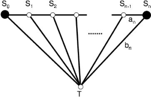
Figure 1: The Brecht-Colbourn ladder.

Refer to caption
Figure 2: The generalized fan.

In this work, we give the exact two-terminal reliability of two well-known graphs, namely the Brecht-Colbourn ladder [13, 14, 52] and the generalized fan [3, 49], which have the same all-terminal reliability. Both networks have been studied in the literature, especially the first one, as a case study for different lower bounds of the two-terminal reliability [14], but with a limited number of nodes. Here, the number of nodes will be arbitrary. Our solution fully exploits the recursive nature of the graphs and the triangle-star transformation with unreliable nodes [34]. The final expressions are products of (at most) 4×4444\times 4 transfer matrices, in which the arbitrary reliability of each node and edge appears explicitly. In the case of identical edge (p𝑝p) and node (ρ𝜌\rho) reliabilities, we provide the generating functions of the two-terminal reliabilities, leading to a very simple expression for the generalized fan. Another byproduct is the asymptotic locations of the zeros of the two-terminal reliability polynomials for the Brecht-Colbourn ladder and the generalized fan, which exhibit very different structures and undergo a structural transition at ρ=12𝜌12\displaystyle\rho=\frac{1}{2}.

Our aim is (i) to give a detailed derivation of the final results, so that people involved in reliability studies can readily use an easy-to-implement formula (ii) compare the exact solution with previous results (iii) exhibit the structural changes undergone by the location of the zeros of reliability polynomials as a function of node reliability (iv) emphasize anew the importance of algebraic structures of the underlying graphs in the determination of their associated polynomials [10, 59].

Our paper is organized as follows : In Section 2, we briefly recall the formulae for the triangle-star transformation for unreliable nodes. In Section 3, we define the notations for the different edge and node reliabilities and detail the derivation of the main results (eqs. (12) and (14) for the Brecht-Colbourn ladder, eqs. (23) and (25) for the generalized fan). Section 4 is devoted to the case where all edges and nodes have identical reliabilities p𝑝p and ρ𝜌\rho, respectively, the size of the network appearing simply as an integer n𝑛n. We give the analytical solution of the two-terminal reliability Rel2(p,ρ;n)subscriptRel2𝑝𝜌𝑛{\rm Rel}_{2}(p,\rho;n) for the Brecht-Colbourn ladder and the generalized fan, and the associated generating functions, which encode all the necessary information in a beautifully simple, compact form. The asymptotic power-law or constant behaviors are given when n𝑛n\rightarrow\infty. Prompted by the nearly universal character of the Brown-Colbourn conjecture [16], we address in Section 5 the location of zeros of the two-terminal reliability polynomials, and show that their structures are very different even though their internal structure is similar. For the sake of completeness, we derive in Section 6 the common all-terminal reliability for both networks, for arbitrary values of edge reliabilities. Finally, we conclude by indicating several directions in which the present results may be further extended, so that, for instance, a catalog of exactly solvable networks — in terms of reliability — may be given rapidly [69]. Such a catalog of elementary bricks could be useful for a new and improved set of bounds or benchmarks for alternative methods in the general case.

2 Triangle-star transformation for unreliable nodes

The triangle-star — also called delta-wye or ΔYΔY\Delta-{\rm Y} — transformation has been used many times to simplify calculations of network reliability [20, 26, 31, 34, 42, 55, 72]. It has mostly been applied in a perfect nodes context, to provide upper and lower bounds to the exact reliability. Here, we exploit this transformation to the full in the case of imperfect nodes in order to obtain exact results. Since it plays a crucial part of the derivation, we give the formulae derived by Gadani [34].

Refer to caption
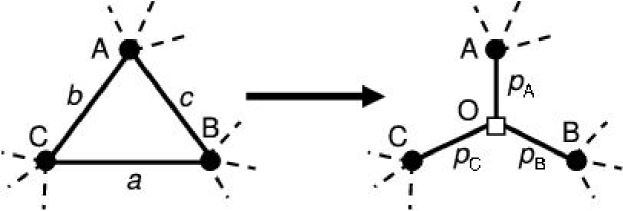
Figure 3: Triangle-star transformation for unreliable nodes. A𝐴A, B𝐵B, and C𝐶C are the node reliabilities, with a𝑎a, b𝑏b, and c𝑐c the edge reliabilities of the initial network, and pAsubscript𝑝𝐴p_{A}, pBsubscript𝑝𝐵p_{B}, pCsubscript𝑝𝐶p_{C}, and O𝑂O, those of the transformed network.

Let us consider three particular nodes A𝐴A, B𝐵B, and C𝐶C of a network, connected as shown in the left part of Fig. 3 (the reliability of the nodes are given by the same uppercase variables, so as to prevent an unnecessary multiplication of notations). The reliability of the edge connecting A𝐴A and B𝐵B is given by (lowercase) c𝑐c, with similar notation for the remaining edges of the triangle. The aim of the triangle-star transformation is to replace the triangle by a star, which is possible by the addition of a new unreliable node O𝑂O and three new edges connecting O𝑂O to A𝐴A, B𝐵B, and C𝐶C, with reliabilities pAsubscript𝑝𝐴p_{A}, pBsubscript𝑝𝐵p_{B}, and pCsubscript𝑝𝐶p_{C}, respectively. Both networks are equivalent provided that the following compatibility relations hold [34]

pAOpCsubscript𝑝𝐴𝑂subscript𝑝𝐶\displaystyle p_{A}\,O\,p_{C} =\displaystyle= b+acBabcB,𝑏𝑎𝑐𝐵𝑎𝑏𝑐𝐵\displaystyle b+a\,c\,B-a\,b\,c\,B, (1)
pAOpBsubscript𝑝𝐴𝑂subscript𝑝𝐵\displaystyle p_{A}\,O\,p_{B} =\displaystyle= c+abCabcC,𝑐𝑎𝑏𝐶𝑎𝑏𝑐𝐶\displaystyle c+a\,b\,C-a\,b\,c\,C, (2)
pBOpCsubscript𝑝𝐵𝑂subscript𝑝𝐶\displaystyle p_{B}\,O\,p_{C} =\displaystyle= a+bcAabcA,𝑎𝑏𝑐𝐴𝑎𝑏𝑐𝐴\displaystyle a+b\,c\,A-a\,b\,c\,A, (3)
pAOpBpCsubscript𝑝𝐴𝑂subscript𝑝𝐵subscript𝑝𝐶\displaystyle p_{A}\,O\,p_{B}\,p_{C} =\displaystyle= ab+bc+ac2abc.𝑎𝑏𝑏𝑐𝑎𝑐2𝑎𝑏𝑐\displaystyle a\,b+b\,c+a\,c-2\,a\,b\,c. (4)

Note that the first three equalities correspond to the probability that the two nodes under consideration are connected, while the last one gives the probability that the three nodes are connected. A word of caution — already given by Gadani — is worth mentioning in the case of successive triangle-star transformation: the triangles should have no common edge or node.

3 Derivation of the main results

3.1 Brecht-Colbourn ladder

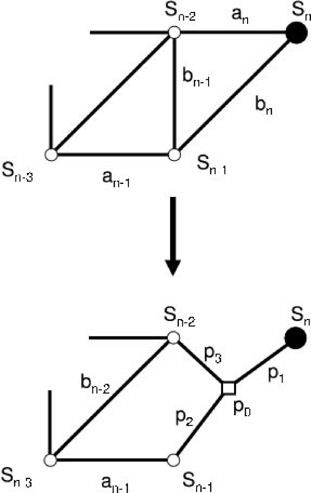
Let us first name the different edge and node reliabilities of the Brecht-Colbourn ladder, and detail how we can use the triangle-star transformation of the preceding section. Assuming that S0subscript𝑆0S_{0} is always the source node, and using node reliabilities Sisubscript𝑆𝑖S_{i}, we note ansubscript𝑎𝑛a_{n} the reliability of the edge (Sn2,Sn)subscript𝑆𝑛2subscript𝑆𝑛(S_{n-2},S_{n}), and bnsubscript𝑏𝑛b_{n} that of (Sn1,Sn)subscript𝑆𝑛1subscript𝑆𝑛(S_{n-1},S_{n}), as shown at the top of Fig. 4.


Refer to caption
Figure 4: Decomposition of the ladder using the triangle-star transformation.

The application of the triangle-star transformation to Fig. 4 leads to

p1p0p2subscript𝑝1subscript𝑝0subscript𝑝2\displaystyle p_{1}\,p_{0}\,p_{2} =\displaystyle= bn+anbn1Sn2anbn1bnSn2,subscript𝑏𝑛subscript𝑎𝑛subscript𝑏𝑛1subscript𝑆𝑛2subscript𝑎𝑛subscript𝑏𝑛1subscript𝑏𝑛subscript𝑆𝑛2\displaystyle b_{n}+a_{n}\,b_{n-1}\,S_{n-2}-a_{n}\,b_{n-1}\,b_{n}\,S_{n-2}, (5)
p1p0p3subscript𝑝1subscript𝑝0subscript𝑝3\displaystyle p_{1}\,p_{0}\,p_{3} =\displaystyle= an+bn1bnSn1anbn1bnSn1,subscript𝑎𝑛subscript𝑏𝑛1subscript𝑏𝑛subscript𝑆𝑛1subscript𝑎𝑛subscript𝑏𝑛1subscript𝑏𝑛subscript𝑆𝑛1\displaystyle a_{n}+b_{n-1}\,b_{n}\,S_{n-1}-a_{n}\,b_{n-1}\,b_{n}\,S_{n-1}, (6)
p1p0p2p3subscript𝑝1subscript𝑝0subscript𝑝2subscript𝑝3\displaystyle p_{1}\,p_{0}\,p_{2}\,p_{3} =\displaystyle= anbn+anbn1+bn1bn2anbn1bn.subscript𝑎𝑛subscript𝑏𝑛subscript𝑎𝑛subscript𝑏𝑛1subscript𝑏𝑛1subscript𝑏𝑛2subscript𝑎𝑛subscript𝑏𝑛1subscript𝑏𝑛\displaystyle a_{n}\,b_{n}+a_{n}\,b_{n-1}+b_{n-1}\,b_{n}-2\,a_{n}\,b_{n-1}\,b_{n}. (7)

Writing the two-terminal reliability Rel2(BC)(S0Sn)=Sn𝒮nsuperscriptsubscriptRel2BCsubscript𝑆0subscript𝑆𝑛subscript𝑆𝑛subscript𝒮𝑛{\rm Rel}_{2}^{{\rm(BC)}}(S_{0}\rightarrow S_{n})=S_{n}\,{\mathcal{S}}_{n}, we immediately see that

𝒮n=p1p0𝒮n1(an1an1Sn1p2,bn1p3),subscript𝒮𝑛subscript𝑝1subscript𝑝0subscript𝒮𝑛1formulae-sequencesubscript𝑎𝑛1subscript𝑎𝑛1subscript𝑆𝑛1subscript𝑝2subscript𝑏𝑛1subscript𝑝3{\mathcal{S}}_{n}=p_{1}\,p_{0}\,{\mathcal{S}}_{n-1}(a_{n-1}\rightarrow a_{n-1}\,S_{n-1}\,p_{2},b_{n-1}\rightarrow p_{3}), (8)

because the transformed graph remains essentially a Brecht-Colbourn ladder, provided that some edges are renormalized (bn1subscript𝑏𝑛1b_{n-1} must be replaced by p3subscript𝑝3p_{3}, Sn1subscript𝑆𝑛1S_{n-1} by p0subscript𝑝0p_{0}, and an1subscript𝑎𝑛1a_{n-1} by an1Sn1p2subscript𝑎𝑛1subscript𝑆𝑛1subscript𝑝2a_{n-1}\,S_{n-1}\,p_{2}).

In the case of imperfect nodes, the assumption

𝒮n=αnan+α~nanSn1+β~nbnSn1+γ~nanbnSn1subscript𝒮𝑛subscript𝛼𝑛subscript𝑎𝑛subscript~𝛼𝑛subscript𝑎𝑛subscript𝑆𝑛1subscript~𝛽𝑛subscript𝑏𝑛subscript𝑆𝑛1subscript~𝛾𝑛subscript𝑎𝑛subscript𝑏𝑛subscript𝑆𝑛1{\mathcal{S}}_{n}=\alpha_{n}\,a_{n}+\widetilde{\alpha}_{n}\,a_{n}\,S_{n-1}+\widetilde{\beta}_{n}\,b_{n}\,S_{n-1}+\widetilde{\gamma}_{n}\,a_{n}\,b_{n}\,S_{n-1} (9)

gives four parameters, for which we want to find a recursion relation. When we use eqs. (5)–(7) in eq. (9), there is one slightly tricky point: we are actually dealing with Boolean functions, so that Sn22Sn2superscriptsubscript𝑆𝑛22subscript𝑆𝑛2S_{n-2}^{2}\equiv S_{n-2} (see for instance [3]) and

p1p0α~n1Sn2(an1Sn1p2)subscript𝑝1subscript𝑝0subscript~𝛼𝑛1subscript𝑆𝑛2subscript𝑎𝑛1subscript𝑆𝑛1subscript𝑝2\displaystyle\hskip-56.9055ptp_{1}\,p_{0}\,\widetilde{\alpha}_{n-1}\,S_{n-2}\,\left(a_{n-1}\,S_{n-1}\,p_{2}\right) (10)
=\displaystyle= α~n1Sn1Sn2an1(bn+anbn1Sn2anbn1bnSn2)subscript~𝛼𝑛1subscript𝑆𝑛1subscript𝑆𝑛2subscript𝑎𝑛1subscript𝑏𝑛subscript𝑎𝑛subscript𝑏𝑛1subscript𝑆𝑛2subscript𝑎𝑛subscript𝑏𝑛1subscript𝑏𝑛subscript𝑆𝑛2\displaystyle\widetilde{\alpha}_{n-1}\,S_{n-1}\,S_{n-2}\,a_{n-1}\,(b_{n}+a_{n}\,b_{n-1}\,S_{n-2}-a_{n}\,b_{n-1}\,b_{n}\,S_{n-2})
\displaystyle\equiv α~n1Sn1Sn2an1(bn+anbn1anbn1bn).subscript~𝛼𝑛1subscript𝑆𝑛1subscript𝑆𝑛2subscript𝑎𝑛1subscript𝑏𝑛subscript𝑎𝑛subscript𝑏𝑛1subscript𝑎𝑛subscript𝑏𝑛1subscript𝑏𝑛\displaystyle\widetilde{\alpha}_{n-1}\,S_{n-1}\,S_{n-2}\,a_{n-1}\,(b_{n}+a_{n}\,b_{n-1}-a_{n}\,b_{n-1}\,b_{n}).

We deduce

(αnα~nβ~nγ~n)=Mn1(αn1α~n1β~n1γ~n1),subscript𝛼𝑛subscript~𝛼𝑛subscript~𝛽𝑛subscript~𝛾𝑛subscript𝑀𝑛1subscript𝛼𝑛1subscript~𝛼𝑛1subscript~𝛽𝑛1subscript~𝛾𝑛1\left(\begin{array}[]{c}\alpha_{n}\\ \widetilde{\alpha}_{n}\\ \widetilde{\beta}_{n}\\ \widetilde{\gamma}_{n}\end{array}\right)\;=\;M_{n-1}\;\cdot\;\left(\begin{array}[]{c}\alpha_{n-1}\\ \widetilde{\alpha}_{n-1}\\ \widetilde{\beta}_{n-1}\\ \widetilde{\gamma}_{n-1}\end{array}\right), (11)

where the 4×4444\times 4 transfer matrix Mn1subscript𝑀𝑛1M_{n-1} is given by

Mn1=(00Sn20an1bn1Sn2an1bn1Sn20an1bn1Sn2an1an1Sn2bn1Sn2an1bn1Sn2an1bn1Sn2an1bn1Sn2bn1Sn2an1(12bn1)Sn2).subscript𝑀𝑛100subscript𝑆𝑛20missing-subexpressionmissing-subexpressionmissing-subexpressionmissing-subexpressionsubscript𝑎𝑛1subscript𝑏𝑛1subscript𝑆𝑛2subscript𝑎𝑛1subscript𝑏𝑛1subscript𝑆𝑛20subscript𝑎𝑛1subscript𝑏𝑛1subscript𝑆𝑛2missing-subexpressionmissing-subexpressionmissing-subexpressionmissing-subexpressionsubscript𝑎𝑛1subscript𝑎𝑛1subscript𝑆𝑛2subscript𝑏𝑛1subscript𝑆𝑛2subscript𝑎𝑛1subscript𝑏𝑛1subscript𝑆𝑛2missing-subexpressionmissing-subexpressionmissing-subexpressionmissing-subexpressionsubscript𝑎𝑛1subscript𝑏𝑛1subscript𝑆𝑛2subscript𝑎𝑛1subscript𝑏𝑛1subscript𝑆𝑛2subscript𝑏𝑛1subscript𝑆𝑛2subscript𝑎𝑛112subscript𝑏𝑛1subscript𝑆𝑛2M_{n-1}=\left(\begin{array}[]{l|l|l|l}0&0&S_{n-2}&0\\ \hline\cr a_{n-1}\,b_{n-1}\,S_{n-2}&a_{n-1}\,b_{n-1}\,S_{n-2}&0&a_{n-1}\,b_{n-1}\,S_{n-2}\\ \hline\cr a_{n-1}&a_{n-1}\,S_{n-2}&b_{n-1}\,S_{n-2}&a_{n-1}\,b_{n-1}\,S_{n-2}\\ \hline\cr-a_{n-1}\,b_{n-1}\,S_{n-2}&-a_{n-1}\,b_{n-1}\,S_{n-2}&-b_{n-1}\,S_{n-2}&a_{n-1}\,(1-2\,b_{n-1})\,S_{n-2}\end{array}\right). (12)

For n=2𝑛2n=2, the two-terminal reliability is easily solved because we have series-parallel graph:

Rel2(BC)(S0S2)=S2(a2+b1S1b2a2b1S1b2)S0,superscriptsubscriptRel2BCsubscript𝑆0subscript𝑆2subscript𝑆2subscript𝑎2subscript𝑏1subscript𝑆1subscript𝑏2subscript𝑎2subscript𝑏1subscript𝑆1subscript𝑏2subscript𝑆0{\rm Rel}_{2}^{{\rm(BC)}}(S_{0}\rightarrow S_{2})=S_{2}\,(a_{2}+b_{1}\,S_{1}\,b_{2}-a_{2}\,b_{1}\,S_{1}\,b_{2})\,S_{0}, (13)

which leads to α2=S0subscript𝛼2subscript𝑆0\alpha_{2}=S_{0}, α~2=0subscript~𝛼20\widetilde{\alpha}_{2}=0, β~2=b1S0subscript~𝛽2subscript𝑏1subscript𝑆0\widetilde{\beta}_{2}=b_{1}\,S_{0}, and γ~2=b1S0subscript~𝛾2subscript𝑏1subscript𝑆0\widetilde{\gamma}_{2}=-b_{1}\,S_{0}, or equivalently to α1=α~1=γ~1=0subscript𝛼1subscript~𝛼1subscript~𝛾10\alpha_{1}=\widetilde{\alpha}_{1}=\widetilde{\gamma}_{1}=0 et β~1=1subscript~𝛽11\widetilde{\beta}_{1}=1 (see eq. (12)). The final result is

Rel2(BC)(S0Sn)=Sn(0 0 1 0)MnMn1M1(0010).superscriptsubscriptRel2BCsubscript𝑆0subscript𝑆𝑛subscript𝑆𝑛0010subscript𝑀𝑛subscript𝑀𝑛1subscript𝑀10010{\rm Rel}_{2}^{{\rm(BC)}}(S_{0}\rightarrow S_{n})=S_{n}\,(0\;0\;1\;0)\cdot M_{n}\,\cdot\,M_{n-1}\;\;\cdots\;\;M_{1}\,\cdot\left(\begin{array}[]{c}0\\ 0\\ 1\\ 0\end{array}\right). (14)

Note that in M1subscript𝑀1M_{1}, a1subscript𝑎1a_{1} is quite arbitrary, so that it can be set equal to zero without loss of generality. Equation (14) also holds for n𝑛n equal to 1 or even 0 (following a frequent convention that a product of zero matrices is the identity matrix); it has also been independently checked for the first values of n𝑛n, using a sum of disjoint products procedure.

In the case of perfect nodes, the ansatz should be 𝒮n=αnan+βnbn+γnanbnsubscript𝒮𝑛subscript𝛼𝑛subscript𝑎𝑛subscript𝛽𝑛subscript𝑏𝑛subscript𝛾𝑛subscript𝑎𝑛subscript𝑏𝑛{\mathcal{S}}_{n}=\alpha_{n}\,a_{n}+\beta_{n}\,b_{n}+\gamma_{n}\,a_{n}\,b_{n}. The relevant 3×3333\times 3 transfer matrix Mnsubscriptsuperscript𝑀𝑛{M^{\prime}}_{n} is now

Mn=(anbn1anbnanbnanbnanbnbnan(12bn)),subscriptsuperscript𝑀𝑛subscript𝑎𝑛subscript𝑏𝑛1subscript𝑎𝑛subscript𝑏𝑛missing-subexpressionmissing-subexpressionmissing-subexpressionsubscript𝑎𝑛subscript𝑏𝑛subscript𝑎𝑛subscript𝑏𝑛missing-subexpressionmissing-subexpressionmissing-subexpressionsubscript𝑎𝑛subscript𝑏𝑛subscript𝑏𝑛subscript𝑎𝑛12subscript𝑏𝑛{M^{\prime}}_{n}=\left(\begin{array}[]{c|c|c}a_{n}\,b_{n}&1&a_{n}\,b_{n}\\ \hline\cr a_{n}&b_{n}&a_{n}\,b_{n}\\ \hline\cr-a_{n}\,b_{n}&-b_{n}&a_{n}\,(1-2\,b_{n})\end{array}\right), (15)

from which we deduce

Rel2(BC)(S0Sn;perfectnodes)=(0 1 0)MnMn1M1(010).superscriptsubscriptRel2BCsubscript𝑆0subscript𝑆𝑛perfectnodes010subscriptsuperscript𝑀𝑛subscriptsuperscript𝑀𝑛1subscriptsuperscript𝑀1010{\rm Rel}_{2}^{{\rm(BC)}}(S_{0}\rightarrow S_{n};{\rm perfect\ nodes})=(0\;1\;0)\cdot{M^{\prime}}_{n}\,\cdot\,{M^{\prime}}_{n-1}\;\;\cdots\;\;{M^{\prime}}_{1}\,\cdot\left(\begin{array}[]{c}0\\ 1\\ 0\end{array}\right). (16)

3.2 Generalized fan


Refer to caption
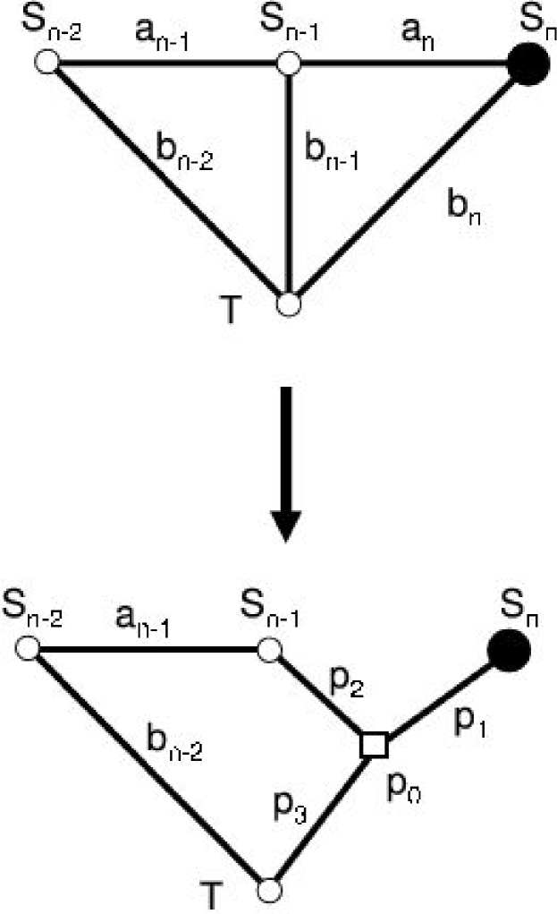
Figure 5: Triangle-star transformation for the generalized fan.

Let us now turn to the second architecture. The triangle-star transformation, applied to the generalized fan, is displayed on Fig. 5, and we expect the common node T𝑇T to play a special role in the recursion relation. We can write Rel2(fan)(S0Sn)=Sn𝒮^nsuperscriptsubscriptRel2fansubscript𝑆0subscript𝑆𝑛subscript𝑆𝑛subscript^𝒮𝑛{\rm Rel}_{2}^{{\rm(fan)}}(S_{0}\rightarrow S_{n})=S_{n}\;\widehat{{\mathcal{S}}}_{n}, and see immediately that

𝒮^n=p1p0𝒮^n1(an1an1Sn1p2,bn1p3),subscript^𝒮𝑛subscript𝑝1subscript𝑝0subscript^𝒮𝑛1formulae-sequencesubscript𝑎𝑛1subscript𝑎𝑛1subscript𝑆𝑛1subscript𝑝2subscript𝑏𝑛1subscript𝑝3\widehat{{\mathcal{S}}}_{n}=p_{1}\,p_{0}\,\widehat{{\mathcal{S}}}_{n-1}(a_{n-1}\rightarrow a_{n-1}\,S_{n-1}\,p_{2},b_{n-1}\rightarrow p_{3}), (17)

with

p1p0p2subscript𝑝1subscript𝑝0subscript𝑝2\displaystyle p_{1}\,p_{0}\,p_{2} =\displaystyle= an+bn1bnTanbn1bnT,subscript𝑎𝑛subscript𝑏𝑛1subscript𝑏𝑛𝑇subscript𝑎𝑛subscript𝑏𝑛1subscript𝑏𝑛𝑇\displaystyle a_{n}+b_{n-1}\,b_{n}\,T-a_{n}\,b_{n-1}\,b_{n}\,T, (18)
p1p0p3subscript𝑝1subscript𝑝0subscript𝑝3\displaystyle p_{1}\,p_{0}\,p_{3} =\displaystyle= bn+anbn1Sn1anbn1bnSn1,subscript𝑏𝑛subscript𝑎𝑛subscript𝑏𝑛1subscript𝑆𝑛1subscript𝑎𝑛subscript𝑏𝑛1subscript𝑏𝑛subscript𝑆𝑛1\displaystyle b_{n}+a_{n}\,b_{n-1}\,S_{n-1}-a_{n}\,b_{n-1}\,b_{n}\,S_{n-1}, (19)
p1p0p2p3subscript𝑝1subscript𝑝0subscript𝑝2subscript𝑝3\displaystyle p_{1}\,p_{0}\,p_{2}\,p_{3} =\displaystyle= anbn+anbn1+bn1bn2anbn1bn.subscript𝑎𝑛subscript𝑏𝑛subscript𝑎𝑛subscript𝑏𝑛1subscript𝑏𝑛1subscript𝑏𝑛2subscript𝑎𝑛subscript𝑏𝑛1subscript𝑏𝑛\displaystyle a_{n}\,b_{n}+a_{n}\,b_{n-1}+b_{n-1}\,b_{n}-2\,a_{n}\,b_{n-1}\,b_{n}. (20)

Our ansatz is now

𝒮^n=Snαnan+α~nanT+β~nbnT+γ~nanbnT.subscript^𝒮𝑛subscript𝑆𝑛subscript𝛼𝑛subscript𝑎𝑛subscript~𝛼𝑛subscript𝑎𝑛𝑇subscript~𝛽𝑛subscript𝑏𝑛𝑇subscript~𝛾𝑛subscript𝑎𝑛subscript𝑏𝑛𝑇\widehat{{\mathcal{S}}}_{n}=S_{n}\,\alpha_{n}\,a_{n}+\widetilde{\alpha}_{n}\,a_{n}\,T+\widetilde{\beta}_{n}\,b_{n}\,T+\widetilde{\gamma}_{n}\,a_{n}\,b_{n}\,T. (21)

Here again, we must be careful with the Boolean variable T𝑇T. When using eq. (18) in eq. (21), all occurrences of T2superscript𝑇2T^{2} must be replaced by T𝑇T. The recursion relations take the now familiar form

(αnα~nβ~nγ~n)=M^n1(αn1α~n1β~n1γ~n1),subscript𝛼𝑛subscript~𝛼𝑛subscript~𝛽𝑛subscript~𝛾𝑛subscript^𝑀𝑛1subscript𝛼𝑛1subscript~𝛼𝑛1subscript~𝛽𝑛1subscript~𝛾𝑛1\left(\begin{array}[]{c}\alpha_{n}\\ \widetilde{\alpha}_{n}\\ \widetilde{\beta}_{n}\\ \widetilde{\gamma}_{n}\end{array}\right)=\widehat{M}_{n-1}\cdot\left(\begin{array}[]{c}\alpha_{n-1}\\ \widetilde{\alpha}_{n-1}\\ \widetilde{\beta}_{n-1}\\ \widetilde{\gamma}_{n-1}\end{array}\right), (22)

where the transfer matrix M^nsubscript^𝑀𝑛\widehat{M}_{n} is

M^n=(anSn0000anSnbnSnanbnSnanbnSnanbnSn1anbnSnanbnSnanbnSnbnSnan(12bn)Sn).subscript^𝑀𝑛subscript𝑎𝑛subscript𝑆𝑛000missing-subexpressionmissing-subexpressionmissing-subexpressionmissing-subexpression0subscript𝑎𝑛subscript𝑆𝑛subscript𝑏𝑛subscript𝑆𝑛subscript𝑎𝑛subscript𝑏𝑛subscript𝑆𝑛missing-subexpressionmissing-subexpressionmissing-subexpressionmissing-subexpressionsubscript𝑎𝑛subscript𝑏𝑛subscript𝑆𝑛subscript𝑎𝑛subscript𝑏𝑛subscript𝑆𝑛1subscript𝑎𝑛subscript𝑏𝑛subscript𝑆𝑛missing-subexpressionmissing-subexpressionmissing-subexpressionmissing-subexpressionsubscript𝑎𝑛subscript𝑏𝑛subscript𝑆𝑛subscript𝑎𝑛subscript𝑏𝑛subscript𝑆𝑛subscript𝑏𝑛subscript𝑆𝑛subscript𝑎𝑛12subscript𝑏𝑛subscript𝑆𝑛\widehat{M}_{n}=\left(\begin{array}[]{c|c|c|c}a_{n}\,S_{n}&0&0&0\\ \hline\cr 0&a_{n}\,S_{n}&b_{n}\,S_{n}&a_{n}\,b_{n}\,S_{n}\\ \hline\cr a_{n}\,b_{n}\,S_{n}&a_{n}\,b_{n}\,S_{n}&1&a_{n}\,b_{n}\,S_{n}\\ \hline\cr-a_{n}\,b_{n}\,S_{n}&-a_{n}\,b_{n}\,S_{n}&-b_{n}\,S_{n}&a_{n}\,(1-2\,b_{n})\,S_{n}\end{array}\right). (23)

When n=1𝑛1n=1, we have a series-parallel graph:

Rel2(fan)(S0S1)=S1(a1+b0b1Ta1b0b1T)S0,superscriptsubscriptRel2fansubscript𝑆0subscript𝑆1subscript𝑆1subscript𝑎1subscript𝑏0subscript𝑏1𝑇subscript𝑎1subscript𝑏0subscript𝑏1𝑇subscript𝑆0{\rm Rel}_{2}^{{\rm(fan)}}(S_{0}\rightarrow S_{1})=S_{1}(a_{1}+b_{0}\,b_{1}\,T-a_{1}\,b_{0}\,b_{1}\,T)\,S_{0}, (24)

from which we deduce the final expression

Rel2(fan)(S0Sn)=(1T 0 0)M^nM^n1M^1M^0(1000),superscriptsubscriptRel2fansubscript𝑆0subscript𝑆𝑛1𝑇00subscript^𝑀𝑛subscript^𝑀𝑛1subscript^𝑀1subscript^𝑀01000{\rm Rel}_{2}^{{\rm(fan)}}(S_{0}\rightarrow S_{n})=(1\;T\;0\;0)\,\cdot\,\widehat{M}_{n}\,\cdot\widehat{M}_{n-1}\;\cdots\;\widehat{M}_{1}\,\cdot\,\widehat{M}_{0}\,\cdot\,\left(\begin{array}[]{c}1\\ 0\\ 0\\ 0\end{array}\right), (25)

with the additional convention a01subscript𝑎01a_{0}\equiv 1 for M^0subscript^𝑀0\widehat{M}_{0}. We have also checked the correctness of eq. (25) by a sum of disjoint products procedure for the first values of n𝑛n. It also agrees with the expression of Aggarwal et al. [3] for n=3𝑛3n=3.

In the case of perfect nodes, which is often considered in the literature, the ansatz 𝒮^n=αnan+βnbn+γnanbnsubscript^𝒮𝑛subscript𝛼𝑛subscript𝑎𝑛subscript𝛽𝑛subscript𝑏𝑛subscript𝛾𝑛subscript𝑎𝑛subscript𝑏𝑛\widehat{{\mathcal{S}}}_{n}=\alpha_{n}\,a_{n}+\beta_{n}\,b_{n}+\gamma_{n}\,a_{n}\,b_{n} leads to

Rel2(fan)(S0Sn;perfectnodes)=(1 0 0)M^nM^n1M^1M^0(100),superscriptsubscriptRel2fansubscript𝑆0subscript𝑆𝑛perfectnodes100subscript^superscript𝑀𝑛subscript^superscript𝑀𝑛1subscript^superscript𝑀1subscript^superscript𝑀0100{\rm Rel}_{2}^{{\rm(fan)}}(S_{0}\rightarrow S_{n};{\rm perfect\ nodes})=(1\;0\;0)\,\cdot\,\widehat{M^{\prime}}_{n}\,\cdot\widehat{M^{\prime}}_{n-1}\;\cdots\;\widehat{M^{\prime}}_{1}\,\cdot\,\widehat{M^{\prime}}_{0}\,\cdot\,\left(\begin{array}[]{c}1\\ 0\\ 0\end{array}\right), (26)

with

M^n=(anbnanbnanbn1anbnanbnbnan(12bn)),subscript^superscript𝑀𝑛subscript𝑎𝑛subscript𝑏𝑛subscript𝑎𝑛subscript𝑏𝑛missing-subexpressionmissing-subexpressionmissing-subexpressionsubscript𝑎𝑛subscript𝑏𝑛1subscript𝑎𝑛subscript𝑏𝑛missing-subexpressionmissing-subexpressionmissing-subexpressionsubscript𝑎𝑛subscript𝑏𝑛subscript𝑏𝑛subscript𝑎𝑛12subscript𝑏𝑛\widehat{M^{\prime}}_{n}=\left(\begin{array}[]{c|c|c}a_{n}&b_{n}&a_{n}\,b_{n}\\ \hline\cr a_{n}\,b_{n}&1&a_{n}\,b_{n}\\ \hline\cr-a_{n}\,b_{n}&-b_{n}&a_{n}\,(1-2\,b_{n})\end{array}\right), (27)

and again a01subscript𝑎01a_{0}\equiv 1 for M^0subscript^𝑀0\widehat{M}_{0}.

It is worth noting that while the sizes of Mnsubscript𝑀𝑛M_{n} and M^nsubscript^𝑀𝑛\widehat{M}_{n} for the Brecht-Colbourn and fan cases are identical, their matrix elements are clearly distinct. This actually leads to strong differences, as will be shown in the following section.

4 Identical reliabilities p𝑝p and ρ𝜌\rho

4.1 Introduction

While eqs. (12) and (14) give the two-terminal reliability for the general Brecht-Colbourn ladder, and eqs. (23) and (25) for the fan, we consider here the special case where all edges and nodes have reliabilities p𝑝p and ρ𝜌\rho, respectively. Because identical edge reliabilities are usually taken for granted, our exact results may help to demonstrate once again the underlying connection between combinatorics and reliability theory, most particularly in the enumeration of self-avoiding walks [26, 35, 52]. This assumption greatly simplifies the problem, since all transfer matrices, with the exception of M^0subscript^𝑀0\widehat{M}_{0} in the case of the generalized fan, are identical to a matrix M(p,ρ)𝑀𝑝𝜌M(p,\rho) (or M^(p,ρ)^𝑀𝑝𝜌\widehat{M}(p,\rho)): the two-terminal reliability is essentially the nthsuperscript𝑛thn^{\rm th} power of one matrix. While the determination of its eigenvalues and eigenvectors is one way to solve the problem, we adopt in the following the generating function formalism, which is a fundamental tool in combinatorics [65], and makes for a very compact synthesis of the results. The generating function G(z)𝐺𝑧G(z) is defined by

G(z)=n=0Rel2(n)(p,ρ)zn.𝐺𝑧superscriptsubscript𝑛0superscriptsubscriptRel2𝑛𝑝𝜌superscript𝑧𝑛G(z)=\sum_{n=0}^{\infty}{\rm Rel}_{2}^{(n)}(p,\rho)\,z^{n}. (28)

From the finite-order recursion relations obeyed by Rel2(n)superscriptsubscriptRel2𝑛{\rm Rel}_{2}^{(n)}, the generating function is obviously a rational function of z𝑧z, namely G(z)=N(z)/D(z)𝐺𝑧𝑁𝑧𝐷𝑧G(z)=N(z)/D(z). In the present study, its denominator is at most of degree 4 in z𝑧z, because in the absence of further simplification, D(z)=z4Pcarac(1/z)𝐷𝑧superscript𝑧4subscript𝑃carac1𝑧D(z)=z^{4}\,P_{\rm carac}(1/z), where Pcaracsubscript𝑃caracP_{\rm carac} is the characteristic polynomial of the transfer matrix. The determination of N(z)𝑁𝑧N(z) is then very straightforward: we only need to multiply the first terms of the expansion of G(z)𝐺𝑧G(z) by D(z)𝐷𝑧D(z) to see the numerator N(z)𝑁𝑧N(z) emerge. The partial fraction decomposition of G(z)𝐺𝑧G(z) finally leads to a compact, sometimes very simple, analytical expression of Rel2(n)(p,ρ)superscriptsubscriptRel2𝑛𝑝𝜌{\rm Rel}_{2}^{(n)}(p,\rho), for arbitrary n𝑛n.

4.2 Brecht-Colbourn ladder

4.2.1 Imperfect nodes and edges

When edge and node reliabilities are p𝑝p et ρ𝜌\rho, the transfer matrix of eq. (12) is equal to

M(p,ρ)=(00ρ0p2ρp2ρ0p2ρppρpρp2ρp2ρp2ρpρp(12p)ρ),𝑀𝑝𝜌00𝜌0missing-subexpressionmissing-subexpressionmissing-subexpressionmissing-subexpressionsuperscript𝑝2𝜌superscript𝑝2𝜌0superscript𝑝2𝜌missing-subexpressionmissing-subexpressionmissing-subexpressionmissing-subexpression𝑝𝑝𝜌𝑝𝜌superscript𝑝2𝜌missing-subexpressionmissing-subexpressionmissing-subexpressionmissing-subexpressionsuperscript𝑝2𝜌superscript𝑝2𝜌𝑝𝜌𝑝12𝑝𝜌M(p,\rho)=\left(\begin{array}[]{l|l|l|l}0&0&\rho&0\\ \hline\cr p^{2}\,\rho&p^{2}\,\rho&0&p^{2}\,\rho\\ \hline\cr p&p\,\rho&p\,\rho&p^{2}\,\rho\\ \hline\cr-p^{2}\,\rho&-p^{2}\,\rho&-p\,\rho&p\,(1-2\,p)\,\rho\end{array}\right), (29)

and

Rel2(S0Sn)=ρ(0 0 1 0)M(p,ρ)n(0010).subscriptRel2subscript𝑆0subscript𝑆𝑛𝜌0010𝑀superscript𝑝𝜌𝑛0010{\rm Rel}_{2}(S_{0}\rightarrow S_{n})=\rho\,(0\;0\;1\;0)\cdot M(p,\rho)^{n}\,\cdot\left(\begin{array}[]{c}0\\ 0\\ 1\\ 0\end{array}\right). (30)

The characteristic polynomial of this matrix is

Pcarac(BC)(p,ρ;x)superscriptsubscript𝑃caracBC𝑝𝜌𝑥\displaystyle P_{\rm carac}^{\rm(BC)}(p,\rho;x) =\displaystyle= x4p(2p)ρx3pρ(1ρ(p+p2p3))x2superscript𝑥4𝑝2𝑝𝜌superscript𝑥3𝑝𝜌1𝜌𝑝superscript𝑝2superscript𝑝3superscript𝑥2\displaystyle x^{4}-p\,(2-p)\,\rho\,x^{3}-p\,\rho\,\big{(}1-\rho\,(p+p^{2}-p^{3})\big{)}\,x^{2} (31)
+(1p)(1pρ)p2ρ2x(1p)(1ρ)p4ρ3.1𝑝1𝑝𝜌superscript𝑝2superscript𝜌2𝑥1𝑝1𝜌superscript𝑝4superscript𝜌3\displaystyle+(1-p)\,(1-p\,\rho)\,p^{2}\,\rho^{2}\,x-(1-p)\,(1-\rho)\,p^{4}\,\rho^{3}.

The eigenvalues of M(p,ρ)𝑀𝑝𝜌M(p,\rho) are given by the roots of this polynomial of degree 4. From the first few values of Rel2(S0Sn)subscriptRel2subscript𝑆0subscript𝑆𝑛{\rm Rel}_{2}(S_{0}\rightarrow S_{n}) (taking n=2,,10𝑛210n=2,...,10, for instance), we can easily deduce the generating function GBC(0)(z)superscriptsubscript𝐺BC0𝑧G_{\rm BC}^{(0)}(z).

GBC(0)(z)=pρ2z2NBC(0)(z)DBC(z),superscriptsubscript𝐺BC0𝑧𝑝superscript𝜌2superscript𝑧2superscriptsubscript𝑁BC0𝑧subscript𝐷BC𝑧G_{\rm BC}^{(0)}(z)=p\,\rho^{2}\,z^{2}\;\frac{N_{\rm BC}^{(0)}(z)}{D_{\rm BC}(z)}, (32)

with

NBC(0)(z)superscriptsubscript𝑁BC0𝑧\displaystyle N_{\rm BC}^{(0)}(z) =\displaystyle= 1+p(1p)ρ+p2ρ(1pρ(2p))zp2ρ2(1p)2z21𝑝1𝑝𝜌superscript𝑝2𝜌1𝑝𝜌2𝑝𝑧superscript𝑝2superscript𝜌2superscript1𝑝2superscript𝑧2\displaystyle 1+p\,(1-p)\,\rho+p^{2}\,\rho(1-p\,\rho\,(2-p))\,z-p^{2}\,\rho^{2}\,(1-p)^{2}\,z^{2} (33)
+p4(1p)ρ3(1ρ)z3superscript𝑝41𝑝superscript𝜌31𝜌superscript𝑧3\displaystyle+p^{4}\,(1-p)\,\rho^{3}\,(1-\rho)\,z^{3}
DBC(z)subscript𝐷BC𝑧\displaystyle D_{\rm BC}(z) =\displaystyle= 1p(2p)ρzpρ(1ρ(p+p2p3))z21𝑝2𝑝𝜌𝑧𝑝𝜌1𝜌𝑝superscript𝑝2superscript𝑝3superscript𝑧2\displaystyle 1-p\,(2-p)\,\rho\,z-p\,\rho\,\big{(}1-\rho\,(p+p^{2}-p^{3})\big{)}\,z^{2} (34)
+(1p)(1pρ)p2ρ2z3(1p)(1ρ)p4ρ3z41𝑝1𝑝𝜌superscript𝑝2superscript𝜌2superscript𝑧31𝑝1𝜌superscript𝑝4superscript𝜌3superscript𝑧4\displaystyle+(1-p)\,(1-p\,\rho)\,p^{2}\,\rho^{2}\,z^{3}-(1-p)\,(1-\rho)\,p^{4}\,\rho^{3}\,z^{4}

Adding ρ+pρ2z𝜌𝑝superscript𝜌2𝑧\rho+p\,\rho^{2}\,z (basically, the two-terminal reliability of a single node, or that of two connected nodes) to GBC(0)(z)superscriptsubscript𝐺BC0𝑧G_{\rm BC}^{(0)}(z), the numerator further simplifies, so that we may use another generating function, which of course provides the same coefficient of znsuperscript𝑧𝑛z^{n} for n2𝑛2n\geq 2, namely

GBC(z)=ρ1p(1p)ρz+p3(1p)ρ2z2DBC(z);subscript𝐺BC𝑧𝜌1𝑝1𝑝𝜌𝑧superscript𝑝31𝑝superscript𝜌2superscript𝑧2subscript𝐷BC𝑧G_{\rm BC}(z)=\rho\;\frac{1-p\,(1-p)\,\rho\,z+p^{3}\,(1-p)\,\rho^{2}\,z^{2}}{D_{\rm BC}(z)}; (35)

NBC(z)subscript𝑁BC𝑧N_{\rm BC}(z) will be the numerator of GBC(z)subscript𝐺BC𝑧G_{\rm BC}(z) in eq. (35).

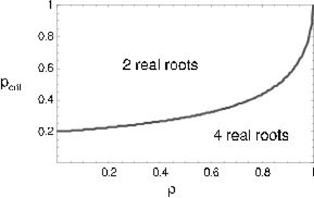
What is the nature of the roots ? Numerically, two situations occur when 0p10𝑝10\leq p\leq 1 and 0ρ10𝜌10\leq\rho\leq 1: there are either (i) four real roots or (ii) two real roots and two complex roots. For instance, when ρ=0.9𝜌0.9\rho=0.9, there are four real roots if p<0.5533938𝑝0.5533938p<0.5533938..., but only two otherwise. The separation of the two domains occurs when one root is degenerate. When this happens, the equalities Pcarac(BC)(p,ρ;x)=0superscriptsubscript𝑃caracBC𝑝𝜌𝑥0P_{\rm carac}^{\rm(BC)}(p,\rho;x)=0 and Pcarac(BC)(p,ρ;x)x=0superscriptsubscript𝑃caracBC𝑝𝜌𝑥𝑥0\displaystyle\frac{\partial P_{\rm carac}^{\rm(BC)}(p,\rho;x)}{\partial x}=0 lead to a polynomial constraint satisfied by p𝑝p and ρ𝜌\rho, given in the appendix (eq. (86)). For a given ρ𝜌\rho, there exists a unique solution in the range 0<p<10𝑝10<p<1, pcrit(ρ)subscript𝑝crit𝜌p_{\rm crit}(\rho), which is displayed in Fig. 6.


Refer to caption
Figure 6: Separation of the domains (ρ,p)𝜌𝑝(\rho,p) for which four real roots exist (under the curve) or two real and two complex roots coexist (above it).

From the inspection of eq. (35), we may wonder when numerator and denominator of the generating function may share a common root. A Gröbner basis calculation shows that this happens only when p=2𝑝2p=2, outside our range of interest. Therefore, there are four distinct roots most of the times, and when there is a double (real) root of 𝒫(pcrit(ρ),ρ;x)𝒫subscript𝑝crit𝜌𝜌𝑥{\mathcal{P}}(p_{\rm crit}(\rho),\rho;x), it is indeed degenerate (there is no simplification of GBC(z)subscript𝐺BC𝑧G_{\rm BC}(z)). The exact expression for Rel2(S0Sn)subscriptRel2subscript𝑆0subscript𝑆𝑛{\rm Rel}_{2}(S_{0}\rightarrow S_{n}) can then be deduced using a partial fraction decomposition of GBC(z)subscript𝐺BC𝑧G_{\rm BC}(z). When all the eigenvalues λisubscript𝜆𝑖\lambda_{i} are distinct,

GBC(z)=λiλiNBC(1λi)DBC(1λi)αi11λiz;subscript𝐺BC𝑧subscriptsubscript𝜆𝑖subscriptsubscript𝜆𝑖subscript𝑁BC1subscript𝜆𝑖subscriptsuperscript𝐷BC1subscript𝜆𝑖subscript𝛼𝑖11subscript𝜆𝑖𝑧G_{\rm BC}(z)=\sum_{\lambda_{i}}\;\underbrace{\frac{-\lambda_{i}\,N_{\rm BC}(\frac{1}{\lambda_{i}})}{D^{\prime}_{\rm BC}(\frac{1}{\lambda_{i}})}}_{\textstyle\alpha_{i}}\;\frac{1}{1-\lambda_{i}\,z}; (36)

consequently, the two-terminal reliability reads

Rel2(S0Sn)=λiαiλin.subscriptRel2subscript𝑆0subscript𝑆𝑛subscriptsubscript𝜆𝑖subscript𝛼𝑖superscriptsubscript𝜆𝑖𝑛{\rm Rel}_{2}(S_{0}\rightarrow S_{n})=\sum_{\lambda_{i}}\;\alpha_{i}\;\lambda_{i}^{n}. (37)

In the Brecht-Colbourn case, the root λmaxsubscript𝜆max\lambda_{\rm max} of greatest modulus is always real. Unless p𝑝p and ρ𝜌\rho are equal to 1, λmax<1subscript𝜆max1\lambda_{\rm max}<1, so that Rel2(BC)(S0Sn)superscriptsubscriptRel2BCsubscript𝑆0subscript𝑆𝑛{\rm Rel}_{2}^{({\rm BC})}(S_{0}\rightarrow S_{n}) decreases as n𝑛n\rightarrow\infty, essentially as a power-law behavior

Rel2(BC)(S0Sn)λmaxn.similar-tosuperscriptsubscriptRel2BCsubscript𝑆0subscript𝑆𝑛superscriptsubscript𝜆max𝑛{\rm Rel}_{2}^{({\rm BC})}(S_{0}\rightarrow S_{n})\sim\lambda_{\rm max}^{n}. (38)

4.2.2 Imperfect edges and perfect nodes

We devote this section to the case of imperfect edges and perfect nodes, since the Brecht-Colbourn ladder was initially investigated in this configuration [13, 14]. We immediately find

Rel2(BC;ρ=1)(S0Sn)=(0 1 0)(p21p2ppp2p2pp(12p))n(010),superscriptsubscriptRel2BC𝜌1subscript𝑆0subscript𝑆𝑛010superscriptsuperscript𝑝21superscript𝑝2missing-subexpressionmissing-subexpressionmissing-subexpression𝑝𝑝superscript𝑝2missing-subexpressionmissing-subexpressionmissing-subexpressionsuperscript𝑝2𝑝𝑝12𝑝𝑛010{\rm Rel}_{2}^{({\rm BC};\rho=1)}(S_{0}\rightarrow S_{n})=(0\;1\;0)\;\cdot\;\left(\begin{array}[]{c|c|c}p^{2}&1&p^{2}\\ \hline\cr p&p&p^{2}\\ \hline\cr-p^{2}&-p&p\,(1-2\,p)\end{array}\right)^{n}\;\cdot\;\left(\begin{array}[]{c}0\\ 1\\ 0\end{array}\right), (39)

so that the 25-node case [14] leads to

Rel2(S0S24)subscriptRel2subscript𝑆0subscript𝑆24\displaystyle{\rm Rel}_{2}(S_{0}\rightarrow S_{24}) =\displaystyle= p12(1+78p+1121p2+6633p3+11554p457525p5\displaystyle p^{12}\,\big{(}1+78\,p+1121\,p^{2}+6633\,p^{3}+11554\,p^{4}-57525\,p^{5} (40)
279450p6+89578p7+2570040p8+1431183p9279450superscript𝑝689578superscript𝑝72570040superscript𝑝81431183superscript𝑝9\displaystyle\hskip 28.45274pt-279450\,p^{6}+89578\,p^{7}+2570040\,p^{8}+1431183\,p^{9}
17159566p1012166498p11+98985590p1217159566superscript𝑝1012166498superscript𝑝1198985590superscript𝑝12\displaystyle\hskip 28.45274pt-17159566\,p^{10}-12166498\,p^{11}+98985590\,p^{12}
+33119917p13495566666p14+212008622p1533119917superscript𝑝13495566666superscript𝑝14212008622superscript𝑝15\displaystyle\hskip 28.45274pt+33119917\,p^{13}-495566666\,p^{14}+212008622\,p^{15}
+1867178285p162888906214p173066846055p181867178285superscript𝑝162888906214superscript𝑝173066846055superscript𝑝18\displaystyle\hskip 28.45274pt+1867178285\,p^{16}-2888906214\,p^{17}-3066846055\,p^{18}
+14427083319p1914178781875p2017955754991p2114427083319superscript𝑝1914178781875superscript𝑝2017955754991superscript𝑝21\displaystyle\hskip 28.45274pt+14427083319\,p^{19}-14178781875\,p^{20}-17955754991\,p^{21}
+80808979717p22144754404751p23+174732303288p2480808979717superscript𝑝22144754404751superscript𝑝23174732303288superscript𝑝24\displaystyle\hskip 28.45274pt+80808979717\,p^{22}-144754404751\,p^{23}+174732303288\,p^{24}
158925117297p25+113702258108p2665190712312p27158925117297superscript𝑝25113702258108superscript𝑝2665190712312superscript𝑝27\displaystyle\hskip 28.45274pt-158925117297\,p^{25}+113702258108\,p^{26}-65190712312\,p^{27}
+30133254848p2811197537798p29+3308571601p3030133254848superscript𝑝2811197537798superscript𝑝293308571601superscript𝑝30\displaystyle\hskip 28.45274pt+30133254848\,p^{28}-11197537798\,p^{29}+3308571601\,p^{30}
761406139p31+131805146p3216170009p33761406139superscript𝑝31131805146superscript𝑝3216170009superscript𝑝33\displaystyle\hskip 28.45274pt-761406139\,p^{31}+131805146\,p^{32}-16170009\,p^{33}
+1254886p3446368p35).\displaystyle\hskip 28.45274pt+1254886\,p^{34}-46368\,p^{35}\big{)}.

The coefficients are already quite large, even though the number of nodes remains limited. To the best of our knowledge, the exact two-terminal reliability polynomial was calculated only for a 10-node ladder [13]; we recover this result by taking n=9𝑛9n=9 in eq. (39).

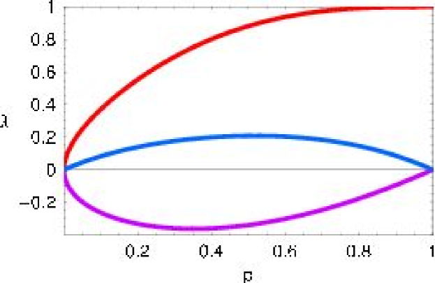
The three distinct real eigenvalues λisubscript𝜆𝑖\lambda_{i} (i=1,2,3𝑖123i=1,2,3) of the transfer matrix appearing in eq. (39), one of which is negative, are displayed as a function of p𝑝p in Fig. 7.

Refer to caption
Figure 7: Variation with p𝑝p of the three eigenvalues for the Brecht-Colbourn ladder with perfect nodes (see eq. (41)).

Their analytical expression is (ξ{1,e2iπ/3,e2iπ/3}𝜉1superscript𝑒2𝑖𝜋3superscript𝑒2𝑖𝜋3\xi\in\{1,e^{2\,i\,\pi/3},e^{-2\,i\,\pi/3}\})

λ=13p(2p)+13[ξ(𝒜+i272)1/3+ξ(𝒜i272)1/3],𝜆13𝑝2𝑝13delimited-[]𝜉superscript𝒜𝑖27213superscript𝜉superscript𝒜𝑖27213\lambda=\frac{1}{3}\,p\,(2-p)+\frac{1}{3}\;\left[\xi\,\left(\frac{{\mathcal{A}}+i\,\sqrt{27}\,\sqrt{{\mathcal{B}}}}{2}\right)^{1/3}+\xi^{*}\,\left(\frac{{\mathcal{A}}-i\,\sqrt{27}\,\sqrt{{\mathcal{B}}}}{2}\right)^{1/3}\right], (41)

where

𝒜𝒜\displaystyle{\mathcal{A}} =\displaystyle= p2(943p+60p239p3+11p4),superscript𝑝2943𝑝60superscript𝑝239superscript𝑝311superscript𝑝4\displaystyle-p^{2}\,\left(9-43\,p+60\,p^{2}-39\,p^{3}+11\,p^{4}\right), (42)
\displaystyle{\mathcal{B}} =\displaystyle= (1p)2p3(4+9p+16p288p3+98p432p58p6+5p7);superscript1𝑝2superscript𝑝349𝑝16superscript𝑝288superscript𝑝398superscript𝑝432superscript𝑝58superscript𝑝65superscript𝑝7\displaystyle{\left(1-p\right)}^{2}\,p^{3}\,\left(4+9\,p+16\,p^{2}-88\,p^{3}+98\,p^{4}-32\,p^{5}-8\,p^{6}+5\,p^{7}\right); (43)

note that {\mathcal{B}} is always positive for 0<p<10𝑝10<p<1.

The generating function for the Brecht-Colbourn ladder with perfect nodes is simply

GBC(ρ=1)(z)=1p(1p)z+p3(1p)z21p(2p)zp(1p)2(1+p)z2+p2(1p)2z3.superscriptsubscript𝐺BC𝜌1𝑧1𝑝1𝑝𝑧superscript𝑝31𝑝superscript𝑧21𝑝2𝑝𝑧𝑝superscript1𝑝21𝑝superscript𝑧2superscript𝑝2superscript1𝑝2superscript𝑧3G_{\rm BC}^{(\rho=1)}(z)=\frac{1-p\,(1-p)\,z+p^{3}\,(1-p)\,z^{2}}{1-p\,(2-p)\,z-p\,(1-p)^{2}\,(1+p)\,z^{2}+p^{2}\,(1-p)^{2}\,z^{3}}. (44)

From its partial fraction decomposition, which is necessarily of the form GBC(ρ=1)(z)=i=13αi1λizsuperscriptsubscript𝐺BC𝜌1𝑧superscriptsubscript𝑖13subscript𝛼𝑖1subscript𝜆𝑖𝑧G_{\rm BC}^{(\rho=1)}(z)=\displaystyle\sum_{i=1}^{3}\,\frac{\alpha_{i}}{1-\lambda_{i}\,z} because the eigenvalues are distinct, we deduce after simplification

Rel2(S0Sn)=i=13p(1p)2(1p)λiλi23p(1p)22(1p)2(1+p)λi(2p)λi2αiλin.subscriptRel2subscript𝑆0subscript𝑆𝑛superscriptsubscript𝑖13subscript𝑝superscript1𝑝21𝑝subscript𝜆𝑖superscriptsubscript𝜆𝑖23𝑝superscript1𝑝22superscript1𝑝21𝑝subscript𝜆𝑖2𝑝superscriptsubscript𝜆𝑖2subscript𝛼𝑖superscriptsubscript𝜆𝑖𝑛{\rm Rel}_{2}(S_{0}\rightarrow S_{n})=\sum_{i=1}^{3}\,\underbrace{\frac{p\,(1-p)^{2}-(1-p)\,\lambda_{i}-\lambda_{i}^{2}}{3\,p\,(1-p)^{2}-2(1-p)^{2}\,(1+p)\,\lambda_{i}-(2-p)\,\lambda_{i}^{2}}}_{\textstyle\alpha_{i}}\;\lambda_{i}^{n}. (45)

From eq. (45), it is clear that the large n𝑛n limit of Rel2(S0Sn)subscriptRel2subscript𝑆0subscript𝑆𝑛{\rm Rel}_{2}(S_{0}\rightarrow S_{n}) is a power-law behavior, in which the eigenvalue of maximum modulus quickly prevails over the others when p𝑝p is close to unity, even for moderate values of n𝑛n.

Table 1: Values of the Fisubscript𝐹𝑖F_{i}’s for the two-terminal reliability polynomial of the 25-node Brecht-Colbourn ladder.
i𝑖i Fisubscript𝐹𝑖F_{i} i𝑖i Fisubscript𝐹𝑖F_{i} i𝑖i Fisubscript𝐹𝑖F_{i} i𝑖i Fisubscript𝐹𝑖F_{i}
0 1 9 1125395882 18 762855455898 27 3042073238
1 47 10 3974128827 19 800820887863 28 635100751
2 1079 11 12199394435 20 725278875430 29 105465538
3 16103 12 32708854487 21 562806091836 30 13648753
4 175418 13 76833130394 22 371300292894 31 1334810
5 1484837 14 158368734141 23 206539411448 32 93929
6 10151340 15 286502593795 24 96061397122 33 4368
7 57524387 16 454444238576 25 37052347922 34 113
8 275139029 17 630595957484 26 11756780232 35 1

We can also write Rel2(S0Sn)=i=02n1Fip2n1i(1p)isubscriptRel2subscript𝑆0subscript𝑆𝑛superscriptsubscript𝑖02𝑛1subscript𝐹𝑖superscript𝑝2𝑛1𝑖superscript1𝑝𝑖\displaystyle{\rm Rel}_{2}(S_{0}\rightarrow S_{n})=\sum_{i=0}^{2\,n-1}\,F_{i}\,p^{2\,n-1-i}\,(1-p)^{i}, a well-known expansion of reliability polynomials [26]. The Fisubscript𝐹𝑖F_{i}’s for the 25-node ladder are given in Table 1 (the maximum value was equal to 8078 in the 10-node ladder [13]). Let us call m=n+1𝑚𝑛1m=n+1 the number of nodes. Using linear regressions on the first values of Rel2(S0Sn)subscriptRel2subscript𝑆0subscript𝑆𝑛{\rm Rel}_{2}(S_{0}\rightarrow S_{n}), it is straightforward to find

Rel2(modd)(p)superscriptsubscriptRel2𝑚odd𝑝\displaystyle{\rm Rel}_{2}^{(m{\rm\ odd)}}(p) =\displaystyle= pm12(1p)3m52+m212m218pm+12(1p)3m72superscript𝑝𝑚12superscript1𝑝3𝑚52superscript𝑚212𝑚218superscript𝑝𝑚12superscript1𝑝3𝑚72\displaystyle p^{\frac{m-1}{2}}\,(1-p)^{\frac{3\,m-5}{2}}+\frac{m^{2}-12\,m-21}{8}\,p^{\frac{m+1}{2}}\,(1-p)^{\frac{3\,m-7}{2}} (46)
+m4+72m3+350m22376m+2337384pm+32(1p)3m92superscript𝑚472superscript𝑚3350superscript𝑚22376𝑚2337384superscript𝑝𝑚32superscript1𝑝3𝑚92\displaystyle\hskip-56.9055pt+\frac{m^{4}+72\,m^{3}+350\,m^{2}-2376\,m+2337}{384}\,p^{\frac{m+3}{2}}\,(1-p)^{\frac{3\,m-9}{2}}
+\displaystyle\hskip-56.9055pt+\cdots
Rel2(meven)(p)superscriptsubscriptRel2𝑚even𝑝\displaystyle{\rm Rel}_{2}^{(m{\rm\ even)}}(p) =\displaystyle= m2pm2(1p)3m62+(m2)(m2+38m+24)48pm+22(1p)3m82𝑚2superscript𝑝𝑚2superscript1𝑝3𝑚62𝑚2superscript𝑚238𝑚2448superscript𝑝𝑚22superscript1𝑝3𝑚82\displaystyle\frac{m}{2}\,p^{\frac{m}{2}}\,(1-p)^{\frac{3\,m-6}{2}}+\frac{(m-2)\,(m^{2}+38\,m+24)}{48}\,p^{\frac{m+2}{2}}\,(1-p)^{\frac{3\,m-8}{2}} (47)
+(m2)(m4+122m3+2304m25472m13440)3840pm+42(1p)3m102𝑚2superscript𝑚4122superscript𝑚32304superscript𝑚25472𝑚134403840superscript𝑝𝑚42superscript1𝑝3𝑚102\displaystyle\hskip-56.9055pt+\frac{(m-2)\,(m^{4}+122\,m^{3}+2304\,m^{2}-5472\,m-13440)}{3840}\,p^{\frac{m+4}{2}}\,(1-p)^{\frac{3\,m-10}{2}}
+\displaystyle\hskip-56.9055pt+\cdots

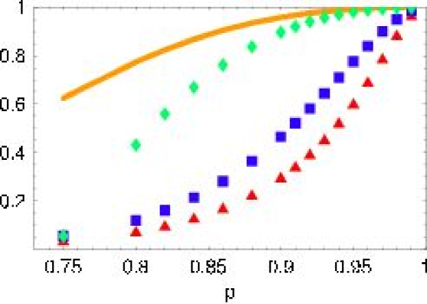
Finally, the comparison of the exact results with the various lower bounds proposed in [14] is given in Table 2 and Fig. 8. It shows that the lower bound of Brecht and Colbourn is rather good for p𝑝p close to unity, but its sharpness decreases for p<0.8𝑝0.8p<0.8.

Table 2: Comparison of various lower bounds with the exact two-terminal reliability of a 25-node Brecht-Colbourn ladder [14].
p𝑝p Kruskal-Katona MinCost(edp) Brecht-Colbourn exact
0.75 0.031682 0.054681 0.054681 0.625163
0.80 0.068803 0.119917 0.430912 0.773696
0.82 0.092654 0.161200 0.558991 0.824038
0.84 0.124041 0.214282 0.669269 0.867950
0.86 0.165305 0.281396 0.761945 0.905042
0.88 0.219694 0.364529 0.837486 0.935251
0.90 0.291856 0.464826 0.896659 0.958806
0.91 0.336579 0.521297 0.920440 0.968231
0.92 0.388392 0.581555 0.940574 0.976194
0.93 0.448415 0.644934 0.957259 0.982785
0.94 0.517724 0.710375 0.970720 0.988109
0.95 0.597041 0.776313 0.981207 0.992275
0.96 0.686113 0.840514 0.989003 0.995400
0.97 0.782518 0.899895 0.994420 0.997608
0.98 0.879474 0.950274 0.997801 0.999024
0.99 0.961964 0.986085 0.999524 0.999778
Refer to caption
Figure 8: Comparison of the exact value () with lower bounds given in ref. [14] for the 25-node ladder:(\blacktriangle) Kruskal-Katona (\blacksquare) Min Cost (\blacklozenge) Brecht-Colbourn.

4.2.3 Imperfect nodes and perfect edges

The configuration of imperfect nodes and perfect edges, although less studied than the previous one, has nonetheless been considered in several papers [1, 12, 35]. The Brecht-Colbourn ladder case has been studied in detail by Graver and Sobel [35]. The relevant transfer matrix is now equal to

M(p=1,ρ)=(00ρ0ρρ0ρ1ρρρρρρρ).𝑀𝑝1𝜌00𝜌0missing-subexpressionmissing-subexpressionmissing-subexpressionmissing-subexpression𝜌𝜌0𝜌missing-subexpressionmissing-subexpressionmissing-subexpressionmissing-subexpression1𝜌𝜌𝜌missing-subexpressionmissing-subexpressionmissing-subexpressionmissing-subexpression𝜌𝜌𝜌𝜌M(p=1,\rho)=\left(\begin{array}[]{l|l|l|l}0&0&\rho&0\\ \hline\cr\rho&\rho&0&\rho\\ \hline\cr 1&\rho&\rho&\rho\\ \hline\cr-\rho&-\rho&-\rho&-\rho\end{array}\right). (48)

Its characteristic polynomial is x2(x2ρxρ(1ρ))superscript𝑥2superscript𝑥2𝜌𝑥𝜌1𝜌x^{2}\,(x^{2}-\rho\,x-\rho\,(1-\rho)), which simply leads to the eigenvalues 0 — which plays no role in the final expression of the two-terminal reliability — and λ±=12(ρ±4ρ3ρ2)subscript𝜆plus-or-minus12plus-or-minus𝜌4𝜌3superscript𝜌2\displaystyle\lambda_{\pm}=\frac{1}{2}\,\left(\rho\pm\sqrt{4\,\rho-3\,\rho^{2}}\right). The generating function is found to be

GBC(p=1)(z)=ρ1ρzρ(1ρ)z2=ρλ+λ(λ+1λ+zλ1λz),superscriptsubscript𝐺BC𝑝1𝑧𝜌1𝜌𝑧𝜌1𝜌superscript𝑧2𝜌subscript𝜆subscript𝜆subscript𝜆1subscript𝜆𝑧subscript𝜆1subscript𝜆𝑧G_{{\rm BC}}^{(p=1)}(z)=\frac{\rho}{1-\rho\,z-\rho\,(1-\rho)\,z^{2}}=\frac{\rho}{\lambda_{+}-\lambda_{-}}\,\left(\frac{\lambda_{+}}{1-\lambda_{+}\,z}-\frac{\lambda_{-}}{1-\lambda_{-}\,z}\right), (49)

which gives

Rel2(S0Sn)=ρ4ρ3ρ2(λ+n+1λn+1).subscriptRel2subscript𝑆0subscript𝑆𝑛𝜌4𝜌3superscript𝜌2superscriptsubscript𝜆𝑛1superscriptsubscript𝜆𝑛1{\rm Rel}_{2}(S_{0}\rightarrow S_{n})=\frac{\rho}{\sqrt{4\,\rho-3\,\rho^{2}}}\,\left(\lambda_{+}^{n+1}-\lambda_{-}^{n+1}\right). (50)

This is almost Graver and Sobel’s result [35], obtained through a combinatorial argument. Their final expression differs from ours because their source and destination (in our notation, S0subscript𝑆0S_{0} and Snsubscript𝑆𝑛S_{n}) are perfect.

4.3 Generalized fan

When the reliabilities are p𝑝p et ρ𝜌\rho, the transfer matrix of eq. (23) is equal to

M^(p,ρ)=(pρ0000pρpρp2ρp2ρp2ρ1p2ρp2ρp2ρpρp(12p)ρ)^𝑀𝑝𝜌𝑝𝜌000missing-subexpressionmissing-subexpressionmissing-subexpressionmissing-subexpression0𝑝𝜌𝑝𝜌superscript𝑝2𝜌missing-subexpressionmissing-subexpressionmissing-subexpressionmissing-subexpressionsuperscript𝑝2𝜌superscript𝑝2𝜌1superscript𝑝2𝜌missing-subexpressionmissing-subexpressionmissing-subexpressionmissing-subexpressionsuperscript𝑝2𝜌superscript𝑝2𝜌𝑝𝜌𝑝12𝑝𝜌\widehat{M}(p,\rho)=\left(\begin{array}[]{l|l|l|l}p\,\rho&0&0&0\\ \hline\cr 0&p\,\rho&p\,\rho&p^{2}\,\rho\\ \hline\cr p^{2}\,\rho&p^{2}\,\rho&1&p^{2}\,\rho\\ \hline\cr-p^{2}\,\rho&-p^{2}\,\rho&-p\,\rho&p\,(1-2\,p)\,\rho\end{array}\right) (51)

and

Rel2(S0Sn)=1p(1ρ 0 0)M^(p,ρ)n+1(1000),subscriptRel2subscript𝑆0subscript𝑆𝑛1𝑝1𝜌00^𝑀superscript𝑝𝜌𝑛11000{\rm Rel}_{2}(S_{0}\rightarrow S_{n})=\frac{1}{p}\,(1\;\rho\;0\;0)\,\cdot\,\widehat{M}(p,\rho)^{n+1}\,\cdot\,\left(\begin{array}[]{c}1\\ 0\\ 0\\ 0\end{array}\right), (52)

the 1/p1𝑝1/p prefactor being a consequence of the condition a01subscript𝑎01a_{0}\equiv 1 in M^0subscript^𝑀0\widehat{M}_{0}. The characteristic polynomial of this matrix factorizes nicely:

Pcarac(fan)(p,ρ;x)=(x1)(xpρ)(xp(1p)ρ)2,superscriptsubscript𝑃caracfan𝑝𝜌𝑥𝑥1𝑥𝑝𝜌superscript𝑥𝑝1𝑝𝜌2P_{{\rm carac}}^{\rm(fan)}(p,\rho;x)=(x-1)\,(x-p\,\rho)\,\bigg{(}x-p\,(1-p)\,\rho\bigg{)}^{2}, (53)

so that the eigenvalues are 1, pρ𝑝𝜌p\,\rho and p(1p)ρ𝑝1𝑝𝜌p\,(1-p)\,\rho, the latter being of degree 2. The presence of 1 among the roots should not be surprising. Indeed, even when n𝑛n goes to infinity, the two-terminal reliability between S0subscript𝑆0S_{0} and Snsubscript𝑆𝑛S_{n} is larger than pρ2𝑝superscript𝜌2p\,\rho^{2}, in stark contrast to the Brecht-Colbourn case, where the reliability vanishes. Since a power-law behavior is still expected, the only possibility is that the largest eigenvalue is of modulus 1.

The generating function G(fan)(z)superscript𝐺fan𝑧G^{({\rm fan})}(z) is derived using the recipe described in the Brecht-Colbourn case. The additional convention Rel2(S0S0)=ρsubscriptRel2subscript𝑆0subscript𝑆0𝜌{\rm Rel}_{2}(S_{0}\rightarrow S_{0})=\rho leads to

G(fan)(z)superscript𝐺fan𝑧\displaystyle G^{({\rm fan})}(z) =\displaystyle= N(fan)(z)D(fan)(z),superscript𝑁fan𝑧superscript𝐷fan𝑧\displaystyle\frac{N^{({\rm fan})}(z)}{D^{({\rm fan})}(z)}, (54)
N(fan)(z)superscript𝑁fan𝑧\displaystyle N^{({\rm fan})}(z) =\displaystyle= 1z[1+pρ(1p)(2pρ)]+pρz2[(2+pρ)(1p)\displaystyle 1-z\,\big{[}1+p\,\rho\,(1-p)\,(2-p\,\rho)\big{]}+p\,\rho\,z^{2}\,\big{[}(2+p\rho)\,(1-p) (55)
+p2ρ(pρ)]p2(1p)2ρ2z3,\displaystyle+p^{2}\,\rho\,(p-\rho)\big{]}-p^{2}\,(1-p)^{2}\,\rho^{2}\,z^{3},
D(fan)(z)superscript𝐷fan𝑧\displaystyle D^{({\rm fan})}(z) =\displaystyle= (1z)(1pρz)(1p(1p)ρz)2.1𝑧1𝑝𝜌𝑧superscript1𝑝1𝑝𝜌𝑧2\displaystyle(1-z)\,(1-p\,\rho\,z)\,\big{(}1-p\,(1-p)\,\rho\,z\big{)}^{2}. (56)

Because all the roots have simple expressions, we expect to find a simple, analytical expression for Rel2(fan)(S0Sn)superscriptsubscriptRel2fansubscript𝑆0subscript𝑆𝑛{\rm Rel}_{2}^{({\rm fan})}(S_{0}\rightarrow S_{n}). The partial fraction decomposition of eq. (54) gives indeed

G(fan)(z)superscript𝐺fan𝑧\displaystyle G^{({\rm fan})}(z) =\displaystyle= ρ2(1p)(1p(1p)ρ)212p(1p)ρ+p2ρ2(13p+p2)1p(1p)ρzsuperscript𝜌21𝑝superscript1𝑝1𝑝𝜌212𝑝1𝑝𝜌superscript𝑝2superscript𝜌213𝑝superscript𝑝21𝑝1𝑝𝜌𝑧\displaystyle\frac{\rho^{2}\,(1-p)}{\big{(}1-p\,(1-p)\,\rho\big{)}^{2}}\,\frac{1-2\,p\,(1-p)\,\rho+p^{2}\,\rho^{2}\,(1-3\,p+p^{2})}{1-p\,(1-p)\,\rho\,z} (57)
+pρ21pρ(2p)1p(1p)ρ1(1p(1p)ρz)2𝑝superscript𝜌21𝑝𝜌2𝑝1𝑝1𝑝𝜌1superscript1𝑝1𝑝𝜌𝑧2\displaystyle+p\,\rho^{2}\,\frac{1-p\,\rho\,(2-p)}{1-p\,(1-p)\,\rho}\;\frac{1}{(1-p\,(1-p)\,\rho\,z)^{2}}
+p2ρ3(1p(1p)ρ)211z+ρ(1ρ)11pρz.superscript𝑝2superscript𝜌3superscript1𝑝1𝑝𝜌211𝑧𝜌1𝜌11𝑝𝜌𝑧\displaystyle+\frac{p^{2}\,\rho^{3}}{\big{(}1-p\,(1-p)\,\rho\big{)}^{2}}\;\frac{1}{1-z}+\rho\,(1-\rho)\,\frac{1}{1-p\,\rho\,z}.

The new feature of eq. (57) is the (1p(1p)ρz)2superscript1𝑝1𝑝𝜌𝑧2(1-p\,(1-p)\,\rho\,z)^{-2} term. Because

1(1λz)2=n=0(n+1)λnzn,1superscript1𝜆𝑧2superscriptsubscript𝑛0𝑛1superscript𝜆𝑛superscript𝑧𝑛\frac{1}{(1-\lambda\,z)^{2}}=\sum_{n=0}^{\infty}\,(n+1)\,\lambda^{n}\,z^{n}, (58)

the final expression of the two-terminal reliability is

Rel2(fan)(S0Sn)superscriptsubscriptRel2fansubscript𝑆0subscript𝑆𝑛\displaystyle{\rm Rel}_{2}^{\rm(fan)}(S_{0}\rightarrow S_{n}) =\displaystyle= +pn(1p)nρn+2(np1pρ(2p)1p(1p)ρ\displaystyle+p^{n}\,(1-p)^{n}\,\rho^{n+2}\,\left(n\,p\,\frac{1-p\,\rho\,(2-p)}{1-p\,(1-p)\,\rho}\right. (59)
+1pρ(2p)+p2(1p)2ρ2(1p(1p)ρ)2)\displaystyle\hskip 56.9055pt\left.+\frac{1-p\,\rho\,(2-p)+p^{2}\,(1-p)^{2}\,\rho^{2}}{\big{(}1-p\,(1-p)\,\rho\big{)}^{2}}\right)
+pnρn+1(1ρ)+p2ρ3(1p(1p)ρ)2,superscript𝑝𝑛superscript𝜌𝑛11𝜌superscript𝑝2superscript𝜌3superscript1𝑝1𝑝𝜌2\displaystyle+p^{n}\,\rho^{n+1}\,(1-\rho)+\frac{p^{2}\,\rho^{3}}{\big{(}1-p\,(1-p)\,\rho\big{)}^{2}},

where n𝑛n appears in a prefactor, not only as an exponent. The second term of eq. (59) is the asymptotic limit when n𝑛n\rightarrow\infty. We see that the reliability of the path S0TSnsubscript𝑆0𝑇subscript𝑆𝑛S_{0}\rightarrow T\rightarrow S_{n} is enhanced by 1/(1p(1p)ρ)21superscript1𝑝1𝑝𝜌21/\big{(}1-p\,(1-p)\,\rho\big{)}^{2}. When nodes are perfect, ρ𝜌\rho must be set to one in eq. (59), and the contribution of the eigenvalue pρ𝑝𝜌p\,\rho vanishes (the transfer matrix of eq. (27) is 3×3333\times 3). This leads to

Rel2(fan;ρ=1)(S0Sn)superscriptsubscriptRel2fan𝜌1subscript𝑆0subscript𝑆𝑛\displaystyle{\rm Rel}_{2}^{({\rm fan};\rho=1)}(S_{0}\rightarrow S_{n}) =\displaystyle= pn(1p)n+2(np1p(1p)+(1+p2)(1p(1p))2)superscript𝑝𝑛superscript1𝑝𝑛2𝑛𝑝1𝑝1𝑝1superscript𝑝2superscript1𝑝1𝑝2\displaystyle p^{n}\,(1-p)^{n+2}\,\left(\frac{n\,p}{1-p\,(1-p)}+\frac{(1+p^{2})}{\big{(}1-p\,(1-p)\big{)}^{2}}\right) (60)
+p2(1p(1p))2.superscript𝑝2superscript1𝑝1𝑝2\displaystyle+\frac{p^{2}}{\big{(}1-p\,(1-p)\big{)}^{2}}.

5 Zeros of the two-terminal reliability polynomials

The structure of the different reliability polynomials may be understood by studying the locations of their zeros in the complex plane. Such a study has been fruitfully performed in the case of the chromatic polynomial [9, 11, 57], most notably in the context of the four-color theorem. In reliability studies, some effort has been done to discover general properties for the all-terminal reliability RelA(p)subscriptRel𝐴𝑝{\rm Rel}_{A}(p) [21, 28, 51], its main byproduct being the Brown-Colbourn conjecture [16], according to which all the zeros are to be found in the region |1p|<11𝑝1|1-p|<1. Although valid for series-parallel graphs, this remarkable conjecture does not strictly hold in the general case (but not by far) [56]. As mentioned in the introduction, the all-reliability polynomial is linked to the Tutte polynomial, an invariant of the graph. It has also been studied extensively by Chang and Shrock for various recursive families of graphs [19], who give the limiting curves where all zeros of the polynomials converge.

In this section, after briefly recalling general results of the literature, we study the roots of Rel2(p,ρ)=0subscriptRel2𝑝𝜌0{\rm Rel}_{2}(p,\rho)=0 in the complex plane for a fixed ρ𝜌\rho, in order to see whether some insight may also be gained in this case. Admittedly, this polynomial depends on the couple (source, terminal), but structures are still expected. We show that the zeros tend to aggregate along portions of algebraic curves, which can substantially differ even for the two families of graphs under consideration, even though they have the same all-terminal reliability. Moreover, structural transitions occur at ρ=12𝜌12\rho=\frac{1}{2}.

5.1 Calculation of the limiting curves (generalities)

As n𝑛n grows, the number of zeros of the reliability polynomial in the complex plane increases. Because of the matrix transfer property, we have recursion relations between relability polynomials corresponding to successive values of n𝑛n. The general treatment of the problem has been done by Beraha, Kahane, and Weiss [8], but may be understood in the following, simplifying way: if the reliability polynomial is of the form iαiλi(p)nsubscript𝑖subscript𝛼𝑖subscript𝜆𝑖superscript𝑝𝑛\sum_{i}\alpha_{i}\,\lambda_{i}(p)^{n} (where λisubscript𝜆𝑖\lambda_{i} are the eigenvalues of the transfer matrix), then at large n𝑛n, only the two eigenvalues of greater modules, say λ1subscript𝜆1\lambda_{1} and λ2subscript𝜆2\lambda_{2}, will prevail, so that the reliability polynomial will vanish when |λ1(p)|=|λ2(p)|subscript𝜆1𝑝subscript𝜆2𝑝|\lambda_{1}(p)|=|\lambda_{2}(p)| (of course, it might be three or more eigenvalues of equal modulus; the present oversimplification works quite well here). This defines a set of curves in the complex plane, where all zeros should accumulate in the n𝑛n\rightarrow\infty limit. The interested reader should refer to the work of Salas and Sokal [57] for a very detailed discussion of the convergence to the limiting curves. This behavior is not modified when one or more of the αisubscript𝛼𝑖\alpha_{i}’s is a polynomial in n𝑛n [8], as will become apparent for the generalized fan.

5.2 Calculation for the Brecht-Colbourn ladder

The recursion relation obeyed by Rel2(BC)(S0Sn)Rel2(n)superscriptsubscriptRel2BCsubscript𝑆0subscript𝑆𝑛superscriptsubscriptRel2𝑛{\rm Rel}_{2}^{({\rm BC})}(S_{0}\rightarrow S_{n})\equiv{\rm Rel}_{2}^{(n)} is easily deduced from eq. (31); it reads

Rel2(n)(p)superscriptsubscriptRel2𝑛𝑝\displaystyle{\rm Rel}_{2}^{(n)}(p) =\displaystyle= p(2p)ρRel2(n1)+pρ(1pρp2ρ+p3ρ)Rel2(n2)𝑝2𝑝𝜌superscriptsubscriptRel2𝑛1𝑝𝜌1𝑝𝜌superscript𝑝2𝜌superscript𝑝3𝜌superscriptsubscriptRel2𝑛2\displaystyle p\,(2-p)\,\rho\,{\rm Rel}_{2}^{(n-1)}+p\,\rho\,(1-p\,\rho-p^{2}\,\rho+p^{3}\,\rho)\,{\rm Rel}_{2}^{(n-2)} (61)
p2(1p)ρ2(1ρ)Rel2(n3)+p4(1p)ρ3(1ρ)Rel2(n4).superscript𝑝21𝑝superscript𝜌21𝜌superscriptsubscriptRel2𝑛3superscript𝑝41𝑝superscript𝜌31𝜌superscriptsubscriptRel2𝑛4\displaystyle\hskip-28.45274pt-p^{2}\,(1-p)\,\rho^{2}\,(1-\rho)\,{\rm Rel}_{2}^{(n-3)}+p^{4}\,(1-p)\,\rho^{3}\,(1-\rho)\,{\rm Rel}_{2}^{(n-4)}.

and leads to very quick calculations using mathematical softwares such as Mathematica [45]. Note that this recursion relation of order four becomes of order three when ρ=1𝜌1\rho=1. We can then look for solutions of Rel2(n)(p)=0superscriptsubscriptRel2𝑛𝑝0{\rm Rel}_{2}^{(n)}(p)=0 in the complex plane. Of course, the degree of the polynomial, as well as the magnitude of its coefficients, will increase with n𝑛n.

5.2.1 Perfect nodes

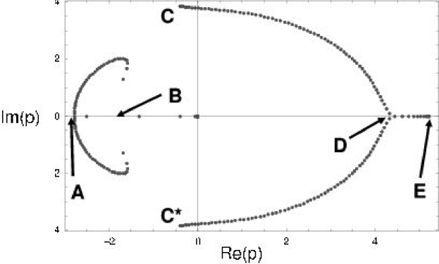
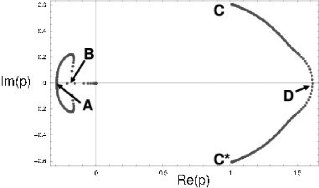
Let us begin by setting ρ=1𝜌1\rho=1. A first step is to display the roots of Rel2(n)(p)=0superscriptsubscriptRel2𝑛𝑝0{\rm Rel}_{2}^{(n)}(p)=0. These zeros have been calculated using the NSolve[] routine of Mathematica; because the polynomial coefficients can be very large, a numerical accuracy of several hundred digits is sometimes necessary. Figure 9 shows the location of the zeros of Rel2(150)(p)superscriptsubscriptRel2150𝑝{\rm Rel}_{2}^{(150)}(p) in the complex plane (it corresponds to a graph with 151 nodes and 299 edges).
Refer to caption
Figure 9: Localization of the complex roots p𝑝p of the two-terminal reliability polynomial for a Brecht-Colbourn ladder of 151 perfect nodes and 299 edges.

On the right half of the complex plane, we have a simple, open curve crossing the real axis at D𝐷D and extremities at C𝐶C and Csuperscript𝐶C^{*}. On the left half, however, we have what looks like a closed curve — intersecting the negative real axis in A𝐴A and B𝐵B — as well as some dots on the negative real axis, between A𝐴A and the origin.

As mentioned above, it is well known that as n𝑛n increases, the zeros accumulate at particular locations, constituted by segments/portions of algebraic curves. For n=150𝑛150n=150, these limits are almost reached, even though the “sampling” is not uniform. We can calculate the limiting curves by considering that the roots of the characteristic polynomial are λeiθ/2𝜆superscript𝑒𝑖𝜃2\lambda\,e^{i\,\theta/2}, λeiθ/2𝜆superscript𝑒𝑖𝜃2\lambda\,e^{-i\,\theta/2} and μ𝜇\mu. The coefficients of the characteristic polynomial imply constraints between λ𝜆\lambda (which may be complex), μ𝜇\mu and θ𝜃\theta, or more precisely, t=cosθ2𝑡𝜃2t=\cos\frac{\theta}{2} or T=cosθ𝑇𝜃T=\cos\theta, which will be used in the following. For instance, μ=(2p)p2λcosθ2𝜇2𝑝𝑝2𝜆𝜃2\mu=(2-p)\,p-2\,\lambda\,\cos\frac{\theta}{2}. After eliminating λ𝜆\lambda and μ𝜇\mu, we obtain a compatibility condition which must be satisfied by p𝑝p, and T𝑇T (the polynomial 𝒫3(p,ρ,T)subscript𝒫3𝑝𝜌𝑇{\mathcal{P}}_{3}(p,\rho,T) is given in eq. (84)):

𝒫3(p,ρ=1,T)\displaystyle{\mathcal{P}}_{3}(p,\rho=1,T) =\displaystyle= 2+9p4p230p3+38p410p56p6+3p729𝑝4superscript𝑝230superscript𝑝338superscript𝑝410superscript𝑝56superscript𝑝63superscript𝑝7\displaystyle 2+9\,p-4\,p^{2}-30\,p^{3}+38\,p^{4}-10\,p^{5}-6p^{6}+3\,p^{7} (62)
+(2+12p8p234p3+48p418p52p6+2p7)T212𝑝8superscript𝑝234superscript𝑝348superscript𝑝418superscript𝑝52superscript𝑝62superscript𝑝7𝑇\displaystyle+\left(2+12\,p-8\,p^{2}-34\,p^{3}+48\,p^{4}-18\,p^{5}-2\,p^{6}+2\,p^{7}\right)\,T
4p(1p)2(1p+p2)T28p(1p)2T34𝑝superscript1𝑝21𝑝superscript𝑝2superscript𝑇28𝑝superscript1𝑝2superscript𝑇3\displaystyle-4\,p\,(1-p)^{2}\,\left(1-p+p^{2}\right)\,T^{2}-8\,p\,(1-p)^{2}\,T^{3}
=\displaystyle= 0.0\displaystyle 0.

The additional requirement |μ|<|λ|𝜇𝜆|\mu|<|\lambda| translates into an additional contraint between p𝑝p and T𝑇T.

A plot of this parametric set of curves shows indeed that the whole portion of the negative real axis between A𝐴A and the origin is indeed a solution, so that we could expect more zeros there when n>150𝑛150n>150.

A few critical points can also be deduced from eq. (62). For instance, D𝐷D corresponds to a real solution of 𝒫3(p,ρ=1,T=1)=0{\mathcal{P}}_{3}(p,\rho=1,T=-1)=0, namely pD=1+52subscript𝑝𝐷152p_{D}=\frac{1+\sqrt{5}}{2}. C𝐶C and Csuperscript𝐶C^{*} are points of the complex plane defined by pCsubscript𝑝𝐶p_{C} and its complex conjugate, which are roots of 𝒫3(p,ρ=1,T=+1)=0{\mathcal{P}}_{3}(p,\rho=1,T=+1)=0, that is

4+9p+16p288p3+98p432p58p6+5p7=0.49𝑝16superscript𝑝288superscript𝑝398superscript𝑝432superscript𝑝58superscript𝑝65superscript𝑝704+9\,p+16\,p^{2}-88\,p^{3}+98\,p^{4}-32\,p^{5}-8\,p^{6}+5\,p^{7}=0. (63)

This polynomial already appeared in the expression of {\mathcal{B}}. Note that there are more than one pair of complex solutions to this equation, the relevant one is given by pC1.011578+i 0.607394subscript𝑝𝐶1.011578𝑖0.607394p_{C}\approx 1.011578+i\,0.607394. The determination of the complex numbers pAsubscript𝑝𝐴p_{A} and pBsubscript𝑝𝐵p_{B} associated with A𝐴A and B𝐵B is a little more elaborate. Both pAsubscript𝑝𝐴p_{A} and pBsubscript𝑝𝐵p_{B} are real and negative; they correspond to roots of degree two of eq. (62). In order to find them, we must have 𝒫3(p,ρ=1,T)=0{\mathcal{P}}_{3}(p,\rho=1,T)=0 and 𝒫3(p,ρ=1,T)p=0\displaystyle\frac{\partial{\mathcal{P}}_{3}(p,\rho=1,T)}{\partial p}=0. These two relations are satisfied for special values of p𝑝p (or T𝑇T). After substitution and elimination of T𝑇T using Mathematica, we obtain a product of polynomials, which must cancel for p=pA𝑝subscript𝑝𝐴p=p_{A} and p=pB𝑝subscript𝑝𝐵p=p_{B}. For the sake of completeness, we provide the needed polynomials in appendix A. A close numerical study allows to identify the relevant polynomials:

  • pA0.2879878subscript𝑝𝐴0.2879878p_{A}\approx-0.2879878 is solution of 𝒫1(p,ρ=1)=0subscript𝒫1𝑝𝜌10{\mathcal{P}}_{1}(p,\rho=1)=0 (see eq. (82)), that is

    0=1p11p2+15p33p42p5p6+p7,01𝑝11superscript𝑝215superscript𝑝33superscript𝑝42superscript𝑝5superscript𝑝6superscript𝑝70=1-p-11\,p^{2}+15\,p^{3}-3\,p^{4}-2\,p^{5}-p^{6}+p^{7}, (64)

    attained for T0.138176𝑇0.138176T\approx 0.138176, a root of

    0=1+11T27T226T3+140T4+240T5+144T6+32T7.0111𝑇27superscript𝑇226superscript𝑇3140superscript𝑇4240superscript𝑇5144superscript𝑇632superscript𝑇70=-1+11\,T-27\,T^{2}-26\,T^{3}+140\,T^{4}+240\,T^{5}+144\,T^{6}+32\,T^{7}. (65)
  • pB0.1849482subscript𝑝𝐵0.1849482p_{B}\approx-0.1849482 is solution of 𝒫2(p,ρ=1)=0subscript𝒫2𝑝𝜌10{\mathcal{P}}_{2}(p,\rho=1)=0 (see eq. (83)), i.e.,

    00\displaystyle 0 =\displaystyle= 14p9p2+101p3413p4+1019p51761p614𝑝9superscript𝑝2101superscript𝑝3413superscript𝑝41019superscript𝑝51761superscript𝑝6\displaystyle 1-4\,p-9\,p^{2}+101\,p^{3}-413\,p^{4}+1019\,p^{5}-1761\,p^{6} (66)
    +2151p71864p8+1097p9386p10+60p11,2151superscript𝑝71864superscript𝑝81097superscript𝑝9386superscript𝑝1060superscript𝑝11\displaystyle+2151\,p^{7}-1864\,p^{8}+1097\,p^{9}-386\,p^{10}+60\,p^{11},

    attained for T0.9511957𝑇0.9511957T\approx-0.9511957, one of the solutions of

    00\displaystyle 0 =\displaystyle= 3040707+12576464T+15322821T24376828T3304070712576464𝑇15322821superscript𝑇24376828superscript𝑇3\displaystyle 3040707+12576464\,T+15322821\,T^{2}-4376828\,T^{3} (67)
    22559186T410112842T5+9510320T6+7762048T722559186superscript𝑇410112842superscript𝑇59510320superscript𝑇67762048superscript𝑇7\displaystyle-22559186\,T^{4}-10112842\,T^{5}+9510320\,T^{6}+7762048\,T^{7}
    1337920T82068608T9+8192T10+204800T111337920superscript𝑇82068608superscript𝑇98192superscript𝑇10204800superscript𝑇11\displaystyle-1337920\,T^{8}-2068608\,T^{9}+8192\,T^{10}+204800\,T^{11}

5.2.2 Imperfect nodes

We can perform the study for ρ<1𝜌1\rho<1 by following the same lines as above. Although more cumbersome because there are now four possible roots instead of three, the calculations are interesting nonetheless because we may vary one parameter, ρ𝜌\rho. A natural question is: can it affect the global structure of the zeros ? The answer is yes, and the location of the zeros undergoes a kind of “structural transition” for a particular value of ρ𝜌\rho, namely 1212\frac{1}{2}.

Let us first consider ρ>12𝜌12\rho>\frac{1}{2}. The location of the zeros is then qualitatively similar to that described in Fig. 9, the whole structure merely expanding from the origin. After comparison with the numerical values for n=150𝑛150n=150, D𝐷D appears to be associated with pD=12(1+1+4ρ)subscript𝑝𝐷12114𝜌p_{D}=\frac{1}{2}\,(1+\sqrt{1+\frac{4}{\rho}}), the relevant solution of 𝒫3(p,ρ,T=1)=0subscript𝒫3𝑝𝜌𝑇10{\mathcal{P}}_{3}(p,\rho,T=-1)=0. Likewise, C𝐶C and Csuperscript𝐶C^{*} are given by pCsubscript𝑝𝐶p_{C}, which is one complex solution of 𝒫3(p,ρ,T=+1)=0subscript𝒫3𝑝𝜌𝑇10{\mathcal{P}}_{3}(p,\rho,T=+1)=0 (𝒫3subscript𝒫3{\mathcal{P}}_{3} is given in eq. (84)).

The determination of pAsubscript𝑝𝐴p_{A} and pBsubscript𝑝𝐵p_{B} is more tedious, because 𝒫3(p,ρ,T)subscript𝒫3𝑝𝜌𝑇{\mathcal{P}}_{3}(p,\rho,T) is now a polynomial of degree 6 in T𝑇T. Here again, we must find the common zeros of 𝒫3(p,ρ,T)subscript𝒫3𝑝𝜌𝑇{\mathcal{P}}_{3}(p,\rho,T) and its derivative with respect to p𝑝p. The elimination of T𝑇T, performed using Mathematica, leads to a polynomial in p𝑝p and ρ𝜌\rho, which must vanish. Actually, this polynomial can be factored, and a numerical comparison with the zeros obtained for n=150𝑛150n=150 shows that pAsubscript𝑝𝐴p_{A} is solution of 𝒫1(p,ρ)=0subscript𝒫1𝑝𝜌0{\mathcal{P}}_{1}(p,\rho)=0 (see eq. (82)). Similarly, pBsubscript𝑝𝐵p_{B} is a solution of 𝒫2(p,ρ)=0subscript𝒫2𝑝𝜌0{\mathcal{P}}_{2}(p,\rho)=0, where 𝒫2subscript𝒫2{\mathcal{P}}_{2} is given in eq. (83).

For ρ=12𝜌12\rho=\frac{1}{2}, pA0.4359355subscript𝑝𝐴0.4359355p_{A}\approx-0.4359355, pB0.2885759subscript𝑝𝐵0.2885759p_{B}\approx-0.2885759, pC0.748541+i 1.03759subscript𝑝𝐶0.748541𝑖1.03759p_{C}\approx 0.748541+i\,1.03759, and pD=2subscript𝑝𝐷2p_{D}=2. Note that pAsubscript𝑝𝐴p_{A} and pBsubscript𝑝𝐵p_{B} are zeros of polynomials in p𝑝p of degrees equal to 22 and 30, respectively (having ρ1𝜌1\rho\neq 1 does not simplify the problem).

For ρ<12𝜌12\rho<\frac{1}{2}, the above expressions for pAsubscript𝑝𝐴p_{A}, pBsubscript𝑝𝐵p_{B}, and pCsubscript𝑝𝐶p_{C} are still valid, even though C𝐶C and Csuperscript𝐶C^{*} may now belong to the left half-plane. However, on the right half-plane, the structure of zeros undergoes a drastic transformation, as shown in Fig. 10 for ρ=102𝜌superscript102\rho=10^{-2}.

Refer to caption
Figure 10: Localization of the complex roots p𝑝p of the two-terminal reliability polynomial for a Brecht-Colbourn ladder of 151 nodes and 299 edges, when ρ=102𝜌superscript102\rho=10^{-2}.

D𝐷D is now an angular point, and zeros may be found on the real axis between D𝐷D and E𝐸E. After numerical comparisons between structures of zeros and limiting curves have been performed, it appears that pDsubscript𝑝𝐷p_{D} is now a real root of 𝒫1(p,ρ)=0subscript𝒫1𝑝𝜌0{\mathcal{P}}_{1}(p,\rho)=0 (actually, the third one, in decreasing order), while pEsubscript𝑝𝐸p_{E} is another real root of 𝒫3(p,ρ,T=+1)=0subscript𝒫3𝑝𝜌𝑇10{\mathcal{P}}_{3}(p,\rho,T=+1)=0.

5.2.3 Asymptotic limits when ρ0𝜌0\rho\rightarrow 0

In this section, we address the asymptotic dependence as ρ𝜌\rho decreases to zero of all the critical points A𝐴A, B𝐵B, C𝐶C, D𝐷D, and E𝐸E. A first step consists in finding the corresponding p𝑝p’s for (very) small values of ρ𝜌\rho. It is not too difficult to observe that these numerical values have a ρ1/3superscript𝜌13\rho^{-1/3} dependence. We can then use improve on this knowledge by using the algebraic equations of which they are solutions, making again use of Mathematica for the asymptotic expansions. A comparison with the numerical results determines the true leading term of the expansion; after some work, we obtain

pA(ρ)subscript𝑝𝐴𝜌\displaystyle p_{A}(\rho) =\displaystyle= (352ρ)1/3+35+12590+O(ρ1/3),superscript352𝜌133512590𝑂superscript𝜌13\displaystyle-\left(\frac{3-\sqrt{5}}{2\,\rho}\right)^{1/3}+\frac{35+12\,\sqrt{5}}{90}+O(\rho^{1/3}), (68)
pB(ρ)subscript𝑝𝐵𝜌\displaystyle p_{B}(\rho) =\displaystyle= (χρ)1/3+α+O(ρ1/3),superscript𝜒𝜌13𝛼𝑂superscript𝜌13\displaystyle-\left(\frac{\chi}{\rho}\right)^{1/3}+\alpha+O(\rho^{1/3}), (69)

where

χ=115{(2531+15315932)1/3(2531+15315932)1/38}𝜒115superscript25311531593213superscript253115315932138\chi=\frac{1}{15}\;\left\{\left(\frac{2531+15\,\sqrt{31593}}{2}\right)^{1/3}-\left(\frac{-2531+15\,\sqrt{31593}}{2}\right)^{1/3}-8\right\} (70)

is the real root of 5χ3+8χ2+8χ1=05superscript𝜒38superscript𝜒28𝜒105\,\chi^{3}+8\,\chi^{2}+8\,\chi-1=0. Numerically, χ0.11166155366𝜒0.11166155366\chi\approx 0.11166155366 and κ=χ1/30.48154242495𝜅superscript𝜒130.48154242495\kappa=\chi^{1/3}\approx 0.48154242495. The next-order calculation provides

pB(ρ)subscript𝑝𝐵𝜌\displaystyle p_{B}(\rho) =\displaystyle= κρ1/3+15070147451κ2+22890531κ36895421685743κ2+778683κ121256α+O(ρ1/3)𝜅superscript𝜌13subscript15070147451superscript𝜅222890531𝜅36895421685743superscript𝜅2778683𝜅121256𝛼𝑂superscript𝜌13\displaystyle-\frac{\kappa}{\rho^{1/3}}+\underbrace{\frac{1}{50}\,\frac{70147451\,\kappa^{2}+22890531\,\kappa-3689542}{1685743\,\kappa^{2}+778683\,\kappa-121256}}_{\textstyle\alpha}+O(\rho^{1/3}) (71)
\displaystyle\approx 0.48154242495ρ1/3+0.38969988720+O(ρ1/3).0.48154242495superscript𝜌130.38969988720𝑂superscript𝜌13\displaystyle-\frac{0.48154242495}{\rho^{1/3}}+0.38969988720+O(\rho^{1/3}). (72)

Proceeding in a similar way for the critical points defining the rightmost structure in the complex plane, we find

pD(ρ)subscript𝑝𝐷𝜌\displaystyle p_{D}(\rho) =\displaystyle= (352ρ)1/3+19+4530+O(ρ1/3)superscript352𝜌13194530𝑂superscript𝜌13\displaystyle\left(\frac{3-\sqrt{5}}{2\,\rho}\right)^{1/3}+\frac{19+4\,\sqrt{5}}{30}+O(\rho^{1/3}) (73)
pE(ρ)subscript𝑝𝐸𝜌\displaystyle p_{E}(\rho) =\displaystyle= (352ρ)1/3+215(3+52)5/675+3551ρ1/6superscript352𝜌13215superscript35256753551superscript𝜌16\displaystyle\left(\frac{3-\sqrt{5}}{2\,\rho}\right)^{1/3}+\frac{2}{15}\,\left(\frac{3+\sqrt{5}}{2}\right)^{5/6}\,\sqrt{-75+35\,\sqrt{5}}\,\frac{1}{\rho^{1/6}} (74)
+11+4530+O(ρ1/6)114530𝑂superscript𝜌16\displaystyle+\frac{11+4\,\sqrt{5}}{30}+O(\rho^{1/6})
pC(ρ)subscript𝑝𝐶𝜌\displaystyle p_{C}(\rho) =\displaystyle= e2iπ/3(352ρ)1/3+215(3+52)5/675+355eiπ/3ρ1/6superscript𝑒2𝑖𝜋3superscript352𝜌13215superscript3525675355superscript𝑒𝑖𝜋3superscript𝜌16\displaystyle e^{2\,i\,\pi/3}\,\left(\frac{3-\sqrt{5}}{2\,\rho}\right)^{1/3}+\frac{2}{15}\,\left(\frac{3+\sqrt{5}}{2}\right)^{5/6}\,\sqrt{-75+35\,\sqrt{5}}\;\frac{e^{i\,\pi/3}\,}{\rho^{1/6}} (75)
+11+4530+O(ρ1/6)114530𝑂superscript𝜌16\displaystyle+\frac{11+4\,\sqrt{5}}{30}+O(\rho^{1/6})

Note that the expansion pC(ρ)subscript𝑝𝐶𝜌p_{C}(\rho) is nothing but pE(ρ)subscript𝑝𝐸𝜌p_{E}(\rho), with the transformation ρe2iπρ𝜌superscript𝑒2𝑖𝜋𝜌\rho\longrightarrow e^{-2\,i\,\pi}\;\rho. It corresponds to the second complex root, by decreasing order of the real part.

5.3 Calculation for the fan

We expect here much easier calculations, since all the eigenvalues are extremely simple: 1, pρ𝑝𝜌p\,\rho, and p(1p)ρ𝑝1𝑝𝜌p\,(1-p)\,\rho. They are, indeed, since the limiting curves can be expressed analytically (see Table 3). It is worth noting that nonetheless, other structure transitions occur at ρ=1𝜌1\rho=1 and ρ=12𝜌12\rho=\frac{1}{2}. Using the relevant recursion relation between successive reliability polynomials, we can again calculate Rel2(fan)(S0Sn)(p)superscriptsubscriptRel2fansubscript𝑆0subscript𝑆𝑛𝑝{\rm Rel}_{2}^{{\rm(fan)}}(S_{0}\rightarrow S_{n})(p) rapidly using Mathematica.


Refer to caption
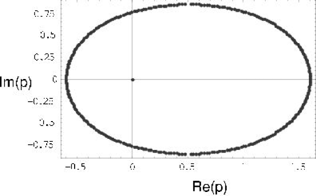
Figure 11: Location of the roots of Rel2(n=150)(p)=0superscriptsubscriptRel2𝑛150𝑝0{\rm Rel}_{2}^{(n=150)}(p)=0 for the fan, with ρ=1𝜌1\rho=1.

For ρ=1𝜌1\rho=1, we see on Figure 11 that the limiting curve is now essentially a closed one, even though the zeros appear to belong to two different sets which slowly join as n𝑛n increases. The presence of n𝑛n in a prefactor as in eqs. (59) and (60) does not affect the general definition of the limiting curves [8]. The limiting curve is very easy to obtain, since we have only two eigenvalues, 1 and p(1p)𝑝1𝑝p\,(1-p). For them to have the same modulus implies p(1p)=eiθ𝑝1𝑝superscript𝑒𝑖𝜃p\,(1-p)=-e^{i\,\theta}, so that we get p=12(1±1+4eiθ)𝑝12plus-or-minus114superscript𝑒𝑖𝜃p=\frac{1}{2}\,\left(1\pm\sqrt{1+4\,e^{i\,\theta}}\right).

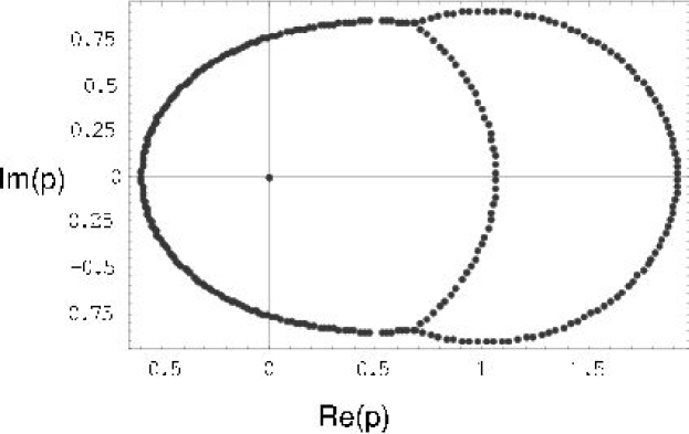
When ρ𝜌\rho is strictly less than 1, the whole structure is altered, as witnessed by Figure 12 for ρ=0.9999𝜌0.9999\rho=0.9999. Portions of circles centered at the origin and at the point (1,0)10(1,0) are added. The reason for such additional structures comes from the existence of a new eigenvalue pρ𝑝𝜌p\,\rho. They persist down to ρ=12𝜌12\rho=\frac{1}{2}. For ρ<12𝜌12\rho<\frac{1}{2}, the only eigenvalues that matter are actually 1 and p(1p)ρ𝑝1𝑝𝜌p\,(1-p)\,\rho, so that the structure looks again very much like Fig. 11.

Refer to caption
Figure 12: Location of the roots of Rel2(n=150)(p)=0superscriptsubscriptRel2𝑛150𝑝0{\rm Rel}_{2}^{(n=150)}(p)=0 for the fan, with ρ=0.9999𝜌0.9999\rho=0.9999.
Table 3: Analytical expressions of the limiting aggregation curves for the location of p𝑝p such that Rel2(fan),n(p,ρ)=0superscriptsubscriptRel2fan𝑛𝑝𝜌0{\rm Rel}_{2}^{{\rm(fan)},n\rightarrow\infty}(p,\rho)=0, as a function of ρ𝜌\rho, the node reliability.
node reliability parametrization validity range
ρ=1𝜌1\rho=1 p=12(1±1+4eiθ)𝑝12plus-or-minus114superscript𝑒𝑖𝜃p=\frac{1}{2}\,\left(1\pm\sqrt{1+4\,e^{i\,\theta}}\right) 1cosθ11𝜃1-1\leq\cos\theta\leq 1
12<ρ<112𝜌1\frac{1}{2}<\rho<1 p=12(11+4ρeiθ)p=12(1+1+4ρeiθ)p=1ρeiθp=1+eiθ𝑝12114𝜌superscript𝑒𝑖𝜃𝑝12114𝜌superscript𝑒𝑖𝜃𝑝1𝜌superscript𝑒𝑖𝜃𝑝1superscript𝑒𝑖𝜃\displaystyle\begin{array}[]{l}p=\frac{1}{2}\,\left(1-\sqrt{1+\frac{4}{\rho}\,e^{i\,\theta}}\right)\\[5.69054pt] p=\frac{1}{2}\,\left(1+\sqrt{1+\frac{4}{\rho}\,e^{i\,\theta}}\right)\\[5.69054pt] p=\frac{1}{\rho}\,e^{i\,\theta}\\[5.69054pt] p=1+e^{i\,\theta}\end{array} 1cosθ11cosθ12ρ(1ρ23)cosθ12ρcosθ12ρ211𝜃11𝜃12𝜌1superscript𝜌23𝜃12𝜌𝜃12superscript𝜌21\displaystyle\begin{array}[]{l}-1\leq\cos\theta\leq 1\\[5.69054pt] -1\leq\cos\theta\leq\frac{1}{2\,\rho}\,\left(\frac{1}{\rho^{2}}-3\right)\\[5.69054pt] \cos\theta\geq\frac{1}{2\,\rho}\\[5.69054pt] \cos\theta\geq\frac{1}{2\,\rho^{2}}-1\end{array}
0<ρ120𝜌120<\rho\leq\frac{1}{2} p=12(1±1+4ρeiθ)𝑝12plus-or-minus114𝜌superscript𝑒𝑖𝜃p=\frac{1}{2}\,\left(1\pm\sqrt{1+\frac{4}{\rho}\,e^{i\,\theta}}\right) 1cosθ11𝜃1-1\leq\cos\theta\leq 1

Their derivation being straightforward, we simply give the analytical expressions of the limiting curves in Table 3. When ρ0𝜌0\rho\rightarrow 0, the structure expands with a scaling factor of ρ1/2superscript𝜌12\rho^{-1/2}, in contrast with the ρ1/3superscript𝜌13\rho^{-1/3} obtained for the Brecht-Colbourn ladder.

6 All-terminal reliability

As mentioned in the introduction, the all-terminal reliability RelAsubscriptRel𝐴{\rm Rel}_{A} is another useful measure of the network availability, giving the probability that all nodes are connected. In this case however, the node reliabilities are a mere overall factor, so that they may be considered equal to 1 for all practical purposes [26]. Chang and Shrock [19] gave the explicit expressions of RelAsubscriptRel𝐴{\rm Rel}_{A} for various recursive families of graphs, among which the Brecht-Colbourn ladder, with the same reliability p𝑝p for all edges. The all-terminal reliability of the generalized fan has been calculated by Neufeld and Colbourn [49]. The results are of course identical, because at each step, two edges are added, while the common original graph is the triangle (the complete graph K3subscript𝐾3K_{3}). For the sake of completeness, we slightly generalize their result for edges with distinct reliabilities. Here again, the final, analytical expression can be written in a concise form using transfer matrices. In the context of graph theory, this can be viewed as the factorization of a particular value of the multi-variate Tutte polynomial, considered by Wu [74] and Sokal [64].

Refer to caption
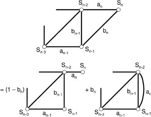
Figure 13: Deletion-contraction simplification for the all-terminal reliability of the Brecht-Colbourn ladder.

We expect the all-terminal reliability n=RelA(S0Sn){\mathcal{R}}_{n}={\rm Rel}_{A}(S_{0}\leftrightarrow S_{n}) for the Brecht-Colbourn ladder to exhibit the same behavior as the two-terminal reliability, with a transfer matrix depending on ansubscript𝑎𝑛a_{n} and bnsubscript𝑏𝑛b_{n}, and a generating function that is a rational fraction of p𝑝p (the common reliability of links) and z𝑧z. As mentioned above, this calculation should be somewhat easier because all nodes can be considered perfect without loss of generality [26]. We can then use the usual pivotal decomposition to establish a relationship between nsubscript𝑛{\mathcal{R}}_{n} and n1subscript𝑛1{\mathcal{R}}_{n-1}, as represented in Fig. 13. We find

n=(1bn)ann1+bnn1(bn1bn1//an){\mathcal{R}}_{n}=(1-b_{n})\,a_{n}\,{\mathcal{R}}_{n-1}+b_{n}\,{\mathcal{R}}_{n-1}(b_{n-1}\rightarrow b_{n-1}\,//\,a_{n}) (76)

Using the ansatz n=αn(an+bn)+γnanbnsubscript𝑛subscript𝛼𝑛subscript𝑎𝑛subscript𝑏𝑛subscript𝛾𝑛subscript𝑎𝑛subscript𝑏𝑛{\mathcal{R}}_{n}=\alpha_{n}\,(a_{n}+b_{n})+\gamma_{n}\,a_{n}\,b_{n}, we get

(αnγn)=(an1+bn1an1bn11an12bn1an1(12bn1))(αn1γn1)subscript𝛼𝑛subscript𝛾𝑛subscript𝑎𝑛1subscript𝑏𝑛1subscript𝑎𝑛1subscript𝑏𝑛1missing-subexpressionmissing-subexpression1subscript𝑎𝑛12subscript𝑏𝑛1subscript𝑎𝑛112subscript𝑏𝑛1subscript𝛼𝑛1subscript𝛾𝑛1\left(\begin{array}[]{l}\alpha_{n}\\ \gamma_{n}\end{array}\right)=\left(\begin{array}[]{l|l}a_{n-1}+b_{n-1}&a_{n-1}\,b_{n-1}\\ \hline\cr 1-a_{n-1}-2\,b_{n-1}&a_{n-1}\,\big{(}1-2\,b_{n-1}\big{)}\end{array}\right)\;\left(\begin{array}[]{l}\alpha_{n-1}\\ \gamma_{n-1}\end{array}\right) (77)

with a1=γ1=0subscript𝑎1subscript𝛾10a_{1}=\gamma_{1}=0 and α1=1subscript𝛼11\alpha_{1}=1. Calling M~n1subscript~𝑀𝑛1\widetilde{M}_{n-1} the transfer matrix of eq. (77), we obtain

n=(1,0)M~nM~n1M~1(10)subscript𝑛10subscript~𝑀𝑛subscript~𝑀𝑛1subscript~𝑀110{\mathcal{R}}_{n}=(1,0)\;\cdot\;\widetilde{M}_{n}\;\cdot\;\widetilde{M}_{n-1}\;\cdots\;\widetilde{M}_{1}\;\cdot\;\left(\begin{array}[]{l}1\\ 0\end{array}\right) (78)

When all reliabilities are equal to p𝑝p, the transfer matrix is simply

M~=(2pp213pp(12p))~superscript𝑀2𝑝superscript𝑝2missing-subexpressionmissing-subexpression13𝑝𝑝12𝑝\widetilde{M^{\prime}}=\left(\begin{array}[]{l|l}2\,p&p^{2}\\ \hline\cr 1-3\,p&p\,(1-2\,p)\end{array}\right) (79)

The eigenvalues of M~~superscript𝑀\widetilde{M^{\prime}} are ζ±=p2(32p±58p+4p2)subscript𝜁plus-or-minus𝑝2plus-or-minus32𝑝58𝑝4superscript𝑝2\displaystyle\zeta_{\pm}=\frac{p}{2}\;\left(3-2\,p\pm\sqrt{5-8\,p+4\,p^{2}}\right), so that the generating function is

GR(z)=pz21p(32p)z+p2(1p)z2subscript𝐺𝑅𝑧𝑝superscript𝑧21𝑝32𝑝𝑧superscript𝑝21𝑝superscript𝑧2G_{R}(z)=\frac{p\,z^{2}}{1-p\,(3-2\,p)\,z+p^{2}\,(1-p)\,z^{2}} (80)

and

n=158p+4p2(ζ+n1ζn1)n2subscript𝑛158𝑝4superscript𝑝2superscriptsubscript𝜁𝑛1superscriptsubscript𝜁𝑛1𝑛2{\mathcal{R}}_{n}=\frac{1}{\sqrt{5-8\,p+4\,p^{2}}}\;\left(\zeta_{+}^{n-1}-\zeta_{-}^{n-1}\right)\hskip 28.45274ptn\geq 2 (81)

The last results were obtained in [19], while the same expression can be found in the paper by Neufeld and Colbourn [49].

7 Conclusion and Perspectives

We have given the exact solution of the two- and all-terminal reliabilities for the Brecht-Colbourn ladder and the generalized fan for arbitrary size and individual element reliability. While simple, these graphs correspond nonetheless to realistic network architectures, especially in telecommunication networks for IP transport. Node and edge failures are put on an equal footing, and the simple formulae relying on transfer matrices may be directly implemented. We have also given the analytical solution of the two- and all-terminal reliabilities, when reliabilities are p𝑝p and ρ𝜌\rho for edges and nodes, along with their rational generating functions. The locations of the zeros of the two-terminal reliability polynomials differ for the two families of graphs considered in this paper, even though their all-terminal reliability is identical. They possess structures in the Re(p)<0Re𝑝0{\rm Re}(p)<0 region, and exhibit transitions for particular values of ρ𝜌\rho.

Even though the delta-star transformation has also been successfully applied to the case of simple ladders [66], it may not be so easy to use in more complicated networks. However, it seems quite clear that a similar decomposition through transfer matrices of two-terminal reliabilities should occur for ladders of greater width too. In order to make such calculations useful for applications, imperfect nodes as well as imperfect edges must be considered. All is needed is a recursion relation between successive graphs, when one “elementary brick” is added. This implies a new expression for the deletion-contraction theorem, in which the linearity with respect to all individual edge or node reliabilities must be preserved, whereas — to our knowledge — edge reliabilities are often renormalized to account for the unreliability of the nodes they connect [3, 70, 71]. This new expression will be given elsewhere, along with an application to other recursive families of graphs such as the K4subscript𝐾4K_{4} ladder and the K3subscript𝐾3K_{3} cylinder [67].

What should we expect ? Basically, the same kind of behavior as detailed in the present work, with a factorization of the reliability in terms of transfer matrices, the dimension of which substantially increase to reflect the interplay of different edges/nodes in the overall reliability, and the underlying algebraic structure of the graph (one cannot escape the intrinsic complexity of the problem…).

There are obviously many directions in which this work may be further extended, for instance in the estimates of bounds. The first one is to use the present results, or their future extensions [67, 69], as possible upper or lower bounds to more complex graphs. If a graph under consideration looks like — or made as such — a special instance of a recursive family of graphs, we expect the generating function to be a rational fraction again. The dimension of the corresponding transfer matrix may be probed by trying to find recursion relations between successive reliability polynomials. Of course, if the dimension of the corresponding transfer matrix is large — which is most likely to happen — the degree of the numerator and denominator of the fraction may be too large for a complete solution to be obtained easily. Even so, the knowledge that the true generating function is rational may be an indication that an approximate generating function might still be quite useful, because Padé approximants[4, 50] are known for their devilish knack of getting very close to the exact function. This will be addressed elsewhere [69]. Our calculations may also provide some information on some combinatorial issues, such as the enumeration of self-avoiding walks on lattices of restricted width.

Other quantities of interest may be deduced from the general expression of the network reliability, among them the sensitivity of a equipment [66], the influence of scheduled maintenance on the overall network availability, and the failure frequency [37, 62], which can all be deduced from various partial derivatives of the two- and all-terminal reliabilities [68]. Since the reliability of each equipment appears in only one transfer matrix, the computation of all these network parameters is straightforward. One should also be aware that the reliability of each equipment is not known with absolute accuracy. The consequence of this uncertainty on the overall reliability has been addressed by Coit and collaborators in the case of series-parallel reducible networks [24, 25]. Our transfer matrix factorization makes this topic another instance of a product of random matrices, definitely a vast field in mathematical physics [29].

Finally, the exact results found for classes of arbitrarily large networks may prove useful for testing different algorithms (Monte Carlo, genetic, OBDD, etc) in numerically exacting configurations, where edge and node unreliabilities must both be taken into account.

Acknowledgments

I am indebted to Élisabeth Didelet for giving me the opportunity to study reliability issues in depth, and to Joël Le Meur, François Gallant, Veluppillai Chandrakumar, Adam Ouorou, and Éric Gourdin for encouragement and support. Useful information from Prof. J. Graver is gratefully acknowledged. I would also like to thank Annie Druault-Vicard, Christine Leroy, Hervé Coutelle, and Gilles Petitdemange for very useful discussions.

Appendix A Polynomials used in the determination of critical points for the zeros of Rel2(p)subscriptRel2𝑝{\rm Rel}_{2}(p) (Brecht-Colbourn ladder)

A.1 𝒫1(p,ρ)subscript𝒫1𝑝𝜌{\mathcal{P}}_{1}(p,\rho)

𝒫1(p,ρ)subscript𝒫1𝑝𝜌\displaystyle{\mathcal{P}}_{1}(p,\rho) =\displaystyle= ρp(1+9ρ+3ρ2)+p2ρ(41+37ρ11ρ2)𝜌𝑝19𝜌3superscript𝜌2superscript𝑝2𝜌4137𝜌11superscript𝜌2\displaystyle\rho-p\,\left(1+9\,\rho+3\,{\rho}^{2}\right)+p^{2}\,\rho\,\left(41+37\,\rho-11\,{\rho}^{2}\right) (82)
+p3ρ(39195ρ+99ρ24ρ3)superscript𝑝3𝜌39195𝜌99superscript𝜌24superscript𝜌3\displaystyle+p^{3}\,\rho\,\left(-39-195\,\rho+99\,{\rho}^{2}-4\,{\rho}^{3}\right)
+p4ρ(16+147ρ411ρ2+43ρ3+11ρ4)superscript𝑝4𝜌16147𝜌411superscript𝜌243superscript𝜌311superscript𝜌4\displaystyle+p^{4}\,\rho\,\left(16+147\,\rho-411\,{\rho}^{2}+43\,{\rho}^{3}+11\,{\rho}^{4}\right)
p5ρ2(542300ρ+123ρ2+67ρ3+7ρ4)superscript𝑝5superscript𝜌2542300𝜌123superscript𝜌267superscript𝜌37superscript𝜌4\displaystyle-p^{5}\,\rho^{2}\,\left(-54-2300\,\rho+123\,{\rho}^{2}+67\,{\rho}^{3}+7\,{\rho}^{4}\right)
p6ρ2(126+4700ρ+1865ρ2+559ρ359ρ4+13ρ5)superscript𝑝6superscript𝜌21264700𝜌1865superscript𝜌2559superscript𝜌359superscript𝜌413superscript𝜌5\displaystyle-p^{6}\,\rho^{2}\,\left(126+4700\,\rho+1865\,{\rho}^{2}+559\,{\rho}^{3}-59\,{\rho}^{4}+13\,{\rho}^{5}\right)
+p7ρ2(41+4859ρ+2324ρ2+6400ρ3+1135ρ4+189ρ5+14ρ6)superscript𝑝7superscript𝜌2414859𝜌2324superscript𝜌26400superscript𝜌31135superscript𝜌4189superscript𝜌514superscript𝜌6\displaystyle+p^{7}\,\rho^{2}\,\left(41+4859\,\rho+2324\,{\rho}^{2}+6400\,{\rho}^{3}+1135\,{\rho}^{4}+189\,{\rho}^{5}+14\,{\rho}^{6}\right)
+p8ρ3(2701+4149ρ11762ρ28744ρ32515ρ4311ρ5+4ρ6)superscript𝑝8superscript𝜌327014149𝜌11762superscript𝜌28744superscript𝜌32515superscript𝜌4311superscript𝜌54superscript𝜌6\displaystyle+p^{8}\,{\rho}^{3}\,\left(-2701+4149\,\rho-11762\,{\rho}^{2}-8744\,{\rho}^{3}-2515\,{\rho}^{4}-311\,{\rho}^{5}+4\,{\rho}^{6}\right)
p9ρ3(781+12546ρ6054ρ214564ρ311548ρ43012ρ5124ρ6+8ρ7)superscript𝑝9superscript𝜌378112546𝜌6054superscript𝜌214564superscript𝜌311548superscript𝜌43012superscript𝜌5124superscript𝜌68superscript𝜌7\displaystyle-p^{9}\,{\rho}^{3}\,\left(-781+12546\,\rho-6054\,{\rho}^{2}-14564\,{\rho}^{3}-11548\,{\rho}^{4}-3012\,{\rho}^{5}-124\,{\rho}^{6}+8\,{\rho}^{7}\right)
p10ρ3(9613197ρ3996ρ2+4727ρ3+17901ρ4+11943ρ5+1464ρ6+4ρ7)superscript𝑝10superscript𝜌39613197𝜌3996superscript𝜌24727superscript𝜌317901superscript𝜌411943superscript𝜌51464superscript𝜌64superscript𝜌7\displaystyle-p^{10}\,{\rho}^{3}\,\left(96-13197\,\rho-3996\,{\rho}^{2}+4727\,{\rho}^{3}+17901\,{\rho}^{4}+11943\,{\rho}^{5}+1464\,{\rho}^{6}+4\,{\rho}^{7}\right)
+p11ρ4(71853814ρ10626ρ2+5695ρ3+21337ρ4+5871ρ5+304ρ6)superscript𝑝11superscript𝜌471853814𝜌10626superscript𝜌25695superscript𝜌321337superscript𝜌45871superscript𝜌5304superscript𝜌6\displaystyle+p^{11}\,{\rho}^{4}\,\left(-7185-3814\,\rho-10626\,{\rho}^{2}+5695\,{\rho}^{3}+21337\,{\rho}^{4}+5871\,{\rho}^{5}+304\,{\rho}^{6}\right)
p12ρ4(2040+3598ρ10478ρ217573ρ3+19235ρ4+11669ρ5+1219ρ6)superscript𝑝12superscript𝜌420403598𝜌10478superscript𝜌217573superscript𝜌319235superscript𝜌411669superscript𝜌51219superscript𝜌6\displaystyle-p^{12}\,{\rho}^{4}\,\left(-2040+3598\,\rho-10478\,{\rho}^{2}-17573\,{\rho}^{3}+19235\,{\rho}^{4}+11669\,{\rho}^{5}+1219\,{\rho}^{6}\right)
+p13ρ4(240+6353ρ+3091ρ230176ρ3+6625ρ4+14726ρ5+2128ρ6)superscript𝑝13superscript𝜌42406353𝜌3091superscript𝜌230176superscript𝜌36625superscript𝜌414726superscript𝜌52128superscript𝜌6\displaystyle+p^{13}\,{\rho}^{4}\,\left(-240+6353\,\rho+3091\,{\rho}^{2}-30176\,{\rho}^{3}+6625\,{\rho}^{4}+14726\,{\rho}^{5}+2128\,{\rho}^{6}\right)
p14ρ5(3613+12361ρ25852ρ25221ρ3+14188ρ4+2147ρ5)superscript𝑝14superscript𝜌5361312361𝜌25852superscript𝜌25221superscript𝜌314188superscript𝜌42147superscript𝜌5\displaystyle-p^{14}\,{\rho}^{5}\,\left(3613+12361\,\rho-25852\,{\rho}^{2}-5221\,{\rho}^{3}+14188\,{\rho}^{4}+2147\,{\rho}^{5}\right)
+p15ρ5(947+11148ρ14935ρ28341ρ3+9720ρ4+2095ρ5)superscript𝑝15superscript𝜌594711148𝜌14935superscript𝜌28341superscript𝜌39720superscript𝜌42095superscript𝜌5\displaystyle+p^{15}\,{\rho}^{5}\,\left(947+11148\,\rho-14935\,{\rho}^{2}-8341\,{\rho}^{3}+9720\,{\rho}^{4}+2095\,{\rho}^{5}\right)
p16ρ5(96+5829ρ7507ρ21909ρ3+690ρ4+3066ρ5)superscript𝑝16superscript𝜌5965829𝜌7507superscript𝜌21909superscript𝜌3690superscript𝜌43066superscript𝜌5\displaystyle-p^{16}\,{\rho}^{5}\,\left(96+5829\,\rho-7507\,{\rho}^{2}-1909\,{\rho}^{3}+690\,{\rho}^{4}+3066\,{\rho}^{5}\right)
+2p17ρ6(9932513ρ+3568ρ24056ρ3+2046ρ4)2superscript𝑝17superscript𝜌69932513𝜌3568superscript𝜌24056superscript𝜌32046superscript𝜌4\displaystyle+2\,p^{17}\,{\rho}^{6}\,\left(993-2513\,\rho+3568\,{\rho}^{2}-4056\,{\rho}^{3}+2046\,{\rho}^{4}\right)
p18ρ6(4183991ρ+10333ρ210532ρ3+3785ρ4)superscript𝑝18superscript𝜌64183991𝜌10333superscript𝜌210532superscript𝜌33785superscript𝜌4\displaystyle-p^{18}\,{\rho}^{6}\,\left(418-3991\,\rho+10333\,{\rho}^{2}-10532\,{\rho}^{3}+3785\,{\rho}^{4}\right)
+p19ρ6(412397ρ+7184ρ27257ρ3+2430ρ4)superscript𝑝19superscript𝜌6412397𝜌7184superscript𝜌27257superscript𝜌32430superscript𝜌4\displaystyle+p^{19}\,{\rho}^{6}\,\left(41-2397\,\rho+7184\,{\rho}^{2}-7257\,{\rho}^{3}+2430\,{\rho}^{4}\right)
+3p20(1ρ)ρ7(299684ρ+367ρ2)3superscript𝑝201𝜌superscript𝜌7299684𝜌367superscript𝜌2\displaystyle+3\,p^{20}\,\left(1-\rho\right)\,{\rho}^{7}\,\left(299-684\,\rho+367\,{\rho}^{2}\right)
p21(1ρ)ρ7(185519ρ+322ρ2)superscript𝑝211𝜌superscript𝜌7185519𝜌322superscript𝜌2\displaystyle-p^{21}\,\left(1-\rho\right)\,{\rho}^{7}\,\left(185-519\,\rho+322\,{\rho}^{2}\right)
+p22(1ρ)ρ7(12ρ)(1615ρ)superscript𝑝221𝜌superscript𝜌712𝜌1615𝜌\displaystyle+p^{22}\,\left(1-\rho\right)\,{\rho}^{7}\,\left(1-2\,\rho\right)\,\left(16-15\,\rho\right)
19p23(1ρ)2ρ8+8p24(1ρ)2ρ8p25(1ρ)2ρ819superscript𝑝23superscript1𝜌2superscript𝜌88superscript𝑝24superscript1𝜌2superscript𝜌8superscript𝑝25superscript1𝜌2superscript𝜌8\displaystyle-19\,p^{23}\,{\left(1-\rho\right)}^{2}\,{\rho}^{8}+8\,p^{24}\,{\left(1-\rho\right)}^{2}\,{\rho}^{8}-p^{25}\,{\left(1-\rho\right)}^{2}\,{\rho}^{8}

A.2 𝒫2(p,ρ)subscript𝒫2𝑝𝜌{\mathcal{P}}_{2}(p,\rho)

𝒫2(p,ρ)subscript𝒫2𝑝𝜌\displaystyle{\mathcal{P}}_{2}(p,\rho) =\displaystyle= (83)
9+2p(93+37ρ)+p2(13751139ρ+235ρ2)92𝑝9337𝜌superscript𝑝213751139𝜌235superscript𝜌2\displaystyle\hskip-56.9055pt9+2\,p\,\left(-93+37\,\rho\right)+p^{2}\,\left(1375-1139\,\rho+235\,{\rho}^{2}\right)
+p3(4548+6619ρ2306ρ2+380ρ3)superscript𝑝345486619𝜌2306superscript𝜌2380superscript𝜌3\displaystyle\hskip-56.9055pt+p^{3}\,\left(-4548+6619\,\rho-2306\,{\rho}^{2}+380\,{\rho}^{3}\right)
+p4(755122762ρ+7011ρ22415ρ3+335ρ4)superscript𝑝4755122762𝜌7011superscript𝜌22415superscript𝜌3335superscript𝜌4\displaystyle\hskip-56.9055pt+p^{4}\,\left(7551-22762\,\rho+7011\,{\rho}^{2}-2415\,{\rho}^{3}+335\,{\rho}^{4}\right)
+p5(6210+53479ρ+2160ρ2+7102ρ31462ρ4+154ρ5)superscript𝑝5621053479𝜌2160superscript𝜌27102superscript𝜌31462superscript𝜌4154superscript𝜌5\displaystyle\hskip-56.9055pt+p^{5}\,\left(-6210+53479\,\rho+2160\,{\rho}^{2}+7102\,{\rho}^{3}-1462\,{\rho}^{4}+154\,{\rho}^{5}\right)
+p6(202585209ρ79460ρ218121ρ311141ρ4+223ρ5+29ρ6)superscript𝑝6202585209𝜌79460superscript𝜌218121superscript𝜌311141superscript𝜌4223superscript𝜌529superscript𝜌6\displaystyle\hskip-56.9055pt+p^{6}\,\left(2025-85209\,\rho-79460\,{\rho}^{2}-18121\,{\rho}^{3}-11141\,{\rho}^{4}+223\,{\rho}^{5}+29\,{\rho}^{6}\right)
+p7ρ(84879+277027ρ+106511ρ2+202610ρ336581ρ4+1170ρ5)superscript𝑝7𝜌84879277027𝜌106511superscript𝜌2202610superscript𝜌336581superscript𝜌41170superscript𝜌5\displaystyle\hskip-56.9055pt+p^{7}\,\rho\,\left(84879+277027\,\rho+106511\,{\rho}^{2}+202610\,{\rho}^{3}-36581\,{\rho}^{4}+1170\,{\rho}^{5}\right)
+p8ρ(46170521894ρ587852ρ21536749ρ3+263741ρ439391ρ5+547ρ6)superscript𝑝8𝜌46170521894𝜌587852superscript𝜌21536749superscript𝜌3263741superscript𝜌439391superscript𝜌5547superscript𝜌6\displaystyle\hskip-56.9055pt+p^{8}\,\rho\,\left(-46170-521894\,\rho-587852\,{\rho}^{2}-1536749\,{\rho}^{3}+263741\,{\rho}^{4}-39391\,{\rho}^{5}+547\,{\rho}^{6}\right)
p9ρ(10125611502ρ1935829ρ27279427ρ3+440373ρ4\displaystyle\hskip-56.9055pt-p^{9}\,\rho\,\left(-10125-611502\,\rho-1935829\,{\rho}^{2}-7279427\,{\rho}^{3}+440373\,{\rho}^{4}\right.
331984ρ5+16780ρ6)\displaystyle\hskip-14.22636pt\left.-331984\,{\rho}^{5}+16780\,{\rho}^{6}\right)
+p10ρ2(4557963964687ρ23412205ρ23663927ρ31452867ρ4\displaystyle\hskip-56.9055pt+p^{10}\,{\rho}^{2}\,\left(-455796-3964687\,\rho-23412205\,{\rho}^{2}-3663927\,{\rho}^{3}-1452867\,{\rho}^{4}\right.
+375501ρ5+2506ρ6)\displaystyle\hskip-14.22636pt\left.+375501\,{\rho}^{5}+2506\,{\rho}^{6}\right)
+p11ρ2(204255+5324974ρ+53128592ρ2+28420289ρ3+5054943ρ4\displaystyle\hskip-56.9055pt+p^{11}\,{\rho}^{2}\,\left(204255+5324974\,\rho+53128592\,{\rho}^{2}+28420289\,{\rho}^{3}+5054943\,{\rho}^{4}\right.
4185113ρ5+12850ρ6)\displaystyle\hskip-14.22636pt\left.-4185113\,{\rho}^{5}+12850\,{\rho}^{6}\right)
+p12ρ2(425254776213ρ87000246ρ2104194583ρ3\displaystyle\hskip-56.9055pt+p^{12}\,{\rho}^{2}\,\left(-42525-4776213\,\rho-87000246\,{\rho}^{2}-104194583\,{\rho}^{3}\right.
21210055ρ4+27622695ρ5279589ρ6+23497ρ7)\displaystyle\hskip-14.22636pt\left.-21210055\,{\rho}^{4}+27622695\,{\rho}^{5}-279589\,{\rho}^{6}+23497\,{\rho}^{7}\right)
+p13ρ3(2798298+103839446ρ+248730949ρ2+91081790ρ3\displaystyle\hskip-56.9055pt+p^{13}\,{\rho}^{3}\,\left(2798298+103839446\,\rho+248730949\,{\rho}^{2}+91081790\,{\rho}^{3}\right.
119321953ρ4214483ρ5+2402ρ6)\displaystyle\hskip-14.22636pt\left.-119321953\,{\rho}^{4}-214483\,{\rho}^{5}+2402\,{\rho}^{6}\right)
+p14ρ3(98766090012828ρ421343630ρ2300983008ρ3\displaystyle\hskip-56.9055pt+p^{14}\,{\rho}^{3}\,\left(-987660-90012828\,\rho-421343630\,{\rho}^{2}-300983008\,{\rho}^{3}\right.
+354546288ρ4+19055623ρ52902607ρ6+156356ρ7)\displaystyle\hskip-14.22636pt\left.+354546288\,{\rho}^{4}+19055623\,{\rho}^{5}-2902607\,{\rho}^{6}+156356\,{\rho}^{7}\right)
p15ρ3(16402555522953ρ523811627ρ2718737692ρ3\displaystyle\hskip-56.9055pt-p^{15}\,{\rho}^{3}\,\left(-164025-55522953\,\rho-523811627\,{\rho}^{2}-718737692\,{\rho}^{3}\right.
+737559653ρ4+137144016ρ524588235ρ6+1508228ρ7)\displaystyle\hskip-14.22636pt\left.+737559653\,{\rho}^{4}+137144016\,{\rho}^{5}-24588235\,{\rho}^{6}+1508228\,{\rho}^{7}\right)
+p16ρ4(23264478483102731ρ1256125498ρ2+1050744677ρ3\displaystyle\hskip-56.9055pt+p^{16}\,{\rho}^{4}\,\left(-23264478-483102731\,\rho-1256125498\,{\rho}^{2}+1050744677\,{\rho}^{3}\right.
+534128347ρ499647028ρ5+3934654ρ6+455372ρ7)\displaystyle\hskip-14.22636pt\left.+534128347\,{\rho}^{4}-99647028\,{\rho}^{5}+3934654\,{\rho}^{6}+455372\,{\rho}^{7}\right)
p17ρ4(5993055328891636ρ1637004249ρ2+897069980ρ3\displaystyle\hskip-56.9055pt-p^{17}\,{\rho}^{4}\,\left(-5993055-328891636\,\rho-1637004249\,{\rho}^{2}+897069980\,{\rho}^{3}\right.
+1365985483ρ4226306853ρ513885678ρ6+5675792ρ7)\displaystyle\hskip-14.22636pt\left.+1365985483\,{\rho}^{4}-226306853\,{\rho}^{5}-13885678\,{\rho}^{6}+5675792\,{\rho}^{7}\right)
+p18ρ4(729000161715291ρ1608420692ρ2+82688597ρ3+2449767599ρ4\displaystyle\hskip-56.9055pt+p^{18}\,{\rho}^{4}\,\left(-729000-161715291\,\rho-1608420692\,{\rho}^{2}+82688597\,{\rho}^{3}+2449767599\,{\rho}^{4}\right.
232309325ρ5139531559ρ6+32366472ρ7+274104ρ8)\displaystyle\hskip-14.22636pt\left.-232309325\,{\rho}^{5}-139531559\,{\rho}^{6}+32366472\,{\rho}^{7}+274104\,{\rho}^{8}\right)
p19ρ5(547793281192868328ρ1036350248ρ2+3126514952ρ3\displaystyle\hskip-56.9055pt-p^{19}\,{\rho}^{5}\,\left(-54779328-1192868328\,\rho-1036350248\,{\rho}^{2}+3126514952\,{\rho}^{3}\right.
+252124085ρ4530576442ρ5+110376920ρ6+3523400ρ7)\displaystyle\hskip-14.22636pt\left.+252124085\,{\rho}^{4}-530576442\,{\rho}^{5}+110376920\,{\rho}^{6}+3523400\,{\rho}^{7}\right)
+p20ρ5(11563290661113157ρ1778966082ρ2+2728489572ρ3\displaystyle\hskip-56.9055pt+p^{20}\,{\rho}^{5}\,\left(-11563290-661113157\,\rho-1778966082\,{\rho}^{2}+2728489572\,{\rho}^{3}\right.
+1464568704ρ41261931324ρ5+243789711ρ6+21533484ρ7)\displaystyle\hskip-14.22636pt\left.+1464568704\,{\rho}^{4}-1261931324\,{\rho}^{5}+243789711\,{\rho}^{6}+21533484\,{\rho}^{7}\right)
p21ρ5(1166400267060831ρ1769360761ρ2+1310882671ρ3\displaystyle\hskip-56.9055pt-p^{21}\,{\rho}^{5}\,\left(-1166400-267060831\,\rho-1769360761\,{\rho}^{2}+1310882671\,{\rho}^{3}\right.
+3038379428ρ42084661610ρ5+338855326ρ6+82890944ρ7)\displaystyle\hskip-14.22636pt\left.+3038379428\,{\rho}^{4}-2084661610\,{\rho}^{5}+338855326\,{\rho}^{6}+82890944\,{\rho}^{7}\right)
+p22ρ6(748248121221905422ρ276377214ρ2+4066473373ρ3\displaystyle\hskip-56.9055pt+p^{22}\,{\rho}^{6}\,\left(-74824812-1221905422\,\rho-276377214\,{\rho}^{2}+4066473373\,{\rho}^{3}\right.
2443698651ρ4+202709670ρ5+224730742ρ6)\displaystyle\hskip-14.22636pt\left.-2443698651\,{\rho}^{4}+202709670\,{\rho}^{5}+224730742\,{\rho}^{6}\right)
p23ρ6(13126860609332834ρ1166508009ρ2+3871377708ρ3\displaystyle\hskip-56.9055pt-p^{23}\,{\rho}^{6}\,\left(-13126860-609332834\,\rho-1166508009\,{\rho}^{2}+3871377708\,{\rho}^{3}\right.
1932786432ρ4295096153ρ5+454945390ρ6)\displaystyle\hskip-14.22636pt\left.-1932786432\,{\rho}^{4}-295096153\,{\rho}^{5}+454945390\,{\rho}^{6}\right)
+p24ρ6(1103625218082828ρ1184923715ρ2+2650067734ρ3\displaystyle\hskip-56.9055pt+p^{24}\,{\rho}^{6}\,\left(-1103625-218082828\,\rho-1184923715\,{\rho}^{2}+2650067734\,{\rho}^{3}\right.
752045795ρ41022894704ρ5+711726527ρ6)\displaystyle\hskip-14.22636pt\left.-752045795\,{\rho}^{4}-1022894704\,{\rho}^{5}+711726527\,{\rho}^{6}\right)
p25ρ7(53743284754572613ρ+1226487190ρ2+416790514ρ3\displaystyle\hskip-56.9055pt-p^{25}\,{\rho}^{7}\,\left(-53743284-754572613\,\rho+1226487190\,{\rho}^{2}+416790514\,{\rho}^{3}\right.
1614449937ρ4+878716880ρ5)\displaystyle\hskip-14.22636pt\left.-1614449937\,{\rho}^{4}+878716880\,{\rho}^{5}\right)
+p26ρ7(8258625336506619ρ+274671788ρ2+1010093115ρ3\displaystyle\hskip-56.9055pt+p^{26}\,{\rho}^{7}\,\left(-8258625-336506619\,\rho+274671788\,{\rho}^{2}+1010093115\,{\rho}^{3}\right.
1758220080ρ4+866894232ρ5)\displaystyle\hskip-14.22636pt\left.-1758220080\,{\rho}^{4}+866894232\,{\rho}^{5}\right)
p27ρ7(605475106456428ρ91817943ρ2+978393477ρ3\displaystyle\hskip-56.9055pt-p^{27}\,{\rho}^{7}\,\left(-605475-106456428\,\rho-91817943\,{\rho}^{2}+978393477\,{\rho}^{3}\right.
1446294368ρ4+687560517ρ5)\displaystyle\hskip-14.22636pt\left.-1446294368\,{\rho}^{4}+687560517\,{\rho}^{5}\right)
+p28ρ8(23082921120749456ρ+640575958ρ2928058750ρ3+438708098ρ4)superscript𝑝28superscript𝜌823082921120749456𝜌640575958superscript𝜌2928058750superscript𝜌3438708098superscript𝜌4\displaystyle\hskip-56.9055pt+p^{28}\,{\rho}^{8}\,\left(-23082921-120749456\,\rho+640575958\,{\rho}^{2}-928058750\,{\rho}^{3}+438708098\,{\rho}^{4}\right)
p29ρ8(311607061389864ρ+311935039ρ2469461042ρ3+224128938ρ4)superscript𝑝29superscript𝜌8311607061389864𝜌311935039superscript𝜌2469461042superscript𝜌3224128938superscript𝜌4\displaystyle\hskip-56.9055pt-p^{29}\,{\rho}^{8}\,\left(-3116070-61389864\,\rho+311935039\,{\rho}^{2}-469461042\,{\rho}^{3}+224128938\,{\rho}^{4}\right)
+p30ρ8(20047519494900ρ+116248678ρ2186770845ρ3+90668832ρ4)superscript𝑝30superscript𝜌820047519494900𝜌116248678superscript𝜌2186770845superscript𝜌390668832superscript𝜌4\displaystyle\hskip-56.9055pt+p^{30}\,{\rho}^{8}\,\left(-200475-19494900\,\rho+116248678\,{\rho}^{2}-186770845\,{\rho}^{3}+90668832\,{\rho}^{4}\right)
p31ρ9(4042170+33260499ρ57626524ρ2+28477028ρ3)superscript𝑝31superscript𝜌9404217033260499𝜌57626524superscript𝜌228477028superscript𝜌3\displaystyle\hskip-56.9055pt-p^{31}\,{\rho}^{9}\,\left(-4042170+33260499\,\rho-57626524\,{\rho}^{2}+28477028\,{\rho}^{3}\right)
+p32ρ9(510300+7194033ρ13394778ρ2+6717655ρ3)superscript𝑝32superscript𝜌95103007194033𝜌13394778superscript𝜌26717655superscript𝜌3\displaystyle\hskip-56.9055pt+p^{32}\,{\rho}^{9}\,\left(-510300+7194033\,\rho-13394778\,{\rho}^{2}+6717655\,{\rho}^{3}\right)
3p33ρ9(10125+376209ρ740598ρ2+374614ρ3)3superscript𝑝33superscript𝜌910125376209𝜌740598superscript𝜌2374614superscript𝜌3\displaystyle\hskip-56.9055pt-3\,p^{33}\,{\rho}^{9}\,\left(-10125+376209\,\rho-740598\,{\rho}^{2}+374614\,{\rho}^{3}\right)
+540p34(1ρ)ρ10(216221ρ)6075p35(1ρ)2ρ10.540superscript𝑝341𝜌superscript𝜌10216221𝜌6075superscript𝑝35superscript1𝜌2superscript𝜌10\displaystyle\hskip-56.9055pt+540\,p^{34}\,\left(1-\rho\right)\,{\rho}^{10}\,\left(216-221\,\rho\right)-6075\,p^{35}\,{\left(1-\rho\right)}^{2}\,{\rho}^{10}.

A.3 𝒫3(p,ρ,T)subscript𝒫3𝑝𝜌𝑇{\mathcal{P}}_{3}(p,\rho,T)

𝒫3(p,ρ,T)subscript𝒫3𝑝𝜌𝑇\displaystyle{\mathcal{P}}_{3}(p,\rho,T) =\displaystyle= (84)
2+2T+p(610T4T2)22𝑇𝑝610𝑇4superscript𝑇2\displaystyle\hskip-56.9055pt2+2\,T+p\,\left(-6-10\,T-4\,T^{2}\right)
+pρ[5+12T8T3+p(2952T+24T2+64T3+16T4)\displaystyle\hskip-56.9055pt+p\,\rho\,\Big{[}5+12\,T-8\,T^{3}+p\,\left(-29-52\,T+24\,T^{2}+64\,T^{3}+16\,T^{4}\right)
+p2(78+138T52T2176T364T4)superscript𝑝278138𝑇52superscript𝑇2176superscript𝑇364superscript𝑇4\displaystyle\hskip-25.6073pt+p^{2}\,\left(78+138\,T-52\,T^{2}-176\,T^{3}-64\,T^{4}\right)
+p3(3660T+48T2+120T3+48T4)]\displaystyle\hskip-25.6073pt+p^{3}\,\left(-36-60\,T+48\,T^{2}+120\,T^{3}+48\,T^{4}\right)\Big{]}
+p2ρ2[4T+8T28T316T4+p(8+8T24T2+48T4)\displaystyle\hskip-56.9055pt+p^{2}\,{\rho}^{2}\,\Big{[}4\,T+8\,T^{2}-8\,T^{3}-16\,T^{4}+p\,\left(-8+8\,T-24\,T^{2}+48\,T^{4}\right)
+p2(5622T+44T2+192T3+128T4+64T5)superscript𝑝25622𝑇44superscript𝑇2192superscript𝑇3128superscript𝑇464superscript𝑇5\displaystyle\hskip-14.22636pt+p^{2}\,\left(56-22\,T+44\,T^{2}+192\,T^{3}+128\,T^{4}+64\,T^{5}\right)
+p3(262336T+40T3256T4288T564T6)superscript𝑝3262336𝑇40superscript𝑇3256superscript𝑇4288superscript𝑇564superscript𝑇6\displaystyle\hskip-14.22636pt+p^{3}\,\left(-262-336\,T+40\,T^{3}-256\,T^{4}-288\,T^{5}-64\,T^{6}\right)
+p4(248+384T120T2384T3+128T4+384T5+128T6)superscript𝑝4248384𝑇120superscript𝑇2384superscript𝑇3128superscript𝑇4384superscript𝑇5128superscript𝑇6\displaystyle\hskip-14.22636pt+p^{4}\,\left(248+384\,T-120\,T^{2}-384\,T^{3}+128\,T^{4}+384\,T^{5}+128\,T^{6}\right)
+p5(66110T+52T2+160T332T4160T564T6)]\displaystyle\hskip-14.22636pt+p^{5}\,\left(-66-110\,T+52\,T^{2}+160\,T^{3}-32\,T^{4}-160\,T^{5}-64\,T^{6}\right)\Big{]}
+p3ρ3[1040T40T2+8T3+16T4\displaystyle\hskip-56.9055pt+p^{3}\,{\rho}^{3}\,\Big{[}-10-40\,T-40\,T^{2}+8\,T^{3}+16\,T^{4}
+p(58+164T+264T2+24T3256T4128T5)𝑝58164𝑇264superscript𝑇224superscript𝑇3256superscript𝑇4128superscript𝑇5\displaystyle\hskip-14.22636pt+p\,\left(58+164\,T+264\,T^{2}+24\,T^{3}-256\,T^{4}-128\,T^{5}\right)
+p2(206378T800T2656T3+416T4+640T5+192T6)superscript𝑝2206378𝑇800superscript𝑇2656superscript𝑇3416superscript𝑇4640superscript𝑇5192superscript𝑇6\displaystyle\hskip-14.22636pt+p^{2}\,\left(-206-378\,T-800\,T^{2}-656\,T^{3}+416\,T^{4}+640\,T^{5}+192\,T^{6}\right)
+p3(448+890T+1296T2+1080T3256T4864T5384T6)superscript𝑝3448890𝑇1296superscript𝑇21080superscript𝑇3256superscript𝑇4864superscript𝑇5384superscript𝑇6\displaystyle\hskip-14.22636pt+p^{3}\,\left(448+890\,T+1296\,T^{2}+1080\,T^{3}-256\,T^{4}-864\,T^{5}-384\,T^{6}\right)
+p4(237668T1188T2920T332T4+320T5+192T6)superscript𝑝4237668𝑇1188superscript𝑇2920superscript𝑇332superscript𝑇4320superscript𝑇5192superscript𝑇6\displaystyle\hskip-14.22636pt+p^{4}\,\left(-237-668\,T-1188\,T^{2}-920\,T^{3}-32\,T^{4}+320\,T^{5}+192\,T^{6}\right)
+p5(15170T+760T2+904T3+256T4+32T5)superscript𝑝515170𝑇760superscript𝑇2904superscript𝑇3256superscript𝑇432superscript𝑇5\displaystyle\hskip-14.22636pt+p^{5}\,\left(-151-70\,T+760\,T^{2}+904\,T^{3}+256\,T^{4}+32\,T^{5}\right)
+p6(162+230T300T2560T3192T4)superscript𝑝6162230𝑇300superscript𝑇2560superscript𝑇3192superscript𝑇4\displaystyle\hskip-14.22636pt+p^{6}\,\left(162+230\,T-300\,T^{2}-560\,T^{3}-192\,T^{4}\right)
+p7(3660T+48T2+120T3+48T4)]\displaystyle\hskip-14.22636pt+p^{7}\,\left(-36-60\,T+48\,T^{2}+120\,T^{3}+48\,T^{4}\right)\Big{]}
+p4ρ4[1054T104T256T3+80T4+64T5\displaystyle\hskip-56.9055pt+p^{4}\,{\rho}^{4}\,\Big{[}-10-54\,T-104\,T^{2}-56\,T^{3}+80\,T^{4}+64\,T^{5}
+p(54+274T+492T2+400T3144T4416T5192T6)𝑝54274𝑇492superscript𝑇2400superscript𝑇3144superscript𝑇4416superscript𝑇5192superscript𝑇6\displaystyle\hskip-14.22636pt+p\,\left(54+274\,T+492\,T^{2}+400\,T^{3}-144\,T^{4}-416\,T^{5}-192\,T^{6}\right)
+p2(12578T1244T2904T3+48T4+576T5+384T6)superscript𝑝212578𝑇1244superscript𝑇2904superscript𝑇348superscript𝑇4576superscript𝑇5384superscript𝑇6\displaystyle\hskip-14.22636pt+p^{2}\,\left(-12-578\,T-1244\,T^{2}-904\,T^{3}+48\,T^{4}+576\,T^{5}+384\,T^{6}\right)
+p3(206+456T+2000T2+1688T3+304T4160T5192T6)superscript𝑝3206456𝑇2000superscript𝑇21688superscript𝑇3304superscript𝑇4160superscript𝑇5192superscript𝑇6\displaystyle\hskip-14.22636pt+p^{3}\,\left(-206+456\,T+2000\,T^{2}+1688\,T^{3}+304\,T^{4}-160\,T^{5}-192\,T^{6}\right)
+p4(156356T2060T22120T3592T464T5)superscript𝑝4156356𝑇2060superscript𝑇22120superscript𝑇3592superscript𝑇464superscript𝑇5\displaystyle\hskip-14.22636pt+p^{4}\,\left(156-356\,T-2060\,T^{2}-2120\,T^{3}-592\,T^{4}-64\,T^{5}\right)
+p5(92+462T+1228T2+1272T3+400T4)superscript𝑝592462𝑇1228superscript𝑇21272superscript𝑇3400superscript𝑇4\displaystyle\hskip-14.22636pt+p^{5}\,\left(92+462\,T+1228\,T^{2}+1272\,T^{3}+400\,T^{4}\right)
+p6(88270T372T2288T396T4)superscript𝑝688270𝑇372superscript𝑇2288superscript𝑇396superscript𝑇4\displaystyle\hskip-14.22636pt+p^{6}\,\left(-88-270\,T-372\,T^{2}-288\,T^{3}-96\,T^{4}\right)
+p7(222T+28T2+8T3)superscript𝑝7222𝑇28superscript𝑇28superscript𝑇3\displaystyle\hskip-14.22636pt+p^{7}\,\left(-22-2\,T+28\,T^{2}+8\,T^{3}\right)
+p8(30+46T+16T2)superscript𝑝83046𝑇16superscript𝑇2\displaystyle\hskip-14.22636pt+p^{8}\,\left(30+46\,T+16\,T^{2}\right)
+p9(610T4T2)]\displaystyle\hskip-14.22636pt+p^{9}\,\left(-6-10\,T-4\,T^{2}\right)\Big{]}
+p5ρ5[320T56T264T316T4+64T5+64T6\displaystyle\hskip-56.9055pt+p^{5}\,{\rho}^{5}\,\Big{[}-3-20\,T-56\,T^{2}-64\,T^{3}-16\,T^{4}+64\,T^{5}+64\,T^{6}
+p(11+160T+432T2+376T3+80T496T5128T6)𝑝11160𝑇432superscript𝑇2376superscript𝑇380superscript𝑇496superscript𝑇5128superscript𝑇6\displaystyle\hskip-14.22636pt+p\,\left(11+160\,T+432\,T^{2}+376\,T^{3}+80\,T^{4}-96\,T^{5}-128\,T^{6}\right)
+p2(84488T1116T2984T3240T4+64T6)superscript𝑝284488𝑇1116superscript𝑇2984superscript𝑇3240superscript𝑇464superscript𝑇6\displaystyle\hskip-14.22636pt+p^{2}\,\left(-84-488\,T-1116\,T^{2}-984\,T^{3}-240\,T^{4}+64\,T^{6}\right)
+p3(240+850T+1416T2+1224T3+336T4+32T5)superscript𝑝3240850𝑇1416superscript𝑇21224superscript𝑇3336superscript𝑇432superscript𝑇5\displaystyle\hskip-14.22636pt+p^{3}\,\left(240+850\,T+1416\,T^{2}+1224\,T^{3}+336\,T^{4}+32\,T^{5}\right)
+p4(252790T960T2712T3208T4)superscript𝑝4252790𝑇960superscript𝑇2712superscript𝑇3208superscript𝑇4\displaystyle\hskip-14.22636pt+p^{4}\,\left(-252-790\,T-960\,T^{2}-712\,T^{3}-208\,T^{4}\right)
+p5(74+318T+328T2+168T3+48T4)superscript𝑝574318𝑇328superscript𝑇2168superscript𝑇348superscript𝑇4\displaystyle\hskip-14.22636pt+p^{5}\,\left(74+318\,T+328\,T^{2}+168\,T^{3}+48\,T^{4}\right)
+p6(43+14T28T28T3)superscript𝑝64314𝑇28superscript𝑇28superscript𝑇3\displaystyle\hskip-14.22636pt+p^{6}\,\left(43+14\,T-28\,T^{2}-8\,T^{3}\right)
+p7(3348T16T2)superscript𝑝73348𝑇16superscript𝑇2\displaystyle\hskip-14.22636pt+p^{7}\,\left(-33-48\,T-16\,T^{2}\right)
+p8(6+10T+4T2)]\displaystyle\hskip-14.22636pt+p^{8}\,\left(6+10\,T+4\,T^{2}\right)\Big{]}

When T=1𝑇1T=-1, we can further simplify the above expression

𝒫3(p,ρ,T=1)=(1p)pρ(1+p(1p)ρ)2(1ρ+ρ(1p)3)2subscript𝒫3𝑝𝜌𝑇11𝑝𝑝𝜌superscript1𝑝1𝑝𝜌2superscript1𝜌𝜌superscript1𝑝32{\mathcal{P}}_{3}(p,\rho,T=-1)=\left(1-p\right)\,p\,\rho\,{\Big{(}1+p\,(1-p)\,\rho\Big{)}}^{2}\,{\Big{(}1-\rho+\rho\,(1-p)^{3}\Big{)}}^{2} (85)

There is no such factorization in the case T=1𝑇1T=1:

𝒫3(p,ρ,T=1)subscript𝒫3𝑝𝜌𝑇1\displaystyle{\mathcal{P}}_{3}(p,\rho,T=1) =\displaystyle= (86)
420p+pρ(9+23p76p2+120p3)420𝑝𝑝𝜌923𝑝76superscript𝑝2120superscript𝑝3\displaystyle\hskip-85.35826pt4-20\,p+p\,\rho\,\left(9+23\,p-76\,p^{2}+120\,p^{3}\right)
2p2ρ2(612p231p2+583p3384p4+110p5)2superscript𝑝2superscript𝜌2612𝑝231superscript𝑝2583superscript𝑝3384superscript𝑝4110superscript𝑝5\displaystyle\hskip-85.35826pt-2\,p^{2}\,{\rho}^{2}\,\left(6-12\,p-231\,p^{2}+583\,p^{3}-384\,p^{4}+110\,p^{5}\right)
+p3ρ3(66+126p792p2+2210p32533p4+1731p5660p6+120p7)superscript𝑝3superscript𝜌366126𝑝792superscript𝑝22210superscript𝑝32533superscript𝑝41731superscript𝑝5660superscript𝑝6120superscript𝑝7\displaystyle\hskip-85.35826pt+p^{3}\,{\rho}^{3}\,\left(-66+126\,p-792\,p^{2}+2210\,p^{3}-2533\,p^{4}+1731\,p^{5}-660\,p^{6}+120\,p^{7}\right)
2p4ρ4(40234p+865p21945p3+2518p41727p5+557p66p746p8+10p9)2superscript𝑝4superscript𝜌440234𝑝865superscript𝑝21945superscript𝑝32518superscript𝑝41727superscript𝑝5557superscript𝑝66superscript𝑝746superscript𝑝810superscript𝑝9\displaystyle\hskip-85.35826pt-2\,p^{4}\,{\rho}^{4}\,\left(40-234\,p+865\,p^{2}-1945\,p^{3}+2518\,p^{4}-1727\,p^{5}+557\,p^{6}-6\,p^{7}-46\,p^{8}+10\,p^{9}\right)
+p5ρ5(31+835p2848p2+4098p32922p4+936p5+21p697p7+20p8)superscript𝑝5superscript𝜌531835𝑝2848superscript𝑝24098superscript𝑝32922superscript𝑝4936superscript𝑝521superscript𝑝697superscript𝑝720superscript𝑝8\displaystyle\hskip-85.35826pt+p^{5}\,{\rho}^{5}\,\left(-31+835\,p-2848\,p^{2}+4098\,p^{3}-2922\,p^{4}+936\,p^{5}+21\,p^{6}-97\,p^{7}+20\,p^{8}\right)

References

  • [1] H. M. AboElFotoh and C. J. Colbourn, Computing 2-terminal reliability for radio-broadcast networks, IEEE Trans. Reliability 38 (5) (1989), 538–555.
  • [2] J. A. Abraham, An improved algorithm for network reliability, IEEE Trans. Reliability 28 (1) (1979), 58–61.
  • [3] K. K. Aggarwal, J. S. Gupta, and K. B. Misra, A simple method for reliability evaluation of a communication system, IEEE Trans. Communications 23 (1975), 563–566.
  • [4] G. A. Baker, Jr. and P. Graves-Morris, Padé approximants, 2nd edition, Cambridge University Press, Cambridge, 1996.
  • [5] A. O. Balan and L. Traldi, Preprocessing minpaths for sum of disjoint products, IEEE Trans. Reliability 52 (3) (2003), 289–295.
  • [6] M. O. Ball, C. J. Colbourn, and J. Scott Provan, “Network reliability,” Handbooks in operations research and management science, volume 7 : Network Models, M. O. Ball, T. L. Magnanti, C. L. Monma, and G. L. Nemhauser (Editors), Elsevier, Amsterdam, 1995, pp. 673–762 (with more than 400 references).
  • [7] R. E. Barlow, F. Proschan, and L. C. Hunter, Mathematical theory of reliability, Wiley, New York, 1965.
  • [8] S. Beraha, J. Kahane, and N. J. Weiss, Limits of zeros of recursively defined families of polynomials, Studies in Foundations and Combinatorics, Advances in Mathematics Supplementary Studies, vol. 1, G.-C. Rota, Editor, pp. 213–232, Academic Press, New York, 1978.
  • [9] N. L. Biggs and G. H. J. Meredith, Approximations for chromatic polynomials, J. Combin. Theory B 20 (1976), 5–19.
  • [10] N. Biggs, Algebraic graph theory, 2nd edition, Cambridge University Press, Cambridge, 1993.
  • [11] N. L. Biggs, Matrix method for chromatic polynomials, J. Combin. Theory B 82 (2001), 19–29.
  • [12] F. Boesch, A. Satyanarayana, and C. Suffel, “On residual connectedness network reliability”, Reliability of Computer and Communication Networks (DIMACS 5), New Brunswick, New Jersey, USA, pp. 51–59, F. S. Roberts, F. Hwang, and C. L. Monma, Eds, American Mathematical Society, 1991.
  • [13] T. B. Brecht, Lower bounds for two-terminal network reliability, Master of Mathematics thesis, University of Waterloo, Ontario, 1985.
  • [14] T. B. Brecht and C. J. Colbourn, Improving reliability bounds in computer networks, Networks 16 (1986), 369–380.
  • [15] T. B. Brecht and C. J. Colbourn, Lower bounds on two-terminal network reliability, Discrete Applied Mathematics, vol. 21, pp. 185–198, 1988.
  • [16] J. I. Brown and C. J. Colbourn, Roots of the reliability polynomial, SIAM J. Disc. Math. 5 (4) (1992), 571–585.
  • [17] J. I. Brown and C. J. Colbourn, Non-Stanley bounds for network reliability, J. Algebraic Combinatorics 5 (1996), 13–36.
  • [18] D. Bulka and J. B. Dugan, Network st𝑠𝑡s-t reliability bounds using a 2-dimensional reliability polynomial, IEEE Trans. Reliability 43 (1) (1994), 39–45.
  • [19] S.-C. Chang and R. Shrock, Reliability polynomials and their asymptotic limits for families of graphs, J. Statist. Phys. 112 (2003), 1019–1077; arXiv:cond-mat/0208538.
  • [20] M. K. Chari, T. A. Feo, and J. Scott Provan, The delta-wye approximation procedure for two-terminal reliability, UNC/OR TR92-18; Operation Research 44 (1996), 745–755, and references therein.
  • [21] M. K. Chari and C. J. Colbourn, Reliability polynomials : a survey, J. Combin. Inform. System Sci. 22 (1997), 177–193; August 12, 1998 Web version.
  • [22] Yinong Chen and Zhongshi He, Bounds on the reliability of distributed systems with unreliable nodes & links, IEEE Trans. Reliability 53 (2) (2004), 205–215.
  • [23] D. W. Coit and A. E. Smith, Reliability optimization of series-parallel systems using a genetic algorithm, IEEE Trans. Reliability, 45 (2) (1996), 254–260, 266.
  • [24] D. W. Coit, System-reliability confidence-intervals for complex-systems with estimated component-reliability, IEEE Trans. Reliability 46 (4) (1997) 487–493.
  • [25] D. W. Coit, T. Jin, and N. Wattanapongsakorn, System optimization with component reliability estimation uncertainty : a multi-criteria approach, IEEE Trans. Reliability, 53 (3) (2004), 369–380.
  • [26] C. J. Colbourn, The combinatorics of network reliability, Oxford University Press, Oxford, 1987.
  • [27] C. J. Colbourn and E. I. Litvak, “Bounding Network parameters by approximating graphs”, Reliability of Computer and Communication Networks (DIMACS 5), New Brunswick, New Jersey, USA, pp. 91–104, F. S. Roberts, F. Hwang, and C. L. Monma, Eds, American Mathematical Society, 1991.
  • [28] C. J. Colbourn, Some open problems on reliability polynomials, DIMACS technical report 93-28, April 1993; Congressus Numerantium 93 (1993), 187–202.
  • [29] A. Crisanti, G. Paladin, and A. Vulpiani, Products of random matrices in statistical physics, Springer, Berlin, 1993.
  • [30] W. P. Dotson and J. O. Gobien, A new analysis technique for probabilistic graphs, IEEE Trans. Circuits and Systems 26 (10) (1979), 855–865.
  • [31] T. Egeland and A. B. Huseby, On dependence and reliability computations, Networks 21 (1991), 521–545.
  • [32] T. Evans and D. Smith, Optimally reliable graphs for both edge and vertex failures, Networks 16 (1986), 199–204.
  • [33] G. S. Fishman, A comparison of four Monte Carlo methods for estimating the probability of st𝑠𝑡s-t connectedness, IEEE Trans. Reliability 35 (2) (1986), 145–155.
  • [34] J. P. Gadani, System effectiveness evaluation using star and delta transformations, IEEE Trans. Reliability 30 (1) (1981), 43–47.
  • [35] J. Graver and M. Sobel, You may rely on the reliability polynomial for much more than you might think, Communications in Statistics: Theory and Methods 34 (6) (2005), 1411–1422.
  • [36] E. Hänsler, G. K. McAuliffe, and R. S. Wilkov, “Exact calculation of Computer Network Reliability,” Networks 4 (1974), 95–112.
  • [37] M. Hayashi, System failure-frequency analysis using a differential operator, IEEE Trans. Reliability 40 (5) (1991), 601–609,614.
  • [38] K. D. Heidtmann, Smaller sums of disjoint products by subproduct inversion, IEEE Trans. Reliability, 38 (3) (1989), 305–311.
  • [39] T. Jin and D. W. Coit, Variance of system-reliability estimates with arbitrarily repeated components, IEEE Trans. Reliability 50 (4) (2001) 409–413.
  • [40] D. R. Karger, A randomized fully polynomial time approximation scheme for the all terminal reliability problem, SIAM Review vol. 43 (3) (2001), 499–522.
  • [41] W.-J. Ke and S.-D. Wang, Reliability evaluation for distributed computing networks with imperfect nodes, IEEE Trans. Reliability 46 (3) (1993), 342–349.
  • [42] R. Kevin Wood, A factoring algorithm using polygon-to-chain reductions for computing K𝐾K-terminal network reliability, Networks 15 (1985), 173–190.
  • [43] S. Kuo, S. Lu, and F. Yeh, Determining terminal pair reliability based on edge expansion diagrams using OBDD, IEEE Trans. Reliability 48 (3) (1999), 234–246.
  • [44] S. Liu, K.-H. Cheng, and X. Liu, Network reliability with node failures, Networks 35 (2) (2000), 109–117.
  • [45] Mathematica, Wolfram Research, version 5.
  • [46] E. F. Moore and C. E. Shannon, Reliable circuits using less reliable relays, Journal Franklin Institute, 262 (September 1956), 191–208; 262 (October 1956), 281–297.
  • [47] L. D. Nel and C. J. Colbourn, Combining Monte Carlo estimates and bounds for network reliability, Networks 20 (1990), 277–298.
  • [48] V. A. Netes and B. P. Filin, Consideration of node failures in network-reliability calculation, IEEE Trans. Reliability, 45 (1) (1996), 127–128.
  • [49] E. M. Neufeld and C. J. Colbourn, The most reliable series-parallel networks, Networks 15 (1985), 27–32.
  • [50] W. H. Press, B. P. Flannery, S. A. Teukolsky, and W. T. Vetterling, Numerical recipes in C : the art of scientific computing, 2nd edition, chapter 5.12, Cambridge University Press, Cambridge, 1992.
  • [51] J. Oxley and D. Welsh, Chromatic, flow and reliability polynomials: the complexity of their coefficients, Combinatorics, Probability and Computing 11 (2002), 403–426.
  • [52] A. Prékopa, E. Boros, and K.-W. Lih, The use of binomial moments for bounding network reliability”, Reliability of Computer and Communication Networks (DIMACS 5), New Brunswick, New Jersey, USA, pp. 197–212, F. S. Roberts, F. Hwang, and C. L. Monma, Eds, American Mathematical Society, 1991.
  • [53] S. Rai, M. Veeraraghavan, and K. S. Trivedi, A survey of efficient reliability computation using disjoint products approach, Networks 25 (1995), 147–163, and references therein.
  • [54] A. Rauzy, A new methodology to handle Boolean models with loops, IEEE Trans. Reliability 52 (1) (2003) 96–105.
  • [55] A. Rosenthal and D. Frisque, Transformations for simplifying network reliability calculations, Networks 7 (1977), 97–111; errata, Networks 7 (1977), 382.
  • [56] G. F. Royle and A. D. Sokal, The Brown-Colbourn conjecture on zeros of reliability polynomials is false, J. Combin. Theory B 91 (2) (2004), 345–360; arXiv:math.CO/0301199.
  • [57] J. Salas and A. D. Sokal, Transfer matrices and partition-function zeros for antiferromagnetic Potts models. I. General theory and square-lattice chromatic polynomial, J. Statist. Phys. 104 (2001), 609–699; cond-mat/0004330.
  • [58] J. Scott Provan, Bounds on the reliability of networks, IEEE Trans. Reliability R-35 (3) (1986), 260–268.
  • [59] D. R. Shier, Network reliability and algebraic structures, Clarendon Press, Oxford, 1991.
  • [60] M. L. Shooman, Probabilistic reliability: an engineering approach, McGraw-Hill, New York, 1968.
  • [61] R. Shrock, Exact Potts model partition functions on ladder graphs, Physica A283 (2000), 388–446 ; arXiv:cond-mat/0001389.
  • [62] C. Singh and R. Billinton, System reliability modelling and evaluation, Hutchinson, London, 1977.
  • [63] S. Soh and S. Rai, Experimental results on preprocessing of path/cut terms in sum of disjoint products technique, IEEE Trans. Reliability 42 (1) (1993), 24–33.
  • [64] A. D. Sokal, The multivariate Tutte polynomial (alias Potts model) for graphs and matroids, Surveys in Combinatorics 2005, London Mathematical Society Lecture Note Series 327, ed. Bridget S. Webb, pp. 173–226, (Cambridge University Press, Cambridge, 2005); arXiv:math.CO/0503607.
  • [65] R. P. Stanley, Enumerative combinatorics, vol. 1, chapter 4, Cambridge University Press, Cambridge, 1997.
  • [66] C. Tanguy, Exact solutions for the two- and all-terminal reliabilities of a simple ladder network, submitted to Networks.
  • [67] C. Tanguy, Transfer matrix method for two- and all-terminal reliabilities in ladder networks, to be submitted.
  • [68] C. Tanguy, Dispersive effects in network reliability, to be submitted.
  • [69] C. Tanguy, in preparation.
  • [70] O. R. Theologou and J. G. Carlier, Factoring & reductions for networks with imperfect vertices, IEEE Trans. Reliability 40 (2) (1991), 210–217.
  • [71] D. Torrieri, Calculation of node-pair reliability in large networks with unreliable nodes, IEEE Trans. Reliability 43 (3) (1994), 375–377,382.
  • [72] S.-D. Wang and C.-H. Sun, Transformations of star-delta and delta-star reliability networks, IEEE Trans. Reliability 45 (1) (1996), 120–126.
  • [73] D. J. A. Welsh and C. Merino, The Potts model and the Tutte polynomial, J. Math. Phys. 41 (1) (2000), 1127–1152.
  • [74] F. Y. Wu, “Graph theory in statistical physics,” Studies in Foundations and Combinatorics, Advances in Mathematics Supplementary Studies, vol. 1, G.-C. Rota, Editor, pp. 213–232, Academic Press, New York, 1978.
  • [75] F. M. Yeh, S. K. Lu, and S. Y. Kuo, OBDD-based evaluation of k-terminal network reliability, IEEE Trans. Reliability 51 (4) (2002) 443–451.
  • [76] Fu-Min Yeh, Hung-Yau Lin, and Sy-Yen Kuo, Analyzing network reliability with imperfect nodes using OBDD, Proceedings of the 2002 Pacific Rim International Symposium on Dependable Computing (PRDC’02), pp. 89–96.
  • [77] Y. B. Yoo and N. Deo, A comparison of algorithms for terminal-pair reliability, IEEE Trans. Reliability 37 (2) (1988), 210–215.