Highly Robust Error Correction by Convex Programming

Abstract

This paper discusses a stylized communications problem where one wishes to transmit a real-valued signal $x\in{{\mathbb{R}}}^{n}$ (a block of $n$ pieces of information) to a remote receiver. We ask whether it is possible to transmit this information reliably when a fraction of the transmitted codeword is corrupted by arbitrary gross errors, and when in addition, all the entries of the codeword are contaminated by smaller errors (e.g. quantization errors).

We show that if one encodes the information as $Ax$ where $A\in{{\mathbb{R}}}^{m\times n}$ $(m\geq n)$ is a suitable coding matrix, there are two decoding schemes that allow the recovery of the block of $n$ pieces of information $x$ with nearly the same accuracy as if no gross errors occur upon transmission (or equivalently as if one has an oracle supplying perfect information about the sites and amplitudes of the gross errors). Moreover, both decoding strategies are very concrete and only involve solving simple convex optimization programs, either a linear program or a second-order cone program. We complement our study with numerical simulations showing that the encoder/decoder pair performs remarkably well.

Keywords. Linear codes, decoding of (random) linear codes, sparse solutions to underdetermined systems, $\ell_{1}$ minimization, linear programming, second-order cone programming, the Dantzig selector, restricted orthonormality, Gaussian random matrices and random projections.

Acknowledgments. This work has been partially supported by National Science Foundation grants ITR ACI-0204932 and CCF 515362 and by the 2006 Waterman Award (NSF). E. C. would like to thank the Centre Interfacultaire Bernoulli of the Ecole Polytechnique Fédérale de Lausanne for hospitality during June and July 2006. These results were presented at WavE 2006, Lausanne, Switzerland, July 2006. Thanks to Mike Wakin for his careful reading of the manuscript.

1 Introduction

This paper discusses a coding problem over the reals. We wish to transmit a block of $n$ real values—a vector $x\in{{\mathbb{R}}}^{n}$—to a remote receiver. A possible way to address this problem is to communicate the codeword $Ax$ where $A$ is an $m$ by $n$ coding matrix with $m\geq n$. Now a recurrent problem with real communication or storage devices is that some portions of the transmitted codeword may become corrupted; when this occurs, parts of the received codeword are unreliable and may have nothing to do with their original values. We represent this as receiving a distorted codeword $y=Ax+z_{0}$. The question is whether one can recover the signal $x$ from the received data $y$.

It has recently been shown [6, 5] that one could recover the information $x$ exactly—under suitable conditions on the coding matrix $A$—provided that the fraction of corrupted entries of $Ax$ is not too large. In greater details, [6] proved that if the corruption $z_{0}$ contains at most a fixed fraction of nonzero entries, then the signal $x\in{{\mathbb{R}}}^{n}$ is the unique solution of the minimum-$\ell_{1}$ approximation problem

$$\min_{\tilde{x}\in{{\mathbb{R}}}^{n}}\|y-A\tilde{x}\|_{\ell_{1}}.$$ (1.1)

What may appear as a surprise is the fact that this requires no assumption whatsoever about the corruption pattern $z_{0}$ except that it must be sparse. In particular, the decoding algorithm is provably exact even though the entries of $z_{0}$—and thus of $y$ as well—may be arbitrary large, for example.

While this is interesting, it may not be realistic to assume that except for some gross errors, one is able to receive the values of $Ax$ with infinite precision. A better model would assume instead that the receiver gets

$$y=Ax+z_{0},\qquad z_{0}=e+z,$$ (1.2)

where $e$ is a possibly sparse vector of gross errors and $z$ is a vector of small errors affecting all the entries. In other words, one is willing to assume that there are malicious errors affecting a fraction of the entries of the transmitted codeword and in addition, smaller errors affecting all the entries. For instance, one could think of $z$ as some sort of quantization error which limits the precision/resolution of the transmitted information. In this more practical scenario, we ask whether it is still possible to recover the signal $x$ accurately? The subject of this paper is to show that it is in fact possible to recover the original signal with nearly the same accuracy as if one had a perfect communication system in which no gross errors occur upon transmission. Further, the recovery algorithms are especially simple, very concrete and practical; they involve solving very convenient convex optimization problems.

To understand the results of this paper in a more quantitative fashion, suppose that we had a perfect channel in which no gross errors ever occur; that is, we assume $e=0$ in (1.2). Then we would receive $y=Ax+z$ and would reconstruct $x$ by the method of least-squares which, assuming that $A$ has full rank, takes the form

$$x^{\text{Ideal}}=(A^{*}A)^{-1}A^{*}y.$$ (1.3)

In this ideal situation, the reconstruction error would then obey

$$\|x^{\text{Ideal}}-x\|_{\ell_{2}}=\|(A^{*}A)^{-1}A^{*}z\|_{\ell_{2}}.$$ (1.4)

Suppose we design the coding matrix $A$ with orthonormal columns so that $A^{*}A=I$. Then we would obtain a reconstruction error whose maximum size is just about that of $z$. If the smaller errors $z_{i}$ are i.i.d. $N(0,\sigma^{2})$, then the mean-squared error (MSE) would obey

$${\hbox{\bf E}}\|x^{\text{Ideal}}-x\|_{\ell_{2}}^{2}=\sigma^{2}{\hbox{\rm Tr}}((A^{*}A)^{-1}).$$

If $A^{*}A=I$, then the MSE is equal to $n\sigma^{2}$.

The question then is, can one hope to do almost as well as this optimal mean squared error without knowing $e$ or even the support of $e$ in advance? This paper shows that one can in fact do almost as well by solving very simple convex programs. This holds for all signals $x\in{{\mathbb{R}}}^{n}$ and all sparse gross errors no matter how adversary.

Two concrete decoding strategies are introduced: one based on second-order cone programming (SOCP) in Section 2, and another based on linear programming (LP) in Section 3. We will discuss the differences between the SOCP and the LP decoders, and then compare their empirical performances in Section 4.

2 Decoding by Second-Order Cone Programming

To recover the signal $x$ from the corrupted vector $y$ (1.2) we propose solving the following optimization program:

$$(P_{2})\quad\min\|y-A\tilde{x}-\tilde{z}\|_{\ell_{1}}\quad\text{ subject to }\quad\|\tilde{z}\|_{\ell_{2}} \leq\varepsilon,$$ (2.1)

$$A^{*}\tilde{z} =0,$$

with variables $\tilde{x}\in{{\mathbb{R}}}^{n}$ and $\tilde{z}\in{{\mathbb{R}}}^{m}$. The parameter $\varepsilon$ above depends on the magnitude of the small errors and shall be specified later. The program $(P_{2})$ is equivalent to

$$\min{\bf 1}^{*}\tilde{u},\quad\text{ subject to }\quad -\tilde{u}\leq y-A\tilde{x}-\tilde{z}\leq\tilde{u},$$ (2.2)

$$\|\tilde{z}\|_{\ell_{2}}\leq\varepsilon,$$

$$A^{*}\tilde{z}=0,$$

where we added the slack optimization variable $\tilde{u}\in{{\mathbb{R}}}^{m}$. In the above formulation, ${\bf 1}$ is a vector of ones and the vector inequality $u\leq v$ means componentwise, i.e., $u_{i}\leq v_{i}$ for all $i$. The program (2.2) is a second-order cone program and as a result, $(P_{2})$ can be solved efficiently using standard optimization algorithms, see [1].

The first key point of this paper is that the SOCP decoder is highly robust against imperfections in communication channels. Here and below, $V$ denotes the subspace spanned by the columns of $A$, and $Q\in{{\mathbb{R}}}^{m\times(m-n)}$ is a matrix whose columns form an orthobasis of $V^{\perp}$, the orthogonal complement to $V$. Such a matrix $Q$ is a kind of parity-check matrix since $Q^{*}A=0$. Applying $Q^{*}$ on both sides of (1.2) gives

$$Q^{*}y=Q^{*}e+Q^{*}z.$$ (2.3)

Now if we could somehow get an accurate estimate $\hat{e}$ of $e$ from $Q^{*}y$, we could reconstruct $x$ by applying the method of Least Squares to the vector $y$ corrected for the gross errors:

$$\hat{x}=(A^{*}A)^{-1}A^{*}(y-\hat{e}).$$ (2.4)

If $\hat{e}$ were very accurate, we would probably do very well.

The point is that under suitable conditions, $(P_{2})$ provides such accurate estimates. Introduce $\tilde{e}=y-A\tilde{x}-\tilde{z}$, and observe the following equivalence:

$$\begin{array}[]{cclllcll}(P_{2})&\Leftrightarrow&\min&\|\tilde{e}\|_{\ell_{1}}&\Leftrightarrow&(P^{\prime}_{2})&\min&\|\tilde{e}\|_{\ell_{1}}\\ &&\text{subject to}&\tilde{e}=y-A\tilde{x}-\tilde{z},&&&\text{subject to}&\|Q^{*}(y-\tilde{e})\|_{\ell_{2}}\leq\varepsilon.\\ &&&A^{*}\tilde{z}=0,\,\,\,\|\tilde{z}\|_{\ell_{2}}\leq\varepsilon,&&&&\end{array}$$ (2.5)

We only need to argue about the second equivalence since the first is immediate. Observe that the condition $A^{*}\tilde{z}=0$ decomposes $y-\tilde{e}$ as the superposition of an arbitrary element in $V$ (the vector $A\tilde{x}$) and of an element in $V^{\perp}$ (the vector $\tilde{z}$) whose Euclidean length is less than $\varepsilon$. In other words, $\tilde{z}=P_{V^{\perp}}(y-\tilde{e})$ where $P_{V^{\perp}}=QQ^{*}$ is the orthonormal projector onto $V^{\perp}$ so that the problem is that of minimizing the $\ell_{1}$ norm of $\tilde{e}$ under the constraint $\|P_{V^{\perp}}(y-\tilde{e})\|_{\ell_{2}}\leq\varepsilon$. The claim follows from the identity $\|P_{V^{\perp}}v\|_{\ell_{2}}=\|Q^{*}v\|_{\ell_{2}}$ which holds for all $v\in{{\mathbb{R}}}^{m}$.

The equivalence between $(P_{2})$ and $(P^{\prime}_{2})$ asserts that if $(\hat{x},\hat{z})$ is solution to $(P_{2})$, then $\hat{e}=y-A\hat{x}-\hat{z}$ is solution to $(P^{\prime}_{2})$ and vice versa; if $\hat{e}$ is solution to $(P^{\prime}_{2})$, then there is a unique way to write $y-\hat{e}$ as the sum $A\hat{x}+\hat{z}$ with $z\in V^{\perp}$, and the pair $(\hat{x},\hat{z})$ is solution to $(P_{2})$. We note, and this is important, that the solution $\hat{x}$ to $(P_{2})$ is also given by the corrected least squares formula (2.4). Equally important is to note that even though we use the matrix $Q$ to explain the rationale behind the methodology, one should keep in mind that $Q$ does not play any special role in $(P_{2})$.

The issue here is that if $\|P_{V^{\perp}}v\|_{\ell_{2}}$ is approximately proportional to $\|v\|_{\ell_{2}}$ for all sparse vectors $v\in{{\mathbb{R}}}^{m}$, then the solution $\hat{e}$ to $(P^{\prime}_{2})$ is close to $e$, provided that $e$ is sufficiently sparse [4]. Quantitatively speaking, if $\varepsilon$ is chosen so that $\|P_{V^{\perp}}z\|_{\ell_{2}}\leq\varepsilon$, then $\|e-\hat{e}\|$ is less than a numerical constant times $\varepsilon$; that is, the reconstruction error is within the noise level. The key concept underlying this theory is the so-called restricted isometry property.

Definition 2.1

Define the isometry constant $\delta_{k}$ of a matrix $\Phi$ as the smallest number such that

$$(1-\delta_{k})\|x\|^{2}_{\ell_{2}}\leq\|\Phi x\|^{2}_{\ell_{2}}\leq(1+\delta_{k})\|x\|^{2}_{\ell_{2}}$$ (2.6)

holds for all $k$-sparse vectors $x$ (a $k$-sparse vector has at most $k$ nonzero entries).

In the sequel, we shall be concerned with the isometry constants of $A^{*}$ times a scalar. Since $AA^{*}$ is the orthogonal projection $P_{V}$ onto $V$, we will be thus interested in subspaces $V$ such that $P_{V}$ nearly acts as an isometry on sparse vectors. Our first result states that the SOCP decoder is provably accurate.

Theorem 2.2

Choose a coding matrix $A\in{{\mathbb{R}}}^{m\times n}$ with orthonormal columns spanning $V$, and let $(\delta_{k})$ be the isometry constants of the rescaled matrix $\sqrt{\frac{m}{n}}\,A^{*}$. Suppose $\|P_{V^{\perp}}z\|_{\ell_{2}}\leq\varepsilon$. Then the solution $\hat{x}$ to $(P_{2})$ obeys

$$\|\hat{x}-x\|_{\ell_{2}}\leq C_{2}\cdot\frac{\varepsilon}{\sqrt{1-\frac{n}{m}}}+\|x^{\text{\em Ideal}}-x\|_{\ell_{2}}$$ (2.7)

for some numerical constant $C_{2}$ provided that the number $k$ of gross errors obeys $\delta_{3k}+\frac{1}{2}\delta_{2k}<\frac{1}{2}(\frac{m}{n}-1)$; $x^{\text{\em Ideal}}$ is the ideal solution (1.3) one would get if no gross errors ever occurred $(e=0)$.

If the (orthonormal) columns of $A$ are selected uniformly at random, then with probability at least $1-O(e^{-\gamma(m-n)})$ for some positive constant $\gamma$, the estimate (2.7) holds for $k\asymp\rho\cdot m$, provided $\rho\leq\rho^{*}(n/m)$, which is a constant depending only $n/m$.

This theorem is of significant appeal because it says that the reconstruction error is in some sense within a constant factor of the ideal solution. Indeed, suppose all we know about $z$ is that $\|z\|_{\ell_{2}}\leq\varepsilon$. Then $\|x^{\text{Ideal}}-x\|_{\ell_{2}}=\|A^{*}z\|_{\ell_{2}}$ may be as large as $\varepsilon$. Thus for $m=2n$, say, (2.7) asserts that the reconstruction error is bounded by a constant times the ideal reconstruction error. In addition, if one selects a coding matrix with random orthonormal columns (one way of doing so is to sample $X\in{{\mathbb{R}}}^{m\times n}$ with i.i.d. $N(0,1)$ entries and orthonormalize the columns by means of the QR factorization), then one can correct a positive fraction of arbitrarily corrupted entries, in a near ideal fashion.

Note that in the case where there are no small errors ($z=0$), the decoding is exact since $\varepsilon=0$ and $x^{\text{Ideal}}=x$. Hence, this generalizes earlier results [6]. We would like to emphasize that there is nothing special about the fact that the columns of $A$ are taken to be orthonormal in Theorem 2.2. In fact, one could just as well obtain equivalent statements for general matrices. Our assumption only allows us to formulate simple and useful results.

While the previous result discussed arbitrary small errors, the next is about stochastic errors.

Corollary 2.3

Suppose the small errors are i.i.d. $N(0,\sigma^{2})$ and set $\varepsilon:=\sqrt{(m-n)(1+t)}\cdot\sigma$ for some fixed $t>0$. Then under the same hypotheses about the restricted isometry constants of $A$ and the number of gross errors as in Theorem 2.2, the solution to $(P_{2})$ obeys

$$\|\hat{x}-x\|^{2}_{\ell_{2}}\leq C^{\prime}_{2}\cdot m\cdot\sigma^{2},$$ (2.8)

for some numerical constant $C^{\prime}_{2}$ with probability exceeding $1-e^{-\gamma^{2}(m-n)/2}-e^{-m/2}$ where $\gamma=\frac{\sqrt{1+2t}-1}{\sqrt{2}}$. In particular, this last statement holds with overwhelming probability if $A$ is chosen at random as in Theorem 2.2.

Suppose for instance that $m=2n$ to make things concrete so that the MSE of the ideal estimate is equal to $m/2\cdot\sigma^{2}$. Then the SOCP reconstruction is within a multiplicative factor $2C$ of the ideal MSE. Our experiments show that in practice the constant is small: e.g. when $m=2n$, one can correct 15% of arbitrary errors, and in the overwhelming majority of cases obtain a decoded vector whose MSE is less than 3 times larger than the ideal MSE.

3 Decoding by Linear Programming

Another way to recover the signal $x$ from the corrupted vector $y$ (1.2) is by linear programming:

$$(P_{\infty})\quad\min\|y-A\tilde{x}-\tilde{z}\|_{\ell_{1}}\quad\text{ subject to }\quad\|\tilde{z}\|_{\ell_{\infty}} \leq\lambda,$$ (3.1)

$$A^{*}\tilde{z} =0,$$

with variables $\tilde{x}\in{{\mathbb{R}}}^{n}$ and $\tilde{z}\in{{\mathbb{R}}}^{m}$. As is well known, the program $(P_{\infty})$ may also be re-expressed as a linear program by introducing slack variables just as in $(P_{2})$; we omit the standard details. As with $(P_{2})$, the parameter $\lambda$ here is related to the size of the small errors and will be discussed shortly. In the sequel, we shall also be interested in the more general formulation of $(P_{\infty})$

$$\|y-A\tilde{x}-z\|_{\ell_{1}}\quad\text{ subject to }\quad|\tilde{z}|_{i} \leq\lambda_{i},\,\,\,1\leq i\leq m,$$ (3.2)

$$A^{*}\tilde{z} =0,$$

which gives additional flexibility for adjusting the thresholds $\lambda_{1},\lambda_{2},\ldots,\lambda_{m}$ to the noise level.

The same arguments as before prove that $(P_{\infty})$ is equivalent to

$$(P^{\prime}_{\infty})\quad\min\|\tilde{e}\|_{\ell_{1}}\quad\text{ subject to }\quad\|QQ^{*}(y-\tilde{e})\|_{\ell_{\infty}}\leq\lambda,$$ (3.3)

where we recall that $P_{V^{\perp}}=QQ^{*}$ is the orthonormal projector onto $V^{\perp}$ ($V$ is the column space of $A$); that is, if $\hat{e}$ is solution to $(P^{\prime}_{\infty})$, then there is a unique decomposition $y-\hat{e}=A\hat{x}+\hat{z}$ where $A^{*}\hat{z}=0$ and $(\hat{x},\hat{z})$ is solution to $(P_{\infty})$. The converse is also true. Similarly, the more general program (3.2) is equivalent to minimizing the $\ell_{1}$ norm of $\tilde{e}$ under the constraint $|P_{V^{\perp}}(y-\tilde{e})|_{i}\leq\lambda_{i}$, $1\leq i\leq m$.

In statistics, the estimator $\hat{e}$ solution to $(P^{\prime}_{\infty})$ is known as the Dantzig selector [7]. It was originally introduced to estimate the vector $e$ from the data $y^{\prime}$ and the model

$$y^{\prime}=Q^{*}e+z^{\prime}$$ (3.4)

where $z^{\prime}$ is a vector of stochastic errors, e.g. independent mean-zero Gaussian random variables. The connection with our problem is clear since applying the parity-check matrix $Q^{*}$ on both sides of (1.2) gives

$$Q^{*}y=Q^{*}e+Q^{*}z$$

as before. If $z$ is stochastic noise, we can use the Dantzig selector to recover $e$ from $Q^{*}y$. Moreover, available statistical theory asserts that if $Q^{*}$ obeys nice restricted isometry properties and $e$ is sufficiently sparse just as before, then this estimation procedure is extremely accurate and in some sense optimal.

It remains to discuss how one should specify the parameter $\lambda$ in (3.1)-(3.3) which is easy. Suppose the small errors are stochastic. Then we fix $\lambda$ so that the true vector $e$ is feasible for $(P^{\prime}_{\infty})$ with very high probability; i.e. we adjust $\lambda$ so that

$$\|P_{V^{\perp}}(y-e)\|_{\ell_{\infty}}=\|P_{V^{\perp}}z\|_{\ell_{\infty}}\leq\lambda$$

with high probability. In the more general formulation, the thresholds are adjusted so that $\sup_{1\leq i\leq m}|P_{V^{\perp}}z|_{i}/\lambda_{i}\leq 1$ with high probability.

The main result of this section is that the LP decoder is also provably accurate.

Theorem 3.1

Choose a coding matrix $A\in{{\mathbb{R}}}^{m\times n}$ with orthonormal columns spanning $V$, and let $(\delta_{k})$ be the isometry constants of the rescaled matrix $\sqrt{\frac{m}{n}}\,A^{*}$. Suppose $\|P_{V^{\perp}}z\|_{\ell_{\infty}}\leq\lambda$. Then the solution $\hat{x}$ to $(P_{\infty})$ obeys

$$\|\hat{x}-x\|_{\ell_{2}}\leq C_{1}\sqrt{k}\cdot\frac{\lambda}{1-\frac{n}{m}}+\|x^{\text{\em Ideal}}-x\|_{\ell_{2}}$$ (3.5)

for some numerical constant $C_{1}$ provided that the number $k$ of gross errors obeys $\delta_{3k}+\delta_{2k}<\frac{m}{n}-1$; $x^{\text{\em Ideal}}$ is the ideal solution (1.3) one would get if no gross errors ever occurred.

If the (orthonormal) columns of $A$ are selected uniformly at random, then with probability at least $1-O(e^{-\gamma(m-n)})$ for some positive constant $\gamma$, the estimate (3.5) holds for $k\asymp\rho\cdot m$, provided $\rho\leq\rho^{*}(n/m)$.

In effect, the LP decoder efficiently corrects a positive fraction of arbitrarily corrupted entries. Again, when there are no small errors ($z=0$), the decoding is exact. (Also and just as before, there is nothing special about the fact that the columns of $A$ are taken to be orthonormal.) We now consider the interesting case in which the small errors are stochastic. Below, we conveniently adjust the thresholds $\lambda_{j}$ so that the true vector $e$ is feasible with high probability, see Section 5.3 for details.

Corollary 3.2

Choose a coding matrix $A$ with (orthonormal) columns selected uniformly at random and suppose the small errors are i.i.d. $N(0,\sigma^{2})$. Fix

$$\lambda_{i}=\sqrt{2\log m}\cdot\sqrt{1-\|A_{i,\cdot}\|^{2}_{\ell_{2}}}\cdot\sigma$$

in (3.2), where $\|A_{i,\cdot}\|_{\ell_{2}}=(\sum_{1\leq j\leq n}A^{2}_{i,j})^{1/2}$ is the $\ell_{2}$ norm of the $i$th row. Then if the number $k$ of gross errors is no more than a fraction of $m$ as in Theorem 3.1, the solution $\hat{x}$ obeys

$$\|\hat{x}-x\|^{2}_{\ell_{2}}\leq[1+C^{\prime}_{1}s]^{2}\cdot\|x^{\text{\em Ideal}}-x\|^{2}_{\ell_{2}}\qquad s^{2}=\frac{k}{m}\cdot\frac{\log m}{\frac{n}{m}(1-\frac{n}{m})},$$ (3.6)

with very large probability, where $C^{\prime}_{1}$ is some numerical constant. In effect, $\|\hat{x}-x\|^{2}_{\ell_{2}}$ is bounded by just about $[1+C^{\prime}_{1}s]^{2}\cdot n\sigma^{2}$ since $\|x^{\text{\em Ideal}}-x\|^{2}_{\ell_{2}}$ is distributed as $\sigma^{2}$ times a chi-square with $n$ degrees of freedom, and is tightly concentrated around $n\sigma^{2}$.

Recall that the MSE is equal to $n\sigma^{2}$ when there are no gross errors and, therefore, this last result asserts that the reconstruction error is bounded by a constant times the ideal reconstruction error. Suppose for instance that $m=2n$. Then $s^{2}=4k(\log m)/m$ and we see that $s$ is small when there are few gross errors. In this case, the recovery error is very close to that attained by the ideal procedure. Our experiments show that in practice, the constant $C^{\prime}_{1}$ is quite small: for instance, when $m=2n$, one can correct 15% of arbitrary errors, and in the overwhelming majority of cases obtain a decoded vector whose MSE is less than 3 times larger than the ideal MSE.

Finally, this last result is in some way more subtle than the corresponding result for the SOCP decoder. Indeed, (3.6) asserts that the accuracy of the LP decoder automatically adapts to the number $k$ of gross errors which were introduced. The smaller this number, the smaller the recovery error. For small values of $k$, the bound in (3.6) may in fact be considerably smaller than its analog (2.8).

4 Numerical Experiments

As mentioned earlier, numerical studies show that the empirical performance of the proposed decoding strategies is noticeable. To confirm these findings, this section discusses an experimental setup and presents numerical results. The reader wanting to reproduce our results may find the matlab file available at http://www.acm.caltech.edu/$\sim$emmanuel/ConvexDecode.m useful. Here are the steps we used:

1. Choose a pair $(n,m)$ and sample an $m$ by $n$ matrix $A$ with independent standard normal entries; the coding matrix is fixed throughout.

2. Choose a fraction $\rho$ of grossly corrupted entries and define the number of corrupted entries as $k=\texttt{round}(\rho\cdot m)$; e.g. if $m=512$ and 10% of the entries are corrupted, $k=51$.

3. Sample a block of information $x\in{{\mathbb{R}}}^{n}$ with independent and identically distributed Gaussian entries. Compute $Ax$.

4. Select $k$ locations uniformly at random and flip the signs of $Ax$ at these locations.

5. Sample the vector $z=(z_{1},\ldots,z_{m})$ of smaller errors with $z_{i}$ i.i.d. $N(0,\sigma^{2})$, and add $z$ to the outcome of the previous step. Obtain $y$.

6. Obtain $\hat{x}$ by solving both $(P_{2})$ and $(P_{\infty})$ followed by a reprojection step discussed below [7].

7. Repeat steps (3)–(6) 500 times.

We briefly discuss the reprojection step. As observed in [7], both programs $(P^{\prime}_{2})$ and $(P^{\prime}_{\infty})$ have a tendency to underestimate the vector $e$ (they tend to be akin to soft-thresholding procedures). One can easily correct for this bias as follows: 1) solve $(P^{\prime}_{2})$ or $(P^{\prime}_{\infty})$ and obtain $\hat{e}$; 2) estimate the support of the gross errors $e$ via $I:=\{i:|\hat{e}_{i}|>\sigma\}$, where $\sigma$ is the standard deviation of the smaller errors; recall that $y^{\prime}:=Q^{*}y=Q^{*}e+Q^{*}z$ and update the estimate by regressing $y^{\prime}$ onto the selected columns of $Q^{*}$ via the method of least squares

$$\hat{e}=\text{argmin }\|y^{\prime}-Q^{*}\tilde{e}\|_{\ell_{2}}^{2}\quad\text{subject to}\quad\tilde{e}_{i}=0,\,i\in I^{c};$$

3) finally, obtain $\hat{x}$ via $(A^{*}A)^{-1}A^{*}(y-\hat{e})$ where $\hat{e}$ is the reprojected estimate calculated in the previous step.

In our series of experiments, we used $m=2n=512$ and a corruption rate of 10%. The standard deviation $\sigma$ is selected in such a way that just about the first three binary digits of each entry of the codeword $Ax$ are reliable. Formally $\sigma=\text{median}(Ax)/16$. Finally and to be complete, we set the threshold $\varepsilon$ in $(P_{2})$ so that $\|Q^{*}z\|_{\ell_{2}}\leq\varepsilon$ with probability .95; in other words, $\varepsilon^{2}=\chi^{2}_{m-n}(.95)\cdot\sigma^{2}$, where $\chi^{2}_{m-n}(.95)$ is the 95th percentile of a chi-squared distribution with $m-n$ degrees of freedom. We also set the thresholds in the general formulation (3.2) of $(P_{\infty})$ in a similar fashion. The distribution of $(QQ^{*}z)_{i}$ is normal with mean 0 and variance $s_{i}^{2}=(QQ^{*})_{i,i}\cdot\sigma^{2}$ so that the variable $z^{\prime}_{i}=(QQ^{*}z)_{i}/s_{i}$ is standard normal. We choose $\lambda_{i}=\lambda\cdot s_{i}$ where $\lambda$ obeys

$$\sup_{1\leq i\leq m}|z^{\prime}_{i}|\leq\lambda$$

with probability at least .95. In both cases, our selection makes the true vector $e$ of gross errors feasible with probability at least .95. In our simulations, the thresholds for the SOCP and LP decoders (the parameters $\chi^{2}_{m-n}(.95)$ and $\lambda$) were computed by Monte Carlo simulations.

To evaluate the accuracy of the decoders, we report two statistics

$$\rho^{\text{Ideal}}=\frac{\|\hat{x}-x\|}{\|x^{\text{Ideal}}-x\|},\quad\text{and}\quad\rho^{\text{Oracle}}=\frac{\|\hat{x}-x\|}{\|x^{\text{Oracle}}-x\|},$$ (4.1)

which compare the performance of our decoders with that of ideal strategies which assume either exact knowledge of the gross errors or exact knowledge of their locations. As discussed earlier, $x^{\text{Ideal}}$ is the reconstructed vector one would obtain if the gross errors were known to the receiver exactly (which is of course equivalent to having no gross errors at all). The reconstruction $x^{\text{Oracle}}$ is that one would obtain if, instead, one had available an oracle supplying perfect information about the location of the gross errors (but not their value). Then one could simply delete the corrupted entries of the received codeword $y$ and reconstruct $x$ by the method of least squares, i.e. find the solution to $\|y^{\text{Oracle}}-A^{\text{Oracle}}\tilde{x}\|_{\ell_{2}}$, where $A^{\text{Oracle}}$ (resp. $y^{\text{Oracle}}$) is obtained from $A$ (resp. $y$) by deleting the corrupted rows.

The results are presented in Figure 1 and summarized in Table 1. These results show that both our approaches work extremely well. As one can see, our methods give reconstruction errors which are nearly as sharp as if no gross errors had occurred or as if one knew the locations of these large errors exactly. Put in a different way, the constants appearing in our quantitative bounds are in practice very small. Finally, the SOCP and LP decoders have about the same performance although upon closer inspection, one could argue that the LP decoder is perhaps a tiny bit more accurate.

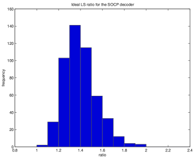
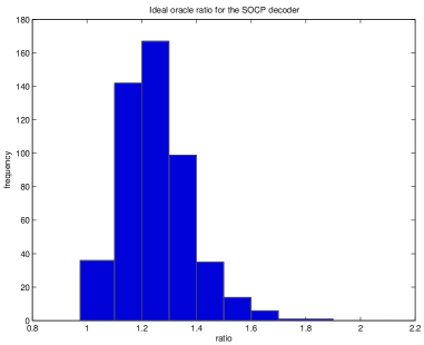
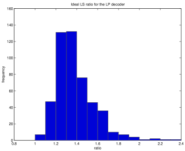
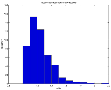
Figure 1: Statistics of the ratios (4.1) $\rho^{\text{Ideal}}$ (first column) and $\rho^{\text{Oracle}}$ (second column) which compare the performance of the proposed decoders with that of ideal strategies which assume either exact knowledge of the gross errors or exact knowledge of their locations. The first row shows the performance of the SOCP decoder, the second that of the LP decoder.

	median of $\rho^{\text{Ideal}}$	mean of $\rho^{\text{Ideal}}$	median of $\rho^{\text{Oracle}}$	mean of $\rho^{\text{Oracle}}$
SOCP decoder	1.386	1.401	1.241	1.253
LP decoder	1.346	1.386	1.212	1.239

Table 1: Summary statistics of the ratios $\rho^{\text{Ideal}}$ and $\rho^{\text{Oracle}}$ (4.1) for the Gaussian coding matrix.

We also repeated the same experiment but with a coding matrix $A$ consisting of $n=256$ randomly sampled columns of the $512\times 512$ discrete Fourier transform, and obtained very similar results. The results are presented in Figure 2 and summarized in Table 2. The numbers are remarkably close to our earlier findings and again both our methods work extremely well (again the LP decoder is a tiny bit more accurate). This experiment is of special interest since it suggests that one can apply our decoding algorithms to very large data vectors, e.g. with sizes ranging in the hundred of thousands. The reason is that one can use off-the-shelf interior point algorithms which only need to be able to apply $A$ or $A^{*}$ to arbitrary vectors (and never need to manipulate the entries of $A$ or even store them). When $A$ is a partial Fourier transform, one can evaluate $Ax$ and $A^{*}y$ by means of the FFT and, hence, this is well suited for very large problems. See [2] for very large scale experiments of a similar flavor.

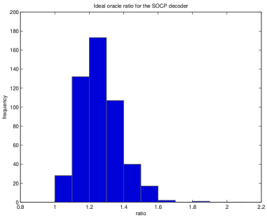
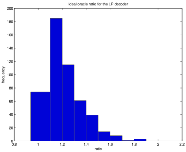
Figure 2: Statistics of the ratios $\rho^{\text{Oracle}}$ for the SOCP decoder (first column) and the LP decoder (second column) in the case where the coding matrix is a partial Fourier transform.

	median of $\rho^{\text{Ideal}}$	mean of $\rho^{\text{Ideal}}$	median of $\rho^{\text{Oracle}}$	mean of $\rho^{\text{Oracle}}$
SOCP decoder	1.390	1.401	1.244	1.262
LP decoder	1.337	1.375	1.195	1.230

Table 2: Summary statistics of the ratios $\rho^{\text{Ideal}}$ and $\rho^{\text{Oracle}}$ (4.1) for the Fourier coding matrix.

5 Proofs

In this section, we prove all of our results. We begin with some preliminaries which will be used throughout, then prove the claims about the SOCP decoder, and end this section with the LP decoder. Our work builds on [4] and [7].

5.1 Preliminaries

We shall make extensive use of two simple lemmas that we now record.

Lemma 5.1

Let $Y_{d}\sim\chi^{2}_{d}$ be distributed as a chi-squared random variable with $d$ degrees of freedom. Then for each $t>0$

$${\hbox{\bf P}}(Y_{d}-d\geq t\,\sqrt{2d}+t^{2})\leq e^{-t^{2}/2}\quad\text{ and }\quad{\hbox{\bf P}}(Y_{d}-d\leq-t\,\sqrt{2d})\leq e^{-t^{2}/2}.$$ (5.1)

This is fairly standard [17], see also [16] for very slightly refined estimates. A consequence of these large deviation bounds is the estimate below.

Lemma 5.2

Let $U=(u_{1},u_{2},\ldots,u_{m})$ be a vector uniformly distributed on the unit sphere in $m$ dimensions. Let $Z_{n}=u_{1}^{2}+\ldots+u_{n}^{2}$ be the squared length of the first $n$ components of $u$. Then for each $t\leq 1/2$

$${\hbox{\bf P}}\left(Z_{n}\leq\frac{n}{m}\,(1-t)\right)\leq e^{-nt^{2}/16}+e^{-mt^{2}/24}.$$ (5.2)

Proof Suppose $X_{1},X_{2},\ldots,X_{m}$ are i.i.d. $N(0,1)$. Then the distribution of $U$ is that of the vector $X/\|X\|_{\ell_{2}}$ and, therefore, the law of $Z_{n}$ is that of $Y_{n}/Y_{m}$, where $Y_{k}=\sum_{j\leq k}X_{j}^{2}$. Define the events $A_{\varepsilon}=\{Y_{m}\geq(1+\varepsilon)m\}$ for some $\varepsilon>0$ and $B_{t}=\{Y_{n}/Y_{m}\leq n/m(1-t)\}$. We have

$${\hbox{\bf P}}(B_{t}) ={\hbox{\bf P}}(B_{t}\,|\,A_{\varepsilon}^{c})\,{\hbox{\bf P}}(A_{\varepsilon}^{c})+{\hbox{\bf P}}(B_{t}\,|\,A_{\varepsilon})\,{\hbox{\bf P}}(A_{\varepsilon})$$

$$\leq{\hbox{\bf P}}(Y_{n}\leq n(1-t)(1+\varepsilon))+{\hbox{\bf P}}(Y_{m}\geq(1+\varepsilon)m).$$

With $\varepsilon=t/2$, this gives $n(1-t)(1+\varepsilon)\leq n(1-t/2)$ and thus

$${\hbox{\bf P}}(Z_{n}\leq n/m(1-t)) \leq{\hbox{\bf P}}(Y_{n}\leq n(1-t/2))+{\hbox{\bf P}}(Y_{m}\geq(1+\varepsilon)m)$$

$$\leq e^{-nt^{2}/16}+e^{-\gamma^{2}m/2},$$

which follows from (5.1), where $\gamma$ obeys $t/2=\gamma\sqrt{2}+\gamma^{2}$. For $t\leq 1/2$, $\gamma\leq 1/2\sqrt{3}$ (for small values of $t$, $\gamma\approx t/2\sqrt{2}$) and the conclusion follows.  

5.2 The SOCP decoder

For a matrix $\Phi$, define the sequences $(a_{k})$ and $(b_{k})$ as respectively the largest and smallest numbers obeying

$$a_{k}\|x\|_{\ell_{2}}\leq\|\Phi x\|_{\ell_{2}}\leq b_{k}\|x\|_{\ell_{2}},$$ (5.3)

for all $k$-sparse vectors. In other words, if we list all the singular values of all the submatrices of $\Phi$ with $k$ columns, $a_{k}$ is the smallest element from that list and $b_{k}$ the largest. Note of course the resemblance with (2.6)—only this is slightly more general. We now adapt an important result from [4].

Lemma 5.3 (adapted from [4])

Set $\Phi\in{{\mathbb{R}}}^{r\times m}$ and let $(a_{k})$ and $(b_{k})$ be the restricted extremal singular values of $\Phi$ as in (5.3). Any point $\tilde{x}\in{{\mathbb{R}}}^{m}$ obeying

$$\|\tilde{x}\|_{\ell_{1}}\leq\|x\|_{\ell_{1}},\quad\text{ and }\quad\|\Phi\tilde{x}-\Phi x\|_{\ell_{2}}\leq 2\varepsilon,$$ (5.4)

also obeys

$$\|\tilde{x}-x\|_{\ell_{2}}\leq\frac{\sqrt{6}\,\varepsilon}{a_{3k}(\Phi)-\frac{1}{\sqrt{2}}\,b_{2k}(\Phi)},$$ (5.5)

provided that $x$ is $k$-sparse with $k$ such that $a_{3k}(\Phi)-\frac{1}{\sqrt{2}}\,b_{2k}(\Phi)>0$.

The proof follows the same steps as that of Theorem 1.1 in [4], and is omitted. In particular, it follows from (2.6) in the aforementioned reference with $M=2|T_{0}|$ and $a_{M+|T_{0}|}$ (resp. $b_{M}$) in place of $\sqrt{1-\delta_{|T_{0}|+M}}$ (resp. $\sqrt{1+\delta_{M}})$ in the definition of $C_{|T_{0}|,M}$.

5.2.1 Proof of Theorem 2.2

Recall that the solution $(\hat{x},\hat{z})$ to $(P_{2})$ obeys (2.4) where $\hat{e}$ is the solution to $(P^{\prime}_{2})$. Replacing $y$ in (2.4) with $Ax+e+z$ gives

$$\hat{x}-x =(A^{*}A)^{-1}A^{*}(e-\hat{e})+(A^{*}A)^{-1}A^{*}z$$

$$=(A^{*}A)^{-1}A^{*}(e-\hat{e})+x^{\text{Ideal}}-x,$$ (5.6)

and since $A^{*}A=I$,

$$\|\hat{x}-x\|_{\ell_{2}}\leq\|A^{*}(e-\hat{e})\|_{\ell_{2}}+\|x^{\text{Ideal}}-x\|_{\ell_{2}}.$$

To prove (2.7), it then suffices to show that $\|e-\hat{e}\|_{\ell_{2}}\leq\frac{C\,\varepsilon}{\sqrt{1-\frac{n}{m}}}$ since the 2-norm of $A^{*}$ is at most 1.

By assumption $\|Q^{*}(y-e)\|_{\ell_{2}}=\|Q^{*}z\|_{\ell_{2}}\leq\varepsilon$ and thus, $e$ is feasible for $(P^{\prime}_{2})$ which implies $\|\hat{e}\|_{\ell_{1}}\leq\|e\|_{\ell_{1}}$. Moreover,

$$\|Q^{*}e-Q^{*}\hat{e}\|_{\ell_{2}}\leq\|Q^{*}(y-e)\|_{\ell_{2}}+\|Q^{*}(y-\hat{e})\|_{\ell_{2}}\leq 2\varepsilon.$$

We then apply Lemma 5.3 (with $\Phi=Q^{*}$) and obtain

$$\|e-\hat{e}\|_{\ell_{2}}\leq\frac{\sqrt{6}\,\varepsilon}{a_{3k}(Q^{*})-\frac{1}{\sqrt{2}}\,b_{2k}(Q^{*})}.$$ (5.7)

Now since the $m\times m$ matrix obtained by concatenating the columns of $A$ and $Q$ is an isometry, we have

$$\|A^{*}x\|_{\ell_{2}}^{2}+\|Q^{*}x\|_{\ell_{2}}^{2}=\|x\|_{\ell_{2}}^{2}\quad\forall x\in{{\mathbb{R}}}^{m},$$

whence

$$a^{2}_{k}(Q^{*}) =1-b^{2}_{k}(A^{*}),$$

$$b^{2}_{k}(Q^{*}) =1-a^{2}_{k}(A^{*}).$$

Assuming that $a_{3k}(Q^{*})\geq\frac{1}{\sqrt{2}}b_{2k}(Q^{*})$, we deduce from (5.7) that

$$\|e-\hat{e}\|_{\ell_{2}}\leq\sqrt{6}\,\varepsilon\cdot\frac{a_{3k}(Q^{*})+\frac{1}{\sqrt{2}}b_{2k}(Q^{*})}{1-b^{2}_{3k}(A^{*})-\frac{1}{2}(1-a^{2}_{2k}(A^{*}))}\leq 2\sqrt{6}\varepsilon\cdot\frac{a_{3k}(Q^{*})}{\frac{1}{2}+\frac{1}{2}a^{2}_{2k}(A^{*})-b_{3k}^{2}(A^{*})}.$$ (5.8)

Recall that $(\delta_{k})$ are the restricted isometry constants of $\sqrt{\frac{m}{n}}\,A^{*}$, and observe that by definition for each $k=1,2,\ldots$,

$$a_{k}^{2}(A^{*})\geq\frac{n}{m}(1-\delta_{k}),\qquad b^{2}_{k}(A^{*})\leq\frac{n}{m}(1+\delta_{k}).$$

It follows that the denominator on the right-hand side of (5.8) is greater or equal to

$$\frac{1}{2}+\frac{n}{2m}(1-\delta_{2k})-\frac{n}{m}(1+\delta_{3k})=\frac{1}{2}\left(1-\frac{n}{m}\right)-\frac{n}{m}\left(\delta_{3k}+\frac{1}{2}\delta_{2k}\right).$$

Now suppose that for some $0<c<1$,

$$\delta_{3k}+\frac{1}{2}\delta_{2k}\leq\frac{c}{2}\cdot\left(\frac{m}{n}-1\right).$$

This automatically implies $a_{3k}(Q^{*})\geq\frac{1}{\sqrt{2}}b_{2k}(Q^{*})$, and the denominator on the right-hand side of (5.8) is greater or equal to $\frac{1}{2}(1-c)(1-\frac{n}{m})$. The numerator obeys

$$a^{2}_{3k}(Q^{*})=1-b^{2}_{3k}(A^{*})\leq 1-a^{2}_{3k}(A^{*})\leq 1-(1-\delta_{3k})\frac{n}{m}.$$

Since $\frac{n}{m}\,\delta_{3k}\leq\frac{c}{2}(1-\frac{n}{m})$, we also have $a^{2}_{3k}(Q^{*})\leq(1+\frac{c}{2})(1-\frac{n}{m})$. In summary, (5.8) gives

$$\|e-\hat{e}\|_{\ell_{2}}\leq C_{2}\cdot\frac{\varepsilon}{\sqrt{1-\frac{n}{m}}},$$

where one can take $C_{2}$ as $4\sqrt{6(1+c/2)}/(1-c)$. This establishes the first part of the claim.

We now turn to the second part of the theorem and argue that if the orthonormal columns of $A$ are chosen uniformly at random, the error bound (2.7) is valid as long as we have a constant fraction of gross errors. Put $r=m-n$ and let $X$ be an $m$ by $r$ matrix with independent Gaussian entries with mean 0 and variance $1/m$. Consider now the reduced singular value decomposition of $X$

$$X=U\Sigma V^{*},\quad U\in{{\mathbb{R}}}^{m\times r}\text{ and }\Sigma,V\in{{\mathbb{R}}}^{r\times r}.$$

Then the columns of $U$ are $r$ orthonormal vectors selected uniformly at random and thus $U$ and $Q$ have the same distribution. Thus we can think of $Q$ as being the left singular vectors of a Gaussian matrix $X$ with independent entries. From now on, we identify $U$ with $Q$. Observe now that

$$\|X^{*}(\hat{e}-e)\|_{\ell_{2}}=\|V\Sigma Q^{*}(\hat{e}-e)\|_{\ell_{2}}=\|\Sigma Q^{*}(\hat{e}-e)\|_{\ell_{2}}\leq\sigma_{1}(X)\,\|Q^{*}(\hat{e}-e)\|_{\ell_{2}},$$

where $\sigma_{1}(X)$ is the largest singular value of $X$. The singular values of Gaussian matrices are well concentrated and a classical result [10] shows that

$${\hbox{\bf P}}\left(\sigma_{1}(X)>1+\sqrt{\frac{r}{m}}+t\right)\leq e^{-mt^{2}/2}.$$ (5.9)

By choosing $t=1$ in the above formula, we have

$$\|X^{*}(\hat{e}-e)\|_{\ell_{2}}\leq 3\|Q^{*}(\hat{e}-e)\|_{\ell_{2}}\leq 6\varepsilon$$

with probability at least $1-e^{-m/2}$ since $\|Q^{*}(\hat{e}-e)\|_{\ell_{2}}\leq 2\epsilon$. We now apply Lemma 5.3 with $\Phi=X^{*}$, which gives

$$\|e-\hat{e}\|_{\ell_{2}}\leq\frac{3\sqrt{6}\,\varepsilon}{a_{3k}(X^{*})-\frac{1}{\sqrt{2}}\,b_{2k}(X^{*})}=\sqrt{\frac{m}{r}}\cdot\frac{3\sqrt{6}\,\varepsilon}{a_{3k}(Y^{*})-\frac{1}{\sqrt{2}}\,b_{2k}(Y^{*})},$$ (5.10)

where $Y=\sqrt{\frac{m}{r}}X$. The theorem is proved since it is well known that if $k\leq c_{0}\cdot r/\log(m/r)$ for some constant $c_{0}$, we have $a_{3k}(Y^{*})-\frac{1}{\sqrt{2}}\,b_{2k}(Y^{*})\geq c_{1}$ with probability at least $1-O(e^{-\gamma^{\prime}r})$ for some universal constants $c_{1}$ and $\gamma$; this follows from available bounds on the restricted isometry constants of Gaussian matrices [8, 6, 12, 21].

5.2.2 Proof of Corollary 2.3

First, we can just assume that $\sigma=1$ as the general case is treated by a simple rescaling. Put $r=m-n$. Since the random vector $z$ follows a multivariate normal distribution with mean zero and covariance matrix $I_{m}$ ($I_{m}$ is the identity matrix in $m$ dimensions), $Q^{*}z$ is also multivariate normal with mean zero and covariance matrix $Q^{*}Q=I_{r}$. Consequently, $\|Q^{*}z\|_{\ell_{2}}^{2}$ is distributed as a chi-squared variable with $r$ degrees of freedom. Pick $\lambda=\gamma\,\sqrt{r}$ in (5.1), and obtain

$${\hbox{\bf P}}\left(\|Q^{*}z\|^{2}_{\ell_{2}}\geq(1+\gamma\sqrt{2}+\gamma^{2})r\right)\leq e^{-\gamma^{2}r/2}.$$

With $t=\gamma\sqrt{2}+\gamma^{2}$ so that $\gamma=(\sqrt{1+2t}-1)/\sqrt{2}$, we have $\|Q^{*}z\|_{\ell_{2}}\leq\sqrt{r(1+t)}$ with probability at least $1-e^{-\gamma^{2}(m-n)/2}$. On this event, Theorem 2.2 asserts that

$$\|\hat{x}-x\|_{\ell_{2}}\leq C\,\sqrt{m(1+t)}+\|x-x^{\text{Ideal}}\|_{\ell_{2}}.$$

This essentially concludes the proof of the corollary since the size of $\|x-x^{\text{Ideal}}\|_{\ell_{2}}$ is about $\sqrt{n}$. Indeed, $\|x-x^{\text{Ideal}}\|^{2}_{\ell_{2}}=\|A^{*}z\|^{2}_{\ell_{2}}\sim\chi^{2}_{n}$ as observed earlier. As a consequence, for each $t_{0}>0$, we have $\|x-x^{\text{Ideal}}\|_{\ell_{2}}\leq\sqrt{n(1+t_{0})}\cdot\sigma$ with probability at least $1-e^{-\gamma_{0}^{2}n/2}$, where $\gamma_{0}$ is the same function of $t_{0}$ as before. Selecting $t_{0}$ as $t_{0}=m/n$, say, gives the result.

5.3 The LP decoder

Before we begin, we introduce the number $\theta_{k,k^{\prime}}$ of a matrix $\Phi\in{{\mathbb{R}}}^{r\times m}$ for $k+k^{\prime}\leq m$ called the $k,k^{\prime}$-restricted orthogonality constants. This is the smallest quantity such that

$$|\langle\Phi v,\Phi v^{\prime}\rangle|\leq\theta_{k,k^{\prime}}\cdot\|v\|_{\ell_{2}}\,\|v^{\prime}\|_{\ell_{2}}$$ (5.11)

holds for all $k$ and $k^{\prime}$-sparse vectors supported on disjoint sets. Small values of restricted orthogonality constants indicate that disjoint subsets of columns span nearly orthogonal subspaces. The following lemma which relates the number $\theta_{k,k^{\prime}}$ to the extremal singular values will prove useful.

Lemma 5.4

For any matrix $\Phi\in{{\mathbb{R}}}^{r\times m}$, we have

$$\theta_{k,k^{\prime}}(\Phi)\leq\frac{1}{2}\,(b_{k+k^{\prime}}^{2}(\Phi)-a^{2}_{k+k^{\prime}}(\Phi)).$$

Proof Consider two vectors $v$ and $v^{\prime}$ which are respectively $k$ and $k^{\prime}$-sparse. By definition we have

$$2a^{2}_{k+k^{\prime}}(\Phi) \leq\|\Phi v+\Phi v^{\prime}\|_{\ell_{2}}^{2}\leq 2b^{2}_{k+k^{\prime}}(\Phi),$$

$$2a_{k+k^{\prime}}^{2}(\Phi) \leq\|\Phi v-\Phi v^{\prime}\|_{\ell_{2}}^{2}\leq 2b^{2}_{k+k^{\prime}}(\Phi),$$

and the conclusion follows from the parallelogram identity

$$|\langle\Phi v,\Phi v^{\prime}\rangle|=\frac{1}{4}\left|\|\Phi v+\Phi v^{\prime}\|_{\ell_{2}}^{2}-\|\Phi v-\Phi v^{\prime}\|_{\ell_{2}}^{2}\right|\leq\frac{1}{2}\,(b_{k+k^{\prime}}^{2}(\Phi)-a^{2}_{k+k^{\prime}}(\Phi)).$$

 

The argument underlying Theorem 3.1 uses an intermediate result whose proof may be found in the Appendix. Here and in the remainder of this paper, $x_{I}$ is the restriction of the vector $x$ to an index set $I$, and for a matrix $X$, $X_{I}$ is the submatrix formed by selecting the columns of $X$ with indices in $I$.

Lemma 5.5

Let $\Phi$ be an $r\times m$-dimensional matrix and suppose $T_{0}$ is a set of cardinality $k$. For a vector $h\in{{\mathbb{R}}}^{m}$, we let $T_{1}$ be the $k^{\prime}$ largest positions of $h$ outside of $T_{0}$. Put $T_{01}=T_{0}\cup T_{1}$. Then

$$\|h_{T_{01}}\|_{\ell_{2}}\leq\frac{1}{a^{2}_{k+k^{\prime}}(\Phi)}\,\|\Phi^{*}_{T_{01}}\Phi h\|_{\ell_{2}}+\frac{\theta_{k^{\prime},k+k^{\prime}}(\Phi)}{a^{2}_{k+k^{\prime}}(\Phi)\,\sqrt{k^{\prime}}}\,\|h_{T_{0}^{c}}\|_{\ell_{1}}$$ (5.12)

and

$$\|h\|^{2}_{\ell_{2}}\leq\|h_{T_{01}}\|^{2}_{\ell_{2}}+\frac{1}{k^{\prime}}\|h_{T_{0}^{c}}\|_{\ell_{1}}^{2}.$$ (5.13)

5.3.1 Proof of Theorem 3.1

Just as before, it suffices to show that $\|e-\hat{e}\|_{\ell_{2}}\leq C\sqrt{k}\cdot\lambda\cdot(1-n/m)^{-1}$. Set $h=\hat{e}-e$ and let $T_{0}$ be the support of $e$ (which has size $k$). Because $e$ is feasible for $(P^{\prime}_{\infty})$ we have on the one hand $\|\hat{e}\|_{\ell_{1}}\leq\|e\|_{\ell_{1}}$, which gives

$$\|e_{T_{0}}\|_{\ell_{1}}-\|h_{T_{0}}\|_{\ell_{1}}+\|h_{T_{0}^{c}}\|_{\ell_{1}}\leq\|e+h\|_{\ell_{1}}\leq\|e\|_{\ell_{1}}\Rightarrow\|h_{T_{0}^{c}}\|_{\ell_{1}}\leq\|h_{T_{0}}\|_{\ell_{1}}.$$

Note that this has an interesting consequence since

$$\|h_{T_{0}^{c}}\|_{\ell_{1}}\leq\|h_{T_{0}}\|_{\ell_{1}}\leq\sqrt{k}\cdot\|h_{T_{0}}\|_{\ell_{2}}$$ (5.14)

by Cauchy Schwarz. On the other hand

$$\|QQ^{*}h\|_{\ell_{\infty}}\leq\|QQ^{*}(\hat{e}-y)\|_{\ell_{\infty}}+\|QQ^{*}(y-e)\|_{\ell_{\infty}}\leq 2\lambda.$$ (5.15)

The ingredients are now in place to establish the claim. We set $k^{\prime}=k$, apply Lemma (5.5) with $\Phi=Q^{*}$ to the vector $h=\hat{e}-e$, and obtain

$$\|h\|_{\ell_{2}}\leq\sqrt{2}\,\|h_{T_{01}}\|_{\ell_{2}},\quad\text{ and }\quad\|h_{T_{01}}\|_{\ell_{2}}\leq\frac{1}{a^{2}_{2k}(Q^{*})-\theta_{k,2k}(Q^{*})}\,\|Q_{T_{01}}Q^{*}h\|_{\ell_{2}}.$$ (5.16)

Since each component of $Q_{T_{01}}Q^{*}h$ is at most equal to $2\lambda$, see (5.15), we have $\|Q_{T_{01}}Q^{*}h\|_{\ell_{2}}\leq\sqrt{2k}\cdot 2\lambda$. We then conclude from Lemma 5.4 that

$$\|h\|_{\ell_{2}}\leq 2\sqrt{k}\cdot\frac{2\lambda}{a^{2}_{2k}(Q^{*})+\frac{1}{2}a^{2}_{3k}(Q^{*})-\frac{1}{2}b^{2}_{3k}(Q^{*})}.$$ (5.17)

For each $k$, recall the relations $a_{k}^{2}(Q^{*})=1-b_{k}^{2}(A^{*})$ and $b_{k}^{2}(Q^{*})=1-a_{k}^{2}(A^{*})$ which give

$$\|h\|_{\ell_{2}}\leq 4\sqrt{k}\cdot\frac{\lambda}{D},\qquad D:=1-b^{2}_{2k}(A^{*})-\frac{1}{2}b^{2}_{3k}(A^{*})+\frac{1}{2}a^{2}_{3k}(A^{*}).$$

Now just as before, it follows from our definitions that for each $k$, $b^{2}_{k}(A^{*})\leq\frac{n}{m}(1+\delta_{k})$ and $a^{2}_{k}(A^{*})\geq\frac{n}{m}(1-\delta_{k})$. These inequalities imply

$$D\geq 1-\frac{n}{m}(1+\delta_{2k}+\delta_{3k}).$$

Therefore, if one assumes that

$$\delta_{2k}+\delta_{3k}\leq c\left(\frac{m}{n}-1\right),$$

for some fixed constant $0<c<1$, then

$$\|e-\hat{e}\|_{\ell_{2}}=\|h\|_{\ell_{2}}\leq\frac{4\sqrt{k}}{1-c}\cdot\frac{\lambda}{1-\frac{n}{m}}.$$

This establishes the first part of the theorem.

We turn to the second part of the claim; if the orthonormal columns of $A$ are chosen uniformly at random, we show that the error bound (3.5) is valid with large probability as long as we have a constant fraction of gross errors. The same argument as before (albeit for a general value of $k^{\prime}$) gives

$$\|h\|_{\ell_{2}}\leq\frac{k+k^{\prime}}{\sqrt{k^{\prime}}}\cdot\frac{2\lambda}{D},\qquad D:=a^{2}_{k+k^{\prime}}(Q^{*})+\frac{1}{2}\sqrt{\frac{k}{k^{\prime}}}(a^{2}_{k+2k^{\prime}}(Q^{*})-b^{2}_{k+2k^{\prime}}(Q^{*})).$$ (5.18)

so that this is really a question about the extremal singular values of random orthogonal projections when restricted to sparse inputs.

Put $r=m-n$ and let $X$ be an $m$ by $r$ matrix with independent Gaussian entries with mean 0 and variance $1/m$. Recall the QR factorization of $X$.

$$X=Q^{\prime}R,\quad Q^{\prime}\in{{\mathbb{R}}}^{m\times r},\,R\in{{\mathbb{R}}}^{r\times r},$$

where $R$ is upper triangular. The columns of $Q^{\prime}$ are $r$ orthonormal vectors selected uniformly at random and thus, $Q$ and $Q^{\prime}$ have the same distribution so that we can think of $Q$ as being the $Q$-factor in the QR factorization of $X$. Also observe that $\sigma_{j}(X)=\sigma_{j}(R)$, $1\leq j\leq r$, i.e. the nonzero singular values of $R$ and $X$ coincide. It follows from

$$v^{*}XX^{*}v=v^{*}QRR^{*}Q^{*}v$$

(which is valid for all $v\in R^{m}$) that

$$\sigma_{r}(X)\|Q^{*}v\|_{\ell_{2}}\leq\|X^{*}v\|_{\ell_{2}}\leq\sigma_{1}(X)\|Q^{*}v\|_{\ell_{1}}.$$

Applying the above inequalities to $k$-sparse vectors gives

$$b_{k}(Q^{*}) \leq\frac{1}{\sigma_{r}(X)}b_{k}(X^{*}),$$

$$a_{k}(Q^{*}) \geq\frac{1}{\sigma_{1}(X)}a_{k}(X^{*}).$$

The point is that the extremal singular values $(a_{k}(X^{*}),b_{k}(X^{*}))_{1\leq k\leq r}$ are perhaps easier to study than those of $Q^{*}$.

Indeed, classical results from random matrix theory [10, 18] assert that for each $t>0$,

$${\hbox{\bf P}}\left(\sigma_{1}(X^{*})>1+(1+t)\sqrt{\frac{r}{m}}\right) \leq e^{-rt^{2}/2},$$ (5.19)

$${\hbox{\bf P}}\left(\sigma_{r}(X^{*})<1-(1+t)\sqrt{\frac{r}{m}}\right) \leq e^{-rt^{2}/2}.$$ (5.20)

These inequalities can be specialized to $r\times k$ submatrices of $X$, and taking the union bound also show that for each $t>0$

$${\hbox{\bf P}}\left(\sqrt{\frac{m}{r}}\,b_{k}(X^{*})>1+\sqrt{\frac{k}{r}}+t\right) \leq\binom{m}{k}\,e^{-rt^{2}/2},$$ (5.21)

$${\hbox{\bf P}}\left(\sqrt{\frac{m}{r}}\,a_{k}(X^{*})<1-\sqrt{\frac{k}{r}}-t\right) \leq\binom{m}{k}\,e^{-rt^{2}/2}.$$ (5.22)

We use these estimates to bound below the denominator $D$ in (5.18). We first study the case where $r\leq m/16$ and in the sequel, we will denote $\sqrt{k/k^{\prime}}$ by $\rho$. First, pick $t=1/3$ in (5.19)–(5.20). Then the event

$$E_{0}:=\{2/3\leq\sigma_{r}(X)\leq\sigma_{1}(X)\leq 4/3\}$$

has probability at least $1-2e^{-r/18}$. On this event, the denominator $D$ in (5.18) obeys

$$D\geq(3/4)^{2}a^{2}_{k+k^{\prime}}(X^{*})-(3/2)^{2}\frac{\rho}{2}b^{2}_{k+2k^{\prime}}(X^{*})=\frac{9}{16}\,(a^{2}_{k+k^{\prime}}(X^{*})-2\rho\,b^{2}_{k+2k^{\prime}}(X^{*})).$$

Second, selecting $t=1/8$ in (5.21) and (5.22) shows that the events $E_{1}$ and $E_{2}$ respectively equal to

$$\sqrt{\frac{m}{r}}a_{k+k^{\prime}}(X^{*})\geq\frac{7}{8}-\sqrt{\frac{k+k^{\prime}}{r}}\quad\text{ and }\quad\sqrt{\frac{m}{r}}b_{k+2k^{\prime}}(X^{*})>\frac{9}{8}+\sqrt{\frac{k+2k^{\prime}}{r}}$$

have probability at least $1-\binom{m}{k+k^{\prime}}e^{-r/128}$ and $1-\binom{m}{k+2k^{\prime}}e^{-r/128}$. Third, select $k^{\prime}$ to be the smallest integer so that $\rho=\sqrt{k/k^{\prime}}\leq 1/8$. Combining these facts gives

$${\hbox{\bf P}}\left(D\geq\frac{9r}{16m}\,\left[\left(\frac{7}{8}-\sqrt{\frac{k+k^{\prime}}{r}}\right)^{2}-\frac{1}{4}\left(\frac{9}{8}+\sqrt{\frac{k+2k^{\prime}}{r}}\right)^{2}\right]\right)\geq 1-\eta,$$

where $\eta=2\binom{m}{k+2k^{\prime}}e^{-r/128}+2e^{-r/18}$. Elementary calculations show that

$$\left(\frac{7}{8}-\sqrt{\frac{k+k^{\prime}}{r}}\right)-\frac{1}{2}\left(\frac{9}{8}+\sqrt{\frac{k+2k^{\prime}}{r}}\right)\geq\frac{1}{16}\quad\text{if}\quad\sqrt{\frac{k+k^{\prime}}{r}}+\frac{1}{2}\sqrt{\frac{k+2k^{\prime}}{r}}\leq\frac{1}{4},$$

and

$$\left(\frac{7}{8}-\sqrt{\frac{k+k^{\prime}}{r}}\right)-\frac{1}{2}\left(\frac{9}{8}+\sqrt{\frac{k+2k^{\prime}}{r}}\right)\geq 1$$

under the same condition. In summary, $D\geq{9r}/{256m}$ with probability at least $1-\eta$ provided that

$$\sqrt{\frac{k+k^{\prime}}{r}}+\frac{1}{2}\sqrt{\frac{k+2k^{\prime}}{r}}\leq\sqrt{\frac{k}{r}}\cdot\left(\sqrt{66}+\frac{1}{2}\sqrt{131}\right)\leq\frac{1}{4}$$

since $k^{\prime}/k\leq 65$. Finally $k+2k^{\prime}\leq 131k$ and assuming $131k\leq m/2$, we also have

$$\log\binom{m}{k+2k^{\prime}}\leq\log\binom{m}{131k}\leq 131k\left[1+\log\frac{m}{131k}\right].$$ (5.23)

In other words, $D\geq{9r}/{256m}$ with probability at least $1-2e^{-r/256}-2e^{-r/18}$ as long as the right-hand side of (5.23) is less or equal to $r/256$. It follows from $\eqref{eq:almost3}$ that with at least the same probability, $\|\hat{e}-e\|_{\ell_{2}}\leq C_{1}\cdot(m/r)\cdot\sqrt{k}\cdot\lambda$ and hence, one can correct a constant fraction of errors (the fraction depends on $n/m$ of course) in the case where $r\leq m/16$.

It remains to argue that the result is valid when $r\geq m/16$. Here, the denominator $D$ in (5.18) obeys

$$D\geq b_{k+2k^{\prime}}^{2}(Q^{*})-\rho/2\geq b_{1}^{2}(Q^{*})-\rho/2.$$

Let $Z_{r}$ be the squared $\ell_{2}$ norm of the first column of $Q^{*}$, i.e. $Z_{r}=(QQ^{*})_{1,1}$. We have $b_{1}^{2}(Q^{*})\geq Z_{r}$ and moreover, Lemma 5.2 proved that

$${\hbox{\bf P}}(Z_{r}<3r/4m)\leq 2e^{-\gamma_{0}^{2}r/2}$$

for some constant $\gamma_{0}>0$. Pick $k^{\prime}$ to be the smallest integer so that $\rho=\sqrt{k/k^{\prime}}\leq r/m$. Then $D\geq r/4m$, and we conclude that $\|\hat{e}-e\|_{\ell_{2}}\leq C\cdot(m/r)\cdot\sqrt{k}\cdot\lambda$ with probability at least $1-2e^{-\gamma_{0}^{2}r/2}$. To be complete, the condition on $k$ is $k+2k^{\prime}\leq r$ which is satisfied if $k(3+(m/r)^{2})\leq r$ or equivalently $k\leq\rho_{0}\cdot m$ with $\rho_{0}=r/m\cdot(1+(m/r)^{2})^{-1}$.

5.3.2 Proof of Corollary 3.2

First, we can just assume that $\sigma=1$ as the general case is treated by a simple rescaling. The random vector $QQ^{*}z$ follows a multivariate normal distribution with mean zero and covariance matrix $QQ^{*}$. In particular $(QQ^{*}z)_{i}\sim N(0,s^{2}_{i})$, where $s_{i}^{2}=(QQ^{*})_{i,i}$. This implies that $z^{\prime}_{i}=(QQ^{*}z)_{i}/s_{i}$ is standard normal with density $\phi(t)=(2\pi)^{-1/2}e^{-t^{2}/2}$. For each $i$, ${\hbox{\bf P}}(|z^{\prime}_{i}|>t)\leq\phi(t)/t$ and thus

$${\hbox{\bf P}}\left(\sup_{1\leq i\leq m}|z^{\prime}_{i}|\geq t\right)\leq 2m\cdot\phi(t)/t.$$

With $t=\sqrt{2\log m}$, this gives ${\hbox{\bf P}}(\sup_{1\leq i\leq m}|z^{\prime}_{i}|\geq\sqrt{2\log m})\leq 1/\sqrt{\pi\log m}$. Better bounds are possible but we will not pursue these refinements here. Observe now that $s_{i}^{2}=\|Q_{i,\cdot}\|^{2}_{\ell_{2}}=1-\|A_{i,\cdot}\|^{2}_{\ell_{2}}$, and since $\lambda_{i}=\sqrt{2\log m}\,\|Q_{i,\cdot}\|_{\ell_{2}}$, we have that

$$|QQ^{*}z_{i}|\leq\lambda_{i},\quad\forall i$$ (5.24)

with probability at least $1-1/\sqrt{\pi\log m}$.

On the event (5.24), Theorem 3.1 then shows that

$$\|\hat{x}-x\|_{\ell_{2}}\leq C\,\sqrt{k}\cdot(m/r)\cdot\max_{i}|\lambda_{i}|+\|x-x^{\text{Ideal}}\|_{\ell_{2}}.$$ (5.25)

We claim that

$$\frac{\max_{i}|\lambda_{i}|}{\sqrt{2\log m}}=\max_{i}\|Q_{i,\cdot}\|_{\ell_{2}}\leq\sqrt{\frac{3r}{m}}$$ (5.26)

with probability at least $1-2e^{-\gamma m}$ for some positive constant $\gamma$. Combining (5.25) and (5.26) yields

$$\|\hat{x}-x\|_{\ell_{2}}\leq 2C\cdot\sqrt{\frac{m\log m}{m-n}}\cdot\sqrt{k}+\|x-x^{\text{Ideal}}\|_{\ell_{2}}.$$

This would essentially conclude the proof of the corollary since the size of $\|x-x^{\text{Ideal}}\|_{\ell_{2}}$ is about $\sqrt{n}$. Exact bounds for $\|x-x^{\text{Ideal}}\|_{\ell_{2}}$ are found in the proof of Corollary 2.3 and we do not repeat the argument.

It remains to check why (5.26) is true. For $r\geq m/3$ and since $\|Q_{i,\cdot}\|_{\ell_{2}}\leq 1$, the claim holds with probability 1 because $3r/m\geq 1$! For $r\leq m/3$, it follows from $\|Q_{i,\cdot}\|^{2}_{\ell_{2}}+\|A_{i,\cdot}\|^{2}_{\ell_{2}}=1$ that

$${\hbox{\bf P}}\left(\max_{i}\|Q_{i,\cdot}\|^{2}_{\ell_{2}}\geq\frac{2r}{m}\right)={\hbox{\bf P}}\left(\min_{i}\|A_{i,\cdot}\|^{2}_{\ell_{2}}\leq\frac{n}{m}\left(1-\frac{r}{n}\right)\right)\leq m\,{\hbox{\bf P}}\left(\|A_{1,\cdot}\|^{2}_{\ell_{2}}\leq\frac{n}{m}\left(1-\frac{r}{n}\right)\right).$$

The claim follows by applying Lemma 5.2 since $r/n\leq 1/2$.

6 Discussion

We have introduced two decoding strategies for recovering a block $x\in{{\mathbb{R}}}^{n}$ of $n$ pieces of information from a codeword $Ax$ which has been corrupted both by adversary and small errors. Our methods are concrete, efficient and guaranteed to perform well. Because we are working with real valued inputs, we emphasize that this work has nothing to do with the use of linear programming methods proposed by Feldman and his colleagues to decode binary codes such as turbo-codes or low-density parity check codes [13, 14, 15]. Instead, it has much to do with the recent literature on compressive sampling or compressed sensing [3, 8, 11, 22, 9, 20], see also [23, 19] for related work.

On the practical end, we truly recommend using the two-step refinement discussed in Section 4—the reprojection step—as this really tends to enhance the performance. We anticipate that other tweaks of this kind might also work and provide additional enhancement. On the theoretical end, we have not tried to obtain the best possible constants and there is little doubt that a more careful analysis will provide sharper constants. Also, we presented some results for coding matrices with orthonormal columns for ease of exposition but this is unessential. In fact, our results can be extended to nonorthogonal matrices. For instance, one could just as well obtain similar results for $m\times n$ coding matrices $A$ with independent Gaussian entries.

There are also variations on how one might want to decode. We focused on constraints of the form $\|P_{V^{\perp}}\tilde{z}\|$ where $\|\cdot\|$ is either the $\ell_{2}$ norm or the $\ell_{\infty}$ norm, and $P_{V^{\perp}}$ is the orthoprojector onto $V^{\perp}$, the orthogonal subspace to the column space of $A$. But one could also imagine choosing other types of constraints, e.g. of the form $\|X^{*}\tilde{z}\|_{\ell_{2}}\leq\varepsilon$ for $(P_{2})$ or $\|XX^{*}\tilde{z}\|_{\ell_{\infty}}\leq\lambda$ for $(P_{\infty})$ (or constraints about the individual magnitudes of the coordinates $(XX^{*}\tilde{z})_{i}$ in the more general formulation), where the columns of $X$ span $V^{\perp}$. In fact, one could choose the decoding matrix $X$ first, and then $A$ so that the ranges of $A$ and $X$ are orthogonal. Choosing $X\in R^{m\times r}$ with i.i.d. mean-zero Gaussian entries and applying the LP decoder with a constraint on $\|XX^{*}\tilde{z}\|_{\ell_{\infty}}$ instead of $\|\tilde{z}\|_{\ell_{\infty}}$ would simplify the argument since restricted isometry constants for Gaussian matrices are already readily available [8, 6, 12, 21]!

Finally, we discussed the use of coding matrices which have fast algorithms, thus enabling large scale problems. Exploring further opportunities in this area seems a worthy pursuit.

7 Appendix: Proof of Lemma 5.5

The proof is adapted from that of Lemma 3.1 in [7]. In the sequel, $T_{0}\subset\{1,\ldots,m\}$ is a set of size $k$, $T_{1}$ is the $k^{\prime}$ largest positions of $h$ outside of $T_{0}$, $T_{01}=T_{0}\cup T_{1}$ and $V_{01}\subset{{\mathbb{R}}}^{m}$ is the subspace spanned by the columns of $\Phi$ with indices in $T_{01}$. Below, we omit the dependence on $\Phi$ in the constants $a_{k}(\Phi)$ and $\theta_{k,k^{\prime}}(\Phi)$.

Let $P_{V_{01}}$ be the orthogonal projection onto ${V_{01}}$. For each $w\in{{\mathbb{R}}}^{m}$, $\Phi_{T_{01}}^{*}w=\Phi_{T_{01}}^{*}P_{V_{01}}w$ and thus,

$$\|\Phi^{*}_{T_{01}}w\|_{\ell_{2}}\geq a_{k+k^{\prime}}\,\|P_{V_{01}}w\|_{\ell_{2}},$$ (7.1)

since all the singular values of $\Phi_{T_{01}}$ are lower bounded by $a_{|T_{01}|}=a_{k+k^{\prime}}$. With $w=\Phi h$, this gives

$$\|P_{V_{01}}\Phi h\|_{\ell_{2}}\leq a_{k+k^{\prime}}^{-1}\|\Phi_{T_{01}}^{*}\Phi h\|_{\ell_{2}}.$$ (7.2)

Next, divide $T^{c}_{0}$ into subsets of size $k^{\prime}$ and enumerate $T^{c}_{0}$ as $n_{1},n_{2},\ldots,n_{m-|T_{0}|}$ in decreasing order of magnitude of $h_{T^{c}_{0}}$. Set $T_{j}=\{n_{\ell},(j-1)k^{\prime}+1\leq\ell\leq jk^{\prime}\}$. That is, $T_{1}$ is as before and contains the indices of the $k^{\prime}$ largest coefficients of $h_{T^{c}_{0}}$, $T_{2}$ contains the indices of the next $k^{\prime}$ largest coefficients, and so on. We will develop a lower bound on the $\ell_{2}$ norm of $P_{V_{01}}\Phi h$, which we decompose as

$$P_{V_{01}}\Phi h=P_{V_{01}}\Phi h_{T_{01}}+\sum_{j\geq 2}P_{V_{01}}\Phi h_{T_{j}}=\Phi h_{T_{01}}+\sum_{j\geq 2}P_{V_{01}}\Phi h_{T_{j}}.$$ (7.3)

By definition $P_{V_{01}}\Phi h_{T_{j}}\in{V_{01}}$ and thus

$$P_{V_{01}}\Phi h_{T_{j}}=\Phi_{T_{01}}c\quad\Rightarrow\quad a_{k+k^{\prime}}\|c\|_{\ell_{2}}\leq\|P_{V_{01}}\Phi h_{T_{j}}\|_{\ell_{2}},$$

which again follows from the lower bound on the singular values of $\Phi_{T_{01}}$ (the coefficient sequence $c$ depends on $j$). Observe now that

$$\|P_{V_{01}}\Phi h_{T_{j}}\|_{\ell_{2}}^{2}=\langle P_{V_{01}}\Phi h_{T_{j}},\Phi h_{T_{j}}\rangle =\langle\Phi_{T_{01}}c,\Phi h_{T_{j}}\rangle$$

$$\leq\theta_{k+k^{\prime},k^{\prime}}\,\|c\|_{\ell_{2}}\,\|h_{T_{j}}\|_{\ell_{2}}\leq\frac{\theta_{k+k^{\prime},k^{\prime}}}{a_{k+k^{\prime}}}\,\|P_{V_{01}}\Phi h_{T_{j}}\|_{\ell_{2}}\,\|h_{T_{j}}\|_{\ell_{2}},$$

where the first inequality follows from the definition (5.11) of the number of $\theta_{k+k^{\prime},k^{\prime}}$. In short,

$$\|P_{V_{01}}\Phi h_{T_{j}}\|_{\ell_{2}}\leq\frac{\theta_{k+k^{\prime},k^{\prime}}}{a_{k+k^{\prime}}}\,\|h_{T_{j}}\|_{\ell_{2}}.$$ (7.4)

We then develop an upper bound on $\sum_{j\geq 2}\|h_{T_{j}}\|_{\ell_{2}}$ as in [4]. By construction, the magnitude of each coefficient in $T_{j+1}$ is less than the average of the magnitudes in $T_{j}$,

$$\|h_{T_{j+1}}\|_{\ell_{\infty}}~{}\leq\|h_{T_{j}}\|_{\ell_{1}}/k^{\prime}\quad\Rightarrow\quad\|h_{T_{j+1}}\|^{2}_{\ell_{2}}\leq\|h_{T_{j}}\|^{2}_{\ell_{1}}/k^{\prime}.$$

Therefore,

$$\sum_{j\geq 2}\|h_{T_{j}}\|_{\ell_{2}}\leq\sum_{j\geq 1}\|h_{T_{j}}\|_{\ell_{1}}/\sqrt{k^{\prime}}=\|h\|_{\ell_{1}(T_{0}^{c})}/\sqrt{k^{\prime}}.$$ (7.5)

Hence, we deduce from (7.3) that

$$\|P_{V_{01}}\Phi h\|_{\ell_{2}}\geq\|\Phi h_{T_{01}}\|_{\ell_{2}}-\sum_{j\geq 2}\|P_{V_{01}}\Phi h_{T_{j}}\|_{\ell_{2}} \geq a_{k+k^{\prime}}\|h_{T_{01}}\|_{\ell_{2}}-\frac{\theta_{k+k^{\prime},k^{\prime}}}{a_{k+k^{\prime}}}\sum_{j\geq 2}\|h_{T_{j}}\|_{\ell_{2}}$$

$$\geq a_{k+k^{\prime}}\|h_{T_{01}}\|_{\ell_{2}}-\frac{\theta_{k+k^{\prime},k^{\prime}}}{a_{k+k^{\prime}}\,\sqrt{k^{\prime}}}\,\|h\|_{\ell_{1}(T_{0}^{c})}.$$

Combining this with (7.2) proves the first part of the lemma.

For the second part, observe that the $j$th largest value of $|h_{T^{c}_{0}}|$ obeys $|h_{T^{c}_{0}}|_{(j)}\leq\|h_{T^{c}_{0}}\|_{\ell_{1}}/j$, whence

$$\|h_{T^{c}_{01}}\|^{2}_{\ell_{2}}~{}\leq~{}\|h_{T^{c}_{0}}\|^{2}_{\ell_{1}}\sum_{j\geq k^{\prime}+1}j^{-2}~{}\leq~{}\|h_{T^{c}_{0}}\|^{2}_{\ell_{1}}/k^{\prime}.$$

The lemma is proven.

References

• [1] S. Boyd and L. Vandenberghe. Convex optimization. Cambridge University Press, Cambridge, 2004.
• [2] E. J. Candès and J. Romberg. Practical signal recovery from random projections. In SPIE International Symposium on Electronic Imaging: Computational Imaging III. SPIE, January 2005.
• [3] E. J. Candès, J. Romberg, and T. Tao. Robust uncertainty principles: Exact signal reconstruction from highly incomplete frequency information. IEEE Trans. Inform. Theory, 52(2):489–509, February 2006.
• [4] E. J. Candès, J. Romberg, and T. Tao. Stable signal recovery from incomplete and inaccurate measurements. Comm. on Pure and Applied Math., 59(8):1207–1223, 2006.
• [5] E. J. Candès, M. Rudelson, T. Tao, and R. Vershynin. Error correction via linear programming. In Proceedings of the 46th Annual IEEE Symposium on Foundations of Computer Science (FOCS), pages 295–308, 2005.
• [6] E. J. Candès and T. Tao. Decoding by linear programming. IEEE Trans. Inform. Theory, 51(12):4203–4215, December 2005.
• [7] E. J. Candès and T. Tao. The Dantzig selector: statistical estimation when $p$ is much larger than $n$. Ann. Statist., 2005. To appear.
• [8] E. J. Candès and T. Tao. Near-optimal signal recovery from random projections: universal encoding strategies? IEEE Trans. Inform. Theory, 52(12):5406–5425, December 2006.
• [9] A. Cohen, W. Dahmen, and R. DeVore. Compressed sensing and best $k$-term approximation. 2006.
• [10] K. R. Davidson and S. J. Szarek. Local operator theory, random matrices and Banach spaces. In Handbook of the geometry of Banach spaces, Vol. I, pages 317–366. North-Holland, Amsterdam, 2001.
• [11] D. L. Donoho. Compressed sensing. IEEE Trans. Inform. Theory, 52(4):1289–1306, April 2006.
• [12] D. L. Donoho. For most large underdetermined systems of linear equations the minimal $\ell_{1}$-norm solution is also the sparsest solution. Comm. Pure Appl. Math., 59(6):797–829, 2006.
• [13] J. Feldman. Decoding Error-Correcting Codes via Linear Programming. PhD thesis, Massachussets Institute of Technology, 2003.
• [14] J. Feldman. LP decoding achieves capacity. In SODA, pages 460–469. SIAM, 2005.
• [15] J. Feldman, T. Malkin, C. Stein, R. A. Servedio, and M. J. Wainwright. LP decoding corrects a constant fraction of errors. In Proc. IEEE International Symposium on Information Theory (ISIT). IEEE, 2004.
• [16] I. M. Johnstone. Chi-square oracle inequalities. In State of the art in probability and statistics (Leiden, 1999), volume 36 of IMS Lecture Notes Monogr. Ser., pages 399–418. Inst. Math. Statist., Beachwood, OH, 2001.
• [17] B. Laurent and P. Massart. Adaptive estimation of a quadratic functional by model selection. Ann. Statist., 28(5):1302–1338, 2000.
• [18] M. Ledoux. The Concentration of Measure Phenomenon. American Mathematical Society, 2001.
• [19] P. Marziliano, M. Vetterli, and T. Blu. Sampling and exact reconstruction of bandlimited signals with additive shot noise. IEEE Trans. Inform. Theory, 52(5):2230–2233, 2006.
• [20] M. Rudelson and R. Vershynin. Geometric approach to error-correcting codes and reconstruction of signals. Int. Math. Res. Not., (64):4019–4041, 2005.
• [21] M. Rudelson and R. Vershynin. Sparse reconstruction by convex relaxation: Fourier and Gaussian measurements. In CISS, 2006.
• [22] J. Tropp and A. Gilbert. Signal recovery from partial information via orthogonal matching pursuit. Submitted manuscript, April 2005.
• [23] M. Vetterli, P. Marziliano, and T. Blu. Sampling signals with finite rate of innovation. IEEE Trans. Signal Process., 50(6):1417–1428, 2002.