Large $n$ Analysis of Amplify-and-Forward MIMO Relay Channels with Correlated Rayleigh Fading

Abstract

In this correspondence the cumulants of the mutual information of the flat Rayleigh fading amplify-and-forward MIMO relay channel without direct link between source and destination are derived in the large array limit. The analysis is based on the replica trick and covers both spatially independent and correlated fading in the first and the second hop, while beamforming at all terminals is restricted to deterministic weight matrices. Expressions for mean and variance of the mutual information are obtained. Their parameters are determined by a nonlinear equation system. All higher cumulants are shown to vanish as the number of antennas $n$ goes to infinity. In conclusion the distribution of the mutual information $I$ becomes Gaussian in the large $n$ limit and is completely characterized by the expressions obtained for mean and variance of $I$. Comparisons with simulation results show that the asymptotic results serve as excellent approximations for systems with only few antennas at each node. The derivation of the results follows the technique formalized by Moustakas et al. in [1]. Although the evaluations are more involved for the MIMO relay channel compared to point-to-point MIMO channels, the structure of the results is surprisingly simple again. In particular an elegant formula for the mean of the mutual information is obtained, i.e., the ergodic capacity of the two-hop amplify-and-forward MIMO relay channel without direct link.

I Introduction

Cooperative relaying has obtained major attention in the wireless communications community in recent years due to its various potentials regarding the enhancement of diversity, achievable rates and range. An important milestone within the wide scope of this field is the understanding of the fundamental limits of the MIMO relay channel. Such a channel consists of a source, relay and destination terminal, each equipped with multiple antennas.

Generally, there are different ways of including relays in the transmission between a source and a destination terminal. Most commonly relays are introduced to either decode the noisy signal from the source or another relay, to re-encoded the signal and to transmit it to another relay (multi-hop) or the destination terminal (two-hop). Or the relay simply forwards a linearly modified version of the noisy signal. These relaying strategies are referred to as decode-and forward (DF) and amplify-and-forward (AF), respectively. Currently, the simple AF approach seems to be promising in many practical applications, e.g., since it is power efficient, does not introduce any decoding delay and achieves full diversity. Another approach is the so called compress-and-forward strategy (CF), which quantizes the received signal and re-encodes the resulting samples efficiently.

We briefly give an overview over important contributions to the field of cooperative communications and relaying. The capability of relays to provide diversity for combating multipath fading has been studied in [2], [3] and [4]. In [5] the potential of spatial multiplexing gain enhancement in correlated fading channels by means of relays has been demonstrated. Tight upper and lower bounds on the capacity of the fading relay channel are provided in [6, 7, 8, 9], and [10]. Furthermore, in [11] the capacity has been shown to scale like $N\log K$ for the fading MIMO relay channel , where $N$ is the number of source and destination antennas and $K$ is the number of relays.

In this paper we focus on the two-hop amplify-and-forward MIMO relay channel with either i.i.d. or correlated Rayleigh fading channel matrices. Our quantities of interest are the cumulant moments of the mutual information of this channel. Of particular importance in this context are its mean and variance. While the mean completely determines the long term achievable rate in a fast fading communication channel, the variance is crucial for the characterization of the outage capacity of a channel, which is commonly the quantity of interest in slow fading channels. Seeking for closed form expressions of cumulant moments of the mutual information in MIMO systems usually is a hopeless task. For the conventional point-to-point MIMO channel it therefore turned out to be useful to defer the analysis to the regime of large antenna numbers. For the i.i.d. Rayleigh fading MIMO channel closed form expressions were obtained in [12] and [13]. For correlated fading at either transmitter or receiver side the mean was derived [14], and [15] finally provided the mean for the case of MIMO interference. All these results are obtained via the deterministic asymptotic eigenvalue spectra of the respective matrices appearing in the capacity $\log\det$-formula.

Higher moments were also considered, e.g., in [16], [17] and [1], where the distribution in the large antenna limit was identified to be Gaussian. Generally, these large array results turned out to be very tight approximations of the respective quantities in finite dimensional systems. For amplify-and-forward MIMO relay channels only little progress has been achieved so far even in the large array limit. The mean mutual information of Rayleigh fading amplify-and-forward MIMO relay channels in the large array limit has been studied in [18] for the special case of a forwarding matrix proportional to the identity matrix and uncorrelated channel matrices. In this paper a fourth order equation for the Stieltjes transform of the corresponding asymptotic eigenvalue spectrum is found, which allows for a numerical evaluation of the mean mutual information. Since even for this special case no analytic solution is possible, the classical approach of evaluating the mean mutual information via its asymptotic eigenvalue spectrum does not seem to be promising for the AF MIMO relay channels.

The key tool enabling the evaluation of the cumulant moments of the mutual information in the large array limit in this paper is the so called replica method. It was introduced by Edwards and Anderson in [19] and has its origins in physics where it is applied to large random systems, as they arise, e.g., in statistical mechanics. In the context of channel capacity it was applied by Tanaka in [20] for the first time. Moustakas et al. [1] finally used a framework utilizing the replica trick developed in [21] to evaluate the cumulant moments of the mutual information of the Rayleigh fading MIMO channel in the presence of correlated interference. The paper [1] is formulated in a very explicatory way and this correspondence goes very much along the lines of this reference. Though not being proven in a rigorous way yet, the replica method is a particularly attractive tool when dealing with functions of large random matrices, since it allows for the evaluation of arbitrary moments. Free probability theory, e.g., only allows for the evaluation of the mean, e.g., [22]. There are also some large array results by Müller that are of importance for amplify-and-forward relay channels. He applied free probability theory to concatenated vector fading channels in [23] (two hops) and [24] (infinitely many hops), which can be considered as multi-hop MIMO channels with noiseless relays. The contributions of this paper are summarized as follows:

• In the large array limit we derive mean and variance of the mutual information of the two-hop MIMO AF relay channel without direct link where the channel matrices are modelled as Kronecker correlated Rayleigh fading channels while the precoding matrix at the source and also the forwarding matrix at the relay are deterministic and constant over time. The obtained expression depends on coefficients that are determined by a system of six nonlinear equations.

• We show that all higher cumulant moments are ${\cal O}(n^{-1})$ or smaller and thus vanish as $n$ grows large. Accordingly, we conclude that the mutual information is Gaussian distributed with mean and variance given by our derived expressions in the large $n$ limit.

• Considering that not all doubts about the replica method are dispelled yet, we verify the obtained expressions by means of computer simulations and thus confirm that the replica method indeed works out in our problem.

II The Channel and its Mutual Information

\psfrag{lambda11}{$\lambda_{1}^{(1)}$}\psfrag{H1}{$\mathbf{H}_{1}$}\psfrag{G}{$\mathbf{F}_{\mathrm{s}}$}\psfrag{H2}{$\mathbf{H}_{2}$}\psfrag{F}{$\mathbf{F}_{\mathrm{r}}$}\psfrag{s}{$\mathbf{s}$}\psfrag{y}{$\mathbf{y}$}\psfrag{d}{$\mathbf{d}$}\psfrag{nr}{$\mathbf{n}_{\mathrm{r}}$}\psfrag{nd}{$\mathbf{n}_{\mathrm{d}}$}\psfrag{a}{{\tiny$n_{\mathrm{s}}$}}\psfrag{b}{{\tiny$n_{\mathrm{r}}$}}\psfrag{c}{{\tiny$n_{\mathrm{r}}$}}\psfrag{d}{{\tiny$n_{\mathrm{d}}$}}\includegraphics[width=433.62pt]{figs/replicasys.eps}

Figure 1: Block diagram of the channel.

The two-hop MIMO amplify-and-forward relay channel under consideration is defined as follows. Three terminals are equipped with $n_{\mathrm{s}}$ (source), $n_{\mathrm{r}}$ (relay), and $n_{\mathrm{d}}$ (destination) antennas, respectively. We allow for communication from source to relay and from relay to destination. Particularly, we do not allot a direct communication link between source and destination. Both the uplink (first hop from source to relay) and the downlink (second hop from relay to destination) are modelled as frequency-flat, i.e., the transmit symbol duration is much longer than the delay spread of up- and downlink. We denote the channel matrix of the uplink by $\mathbf{H}_{1}\in\mathbb{C}^{n_{\mathrm{r}}\times n_{\mathrm{s}}}$, the one of the downlink by $\mathbf{H}_{2}\in\mathbb{C}^{n_{\mathrm{d}}\times n_{\mathrm{r}}}$. Furthermore, we assume that the relays process the received signals linearly. The matrix performing this linear mapping is denoted $\mathbf{F}_{\mathrm{r}}\in\mathbb{C}^{n_{\mathrm{r}}\times n_{\mathrm{r}}}$ and called the “forwarding matrix” in the following. With $\mathbf{s}$ the transmit symbol vector, a precoding matrix $\mathbf{F}_{\mathrm{s}}\in\mathbb{C}^{n_{\mathrm{s}}\times n_{\mathrm{s}}}$ and $\mathbf{n}_{\mathrm{r}}$ and $\mathbf{n}_{\mathrm{d}}$ the relay and destination noise vectors respectively, the end-to-end input-output-relation of this channel is then given by

$$\mathbf{y}=\mathbf{H}_{2}\mathbf{F}_{\mathrm{r}}\mathbf{H}_{1}\mathbf{F}_{\mathrm{s}}\mathbf{s}+\mathbf{H}_{2}\mathbf{F}_{\mathrm{r}}\mathbf{n}_{\mathrm{r}}+\mathbf{n}_{\mathrm{d}}.$$ (1)

The system is represented in a block diagram in Fig. 1.

The elements of the channel matrices $\mathbf{H}_{1}$ and $\mathbf{H}_{2}$ will be assumed to be zero mean circular symmetric complex Gaussian (ZMCSCG) random variables with covariance matrices as defined in the Kronecker model [25]:

$$\mathsf{E}[\mathrm{vec}(\mathbf{H}_{1})\mathrm{vec}(\mathbf{H}_{1})^{\mathrm{H}}]=\mathbf{T}_{\mathrm{s}}^{\mathrm{T}}\otimes\mathbf{R}_{\mathrm{r}},\textrm{ such that }\mathrm{Tr}\{\mathbf{T}_{\mathrm{s}}\}=n_{\mathrm{s}}\textrm{ and }\mathrm{Tr}\{\mathbf{R}_{\mathrm{r}}\}=n_{\mathrm{r}},$$ (2)

$$\mathsf{E}[\mathrm{vec}(\mathbf{H}_{2})\mathrm{vec}(\mathbf{H}_{2})^{\mathrm{H}}]=\mathbf{T}_{\mathrm{r}}^{\mathrm{T}}\otimes\mathbf{R}_{\mathrm{d}},\textrm{ such that }\mathrm{Tr}\{\mathbf{T}_{\mathrm{s}}\}=n_{\mathrm{r}}\textrm{ and }\mathrm{Tr}\{\mathbf{R}_{\mathrm{d}}\}=n_{\mathrm{d}},$$ (3)

where $\mathrm{vec}(\mathbf{X})$ stacks $\mathbf{X}$ into a vector columnwise, $\otimes$ denotes the Kronecker product while $\mathrm{Tr}(\cdot)$ and $(\cdot)^{\mathrm{T}}$ denote the trace and transposition operator, respectively. $\mathbf{T}_{\mathrm{s}}\in\mathbb{C}^{n_{\mathrm{s}}\times n_{\mathrm{s}}}$, $\mathbf{R}_{\mathrm{r}}\in\mathbb{C}^{n_{\mathrm{r}}\times n_{\mathrm{r}}}$, $\mathbf{T}_{\mathrm{r}}\in\mathbb{C}^{n_{\mathrm{r}}\times n_{\mathrm{r}}}$ and $\mathbf{R}_{\mathrm{d}}\in\mathbb{C}^{n_{\mathrm{d}}\times n_{\mathrm{d}}}$ are the (positive definite) covariance matrices of the antenna arrays at the respective terminals. These matrices are required to have full rank for the analysis below. We remind the reader that matrices following Gaussian distributions defined by covariance matrices as in (2) and (3) can be generated from a spatially white matrix $\mathbf{H}_{w}$ – in our case through the mappings

$$\mathbf{H}_{1}=\mathbf{R}_{\mathrm{r}}^{\mathrm{\frac{1}{2}}}\mathbf{H}_{w,1}\mathbf{T}_{\mathrm{s}}^{\mathrm{\frac{1}{2}}}$$ (4)

and

$$\mathbf{H}_{2}=\mathbf{R}_{\mathrm{d}}^{\mathrm{\frac{1}{2}}}\mathbf{H}_{w,1}\mathbf{T}_{\mathrm{r}}^{\mathrm{\frac{1}{2}}}.$$ (5)

The above described correlation model thus uses separable correlations, which is a commonly accepted assumption for wireless MIMO channels.

Since we will be confronted with products of covariance matrices later on, we need to introduce the operator $(\cdot)^{*}$ for quadratic matrices, which zeroizes the smaller of two matrices in a product such that it adapts to the size of the other matrix, or leaves it untouched if the matrix is the bigger one. Thus, we ensure that products like $\mathbf{R}_{\mathrm{r}}^{*}\mathbf{R}_{\mathrm{d}}^{*}$ are well defined. As long as two matrices $\mathbf{A}$ and $\mathbf{B}$ are Toeplitz-like a product $\mathbf{A}^{\mathrm{*}}\mathbf{B}^{\mathrm{*}}$ always yields the same result irrespective of the corner(s) used for zeroising the smaller matrix.

We assume all channel matrix elements to be constant during a certain interval and to change independently from interval to interval (block fading). The input symbols are chosen to be i.i.d. ZMCSCGs with variance $\rho$, i.e., $\mathsf{E}[\mathbf{s}\mathbf{s}^{\mathrm{H}}]=\rho/n_{\mathrm{s}}\mathbf{I}_{n_{\mathrm{s}}}$, the additive noise at relay and destination is assumed to be white in both space and time and is modelled as ZMCSCG with unit variance, i.e., $\mathsf{E}[\mathbf{n}_{\mathrm{r}}\mathbf{n}_{\mathrm{r}}^{\mathrm{H}}]=\mathbf{I}_{\mathrm{r}}$ and $\mathsf{E}[\mathbf{n}_{\mathrm{d}}\mathbf{n}_{\mathrm{d}}^{\mathrm{H}}]=\mathbf{I}_{n_{\mathrm{d}}}$.

The assumptions on the channel state information (CSI) are as follows: The destination perfectly knows the instantaneous channel matrices $\mathbf{H}_{1}$ and $\mathbf{H}_{2}$ as well as $\mathbf{F}_{\mathrm{s}}$ and $\mathbf{F}_{\mathrm{s}}$. The source and the relay only know the second order statistics of $\mathbf{H}_{1}$ and $\mathbf{H}_{2}$, i.e., the corresponding covariance matrices. In particular this implies, that the forwarding matrix can only depend on the covariance matrices of $\mathbf{H}_{1}$ and $\mathbf{H}_{2}$, but not on the instantaneous channel realizations. Its elements thus are deterministic and remain constant over time. Our analysis could only capture time-varying forwarding matrices that are Gaussian. However, forwarding matrices chosen based on the current channel realization would not be Gaussian in general. It will be useful to decompose the forwarding matrix into a scaling factor $\sqrt{\alpha/n_{\mathrm{r}}}$ and a matrix $\tilde{\mathbf{F}}_{\mathrm{r}}$ fulfilling $\mathrm{Tr}\{\tilde{\mathbf{F}}_{\mathrm{r}}\tilde{\mathbf{F}}_{\mathrm{r}}^{\mathrm{H}}\}=n_{\mathrm{r}}$. We will denote $\alpha$ as the power gain of the forwarding matrix.

With $\mathrm{Tr}\{\mathbf{F}_{\mathrm{s}}\mathbf{F}_{\mathrm{s}}^{\mathrm{H}}\}=n_{\mathrm{s}}$ the mutual information conditioned on $\mathbf{H}_{1}$ and $\mathbf{H}_{2}$ in nats per channel use can be written as

$$I(\mathbf{s};\mathbf{y})=\ln\left(\frac{\det\left(\mathbf{I}_{n_{\mathrm{d}}}+\frac{\alpha}{n_{\mathrm{r}}}\mathbf{H}_{2}\tilde{\mathbf{F}}_{\mathrm{r}}\tilde{\mathbf{F}}_{\mathrm{r}}^{\mathrm{H}}\mathbf{H}_{2}^{\mathrm{H}}+\frac{\rho\cdot\alpha}{n_{\mathrm{s}}n_{\mathrm{r}}}\mathbf{H}_{2}\tilde{\mathbf{F}}_{\mathrm{r}}\mathbf{H}_{1}\mathbf{F}_{\mathrm{s}}\mathbf{F}_{\mathrm{s}}^{\mathrm{H}}\mathbf{H}_{1}^{\mathrm{H}}\tilde{\mathbf{F}}_{\mathrm{r}}^{\mathrm{H}}\mathbf{H}_{2}^{\mathrm{H}}\right)}{\det\left(\mathbf{I}_{n_{\mathrm{d}}}+\frac{\alpha}{n_{\mathrm{r}}}\mathbf{H}_{2}\tilde{\mathbf{F}}_{\mathrm{r}}\tilde{\mathbf{F}}_{\mathrm{r}}^{\mathrm{H}}\mathbf{H}_{2}^{\mathrm{H}}\right)}\right),$$ (6)

where

$$\mathbf{I}_{n_{\mathrm{d}}}+\frac{\alpha}{n_{\mathrm{r}}}\mathbf{H}_{2}\tilde{\mathbf{F}}_{\mathrm{r}}\tilde{\mathbf{F}}_{\mathrm{r}}^{\mathrm{H}}\mathbf{H}_{2}^{\mathrm{H}}$$ (7)

corresponds to the overall noise covariance matrix at destination and

$$\frac{\rho\cdot\alpha}{n_{\mathrm{s}}n_{\mathrm{r}}}\mathbf{H}_{2}\tilde{\mathbf{F}}_{\mathrm{r}}\mathbf{H}_{1}\mathbf{F}_{\mathrm{s}}\mathbf{F}_{\mathrm{s}}^{\mathrm{H}}\mathbf{H}_{1}^{\mathrm{H}}\tilde{\mathbf{F}}_{\mathrm{r}}^{\mathrm{H}}\mathbf{H}_{2}^{\mathrm{H}}$$ (8)

corresponds to the signal plus noise covariance matrix at the destination. Since the forwarding matrix does not depend on the instantaneous channel realizations by assumption, it can be incorporated into $\mathbf{T}_{\mathrm{r}}$ according to

$$\tilde{\mathbf{T}}_{\mathrm{r}}\triangleq\tilde{\mathbf{F}}_{\mathrm{r}}\mathbf{T}_{\mathrm{r}}\tilde{\mathbf{F}}_{\mathrm{r}}^{\mathrm{H}}.$$ (9)

Similarly $\mathbf{F}_{\mathrm{s}}$ can be incorporated into $\mathbf{T}_{\mathrm{s}}$ according to

$$\tilde{\mathbf{T}}_{\mathrm{s}}\triangleq\mathbf{F}_{\mathrm{s}}\mathbf{T}_{\mathrm{s}}\mathbf{F}_{\mathrm{s}}^{\mathrm{H}}.$$ (10)

Refer to the extended block diagram in Fig. 2 for an illustration.

\psfrag{lambda11}{$\lambda_{1}^{(1)}$}\psfrag{s}{$\mathbf{s}$}\psfrag{y}{$\mathbf{H}_{1}$}\psfrag{d}{$\mathbf{d}$}\psfrag{nr}{{\tiny$\mathbf{n}_{\mathrm{r}}$}}\psfrag{nd}{{\tiny$\mathbf{n}_{\mathrm{d}}$}}\psfrag{a}{{\tiny$n_{\mathrm{s}}$}}\psfrag{b}{{\tiny$n_{\mathrm{r}}$}}\psfrag{c}{{\tiny$n_{\mathrm{d}}$}}\psfrag{d}{$\mathbf{F}_{\mathrm{s}}$}\psfrag{e}{$\mathbf{T}_{\mathrm{s}}^{\frac{1}{2}}$}\psfrag{f}{$\mathbf{H}_{w,1}$}\psfrag{g}{$\mathbf{R}_{\mathrm{r}}^{\frac{1}{2}}$}\psfrag{h}{$\tilde{\mathbf{F}}_{\mathrm{r}}$}\psfrag{i}{$\mathbf{T}_{\mathrm{r}}^{\frac{1}{2}}$}\psfrag{j}{$\mathbf{H}_{w,2}$}\psfrag{k}{$\mathbf{R}_{\mathrm{d}}^{\frac{1}{2}}$}\psfrag{x}{$\tilde{\mathbf{H}}_{1}$}\psfrag{yy}{$\mathbf{y}$}\psfrag{z}{$\tilde{\mathbf{H}}_{2}$}\psfrag{zz}{$\mathbf{H}_{2}$}\psfrag{al}{$\frac{\alpha}{n_{\mathrm{r}}}$}\includegraphics[width=433.62pt]{figs/test.eps}

Figure 2: Extended block diagram of the channel.

In terms of the respective equivalent channels $\tilde{\mathbf{H}}_{1}\triangleq\mathbf{R}_{\mathrm{r}}^{\frac{1}{2}}\mathbf{H}_{w,1}\tilde{\mathbf{T}}_{\mathrm{s}}^{\frac{1}{2}}$ and $\tilde{\mathbf{H}}_{2}\triangleq\mathbf{R}_{\mathrm{d}}^{\frac{1}{2}}\mathbf{H}_{w,2}\tilde{\mathbf{T}}_{\mathrm{r}}^{\frac{1}{2}}$ (6) can be rewritten as

$$I(\mathbf{s};\mathbf{y})=\ln\left(\frac{\det\left(\mathbf{I}_{n_{\mathrm{d}}}+\frac{\alpha}{n_{\mathrm{r}}}\tilde{\mathbf{H}}_{2}\tilde{\mathbf{H}}_{2}^{\mathrm{H}}+\frac{\rho\cdot\alpha}{n_{\mathrm{s}}n_{\mathrm{r}}}\tilde{\mathbf{H}}_{2}\tilde{\mathbf{H}}_{1}\tilde{\mathbf{H}}_{1}^{\mathrm{H}}\tilde{\mathbf{H}}_{2}^{\mathrm{H}}\right)}{\det\left(\mathbf{I}\mathrm{d}+\frac{\alpha}{n_{\mathrm{r}}}\tilde{\mathbf{H}}_{2}\tilde{\mathbf{H}}_{2}^{\mathrm{H}}\right)}\right).$$ (11)

In the subsequent sections we will work with (11) and will drop the tildes again for the sake of clarity.

Due to the randomness in $\mathbf{H}_{1}$ and $\mathbf{H}_{2}$ also $I$ is a random variable. The theorem stated in the following section will fully characterize the distribution of $I$ in the limit of large antenna numbers.

III Results

We formulate our results in the subsequent theorem. Whenever we use the notation ${\cal O}(f(n))$ in the following we assume that $n_{\mathrm{s}}$, $n_{\mathrm{r}}$ and $n_{\mathrm{d}}$ grow to infinity with all ratios among them fixed.

Theorem 1

For the mutual information $I$ as defined in (11)

• the mean is ${\cal O}(n)$ and given by

  $$\mathsf{E}[I] = \ln\left(\det\left(\mathbf{I}_{n_{\mathrm{s}}}+\rho s_{1}\mathbf{T}_{\mathrm{s}}\right)\right)+\ln\left(\det\left(\mathbf{I}_{n_{\mathrm{r}}}+\alpha s_{2}\mathbf{T}_{\mathrm{r}}\right)\right)$$ (12)

  $$\hskip 14.22636pt-\ln\left(\det\left(\mathbf{I}_{n_{\mathrm{r}}}+\alpha s_{3}\mathbf{T}_{\mathrm{r}}\right)\right)-\ln\left(\det\left(\mathbf{I}_{n_{\mathrm{d}}}+t_{3}\mathbf{R}_{\mathrm{d}}\right)\right)$$

  $$\hskip 35.56593pt+\ln\left(\det\left(\mathbf{I}_{\max(n_{\mathrm{r}},n_{\mathrm{d}})}+t_{2}\mathbf{R}_{\mathrm{d}}^{*}+t_{1}t_{2}\mathbf{R}_{\mathrm{r}}^{*}\mathbf{R}_{\mathrm{d}}^{*}\right)\right)$$

  $$\hskip 56.9055pt-\left(n_{\mathrm{s}}s_{1}t_{1}+n_{\mathrm{r}}s_{2}t_{2}-n_{\mathrm{r}}s_{3}t_{3}\right)+{\cal O}(n^{-1})$$

  with

  $$n_{\mathrm{s}}t_{1} = \mathrm{Tr}\left\{\rho\mathbf{T}_{\mathrm{s}}\left[\mathbf{I}_{n_{\mathrm{s}}}+\rho s_{1}\mathbf{T}_{\mathrm{s}}\right]^{-1}\right\}$$ (13)

  $$n_{\mathrm{r}}t_{2} = \mathrm{Tr}\left\{\alpha\mathbf{T}_{\mathrm{r}}\left[\mathbf{I}_{n_{\mathrm{r}}}+\alpha s_{2}\mathbf{T}_{\mathrm{r}}\right]^{-1}\right\}$$ (14)

  $$n_{\mathrm{r}}t_{3} = \mathrm{Tr}\left\{\alpha\mathbf{T}_{\mathrm{r}}\left[\mathbf{I}_{n_{\mathrm{r}}}+\alpha s_{3}\mathbf{T}_{\mathrm{r}}\right]^{-1}\right\}$$ (15)

  $$n_{\mathrm{s}}s_{1} = \mathrm{Tr}\left\{t_{2}\mathbf{R}_{\mathrm{r}}^{*}\mathbf{R}_{\mathrm{d}}^{*}\left[\mathbf{I}_{n_{\mathrm{r}}}+t_{1}t_{2}\mathbf{R}_{\mathrm{r}}^{*}\mathbf{R}_{\mathrm{d}}^{*}+t_{2}\mathbf{R}_{\mathrm{d}}^{*}\right]^{-1}\right\}$$ (16)

  $$n_{\mathrm{r}}s_{2} = \mathrm{Tr}\left\{(\mathbf{R}_{\mathrm{r}}+t_{2}\mathbf{R}_{\mathrm{r}}^{*}\mathbf{R}_{\mathrm{d}}^{*})\left[\mathbf{I}_{n_{\mathrm{r}}}+t_{1}t_{2}\mathbf{R}_{\mathrm{r}}^{*}\mathbf{R}_{\mathrm{d}}^{*}+t_{2}\mathbf{R}_{\mathrm{d}}^{*}\right]^{-1}\right\}$$ (17)

  $$n_{\mathrm{r}}s_{3} = \mathrm{Tr}\left\{\mathbf{R}_{\mathrm{d}}\left[\mathbf{I}_{n_{\mathrm{r}}}+t_{3}\mathbf{R}_{\mathrm{d}}\right]^{-1}\right\},$$ (18)

• the variance is ${\cal O}(1)$ and given by

  $$\mathsf{Var}[I]=-\ln(\det(\mathbf{V}_{1}))-\ln(\det(\mathbf{V}_{2}))+2\ln(\det(\mathbf{V}_{3}))+{\cal O}(n^{-2})$$ (19)

  with

  $$\mathbf{V}_{1}=\begin{pmatrix}v_{1}^{(1)}&1&0&0&0&0&0&0&0&0\\ 1&v_{12}^{(1)}&0&v_{3}^{(1)}&0&v_{8}^{(1)}&0&v_{8}^{(1)}&0&v_{4}^{(1)}\\ 0&0&v_{2}^{(1)}&1&v_{2}^{(1)}&0&v_{2}^{(1)}&0&v_{2}^{(1)}&0\\ 0&v_{3}^{(1)}&1&v_{5}^{(1)}&0&v_{9}^{(1)}&0&v_{9}^{(1)}&0&v_{6}^{(1)}\\ 0&0&v_{2}^{(1)}&0&v_{2}^{(1)}&1&v_{2}^{(1)}&0&v_{2}^{(1)}&0\\ 0&v_{8}^{(1)}&0&v_{9}^{(1)}&1&v_{6}^{(1)}&0&v_{10}^{(1)}&0&v_{11}^{(1)}\\ 0&0&v_{2}^{(1)}&0&v_{2}^{(1)}&0&v_{2}^{(1)}&1&v_{2}^{(1)}&0\\ 0&v_{8}^{(1)}&0&v_{9}^{(1)}&0&v_{10}^{(1)}&1&v_{6}^{(1)}&0&v_{11}^{(1)}\\ 0&0&v_{2}^{(1)}&0&v_{2}^{(1)}&0&v_{2}^{(1)}&0&v_{2}^{(1)}&1\\ 0&v_{4}^{(1)}&0&v_{6}^{(1)}&0&v_{11}^{(1)}&0&v_{11}^{(1)}&1&v_{7}^{(1)}\end{pmatrix}$$ (20)

  $$\mathbf{V}_{2}=\begin{pmatrix}v_{1}^{(2)}&1\\ 1&v_{2}^{(2)}\end{pmatrix}$$ (21)

  $$\mathbf{V}_{3}=\begin{pmatrix}1&-v_{1}^{(3)}&0&v_{1}^{(3)}\\ -v_{4}^{(3)}&1&v_{2}^{(3)}&0\\ 0&v_{1}^{(3)}&-1&-v_{1}^{(3)}\\ v_{2}^{(3)}&0&-v_{3}^{(3)}&-1\end{pmatrix}$$ (22)

  and

  $$v_{1}^{(1)} = \frac{1}{n_{\mathrm{s}}^{2}}\mathrm{Tr}\left\{\left(\rho\mathbf{T}_{\mathrm{s}}\left[\mathbf{I}+\rho s_{1}\mathbf{T}_{\mathrm{s}}\right]^{-1}\right)^{2}\right\}$$ (23)

  $$v_{2}^{(1)} = \frac{1}{n_{\mathrm{r}}^{2}}\mathrm{Tr}\left\{\left(\alpha\mathbf{T}_{\mathrm{r}}\left[\mathbf{I}+\alpha s_{2}\mathbf{T}_{\mathrm{r}}\right]^{-1}\right)^{2}\right\}$$ (24)

  $$v_{3}^{(1)} = -\mathrm{Tr}\left\{\mathbf{R}_{\mathrm{r}}^{*}\mathbf{R}_{\mathrm{d}}^{*}\left(\left[\mathbf{I}+t_{2}\mathbf{R}_{\mathrm{d}}^{*}\right]\left[\mathbf{I}+t_{2}\mathbf{R}_{\mathrm{d}}^{*}+t_{1}t_{2}\mathbf{R}_{\mathrm{r}}^{*}\mathbf{R}_{\mathrm{d}}^{*}\right]^{-1}\right)^{2}\right\}$$ (25)

  $$v_{4}^{(1)} = -\mathrm{Tr}\left\{\mathbf{R}_{\mathrm{r}}\left(t_{2}\mathbf{R}_{\mathrm{d}}^{*}\left[\mathbf{I}+t_{2}\mathbf{R}_{\mathrm{d}}^{*}+t_{1}t_{2}\mathbf{R}_{\mathrm{r}}^{*}\mathbf{R}_{\mathrm{d}}^{*}\right]^{-1}\right)^{2}\right\}$$ (26)

  $$v_{12}^{(1)} = \mathrm{Tr}\left\{\left(t_{2}\mathbf{R}_{\mathrm{r}}^{*}\mathbf{R}_{\mathrm{d}}^{*}\left[\mathbf{I}+t_{2}\mathbf{R}_{\mathrm{d}}^{*}+t_{1}t_{2}\mathbf{R}_{\mathrm{r}}^{*}\mathbf{R}_{\mathrm{d}}^{*}\right]^{-1}\right)^{2}\right\}$$ (27)

  $$v_{5}^{(1)} = \mathrm{Tr}\left\{\left(t_{1}\mathbf{R}_{\mathrm{r}}^{*}\mathbf{R}_{\mathrm{d}}^{*}\left[\mathbf{I}+t_{2}\mathbf{R}_{\mathrm{d}}^{*}\right]\left[\mathbf{I}+t_{2}\mathbf{R}_{\mathrm{d}}^{*}+t_{1}t_{2}\mathbf{R}_{\mathrm{r}}^{*}\mathbf{R}_{\mathrm{d}}^{*}\right]^{-1}\right)^{2}\right\}$$ (28)

  $$v_{6}^{(1)} = \mathrm{Tr}\left\{\left(t_{1}t_{2}\mathbf{R}_{\mathrm{r}}^{*}\mathbf{R}_{\mathrm{d}}^{*2}\left[\mathbf{I}+t_{2}\mathbf{R}_{\mathrm{d}}^{*}+t_{1}t_{2}\mathbf{R}_{\mathrm{r}}^{*}\mathbf{R}_{\mathrm{d}}^{*}\right]^{-1}\right)^{2}\right\}$$ (29)

  $$v_{7}^{(1)} = \mathrm{Tr}\left\{\left(\left[\mathbf{R}_{\mathrm{d}}^{*}+t_{1}t_{2}\mathbf{R}_{\mathrm{r}}^{*}\mathbf{R}_{\mathrm{d}}^{*2}\right]\left[\mathbf{I}+t_{2}\mathbf{R}_{\mathrm{d}}^{*}+t_{1}t_{2}\mathbf{R}_{\mathrm{r}}^{*}\mathbf{R}_{\mathrm{d}}^{*}\right]^{-1}\right)^{2}\right\}$$ (30)

  $$v_{8}^{(1)} = \mathrm{Tr}\left\{t_{2}\mathbf{R}_{\mathrm{r}}^{*}\mathbf{R}_{\mathrm{d}}^{*}\mathbf{R}_{\mathrm{d}}^{*}\left[\mathbf{I}+t_{2}\mathbf{R}_{\mathrm{d}}^{*}\right]\left(\left[\mathbf{I}+t_{2}\mathbf{R}_{\mathrm{d}}^{*}+t_{1}t_{2}\mathbf{R}_{\mathrm{r}}^{*}\mathbf{R}_{\mathrm{d}}^{*}\right]^{-1}\right)^{2}\right\}$$ (31)

  $$v_{9}^{(1)} = -\mathrm{Tr}\left\{t_{2}\mathbf{R}_{\mathrm{d}}^{*}\left[\mathbf{I}+t_{2}\mathbf{R}_{\mathrm{d}}^{*}\right]\left(t_{1}\mathbf{R}_{\mathrm{r}}^{*}\mathbf{R}_{\mathrm{d}}^{*}\left[\mathbf{I}+t_{2}\mathbf{R}_{\mathrm{d}}^{*}+t_{1}t_{2}\mathbf{R}_{\mathrm{r}}^{*}\mathbf{R}_{\mathrm{d}}^{*}\right]^{-1}\right)^{2}\right\}$$ (32)

  $$v_{10}^{(1)} = \mathrm{Tr}\bigg{\{}t_{1}\mathbf{R}_{\mathrm{r}}^{*}\mathbf{R}_{\mathrm{d}}^{*2}\left[\mathbf{I}+t_{2}\mathbf{R}_{\mathrm{d}}^{*}\right]\left[\mathbf{I}+t_{1}t_{2}\mathbf{R}_{\mathrm{r}}^{*}\mathbf{R}_{\mathrm{d}}^{*}\right]$$ (33)

  $$\hskip 28.45274pt\times\left(\left[\mathbf{I}+t_{2}\mathbf{R}_{\mathrm{d}}^{*}+t_{1}t_{2}\mathbf{R}_{\mathrm{r}}^{*}\mathbf{R}_{\mathrm{d}}^{*}\right]^{-1}\right)^{2}\bigg{\}}$$

  $$v_{11}^{(1)} = -\mathrm{Tr}\left\{t_{1}t_{2}\mathbf{R}_{\mathrm{r}}^{*}\mathbf{R}_{\mathrm{d}}^{*2}\left[\mathbf{I}+t_{1}t_{2}\mathbf{R}_{\mathrm{r}}^{*}\mathbf{R}_{\mathrm{d}}^{*}\right]\left(\left[\mathbf{I}+t_{2}\mathbf{R}_{\mathrm{d}}^{*}+t_{1}t_{2}\mathbf{R}_{\mathrm{r}}^{*}\mathbf{R}_{\mathrm{d}}^{*}\right]^{-1}\right)^{2}\right\}$$ (34)

  $$v_{1}^{(2)} = \frac{1}{n_{\mathrm{r}}^{2}}\mathrm{Tr}\left\{\left(\alpha\mathbf{T}_{\mathrm{r}}\left[\mathbf{I}+\alpha s_{3}\mathbf{T}_{\mathrm{r}}\right]^{-1}\right)^{2}\right\}$$ (35)

  $$v_{2}^{(2)} = \mathrm{Tr}\left\{\left(\mathbf{R}_{\mathrm{d}}\left[\mathbf{I}+t_{3}\mathbf{R}_{\mathrm{d}}\right]^{-1}\right)^{2}\right\}$$ (36)

  $$v_{1}^{(3)} = \frac{1}{n_{\mathrm{r}}}\mathrm{Tr}\left\{\alpha\mathbf{R}_{\mathrm{d}}^{*}\mathbf{T}_{\mathrm{r}}^{*}\left[\mathbf{I}+t_{3}\mathbf{R}_{\mathrm{d}}^{*}\right]^{-1}\left[\mathbf{I}+\alpha s_{2}\mathbf{T}_{\mathrm{r}}^{*}\right]^{-1}\right\}$$ (37)

  $$v_{2}^{(3)} = \frac{1}{n_{\mathrm{r}}}\mathrm{Tr}\left\{t_{1}t_{2}\mathbf{R}_{\mathrm{d}}^{*}\mathbf{T}_{\mathrm{r}}^{*}\mathbf{R}_{\mathrm{r}}^{*}\mathbf{R}_{\mathrm{d}}^{*}\left[\mathbf{I}+t_{2}\mathbf{R}_{\mathrm{d}}^{*}+t_{1}t_{2}\mathbf{R}_{\mathrm{r}}^{*}\mathbf{R}_{\mathrm{d}}^{*}\right]^{-1}\left[\mathbf{I}+\alpha s_{3}\mathbf{T}_{2}^{*}\right]^{-1}\right\}$$ (38)

  $$v_{3}^{(3)} = \frac{1}{n_{\mathrm{r}}}\mathrm{Tr}\big{\{}\mathbf{R}_{\mathrm{d}}^{*}\mathbf{T}_{\mathrm{r}}^{*}\left[\mathbf{I}+t_{1}t_{2}\mathbf{R}_{\mathrm{r}}^{*}\mathbf{R}_{\mathrm{d}}^{*}\right]$$ (39)

  $$\hskip 28.45274pt\times\left[\mathbf{I}+t_{2}\mathbf{R}_{\mathrm{d}}^{*}+t_{1}t_{2}\mathbf{R}_{\mathrm{r}}^{*}\mathbf{R}_{\mathrm{d}}^{*}\right]^{-1}\left[\mathbf{I}+\alpha s_{3}\mathbf{T}_{2}^{*}\right]^{-1}\big{\}}$$

  $$v_{4}^{(3)} = \frac{1}{n_{\mathrm{r}}}\mathrm{Tr}\big{\{}\mathbf{R}_{\mathrm{d}}^{*}\mathbf{T}_{\mathrm{r}}^{*}\left[t_{1}\mathbf{R}_{\mathrm{r}}^{*}+t_{1}t_{2}\mathbf{R}_{\mathrm{r}}^{*}\mathbf{R}_{\mathrm{d}}^{*}\right]$$ (40)

  $$\hskip 28.45274pt\times\left[\mathbf{I}+t_{2}\mathbf{R}_{\mathrm{d}}^{*}+t_{1}t_{2}\mathbf{R}_{\mathrm{r}}^{*}\mathbf{R}_{\mathrm{d}}^{*}\right]^{-1}\left[\mathbf{I}+\alpha s_{3}\mathbf{T}_{2}^{*}\right]^{-1}\big{\}},$$

• all higher cumulant moments (skewness, kurtosis, etc.) are ${\cal}O(n^{-1})$ or smaller and thus vanish, as $n$ grows large. Consequently, the mutual information $I$ is Gaussian distributed random variable in the large $n$ limit.

IV Mathematical Tools

In this section we briefly repeat the mathematical tools we will use in the proof of the theorem. These are (cumulant) moment generating functions, the replica method and saddle point integration. At the same time we shall give a brief outline of the proof, which we will provide in full detail in Section V.

IV-A Generating Functions

We define the moment generating function of the mutual information $I$ as follows:

$$g_{I}(\nu)=\mathsf{E}\left[e^{-\nu I}\right].$$ (41)

This definition differs from the standard definition in the sign of the argument of the exponential function. The minus sign used in the definition above will simplify our analysis later on. Provided that the moment generating function exists in an interval around $\nu=0$ we may expand (41) into a series in the following way

$$g_{I}(\nu)=1-\nu\cdot\mathsf{E}[I]+\frac{\nu^{2}}{2}\cdot\mathsf{E}[I^{2}]-\frac{\nu^{3}}{6}\cdot\mathsf{E}[I^{3}]+\ldots.$$ (42)

We will also consider the cumulant generating function of $I$, which is defined as $\ln g_{I}(\nu)$. Expanded into a Taylor series around zero it is given by

$$\ln(g_{I}(\nu))=-\nu\cdot\mathsf{E}[\ln f(X)]+\frac{\nu^{2}}{2}\cdot\mathsf{Var}[\ln f(X)]+\sum_{p=3}^{\infty}\frac{(-\nu)^{p}}{p!}{\cal C}_{p},$$ (43)

with ${\cal C}_{p}$ the $p$th cumulant moment. Once we have found this series, it is thus easy to extract mean and variance by a simple comparison of coefficients. Furthermore, since a Gaussian random variable has the unique property that only a finite number of its cumulants are nonzero (more precisely its mean and variance), we will be able to proof the asymptotic Gaussianity of $I$ by showing that the cumulants ${\cal C}_{p}$ die out for $p>2$ in the large $n$ limit.

IV-B Integral Identities

We will need some useful integral identities in order to evaluate the moment generating function. Before stating them we introduce a compact notation for products of differentials arising when integration over elements of matrices is performed. With $\imath=\sqrt{-1}$ as well as $\Re{Z}$ and $\Im{Z}$ the real and imaginary part of a complex variable $Z$, we define the following integral measures, which are completely identical with the notation used in [1]:

$$d_{c}\mathbf{X} \triangleq \frac{1}{2\pi}\prod_{i}\prod_{j}d\Re{X_{ij}}d\Im{X_{ij}},\textrm{ for $X_{ij}$ complex variables},$$ (44)

$$d_{g}\mathbf{X} \triangleq \frac{1}{2\pi}\prod_{i}\prod_{j}dX_{ij}d\overline{X}_{ij},\textrm{ for $X_{ij}$ and $\overline{X}_{ij}$ Grassmann variables},$$ (45)

$$d\mu(\mathbf{X},\mathbf{Y}) \triangleq \frac{1}{2\pi\imath}\prod_{i}\prod_{j}dX_{ij}dY_{ji},\textrm{ for $X_{ij}$ and $Y_{ij}$ complex variables}.$$ (46)

The defining properties of a Grassmann variable are listed in Appendix A. With this notation as well as $\otimes$ the Kronecker product operator we specify the following identities, which are all proven in [1]:

• For $\mathbf{M}\in\mathbb{C}^{n\times n}$, $\mathbf{N}\in\mathbb{C}^{\nu\times\nu}$ positive definite, and $\mathbf{X},\mathbf{A},\mathbf{B}\in\mathbb{C}^{n\times\nu}$ we have

  $$\int\exp\left(-\frac{1}{2}\mathrm{Tr}\left(\mathbf{N}\mathbf{X}^{\mathrm{H}}\mathbf{M}\mathbf{X}+\mathbf{A}^{\mathrm{H}}\mathbf{X}-\mathbf{X}^{\mathrm{H}}\mathbf{B}\right)\right)d_{c}\mathbf{X}$$

  $$\hskip 56.9055pt=\left(\det\left(\mathbf{N}\otimes\mathbf{M}\right)\right)^{-1}\exp\left(-\frac{1}{2}\mathrm{Tr}\left(\mathbf{N}^{-1}\mathbf{A}^{\mathrm{H}}\mathbf{M}^{-1}\mathbf{B}\right)\right).$$ (47)

• For $\mathbf{M}\in\mathbb{C}^{n\times n}$, $\mathbf{N}\in\mathbb{C}^{\nu\times\nu}$ positive definite, and $\overline{\mathbf{A}},\overline{\mathbf{X}}$ and $\mathbf{X},\mathbf{B}$ $n\times\nu$ and $\nu\times n$ matrices, respectively, whose entries are Grassmann variables, we have

  $$\int\exp\left(\mathrm{Tr}\left(\mathbf{N}\overline{\mathbf{X}}\mathbf{M}\mathbf{X}+\overline{\mathbf{A}}\mathbf{X}+\overline{\mathbf{X}}\mathbf{B}\right)\right)d_{g}\mathbf{X}$$

  $$\hskip 85.35826pt=\det\left(\mathbf{N}\otimes\mathbf{M}\right)\exp\left(\mathrm{Tr}\left(\mathbf{N}^{-1}\overline{\mathbf{A}}\mathbf{M}^{-1}\mathbf{B}\right)\right).$$ (48)

• For $\mathbf{X},\mathbf{Y},\mathbf{A},\mathbf{B}\in\mathbb{C}^{\nu\times\nu}$ we have

  $$\int\exp\left(\mathrm{Tr}\left(\mathbf{X}\mathbf{Y}-\mathbf{X}\mathbf{A}-\mathbf{B}\mathbf{Y}\right)\right)d\mu(\mathbf{X},\mathbf{Y})=\exp\left(-\mathrm{Tr}\left(\mathbf{A}\mathbf{B}\right)\right).$$ (49)

The application of these identities is known as the replica trick, which introduces multiple copies of the Gaussian integration that arises when computing the expectation of $\exp(-\nu I)$ over the elements of $\mathbf{H}_{1}$ and $\mathbf{H}_{2}$. We emphasize that the machinery of repeatedly applying the above identities in the evaluation of $g_{I}(\nu)$ (see Section V-A) requires $\nu$ to be a positive integer. In order to extract the (cumulant) moments of $I$ from the respective generating function we thus will need to assume that $g_{I}(\nu)$ can be analytically continued at least in the positive vicinity of zero in the end. This assumption will be applied without being proven anywhere in the literature yet. Nevertheless, all results obtained based on this assumption – including those derived below – show a perfect match with results obtained through computer simulations.

IV-C Saddle Point Integration

For the final evaluation of the moment generating function we will use the saddle point method. In its simplest form it is an useful tool to solve integrals of the form

$$\lim_{n\rightarrow\infty}\int e^{-n\cdot\Psi(\mathbf{}x_{1},\ldots,x_{k})}\cdot dx_{1}\cdots dx_{k},$$ (50)

where $\Psi(\cdot,\ldots,\cdot)$ is some function with well defined Hessian at its global minimum. We will use it with a slightly different expression in this paper. For the sake of clarity we will consider the univariate case in this section. In the actual proof of the Theorem we will then deal with integrals over multiple variables. Suppose we can rewrite the moment generating function of $I$ in the form (as done in Section V-A)

$$g_{I}(\nu)=\int e^{-f(x,\nu,n)}dx.$$ (51)

If we expand $f(\cdot)$ into a Taylor series in $x$ around its global minimum in $x_{0}$ we can write

$$g_{I}(\nu)=e^{-f(x_{0},\nu,n)}\cdot\int e^{-\frac{1}{2}f^{{}^{\prime\prime}}(x_{0},\nu,n)(x-x_{0})^{2}-\frac{1}{6}f^{{}^{\prime\prime\prime}}(x_{0},\nu,n)(x-x_{0})^{3}+\ldots}\cdot dx,$$ (52)

where the $(\cdot)^{{}^{\prime}}$ operator denotes derivation for $x$. From this expansion and our particular function $f(\cdot,\nu,n)$, which will be multivariate indeed, it will possible to show that (52) evaluates to

$$g_{I}(\nu)=\exp\left(-\nu\cdot n\cdot\xi_{1}(x_{0})+\nu^{2}\cdot\xi_{2}(x_{0})\right)+\sum_{k\geq 3}\nu^{k}\cdot{\cal O}(n^{-1}),$$ (53)

with $\xi_{1}(\cdot)$ and $\xi_{2}(\cdot)$ functions that we determine in Section V-B. The fact that

$$\mathsf{E}\left[I^{p}\right]=(-1)^{p}\cdot\left(\frac{d^{p}}{d\nu^{p}}\hskip 5.69046ptg_{I}(\nu)\right)\Bigg{|}_{\nu=0},$$ (54)

immediately reveals that the leading terms of mean and variance are determined by $\xi_{1}$ and $\xi_{2}$, respectively. The ${\cal O}(n^{-1})$ scaling of the residual terms is proven in Section V-C. Comparing $\ln g_{I}(\nu)$ to the right hand side of (43) will reveal the higher order cumulants to be at most ${\cal O}(n^{-1})$. Remember that we obtained (43) as a Taylor expansion around $\nu=0$. We thus have implicitly assumed that the limit $n\rightarrow\infty$ and $\nu\rightarrow 0$ can be interchanged. This assumption is noncritical and made without proof in this paper.

In the subsequent sections we will apply this procedure in a multivariate framework. $f(\cdot,\nu,n)$ will then be a function of multiple matrices with a appropriately defined integration measures (cf. next subsection), which appear inside trace and determinant operators. We will make a symmetry assumption called the hypothesis of replica invariance, namely that all these matrices are proportional to the identity matrix at the global minimum of $f(\cdot,\nu,n)$. This assumption is justified in [26]. Therefore no proof is provided in this paper.

We highlight that it is this saddle point method that makes the following derivations a large $n$ approximation. If we had another tool capable to solve the critical integral for finite $n$ the whole procedure could also be applied to obtain nonasymptotic results.

V Proof

The equations in the proof are somewhat involved. In order to make the proof clearly laid out and more compact we therefore omit the channel covariance matrices and assume antenna arrays of size $n$ at each terminal at first instance. Both covariance matrices and the possibly different antenna numbers can be easily reintroduced at the end of the proof. For the sake of clarity we structure the proof into three parts corresponding to the subsections below.

V-A Applying the Replica Trick

We introduce the auxiliary variables $\mathbf{X},\mathbf{Y},\mathbf{Z},\mathbf{W}_{1},\mathbf{W}_{2}\in\mathbb{C}^{n\times\nu}$ and $\overline{\mathbf{A}},\overline{\mathbf{B}},\mathbf{A}\mathbf{B}$ ($\nu\times n$ and $n\times\nu$ Grassmann matrices) and evaluate the moment generating function of $I$ by means of identities (• ‣ IV-B) - (49) as follows

$$g_{I}(\nu) = \mathsf{E}[e^{-\nu I}]=\mathsf{E}\left[\left\{\frac{\det\left(\mathbf{I}+\frac{\alpha}{n}\mathbf{H}_{2}\mathbf{H}_{2}^{\mathrm{H}}+\frac{\rho\alpha}{n^{2}}\mathbf{H}_{2}\mathbf{H}_{1}\mathbf{H}_{1}^{\mathrm{H}}\mathbf{H}_{2}^{\mathrm{H}}\right)}{\det\left(\mathbf{I}+\frac{\alpha}{n}\mathbf{H}_{2}\mathbf{H}_{2}^{\mathrm{H}}\right)}\right\}^{-\nu}\right]$$ (59)

$$= \int\bigg{[}\int\exp\left(-\frac{1}{2}\mathrm{Tr}\left(\mathbf{X}^{\mathrm{H}}\mathbf{X}+\mathbf{Y}^{\mathrm{H}}\mathbf{Y}+\mathbf{Z}^{\mathrm{H}}\mathbf{Z}\right)\right)$$

$$\times\exp\left(-\frac{1}{2}\mathrm{Tr}\left(\mathbf{Y}^{\mathrm{H}}\mathbf{H}_{1}^{\mathrm{H}}\mathbf{H}_{2}^{\mathrm{H}}\mathbf{X}-\mathbf{X}^{\mathrm{H}}\mathbf{H}_{2}\mathbf{H}_{1}\mathbf{Y}+\frac{\alpha}{n}\mathbf{Z}^{\mathrm{H}}\mathbf{H}_{2}^{\mathrm{H}}\mathbf{X}-\mathbf{X}^{\mathrm{H}}\mathbf{H}_{2}\mathbf{Z}\right)\right)$$

$$\hskip 85.35826pt\times d_{c}\mathbf{X}d_{c}\mathbf{Y}d_{c}\mathbf{Z}\bigg{]}$$

$$\times\left[\int\exp\left(\mathrm{Tr}\left(\overline{\mathbf{A}}\mathbf{A}+\overline{\mathbf{B}}\mathbf{B}+\frac{\alpha}{n}\overline{\mathbf{B}}\mathbf{H}_{2}^{\mathrm{H}}\mathbf{A}-\overline{\mathbf{A}}\mathbf{H}_{2}\mathbf{B}\right)\right)d_{g}\mathbf{A}d_{g}\mathbf{B}\right]$$

$$\hskip 85.35826pt\times\exp\left(-\mathrm{Tr}\left(\mathbf{H}_{1}^{\mathrm{H}}\mathbf{H}_{1}+\mathbf{H}_{2}^{\mathrm{H}}\mathbf{H}_{2}\right)\right)d\mathbf{H}_{1}d\mathbf{H}_{2}$$

$$= \int\left[\int\bigg{[}\int\exp\left(-\frac{1}{2}\mathrm{Tr}\left(\mathbf{X}^{\mathrm{H}}\mathbf{X}+\mathbf{Y}^{\mathrm{H}}\mathbf{Y}+\mathbf{Z}^{\mathrm{H}}\mathbf{Z}+\mathbf{W}_{1}^{\mathrm{H}}\mathbf{W}_{1}+\mathbf{W}_{2}^{\mathrm{H}}\mathbf{W}_{2}\right)\right)\right.$$

$$\times\exp\left(-\frac{1}{2}\mathrm{Tr}\left(\frac{\rho}{n}\mathbf{Y}^{\mathrm{H}}\mathbf{H}_{1}^{\mathrm{H}}\mathbf{W}_{2}-\frac{\alpha}{n}\mathbf{W}_{2}^{\mathrm{H}}\mathbf{H}_{2}^{\mathrm{H}}\mathbf{X}+\mathbf{X}^{\mathrm{H}}\mathbf{H}_{2}\mathbf{W}_{1}+\mathbf{W}_{1}^{\mathrm{H}}\mathbf{H}_{1}\mathbf{Y}\right)\right)$$

$$\hskip 85.35826pt\times d_{c}\mathbf{W}_{1}d_{c}\mathbf{W}_{2}\bigg{]}$$

$$\left.\times\exp\left(-\frac{1}{2}\mathrm{Tr}\left(\frac{\alpha}{n}\mathbf{Z}^{\mathrm{H}}\mathbf{H}_{2}^{\mathrm{H}}\mathbf{X}-\mathbf{X}^{\mathrm{H}}\mathbf{H}_{2}\mathbf{Z}\right)\right)d_{c}\mathbf{X}d_{c}\mathbf{Y}d_{c}\mathbf{Z}\right]$$

$$\times\left[\int\exp\left(\mathrm{Tr}\left(\overline{\mathbf{A}}\mathbf{A}+\overline{\mathbf{B}}\mathbf{B}+\frac{\alpha}{n}\overline{\mathbf{B}}\mathbf{H}_{2}^{\mathrm{H}}\mathbf{A}-\overline{\mathbf{A}}\mathbf{H}_{2}\mathbf{B}\right)\right)d_{g}\mathbf{A}d_{g}\mathbf{B}\right]$$

$$\times\exp\left(-\mathrm{Tr}\left(\mathbf{H}_{1}^{\mathrm{H}}\mathbf{H}_{1}+\mathbf{H}_{2}^{\mathrm{H}}\mathbf{H}_{2}\right)\right)d\mathbf{H}_{1}d\mathbf{H}_{2}$$

$$= \int\exp\left(-\frac{1}{2}\mathrm{Tr}\left(\mathbf{X}^{\mathrm{H}}\mathbf{X}+\mathbf{Y}^{\mathrm{H}}\mathbf{Y}+\mathbf{Z}^{\mathrm{H}}\mathbf{Z}+\mathbf{W}_{1}^{\mathrm{H}}\mathbf{W}_{1}+\mathbf{W}_{2}^{\mathrm{H}}\mathbf{W}_{2}-2\overline{\mathbf{A}}\mathbf{A}-2\overline{\mathbf{B}}\mathbf{B}\right)\right)$$

$$\times\exp\left(-\frac{1}{4}\mathrm{Tr}\left(-\frac{\rho}{n}\mathbf{Y}^{\mathrm{H}}\mathbf{Y}\mathbf{W}_{1}^{\mathrm{H}}\mathbf{W}_{2}+\frac{\alpha}{n}\mathbf{X}^{\mathrm{H}}\mathbf{X}\mathbf{W}_{2}^{\mathrm{H}}\mathbf{W}_{1}-\frac{\alpha}{n}\mathbf{X}^{\mathrm{H}}\mathbf{X}\mathbf{Z}^{\mathrm{H}}\mathbf{W}_{1}\right)\right)$$

$$\times\exp\left(-\frac{1}{4}\mathrm{Tr}\left(2\frac{\alpha}{n}\overline{\mathbf{B}}\mathbf{W}_{1}\mathbf{X}^{\mathrm{H}}\mathbf{A}-\frac{\alpha}{n}\mathbf{X}^{\mathrm{H}}\mathbf{X}\mathbf{W}_{2}^{\mathrm{H}}\mathbf{Z}+\frac{\alpha}{n}\mathbf{X}^{\mathrm{H}}\mathbf{X}\mathbf{Z}^{\mathrm{H}}\mathbf{Z}\right)\right)$$

$$\times\exp\left(-\frac{1}{4}\mathrm{Tr}\left(-2\frac{\alpha}{n}\overline{\mathbf{B}}\mathbf{Z}\mathbf{X}^{\mathrm{H}}\mathbf{A}+2\frac{\alpha}{n}\overline{\mathbf{A}}\mathbf{X}\mathbf{W}_{2}^{\mathrm{H}}\mathbf{B}-2\frac{\alpha}{n}\overline{\mathbf{A}}\mathbf{X}\mathbf{Z}^{\mathrm{H}}\mathbf{B}-4\frac{\alpha}{n}\overline{\mathbf{B}}\mathbf{B}\overline{\mathbf{A}}\mathbf{A}\right)\right)$$

$$\hskip 85.35826pt\times d_{c}\mathbf{W}_{1}d_{c}\mathbf{W}_{2}d_{c}\mathbf{X}d_{c}\mathbf{Y}d_{c}\mathbf{Z}d_{g}\mathbf{A}d_{g}\mathbf{B}$$

$$= \int\exp\left(-\frac{1}{2}\mathrm{Tr}\left(\mathbf{X}^{\mathrm{H}}\mathbf{X}+\mathbf{Y}^{\mathrm{H}}\mathbf{Y}+\mathbf{Z}^{\mathrm{H}}\mathbf{Z}+\mathbf{W}_{1}^{\mathrm{H}}\mathbf{W}_{1}+\mathbf{W}_{2}^{\mathrm{H}}\mathbf{W}_{2}-2\overline{\mathbf{A}}\mathbf{A}-2\overline{\mathbf{B}}\mathbf{B}\right)\right)$$

$$\times\exp\left(\mathrm{Tr}\left(\mathbf{R}_{1}\mathbf{Q}_{1}+\mathbf{R}_{2}\mathbf{Q}_{2}+\mathbf{R}_{3}\mathbf{Q}_{3}+\overline{\mathbf{R}}_{4}\mathbf{R}_{4}\right.\right.$$

$$\hskip 85.35826pt\left.\left.+\mathbf{R}_{5}\mathbf{Q}_{5}+\mathbf{R}_{6}\mathbf{Q}_{6}-\overline{\mathbf{Q}}_{4}\mathbf{Q}_{4}+\overline{\mathbf{R}}_{7}\mathbf{R}_{7}-\overline{\mathbf{Q}}_{7}\mathbf{Q}_{7}-\mathbf{R}_{8}\mathbf{Q}_{8}\right)\right)$$

$$\times\exp\left(-\frac{1}{2}\mathrm{Tr}\left(\frac{\rho}{n}\mathbf{R}_{1}\mathbf{Y}^{\mathrm{H}}\mathbf{Y}-\mathbf{Q}_{1}\mathbf{W}_{1}^{\mathrm{H}}\mathbf{W}_{2}+\frac{\alpha}{n}\mathbf{R}_{2}\mathbf{X}^{\mathrm{H}}\mathbf{X}+\mathbf{Q}_{2}\mathbf{W}_{2}^{\mathrm{H}}\mathbf{W}_{1}\right)\right)$$

$$\times\exp\left(-\frac{1}{2}\mathrm{Tr}\left(\frac{\alpha}{n}\mathbf{R}_{3}\mathbf{X}^{\mathrm{H}}\mathbf{X}-\mathbf{Q}_{3}\mathbf{Z}^{\mathrm{H}}\mathbf{W}_{1}+\frac{\alpha}{n}\overline{\mathbf{B}}\mathbf{W}_{1}\mathbf{R}_{4}+2\overline{\mathbf{R}}_{4}\mathbf{X}^{\mathrm{H}}\mathbf{A}\right)\right)$$

$$\times\exp\left(-\frac{1}{2}\mathrm{Tr}\left(\frac{\alpha}{n}\mathbf{R}_{5}\mathbf{X}^{\mathrm{H}}\mathbf{X}-\mathbf{Q}_{5}\mathbf{W}_{2}^{\mathrm{H}}\mathbf{Z}+\frac{\alpha}{n}\mathbf{R}_{6}\mathbf{X}^{\mathrm{H}}\mathbf{X}+\mathbf{Q}_{6}\mathbf{Z}^{\mathrm{H}}\mathbf{Z}\right)\right)$$

$$\times\exp\left(-\frac{1}{2}\mathrm{Tr}\left(-\frac{\alpha}{n}\overline{\mathbf{B}}\mathbf{Z}\mathbf{Q}_{4}-2\overline{\mathbf{Q}}_{4}\mathbf{X}^{\mathrm{H}}\mathbf{A}+\frac{\alpha}{n}\overline{\mathbf{A}}\mathbf{X}\mathbf{R}_{7}+2\overline{\mathbf{R}}_{7}\mathbf{W}_{2}^{\mathrm{H}}\mathbf{B}\right)\right)$$

$$\times\exp\left(-\frac{1}{2}\mathrm{Tr}\left(-\frac{\alpha}{n}\overline{\mathbf{A}}\mathbf{X}\mathbf{Q}_{7}-2\overline{\mathbf{Q}}_{7}\mathbf{Z}^{\mathrm{H}}\mathbf{B}-2\frac{\alpha}{n}\mathbf{R}_{8}\overline{\mathbf{B}}\mathbf{B}-2\mathbf{Q}_{8}\overline{\mathbf{A}}\mathbf{A}\right)\right)$$

$$\hskip 85.35826pt\times d_{c}\mathbf{W}_{1}d_{c}\mathbf{W}_{2}d_{c}\mathbf{X}d_{c}\mathbf{Y}d_{c}\mathbf{Z}d_{g}\mathbf{A}d_{g}\mathbf{B}d\lambda$$

$$= \int\exp(-{\cal S})\cdot d\lambda,$$ (60)

where we have combined the integral measures over the various $\mathbf{R}_{i}$’s an $\mathbf{Q}_{i}$’s into the single integral measure

$$d\lambda \triangleq d\mu(\mathbf{R}_{1},\mathbf{Q}_{1})d\mu(\mathbf{R}_{2},\mathbf{Q}_{2})d\mu(\mathbf{R}_{3},\mathbf{Q}_{3})d\mu(\mathbf{R}_{5},\mathbf{Q}_{5})$$ (61)

$$\times d\mu(\mathbf{R}_{6},\mathbf{Q}_{6})d\mu(\mathbf{R}_{8},\mathbf{Q}_{8})\cdot d\mathbf{R}_{4}d\mathbf{Q}_{4}d\mathbf{R}_{7}d\mathbf{Q}_{7}.$$

In (59) we have firstly applied (• ‣ IV-B) and (• ‣ IV-B) (backwards) with $\mathbf{M}$ the argument of the determinant in nominator and denominator respectively, $\mathbf{N}=\mathbf{I}_{\nu\times\nu}$ and $\mathbf{A}=\mathbf{B}=\mathbf{0}_{n\times\nu}$ in order to get rid of the determinants. Afterwards we again applied (• ‣ IV-B) (backwards) twice with $\mathbf{M}=\mathbf{I}_{n\times n}$ and $\mathbf{N}=\mathbf{I}_{\nu\times\nu}$ in order to split the products $\mathbf{H}_{2}\mathbf{H}_{1}\mathbf{H}_{1}^{\mathrm{H}}\mathbf{H}_{2}^{\mathrm{H}}$ and $\mathbf{H}_{2}\mathbf{H}_{2}^{\mathrm{H}}$ at the expense of the introduced auxiliary matrices $\mathbf{Y}$ and $\mathbf{Z}$. For the first application we have $\mathbf{A}=\mathbf{B}=\mathbf{H}_{1}^{\mathrm{H}}\mathbf{H}_{2}^{\mathrm{H}}$, for the second one $\mathbf{A}=\mathbf{B}=\mathbf{H}_{2}^{\mathrm{H}}$. Exactly the same is done in (59) again where we also break up the products $\mathbf{H}_{2}\mathbf{H}_{1}$ and $\mathbf{H}_{1}^{\mathrm{H}}\mathbf{H}_{2}^{\mathrm{H}}$. In (59) we get rid of the integrals over $\mathbf{H}_{1}$ and $\mathbf{H}_{2}$ by twice applying (• ‣ IV-B) (forwards). In (59) we split all quartic terms into quadratic terms by making use of (• ‣ IV-B) and (49). We can get rid of all integrals but the outer one, by (forwards) applying identities (• ‣ IV-B) and (• ‣ IV-B) again, and after some algebraic effort we obtain ${\cal S}$ as

$${\cal S} = -\mathrm{Tr}\left(\mathbf{R}_{1}\mathbf{Q}_{1}+\mathbf{R}_{2}\mathbf{Q}_{2}+\mathbf{R}_{3}\mathbf{Q}_{3}+\overline{\mathbf{R}}_{4}\mathbf{R}_{4}+\mathbf{R}_{5}\mathbf{Q}_{5}\right.$$ (62)

$$\left.+\mathbf{R}_{6}\mathbf{Q}_{6}-\overline{\mathbf{Q}}_{4}\mathbf{Q}_{4}+\overline{\mathbf{R}}_{7}\mathbf{R}_{7}-\overline{\mathbf{Q}}_{7}\mathbf{Q}_{7}-\mathbf{R}_{8}\mathbf{Q}_{8}\right)$$

$$+n\ln\det\left(\mathbf{I}_{\nu}+\frac{\rho}{n}\mathbf{R}_{1}\right)+n\ln\det\left(\mathbf{I}_{\nu}+\frac{\alpha}{n}(\mathbf{R}_{2}+\mathbf{R}_{3}+\mathbf{R}_{5}+\mathbf{R}_{6})\right)$$

$$+n\ln\det\left(\mathbf{I}_{\nu}+\mathbf{Q}_{1}\mathbf{Q}_{2}\right)+n\ln\det\left(\mathbf{I}_{\nu}-\left(\mathbf{I}_{\nu}+\mathbf{Q}_{1}\mathbf{Q}_{2}\right)^{-1}\mathbf{Q}_{5}\mathbf{Q}_{1}\mathbf{Q}_{3}+\mathbf{Q}_{6}\right)$$

$$-n\ln\det\left(\mathbf{I}_{\nu}+\frac{\alpha}{n}\mathbf{R}_{8}-\frac{\alpha}{n}\left(\mathbf{I}_{\nu}+\mathbf{Q}_{1}\mathbf{Q}_{2}\right)^{-1}\overline{\mathbf{R}}_{7}\mathbf{Q}_{1}\mathbf{R}_{4}\right.$$

$$\hskip 14.22636pt\left.+\frac{\alpha}{n}\left[\mathbf{I}_{\nu}-\left(\mathbf{I}_{\nu}+\mathbf{Q}_{1}\mathbf{Q}_{2}\right)^{-1}\mathbf{Q}_{5}\mathbf{Q}_{1}\mathbf{Q}_{3}+\mathbf{Q}_{6}\right]^{-1}\right.$$

$$\hskip 21.33955pt\times\left[-\overline{\mathbf{R}}_{7}\mathbf{Q}_{1}\mathbf{Q}_{3}\left(\mathbf{I}_{\nu}+\mathbf{Q}_{1}\mathbf{Q}_{2}\right)^{-1}\mathbf{Q}_{5}\mathbf{Q}_{1}\mathbf{R}_{4}\left(\mathbf{I}_{\nu}+\mathbf{Q}_{1}\mathbf{Q}_{2}\right)^{-1}\right.$$

$$\hskip 28.45274pt\left.\left.+\overline{\mathbf{R}}_{7}\mathbf{Q}_{1}\mathbf{Q}_{3}\mathbf{Q}_{4}\left(\mathbf{I}_{\nu}+\mathbf{Q}_{1}\mathbf{Q}_{2}\right)^{-1}+\overline{\mathbf{Q}}_{7}\left(\mathbf{I}_{\nu}+\mathbf{Q}_{1}\mathbf{Q}_{2}\right)^{-1}\mathbf{Q}_{5}\mathbf{Q}_{1}\mathbf{R}_{4}-\overline{\mathbf{Q}}_{7}\mathbf{Q}_{4}\right]\right)$$

$$-n\ln\det\bigg{(}\mathbf{I}_{\nu}+\mathbf{Q}_{8}+\frac{\alpha}{n}\left[\mathbf{I}_{\nu}+\frac{\alpha}{n}(\mathbf{R}_{2}+\mathbf{R}_{3}+\mathbf{R}_{5}+\mathbf{R}_{6})\right]^{-1}$$

$$\hskip 85.35826pt\times\left[-\overline{\mathbf{R}}_{4}\mathbf{R}_{7}+\overline{\mathbf{Q}}_{4}\mathbf{R}_{7}+\overline{\mathbf{R}}_{4}\mathbf{Q}_{7}-\overline{\mathbf{Q}}_{4}\mathbf{Q}_{7}\right]\bigg{)}.$$

At this point we have shaped the problem into the form of (52), where the role of $x$ is played by the introduced $\nu\times\nu$ auxiliary matrices. Note that there appears no matrix with one of its dimension equal to $n$ in ${\cal S}$ anymore.

V-B Evaluating Mean and Variance

In order to evaluate the last remaining integral in (60) by means of saddle point integration we need to expand ${\cal S}$ into a Taylor series in $\bm{\delta}\mathbf{R}_{1},\bm{\delta}\mathbf{Q}_{1},\ldots,\bm{\delta}\mathbf{R}_{8},\bm{\delta}\mathbf{Q}_{8}$ around its minimum. This expansion corresponds to the expansion in $x$ in Section IV-C. With ${\cal S}_{p}$ denoting the $p$th order term in the series the expansion looks as follows

$${\cal S}={\cal S}_{0}+{\cal S}_{2}+{\cal S}_{3}+\ldots$$ (63)

By symmetry all complex matrices are assumed to be proportional to the identity matrix at the minimum of ${\cal S}$ (replica symmetry), the Grassmann matrices have to vanish in order to obtain a real solution (by definition real numbers cannot be Grassmann numbers, since they commute). Thus, to develop the Taylor series (63) in this point we write

$$\mathbf{R}_{1} = r_{1}n\mathbf{I}_{\nu}+\bm{\delta}\mathbf{R}_{1}$$ (64)

$$\mathbf{R}_{2} = r_{2}n\mathbf{I}_{\nu}+\bm{\delta}\mathbf{R}_{2}$$ (65)

$$\mathbf{R}_{3} = r_{3}n\mathbf{I}_{\nu}+\bm{\delta}\mathbf{R}_{3}$$ (66)

$$\mathbf{R}_{4} = \bm{\delta}\mathbf{R}_{4}$$ (67)

$$\overline{\mathbf{R}}_{4} = \bm{\delta}\mathbf{}\overline{\mathbf{R}}_{4}$$ (68)

$$\mathbf{R}_{5} = r_{5}n\mathbf{I}_{\nu}+\bm{\delta}\mathbf{R}_{5}$$ (69)

$$\mathbf{R}_{6} = r_{6}n\mathbf{I}_{\nu}+\bm{\delta}\mathbf{R}_{6}$$ (70)

$$\overline{\mathbf{R}}_{7} = \bm{\delta}\mathbf{R}_{7}$$ (71)

$$\overline{\mathbf{R}}_{7} = \bm{\delta}\mathbf{}\overline{\mathbf{R}}_{7}$$ (72)

$$\mathbf{R}_{8} = r_{8}n\mathbf{I}_{\nu}+\bm{\delta}\mathbf{R}_{8}$$ (73)

$$\mathbf{Q}_{1} = q_{1}\mathbf{I}_{\nu}+\bm{\delta}\mathbf{Q}_{1}$$ (74)

$$\mathbf{Q}_{2} = q_{2}\mathbf{I}_{\nu}+\bm{\delta}\mathbf{Q}_{2}$$ (75)

$$\mathbf{Q}_{3} = q_{3}\mathbf{I}_{\nu}+\bm{\delta}\mathbf{Q}_{3}$$ (76)

$$\mathbf{Q}_{4} = \bm{\delta}\mathbf{Q}_{4}$$ (77)

$$\overline{\mathbf{Q}}_{4} = \bm{\delta}\mathbf{}\overline{\mathbf{Q}}_{4}$$ (78)

$$\mathbf{Q}_{5} = q_{5}\mathbf{I}_{\nu}+\bm{\delta}\mathbf{Q}_{5}$$ (79)

$$\mathbf{Q}_{6} = q_{6}\mathbf{I}_{\nu}+\bm{\delta}\mathbf{Q}_{6}$$ (80)

$$\overline{\mathbf{Q}}_{7} = \bm{\delta}\mathbf{Q}_{7}$$ (81)

$$\overline{\mathbf{Q}}_{7} = \bm{\delta}\mathbf{}\overline{\mathbf{Q}}_{7}$$ (82)

$$\mathbf{Q}_{8} = q_{8}\mathbf{I}_{\nu}+\bm{\delta}\mathbf{Q}_{8}$$ (83)

By definition ${\cal S}_{0}$ is given by (62) evaluated at the minimum of ${\cal S}$, i.e.,

$${\cal S}_{0} = \nu\cdot n\cdot\{\ln\left(1+\rho r_{1}\right)+\ln\left(1+\alpha(r_{2}+r_{3}+r_{5}+r_{6})\right)$$ (84)

$$+\ln\left(1+q_{1}q_{2}-q_{1}q_{3}q_{5}q_{2}+q_{6}+q_{1}q_{2}q_{6}\right)-\ln\left(1+\alpha r_{8}\right)$$

$$-\ln\left(1+q_{8}\right)-(r_{1}q_{1}+r_{2}q_{2}+r_{3}q_{3}+r_{5}q_{5}+r_{6}q_{6}-r_{8}q_{8})\}.$$

The respective coefficients $r_{i}$ and $q_{i}$ have to ensure that ${\cal S}_{1}=0$. They are found by differentiating (84) for each of them and setting the resulting expressions to zero. The derivatives for the $r_{i}$’s (note that we can summarize $r_{2}+r_{3}+r_{5}+r_{6}+r_{8}\triangleq\tilde{r}_{2}$ by symmetry) yield

$$0 = q_{1}-\frac{\rho}{1+\rho r_{1}}$$ (85)

$$0 = q_{2}-\frac{\alpha}{1+\alpha\tilde{r}_{2}}$$ (86)

$$0 = q_{3}-\frac{\alpha}{1+\alpha\tilde{r}_{2}}$$ (87)

$$0 = q_{5}-\frac{\alpha}{1+\alpha\tilde{r}_{2}}$$ (88)

$$0 = q_{6}-\frac{\alpha}{1+\alpha\tilde{r}_{2}}$$ (89)

$$0 = q_{8}-\frac{\alpha}{1+\alpha r_{8}}.$$ (90)

We see that $q_{2}=q_{3}=q_{5}=q_{6}$. Taking this into account the derivatives for the $q_{i}$’s yield

$$0 = r_{1}-\frac{q_{2}}{1+q_{1}q_{2}+q_{2}}$$ (91)

$$0 = \tilde{r}_{2}-\frac{1+q_{1}}{1+q_{1}q_{2}+q_{2}}$$ (92)

$$0 = r_{8}-\frac{1}{1+q_{8}}.$$ (93)

The leading term thus simplifies to

$${\cal S}_{0} = \nu\cdot n\cdot\{\ln\left(1+\rho r_{1}\right)+\ln\left(1+\alpha\tilde{r}_{2}\right)+\ln\left(1+q_{2}+q_{1}q_{2}\right)$$ (94)

$$-\ln\left(1+\alpha r_{8}\right)-\ln\left(1+q_{8}\right)-(r_{1}q_{1}+\tilde{r}_{2}q_{2}-r_{8}q_{8})\}\triangleq\nu\cdot n\cdot\xi_{1}$$

with

$$q_{1} = \frac{\rho}{1+\rho r_{1}}$$ (95)

$$q_{2} = \frac{\alpha}{1+\alpha\tilde{r}_{2}}$$ (96)

$$q_{8} = \frac{\alpha}{1+\alpha r_{8}}$$ (97)

$$r_{1} = \frac{q_{2}}{1+q_{1}q_{2}+q_{2}}$$ (98)

$$\tilde{r}_{2} = \frac{1+q_{1}}{1+q_{1}q_{2}+q_{2}}$$ (99)

$$r_{8} = \frac{1}{1+q_{8}}.$$ (100)

We note that $\xi_{1}(\cdot)$ in (94) is the multivariate version of the function mentioned in Section IV-C. We see that $\xi_{1}(\cdot)$ is ${\cal O}(n^{0})$ and thus $n\cdot\xi_{1}(\cdot)$, which will turn out to correspond to the mean of $I$ in the large $n$ limit, is ${\cal O}(n)$.

At this point, we make use of the variable transformations $\mathbf{R}_{x}\rightarrow\bm{\delta}\mathbf{R}_{x}$ and $\mathbf{Q}_{x}\rightarrow\bm{\delta}\mathbf{Q}_{x}$ for $x=1...8$, which preserve the integral measures. We indicate that transformation by denoting the respective integral measure. Furthermore, we define

$$\mathbf{x}_{ab}^{(1)}\!\! \!\!\triangleq\!\! \!\![\delta R_{1,ab},\delta R_{2,ab},\delta R_{3,ab},\delta R_{5,ab},\delta R_{6,ab},\delta Q_{1,ab},\delta Q_{2,ab},\delta Q_{3,ab},\delta Q_{5,ab},\delta Q_{6,ab}]^{\mathrm{T}}$$ (101)

$$\mathbf{x}_{ab}^{(2)}\!\! \!\!\triangleq\!\! \!\![\delta R_{8,ab},\delta Q_{8,ab}]^{\mathrm{T}}$$ (102)

$$\mathbf{x}_{ab}^{(3)}\!\!\! \!\triangleq\!\! \!\![\delta\overline{R}_{4,ab},\delta R_{4,ab},\delta Q_{4,ab},\delta\overline{Q}_{4,ab},\delta R_{7,ab},\delta\overline{R}_{7,ab},\delta Q_{7,ab},\delta\overline{Q}_{7,ab}]^{\mathrm{T}}.$$ (103)

With this notation we can write the moment generating function in terms of the Hessians of (62), $\mathbf{V}_{1}$, $\mathbf{V}_{2}$ and $\mathbf{V}_{3}$, as defined in (20) - (22) as

$$g_{I}(\nu) = e^{-{\cal S}_{0}}\int\exp(-{\cal S}_{2}-{\cal S}_{3}-{\cal S}_{4}-\ldots)\cdot d\lambda$$ (104)

$$= e^{-{\cal S}_{0}}\cdot\int\exp(-{\cal S}_{2})\cdot\left\{1-[{\cal S}_{3}+{\cal S}_{4}+\ldots]+\frac{1}{2}\left[{\cal S}_{3}+{\cal S}_{4}+\ldots\right]^{2}-\ldots\right\}\cdot d\lambda$$ (107)

$$= e^{-{\cal S}_{0}}\cdot\int\exp\left(-\frac{1}{2}\sum_{i=1}^{3}\sum_{a,b=1}^{\nu}\mathbf{x}_{ab}^{(i)\mathrm{T}}\mathbf{V}_{i}\mathbf{x}_{ab}^{(i)}\right)$$

$$\hskip 56.9055pt\times\left\{1-[{\cal S}_{3}+{\cal S}_{4}+\ldots]+\frac{1}{2}\left[{\cal S}_{3}+{\cal S}_{4}+\ldots\right]^{2}-\ldots\right\}\cdot d\lambda$$

$$= e^{-{\cal S}_{0}}\cdot\Bigg{[}\left|\frac{\det\mathbf{V}_{1}\det\mathbf{V}_{2}}{(\det\mathbf{V}_{3})^{2}}\right|^{-\frac{\nu^{2}}{2}}+\int\exp\left(-\frac{1}{2}\sum_{i=1}^{3}\sum_{a,b=1}^{\nu}\mathbf{x}_{ab}^{(i)\mathrm{T}}\mathbf{V}_{i}\mathbf{x}_{ab}^{(i)}\right)$$

$$\hskip 56.9055pt\times\left\{-[{\cal S}_{3}+{\cal S}_{4}+\ldots]+\frac{1}{2}\left[{\cal S}_{3}+{\cal S}_{4}+\ldots\right]^{2}-\ldots\right\}\cdot d\lambda\Bigg{]}.$$

In (107) we expanded $\exp(-{\cal S}_{3}-{\cal S}_{4}-\ldots)$ into a series. The evaluation of the integral over the first term in (107) is provided in [1]. We note that $\xi_{2}(\cdot)\triangleq-\ln\det|\mathbf{V}_{1}|-\ln|\det\mathbf{V}_{2}|+2\ln\det|\mathbf{V}_{3}|$, which will turn out to correspond to the variance of $I$ in the large $n$ limit, is ${\cal O}(1)$. Again, $\xi_{2}(\cdot)$ is the multivariate version of the function mentioned in Section IV-C.

V-C Proving Gaussianity

We will next show, that the remaining integral expression

$$\int\exp\left(-\frac{1}{2}\sum_{i=1}^{3}\sum_{a,b=1}^{\nu}\mathbf{x}_{ab}^{(i)\mathrm{T}}\mathbf{V}_{i}\mathbf{x}_{ab}^{(i)}\right)\cdot\left\{-[{\cal S}_{3}+{\cal S}_{4}+\ldots]+\frac{1}{2}\left[{\cal S}_{3}+{\cal S}_{4}+\ldots\right]^{2}-\ldots\right\}\cdot d\lambda$$ (108)

is ${\cal O}(n^{-1})$. To see this we need to consider the various Taylor coefficients of the ${\cal S}_{p}$ for $p>2$ first. By inspecting (62) we note that

1. a differentiation for either $\mathbf{R}_{1}$, $\mathbf{R}_{2}$, $\mathbf{R}_{3}$, $\mathbf{R}_{5}$, $\mathbf{R}_{6}$ or $\mathbf{R}_{8}$ yields a multiplication by a factor $1/n$,

2. a differentiation for either $\mathbf{Q}_{1}$, $\mathbf{Q}_{2}$, $\mathbf{Q}_{3}$, $\mathbf{Q}_{5}$, $\mathbf{Q}_{6}$ or $\mathbf{Q}_{8}$ does not change the order with respect to $n$,

3. two differentiations for Grassmann variables (note that odd numbers of differentiations yield zero Taylor coefficients) yield a multiplication by a factor $1/n$.

Accordingly a Taylor coefficient resulting from $i$, $j$ and $k$ differentiations of the first, second and third type, respectively will be ${\cal O}(n^{1-i-k/2})$. Also, a product of $t$ Taylor coefficients resulting from $i_{1}$, $j_{1}$, $k_{1}$, $i_{2}$, $j_{2}$, $k_{2}$, $\ldots$, $i_{t}$, $j_{t}$, $k_{t}$ differentiations of the first, second and third type, each, will be ${\cal O}(n^{t-\sum_{l}(i_{l}+k_{l}/2)})$.

Next, consider integrals of the form

$$\int\exp\left(-\frac{1}{2}\sum_{i=1}^{3}\sum_{a,b=1}^{\nu}\mathbf{x}_{ab}^{(i)\mathrm{T}}\mathbf{V}_{i}\mathbf{x}_{ab}^{(i)}\right)\prod_{i,i\neq 4,7}\mathbf{\delta R}_{i}\cdot\prod_{j,j\neq 4,7}\mathbf{\delta Q}_{j}\cdot\prod_{k_{1},k_{2},k_{3},k_{4}=4,7}\mathbf{\delta\overline{R}}_{k_{1}}\mathbf{\delta Q}_{k_{2}}\mathbf{\delta\overline{Q}}_{k_{3}}\mathbf{\delta R}_{k_{4}}\cdot d\lambda.$$ (109)

For the complex matrices Wick’s theorem allows us to split the integral into sums of products of integrals involving only quadratic correlations. Furthermore, it states that for odd numbers of factors the integral evaluates to zero. Ignoring the Grassmann matrices for the moment we can extract the order of these correlations in the following. We define $\mathbf{V}$ as the joint Hessian

$$\mathbf{V}\triangleq\left(\begin{array}[]{cc}\mathbf{V}_{1}&\mathbf{0}\\ \mathbf{0}&\mathbf{V}_{2}\\ \end{array}\right)$$ (110)

and note that $\det(\mathbf{V})$ is ${\cal O}(1)$. Also, we define $\mathbf{x}\triangleq[\mathbf{x}_{ab}^{(1),\mathrm{T}},\mathbf{x}_{ab}^{(2),\mathrm{T}}]^{\mathrm{T}}$ and denote the integral measure $d\lambda$ without all Grassmann contributions by $d\tilde{\lambda}$. With this notation we can extract the orders of the three kinds of arising quadratic correlations by applying the second part of Wick’s theorem:

1. $$\int\exp\left(-\frac{1}{2}\sum_{a,b=1}^{\nu}\mathbf{x}^{\mathrm{T}}\mathbf{V}\mathbf{x}\right)\cdot\delta R_{i,ab}\cdot\delta R_{j,cd}\cdot d\tilde{\lambda}$$

   $$\hskip 42.67912pt=\delta_{ad}\delta_{bc}|\det(\mathbf{V})|^{-\frac{\nu^{2}}{2}}\cdot\frac{\det(\mathbf{V}^{(2i-1,2j-1)})}{\det(\mathbf{V})}={\cal O}(n),$$ (111)

2. $$\int\exp\left(-\frac{1}{2}\sum_{a,b=1}^{\nu}\mathbf{x}^{\mathrm{T}}\mathbf{V}\mathbf{x}\right)\cdot\delta Q_{i,ab}\cdot\delta Q_{j,cd}\cdot d\tilde{\lambda}$$

   $$\hskip 42.67912pt=\delta_{ad}\delta_{bc}|\det(\mathbf{V})|^{-\frac{\nu^{2}}{2}}\cdot\frac{\det(\mathbf{V}^{(2i,2j)})}{\det(\mathbf{V})}={\cal O}(n^{-1}),$$ (112)

3. $$\int\exp\left(-\frac{1}{2}\sum_{a,b=1}^{\nu}\mathbf{x}^{\mathrm{T}}\mathbf{V}\mathbf{x}\right)\cdot\delta R_{i,ab}\cdot\delta Q_{j,cd}\cdot d\tilde{\lambda}$$

   $$\hskip 42.67912pt=-\delta_{ad}\delta_{bc}|\det(\mathbf{V})|^{-\frac{\nu^{2}}{2}}\cdot\frac{\det(\mathbf{V}^{(2i-1,j)})}{\det(\mathbf{V})}={\cal O}(1).$$ (114)

By $\det(\mathbf{V}^{(a,b)})$ we denote the sub-determinant when the $a$th row and the $b$th column in the matrix is deleted, $\delta_{xy}$ denotes the Kronecker delta function. The orders follow, since deleting odd lines/columns in $\mathbf{V}$ amounts to a multiplication of the respective determinant by a factor which is ${\cal O}(n)$, while deleting even lines/columns in $\mathbf{V}$ amounts to a multiplication of the respective determinant by a factor which is ${\cal O}(n^{-1})$. The Grassmannian integrations are easily verified to yield ${\cal O}(n^{0})$ factors, since also the elements of $\mathbf{V}_{3}$ are ${\cal O}(n^{0})$.

Combining 1a) and 1b), 2a) and 2b) as well as 3a) and 3b), we can finally summarize, that terms resulting from the evaluation of (108) are

$${\cal O}\left(n^{t-\sum_{x=1}^{t}\frac{i_{x}+j_{x}+k_{x}}{2}}\right),\textrm{ if }\sum_{x=1}^{t}i_{x}+j_{x}+k_{x}\textrm{ is even}$$

or zero otherwise. Here, $t$ denotes the number of involved Taylor coefficients, $i_{x},j_{x},k_{x}$ the number of derivations of kind 1, 2 and 3. Note that $i_{x},j_{x}$ and $k_{x}$ also correspond to the number of factors arising with the Taylor coefficient in the correlation. Since $\sum_{x=1}^{t}\frac{i_{x}+j_{x}+k_{x}}{2}>t$ for $p>2$, we conclude that all appearing terms in the integral are ${\cal O}(n^{-1})$ or smaller.

We can thus rewrite (107) as

$$g_{I}(\nu=)e^{-{\cal S}_{0}}\cdot\Bigg{[}\left|\frac{\det\mathbf{V}_{1}\det\mathbf{V}_{2}}{(\det\mathbf{V}_{3})^{2}}\right|^{-\frac{\nu^{2}}{2}}+{\cal O}(n^{-1})\Bigg{]}.$$ (115)

After factoring out the determinant the cumulant generating function is given by

$$\ln g_{I}(\nu) = \ln\left\{e^{-{\cal S}_{0}}\left|\frac{\det\mathbf{V}_{1}\det\mathbf{V}_{2}}{(\det\mathbf{V}_{3})^{2}}\right|^{-\frac{\nu^{2}}{2}}\left(1+\left|\frac{\det\mathbf{V}_{1}\det\mathbf{V}_{2}}{(\det\mathbf{V}_{3})^{2}}\right|^{\frac{\nu^{2}}{2}}\cdot{\cal O}(n^{-1})\right)\right\}$$ (117)

$$= -\nu\cdot n\cdot\xi_{1}-\frac{\nu^{2}}{2}(\ln|\det(\mathbf{V}_{1})|+\ln|\det(\mathbf{V}_{2})|$$

$$\hskip 85.35826pt-2\ln|\det(\mathbf{V}_{3})|)+\ln(1+{\cal O}(n^{-1}))$$

$$= -\nu\cdot n\cdot\xi_{1}+\frac{\nu^{2}}{2}\cdot\xi_{2}+{\cal O}(n^{-1}).$$ (118)

A coefficient comparison with (43) immediately reveals

$$\mathsf{E}[I]=n\xi_{1}+{\cal O}(n^{-1}),$$ (119)

and

$$\mathsf{Var}[I]=\xi_{2}+{\cal O}(n^{-1}).$$ (120)

Also the ${\cal C}_{p}$ for $p>2$ are ${\cal O}(n^{-1})$ and thus vanish for $n\rightarrow\infty$. This implies that $I$ is Gaussian distributed in this limit. Note, that indeed the residual term of the variance can be shown to be ${\cal O}(n^{-2})$ in the same way as it is done in [1]. The reason behind this is that no ${\cal O}(n^{-1})$ term proportional to $\nu^{2}$ is generated in (107). We skip this (in the present case very tedious) derivation for reasons of brevity.

V-D Reintroducing Covariance Matrices

Finally, we reintroduce the omitted covariance matrices $\mathbf{T}_{\mathrm{s}}$, $\mathbf{R}_{\mathrm{r}}$, $\mathbf{T}_{\mathrm{r}}$, $\mathbf{R}_{\mathrm{d}}$. In (59) we see that the covariance matrices could be attached to the introduced auxiliary matrices as follows: $\mathbf{Y}^{\mathrm{H}}\mathbf{T}_{\mathrm{s}}^{\frac{1}{2}}$, $\mathbf{R}_{\mathrm{r}}^{\frac{1}{2}}\mathbf{W}_{2}$, $\mathbf{W}_{2}^{\mathrm{H}}\mathbf{T}_{\mathrm{r}}^{\frac{1}{2}}$, $\mathbf{R}_{\mathrm{d}}^{\frac{1}{2}}\mathbf{X}$, $\mathbf{X}^{\mathrm{H}}\mathbf{R}_{\mathrm{d}}^{\frac{1}{2}}$, $\mathbf{T}_{\mathrm{r}}^{\frac{1}{2}}\mathbf{W}_{1}$ ,$\mathbf{W}_{1}^{\mathrm{H}}\mathbf{R}_{\mathrm{r}}$, $\mathbf{T}_{\mathrm{s}}^{\frac{1}{2}}\mathbf{Y}$, $\mathbf{Z}^{\mathrm{H}}\mathbf{T}_{\mathrm{r}}^{\frac{1}{2}}$, $\mathbf{R}_{\mathrm{d}}^{\frac{1}{2}}\mathbf{X}$, $\mathbf{X}^{\mathrm{H}}\mathbf{R}_{\mathrm{d}}^{\frac{1}{2}}$, $\mathbf{T}_{\mathrm{r}}^{\frac{1}{2}}\mathbf{Z}$, $\overline{\mathbf{B}}\mathbf{T}_{\mathrm{r}}^{\frac{1}{2}}$, $\mathbf{R}_{\mathrm{d}}^{\frac{1}{2}}\mathbf{A}$, $\overline{\mathbf{A}}\mathbf{R}_{\mathrm{d}}^{\frac{1}{2}}$ and $\mathbf{T}_{\mathrm{r}}^{\frac{1}{2}}\mathbf{B}$. In (59), we always obtain products involving only identical (square roots of) covariance matrices as factors. Thus, we can attach a factor $\mathbf{T}_{\mathrm{s}}$ to $\mathbf{R}_{1}$, a factor $\mathbf{R}_{\mathrm{r}}$ to $\mathbf{Q}_{1}$, factors $\mathbf{T}_{\mathrm{r}}$ to $\mathbf{Q}_{2}$, $\mathbf{Q}_{3}$, $\mathbf{Q}_{5}$, $\mathbf{Q}_{6}$, $\mathbf{R}_{8}$, $\mathbf{R}_{4}$, $\mathbf{Q}_{4}$, $\overline{\mathbf{R}}_{7}$ and $\overline{\mathbf{Q}}_{7}$, and factors $\mathbf{R}_{\mathrm{d}}$ to $\mathbf{R}_{2}$, $\mathbf{R}_{3}$, $\mathbf{R}_{5}$, $\mathbf{R}_{6}$, $\mathbf{Q}_{8}$, $\overline{\mathbf{R}}_{4}$, $\overline{\mathbf{Q}}_{4}$, $\mathbf{R}_{7}$, and $\mathbf{Q}_{7}$. In (62) these factors are combined in outer products, while the factor of $n$ is removed and the $\mathbf{I}_{\nu}$ are replaced by $\mathbf{I}_{\nu\cdot n}$. It is then obvious, that (94) translates to (12), and also the entries of the Hessians (20) - (22) follow immediately. From the dimension of the covariance matrices we can now also conclude the respective antenna array dimension and thus also replace the $n$ by either $n_{\mathrm{d}}$, $n_{\mathrm{r}}$ or $n_{\mathrm{d}}$ again.

VI Comparison with Simulation Results

We verify the results stated in the theorem by means of computer experiments. For the mean this is done through Monte Carlo simulations. The respective plot is shown in Fig. 3, where we present the ergodic mutual information versus the SNR for $n=n_{\mathrm{s}}=n_{\mathrm{r}}=n_{\mathrm{d}}=2,4$ and $8$. We observe that even for only two antennas the approximation is reasonable, for four antennas the match is close to perfect, while for eight antennas no difference between analytic approximation and numeric evaluation can be seen anymore. In order to also verify our results for the higher cumulant moments we compare the empirical cumulative distribution function (CDF) of the mutual information to a Gaussian CDF with mean and variance given in the theorem. The respective plot is shown in Fig. 4. Again, we observe that the analytic approximation becomes tight indeed as $n=n_{\mathrm{s}}=n_{\mathrm{r}}=n_{\mathrm{d}}$ increases. For $n=8$ even the tails of the distribution are reasonably approximated, which is an important issue for the characterization of the outage capacity. Our simulation results thus also demonstrate that the replica method – despite its deficiency of not being mathematically rigorous yet – indeed reveals the correct solution to our problem.

VII Conclusion

Using the framework developped in [21] and [1] we evaluated the cumulant moments of the mutual information for MIMO amplify and forward relay channels in the asymptotic regime of large antenna numbers. Similarly to the case of ordinary point-to-point MIMO channels, we observe that all cumulant moments of order larger than two vanish as the antenna array sizes grow large and conclude that the respective mutual information is Gaussian distributed. For mean and variance we obtain expressions that allow for an analytic evaluation. Computer experiments show, that the derived expressions serve as excellent approximations even for channels with only very few antennas. The results confirm the linear scaling of the ergodic mutual information (${\cal O}(n)$) in the antenna array size and also reveal that the respective variance is ${\cal O}(1)$ in the antenna number.

VIII Acknowledgement

The authors would like to thank Aris Moustakas for various very valuable advices.

Appendix A Preliminaries of Grassmann Variables

Grassmann algebra is a concept from mathematical physics. A Grassmann variable (also called an anticommuting number) is a quantity that anticommutes with other Grassmann numbers but commutes with (ordinary) complex numbers. With $\theta_{1},\theta_{2}$ Grassmann variables and $\lambda$ a complex number the defining properties are

$$\lambda\theta_{1} = \theta_{1}\lambda$$ (121)

$$\theta_{1}\theta_{2} = -\theta_{2}\theta_{1}.$$ (122)

With $\theta_{3}$ another Grassmann variable further properties are

$$\theta_{1}(\theta_{2}\theta_{3}) = \theta_{3}(\theta_{1}\theta_{2})$$ (123)

$$\theta_{1}^{2} = 0$$ (124)

$$\exp(\theta_{1}\theta_{2}) = 1+\theta_{1}\theta_{2}.$$ (125)

Integration over Grassmann variables is defined by the following to properties

$$\int d\theta = 0$$ (126)

$$\int\theta d\theta = 1.$$ (127)

Note that also the differentials are anticommuting, i.e., $d\theta_{1}d\theta_{2}=-d\theta_{2}d\theta_{1}$. Further details about integrals over Grassmann variables such as variable transformation can be found in the Appendix of [1].

Appendix B Wick’s Theorem

With $\mathbf{V}\in\mathbb{C}^{N\times N}$, $\mathbf{x}\in\mathbb{C}^{N\times 1}$ and an integral measure $d\alpha(\mathbf{x})=1/\sqrt{2\pi}dx_{1},\ldots,dx_{N}$ we have

$$(\det V)^{\frac{1}{2}}\int\exp\left(-\frac{1}{2}\mathbf{x}^{\mathrm{T}}\mathbf{V}\mathbf{x}\right)\cdot\prod_{k=1}^{M}x_{k}\cdot d\alpha(\mathbf{x})$$ (128)

$$\hskip 28.45274pt=\sum_{\mathrm{pairs}}(\det V)^{\frac{1}{2}}\int\exp\left(-\frac{1}{2}\mathbf{x}^{\mathrm{T}}\mathbf{V}\mathbf{x}\right)\cdot x_{i,1}\cdot x_{i,2}\cdot d\alpha(\mathbf{x})\cdot$$ (129)

$$\hskip 56.9055pt\times\ldots$$ (130)

$$\hskip 56.9055pt\times(\det V)^{\frac{1}{2}}\int\exp\left(-\frac{1}{2}\mathbf{x}^{\mathrm{T}}\mathbf{V}\mathbf{x}\right)\cdot x_{i_{M-1}}\cdot x_{i_{M}}\cdot d\alpha(\mathbf{x})$$ (131)

if $M$ is even. For odd $M$ the expression evaluates to zero. The sum in (128) is over all possible rearrangements of the orderings of the indexes such that different indexes are paired with each other (with each distinct pairing being counted once).

Furthermore, we have that

$$(\det V)^{\frac{1}{2}}\int\exp\left(-\frac{1}{2}\mathbf{x}^{\mathrm{T}}\mathbf{V}\mathbf{x}\right)\cdot x_{i}x_{j}\cdot d\alpha(\mathbf{x})=[V^{-1}]_{i,j},$$ (132)

with $[V^{-1}]_{i,j}$ the element in the $i$th row and $j$th column of $V^{-1}$. We will also need that

$$[V^{-1}]_{i,j}=\det\mathbf{V}^{(i,j)}/\det\mathbf{V}$$ (133)

with $\mathbf{V}^{(i,j)}$ an $N-1\times N-1$ matrix, where the $i$th row and the $j$th column of $V^{-1}$ are deleted.

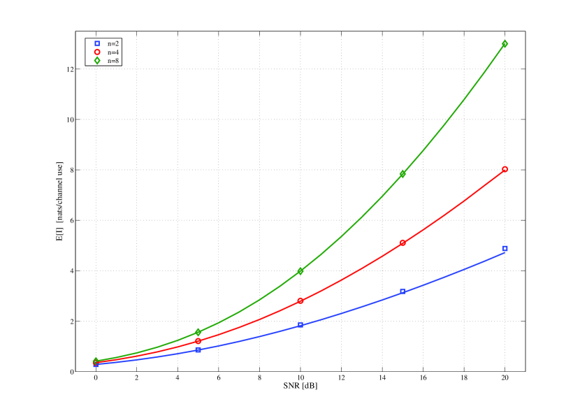
Figure 3: Mutual information versus SNR for $n=n_{\mathrm{s}}=n_{\mathrm{r}}=n_{\mathrm{d}}$ and i.i.d. channel matrix entries – solid lines are analytical approximations, circles, squares and diamonds mark true mutual information as obtained through Monte Carlo simulations.

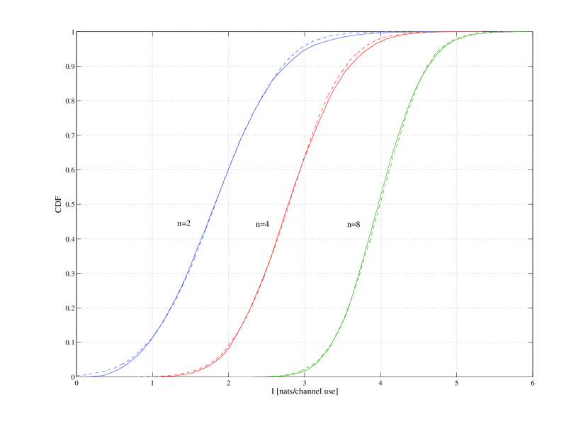
Figure 4: Cumulative distribution function of mutual information for $n=n_{\mathrm{s}}=n_{\mathrm{r}}=n_{\mathrm{d}}$ and i.i.d. channel matrix entries. Dashed lines represent Gaussian distributions with analytically computed mean and variance. The solid lines are the empirical distributions obtained through simulations.

References

- [1] A. L. Moustakas, S. H. Simon, and A. M. Sengupta, “MIMO capacity through correlated channels in the presence of correlated interferers and noise: a (not so) large n analysis,” IEEE Trans. on Inform. Theory, vol. 49, no. 10, p. 2545, Oct. 2003.
- [2] J. Laneman, D. Tse, and G. W. Wornell, “Cooperative diversity in wireless networks: Efficient protocols and outage behavior,” IEEE Trans. Inform. Theory, vol. 50, no. 12, pp. 3062–3080, Dec. 2004.
- [3] J. N. Laneman and G. W. Wornell, “Distributed space-time-coded protocols for exploiting cooperative diversity in wireless networks,” IEEE Trans. Inform. Theory, vol. 49, no. 10, pp. 2415–2425, Oct. 2003.
- [4] A. Sendonaris, E. Erkip, and B. Aazhang, “User cooperation diversity – Part I & Part II,” IEEE Trans. Commun., vol. 51, pp. 1927–1948, Nov. 2003.
- [5] A. Wittneben and B. Rankov, “Impact of cooperative relays on the capacity of rank-deficient MIMO channels,” in Proc. Mobile and Wireless Communications Summit (IST), Aveiro, Portugal, 2003, pp. 421–425.
- [6] G. Kramer, M. Gastpar, and P. Gupta, “Cooperative strategies and capacity theorems for relay networks,” IEEE Trans. Inform. Theory, vol. 51, no. 9, pp. 3037–3063, Sept. 2005.
- [7] M. Gastpar, G. Kramer, and P. Gupta, “The multiple-relay channel: Coding and antenna-clustering capacity,” in Proc. IEEE Int. Symposium on Inf. Theory, Lausanne, Switzerland, June 2002, p. 137.
- [8] A. Host-Madsen, “On the capacity of wireless relaying,” in Proc. 56th IEEE Veh. Tech. Conf., Sept. 2002.
- [9] A. Host-Madsen and J. Zhang, “Capacity bounds and power allocation for wireless relay channels,” IEEE Trans. Inform. Theory, vol. 51, no. 6, pp. 2020–2040, June 2005.
- [10] M. Khojastepour, B. Aazhang, and A. Sabharwal, “On the capacity of ‘cheap’ relay networks,” in Proc. Conference on Information Sciences and Systems (CISS), Princeton, NJ, Apr. 2003.
- [11] R. U. Nabar, O. Oyman, H. Bölcskei, and A. Paulraj, “Capacity scaling laws in MIMO wireless networks,” in Proc. Proc. Allerton Conf. Comm., Contr. and Comp., Oct. 2003, pp. 378–389.
- [12] S. Verdu and S. Shamai (Shitz), “Spectral efficiency of CDMA with random spreading,” IEEE Trans. Inform. Theory, vol. 48, pp. 3117–3128, Dec. 2002.
- [13] P. B. Rapajic and D. Popescu, “Information capacity of a random signature multiple-input multiple-output channel,” IEEE Trans. Commun., vol. 50, no. 9, p. 1245 1248, Aug. 2000.
- [14] X. Mestre, J. R. Fonollosa, and A. Pag s-Zamora, “Capacity of MIMO channels: Asymptotic evaluation under correlated fading,” IEEE Journal on Selected Areas in Communications, vol. 21, no. 5, p. 637 650, June 2003.
- [15] A. Lozano and A. M. Tulino, “Capacity of multiple-transmit multiplereceive antenna architectures,” IEEE Trans. Inform. Theory, vol. 48, no. 3, p. 3117 3128, Dec. 2002.
- [16] T. L. Hochwald B., Marzetta and T. V., “Multiple-antenna channel hardening and its implications for rate feedback and scheduling,” IEEE Trans. Inform. Theory, vol. 50, no. 9, p. 1893 1909, Sep. 2004.
- [17] M. A. Kamath and B. L. Hughes, “The asymptotic capacity of multiple-antenna rayleigh-fading channels,” IEEE Trans. Inform. Theory, vol. 51, no. 12, p. 4325 4333, Dec. 2005.
- [18] V. Morgenshtern and H. Bölcskei, “Random matrix analysis of large relay networks,” in Proc. Allerton Conf. Comm., Contr. and Comp., Sept. 2006.
- [19] S. F. Edwards and P. W. Anderson, “Theory of spin glasses,” J. Phys. F: Metal Phys., vol. 5, no. S2, pp. 965–974, May 1975.
- [20] T. Tanaka, “A statistical-mechanics approach to large-system analysis of CDMA multiuser detectors,” IEEE Trans. Inform. Theory, vol. 48, pp. 2888–2910, Nov. 2002.
- [21] A. M. Sengupta and P. P. Mitra, “Capacity of multivariate channels with multiplicative noise: I. random matrix techniques and large-n expansions for full transfer ma-trices,” LANL arXiv:physics/0010081, Oct. 2000.
- [22] A. M. Tulino and S. Verdu, Random Matrix Theory And Wireless Communications. Now Publishers Inc, 2004.
- [23] R. Müller, “A random matrix model of communication via antenna arrays,” IEEE Trans. Inform. Theory, vol. 48, no. 9, pp. 2495–2506, Sept. 2002.
- [24] ——, “On the asymptotic eigenvalue distribution of concatenated vector-valued fading channels,” IEEE Trans. Inform. Theory, vol. 48, no. 7, pp. 2086–2091, July 2002.
- [25] A. J. Paulraj, R. U. Nabar, and D. Gore, Introduction to Space-Time Wireless Communications. Cambridge University Press, May 2003.
- [26] A. M. Sengupta and P. P. Mitra, “Distributions of singular values for some random matrices,” Phys. Rev. E, vol. 60, no. 3, pp. 3389–3392, 1999.