Statistical Mechanics of On-line Learning when a Moving Teacher Goes around an Unlearnable True Teacher

Abstract

In the framework of on-line learning, a learning machine might move around a teacher due to the differences in structures or output functions between the teacher and the learning machine. In this paper we analyze the generalization performance of a new student supervised by a moving machine. A model composed of a fixed true teacher, a moving teacher, and a student is treated theoretically using statistical mechanics, where the true teacher is a nonmonotonic perceptron and the others are simple perceptrons. Calculating the generalization errors numerically, we show that the generalization errors of a student can temporarily become smaller than that of a moving teacher, even if the student only uses examples from the moving teacher. However, the generalization error of the student eventually becomes the same value with that of the moving teacher. This behavior is qualitatively different from that of a linear model.

1 Introduction

Learning is to infer the underlying rules that dominate data generation using observed data. The observed data are input-output pairs from a teacher and are called examples. Learning can be roughly classified into batch learning and on-line learning [1]. In batch learning, some given examples are used more than once, a paradigm in which a student comes to give correct answers after training if that student has an adequate degree of freedom. However, it is necessary to have a long amount of time and a large memory in which many examples may be stored. On the contrary, examples used once are discarded in on-line learning. In this case, a student cannot give correct answers for all examples used in training. However, there are some merits: for example, a large memory for storing many examples is not necessary and it is possible to follow a time-variant teacher.

Recently, we [6, 7] have analyzed the generalization performance of ensemble learning in a framework of on-line learning using a statistical mechanical method [1, 8]. In that process, the following points were proven subsidiarily: The generalization error does not approach zero when the student is a simple perceptron and the teacher is a committee machine [12] or a non-monotonic perceptron [13]. Therefore, models like these can be called unlearnable cases [9, 10, 11]. The behavior of a student in an unlearnable case depends on the learning rule. That is, the student vector asymptotically converges in one direction using Hebbian learning. On the contrary, the student vector does not converge in one direction but continues moving using perceptron learning or AdaTron learning. In the case of a non-monotonic teacher, the student’s behavior can be expressed by continuing to go around the teacher, keeping a constant direction cosine with the teacher.

Considering the applications of statistical learning theories, investigating the system behaviors of unlearnable cases is significant since real-world problems seem to include many unlearnable cases. In addition, a learning machine may continue going around a teacher in the unlearnable cases as mentioned above. Here, let us consider a new student that is supervised by a moving learning machine. That is, we consider a student that uses the input-output pairs of a moving teacher as training examples, and we investigate the generalization performance of a student for a true teacher. Here, the true teacher is fixed. Note that the examples used by the student are only from the moving teacher, and the student cannot directly observe the outputs of the true teacher. In a real human society, a teacher that can be observed by a student does not always present the correct answer; in many cases, the teacher is learning and continues to vary. Therefore, analyzing such a model is interesting for considering the analogies between statistical learning theories and a real society.

A model in which a true teacher, a moving teacher, and a student are all linear perceptrons [6] with noises was already solved analytically[14]. It was proved that a student’s generalization errors can be smaller than that of the moving teacher in the linear case even though the student uses only the examples of the moving teacher. However, linear perceptrons are somewhat special as neural networks or learning machines. Nonlinear perceptrons are more common than linear ones. Therefore, in this paper we treat a model in which a true teacher, a moving teacher, and a student are all nonlinear perceptrons. We calculate the order parameters and the generalization errors in the case of a true teacher as nonmonotonic while the others are simple perceptrons theoretically using a statistical mechanical method in the framework of on-line learning. As a result, it is proved that a student’s generalization errors can be smaller than that of the moving teacher. That means the student can be cleverer than the moving teacher even though the student uses only the examples from the moving teacher. Although these behaviors are analogous to those of a linear model, the generalization error of the student eventually becomes the same value as that of the moving teacher in the nonlinear model.

2 Model

Three nonlinear perceptrons are treated in this paper: a true teacher, a moving teacher and a student. Their connection weights are $\mbox{\boldmath$A$},\mbox{\boldmath$B$}$, and $J$, respectively. For simplicity, the connection weights of the true teacher, that of the moving teacher and that of the student are simply called the true teacher, the moving teacher, and the student, respectively. The true teacher $\mbox{\boldmath$A$}=(A_{1},\ldots,A_{N})$, the moving teacher $\mbox{\boldmath$B$}=(B_{1},\ldots,B_{N})$, the student $\mbox{\boldmath$J$}=(J_{1},\ldots,J_{N})$, and input $\mbox{\boldmath$x$}=(x_{1},\ldots,x_{N})$ are $N$-dimensional vectors. Each component $A_{i}$ of $A$ is drawn from ${\cal N}(0,1)$ independently and fixed, where ${\cal N}(0,1)$ denotes the Gaussian distribution with a mean of zero and a variance of unity. Each of the components $B_{i}^{0},J_{i}^{0}$ of the initial values of $\mbox{\boldmath$B$},\mbox{\boldmath$J$}$ are drawn from ${\cal N}(0,1)$ independently. Each component $x_{i}$ of $x$ is drawn from ${\cal N}(0,1/N)$ independently. Thus,

$$\left\langle A_{i}\right\rangle =0, \left\langle(A_{i})^{2}\right\rangle =1,$$ (1)

$$\left\langle B_{i}^{0}\right\rangle =0, \left\langle(B_{i}^{0})^{2}\right\rangle =1,$$ (2)

$$\left\langle J_{i}^{0}\right\rangle =0, \left\langle(J_{i}^{0})^{2}\right\rangle =1,$$ (3)

$$\left\langle x_{i}\right\rangle =0, \left\langle(x_{i})^{2}\right\rangle =\frac{1}{N},$$ (4)

where $\langle\cdot\rangle$ denotes a mean.

In this paper, the thermodynamic limit $N\rightarrow\infty$ is also treated. Therefore,

$$\|\mbox{\boldmath$A$}\|=\sqrt{N},\ \ \|\mbox{\boldmath$B$}^{0}\|=\sqrt{N},\ \ \|\mbox{\boldmath$J$}^{0}\|=\sqrt{N},\ \ \|\mbox{\boldmath$x$}\|=1,$$ (5)

where $\|\cdot\|$ denotes a vector norm. Generally, norms $\|\mbox{\boldmath$B$}\|$ and $\|\mbox{\boldmath$J$}\|$ of the moving teacher and the student change as the time step proceeds. Therefore, the ratios $l_{B}$ and $l_{J}$ of the norms to $\sqrt{N}$ are introduced and are called the length of the moving teacher and the length of the student. That is, $\|\mbox{\boldmath$B$}\|=l_{B}\sqrt{N}$ C $\|\mbox{\boldmath$J$}\|=l_{J}\sqrt{N}$.

The internal potentials $y$ of the true teacher, $vl_{B}$ of the moving teacher, and $ul_{J}$ of the student are

$$y = \mbox{\boldmath$A$}\cdot\mbox{\boldmath$x$},$$ (6)

$$vl_{B} = \mbox{\boldmath$B$}\cdot\mbox{\boldmath$x$},$$ (7)

$$ul_{J} = \mbox{\boldmath$J$}\cdot\mbox{\boldmath$x$},$$ (8)

where $y$, $v$, and $u$ obey the Gaussian distributions with means of zero and variances of unity.

The output of the true teacher, which has a nonmonotonic output function, is

$$d=\mbox{sgn}((y-a)y(y+a)),$$ (9)

where $a$ is a fixed threshold of the nonmonotonic function. The outputs of the moving teacher and the student, which are simple perceptrons, are $\mbox{sgn}(vl_{B})$ and $\mbox{sgn}(ul_{J})$, respectively. Here, $\mbox{sgn}(\cdot)$ is a sign function defined as

$$\mbox{sgn}(z) = \left\{\begin{array}[]{ll}+1,&z\geq 0,\\ -1,&z<0.\end{array}\right.$$ (12)

In the model treated in this paper, the moving teacher $B$ is updated using an input $x$ and an output of the true teacher $A$ for the input $x$. The student $J$ is updated using an input $x$ and an output of the moving teacher $B$ for the input $x$. The moving teacher is considered to use perceptron learning. That is,

$$\mbox{\boldmath$B$}^{m+1} = \mbox{\boldmath$B$}^{m}+\eta_{B}\Theta(-v^{m}d^{m})d^{m}\mbox{\boldmath$x$}^{m}$$ (13)

$$= \mbox{\boldmath$B$}^{m}+\eta_{B}\Theta(-v^{m}(y^{m}-a)y^{m}(y^{m}+a))\mbox{sgn}((y^{m}-a)y^{m}(y^{m}+a))\mbox{\boldmath$x$}^{m},$$ (14)

where $\eta_{B}$ denotes the learning rate of the moving teacher and is a constant number. Furthermore, $m$ denotes the time step, and $\Theta(\cdot)$ denotes the step function defined as

$$\Theta(z) = \left\{\begin{array}[]{ll}+1,&z\geq 0,\\ 0,&z<0.\end{array}\right.$$ (17)

The student is also considered to use perceptron learning. That is,

$$\mbox{\boldmath$J$}^{m+1} = \mbox{\boldmath$J$}^{m}+\eta_{J}\Theta(-u^{m}v^{m})\mbox{sgn}(v^{m})\mbox{\boldmath$x$}^{m},$$ (18)

where $\eta_{J}$ denotes the student’s learning rate and is a constant number. Generalizing the learning rules, Eqs. (14) and (18) can be expressed as

$$\mbox{\boldmath$B$}^{m+1} = \mbox{\boldmath$B$}^{m}+g^{m}\mbox{\boldmath$x$}^{m},$$ (19)

$$\mbox{\boldmath$J$}^{m+1} = \mbox{\boldmath$J$}^{m}+f^{m}\mbox{\boldmath$x$}^{m},$$ (20)

respectively. Here, $g$ and $f$ are update functions of the moving teacher and the student, respectively.

3 Theory

3.1 Generalization Error

A goal of a statistical learning theory is to theoretically obtain generalization errors. We use

$$\epsilon_{B}^{m} = \Theta\left(-d^{m}\mbox{sgn}(v^{m}l_{B}^{m})\right)$$ (21)

$$= \Theta\left(-(y^{m}-a)y^{m}(y^{m}+a)v^{m}\right)$$ (22)

and

$$\epsilon_{J}^{m} = \Theta\left(-d^{m}\mbox{sgn}(u^{m}l_{J}^{m})\right)$$ (23)

$$= \Theta\left(-(y^{m}-a)y^{m}(y^{m}+a)u^{m}\right)$$ (24)

as errors of the moving teacher and student, respectively. The superscripts $m$, which represent the time steps, are omitted for simplicity. We define a generalization error as a mean of error over the distribution $p(\mbox{\boldmath$x$})$ of inputs $x$. The error $\epsilon_{B}$ of the moving teacher and the error $\epsilon_{J}$ of the student can be expressed as $\epsilon_{B}(y,v)$ and $\epsilon_{J}(y,u)$ using $y,v$, and $u$, Therefore, the generalization error $\epsilon_{gB}$ of the moving teacher and the generalization error $\epsilon_{gJ}$ of the student can be calculated using the distributions $p(y,v)$ and $p(y,u)$ as follows:

$$\epsilon_{gB} = \langle\epsilon_{B}\rangle_{\bm{x}}$$ (25)

$$= \int d\mbox{\boldmath$x$}p(\mbox{\boldmath$x$})\epsilon_{B}$$ (26)

$$= \int dydvp(y,v)\epsilon_{B}(y,v),$$ (27)

$$\epsilon_{gJ} = \langle\epsilon_{J}\rangle_{\bm{x}}$$ (28)

$$= \int d\mbox{\boldmath$x$}p(\mbox{\boldmath$x$})\epsilon_{J}$$ (29)

$$= \int dydup(y,u)\epsilon_{J}(y,u).$$ (30)

Since $y,v$ and $u$ are calculated using $\mbox{\boldmath$A$},\mbox{\boldmath$B$},\mbox{\boldmath$J$}$, and the independent input $x$, $p(y,v,u)$ is the multiple Gaussian distribution with means of zero and the covariance matrix $\Sigma$

$$\Sigma = \left(\begin{array}[]{ccc}1&R_{B}&R_{J}\\ R_{B}&1&R_{BJ}\\ R_{J}&R_{BJ}&1\end{array}\right).$$ (34)

Here, $R_{B}$ is the direction cosine between $A$ and $B$. $R_{J}$ is the direction cosine between $A$ and $J$. $R_{BJ}$ is the direction cosine between $B$ and $J$. Thus,

$$R_{B} = \frac{\mbox{\boldmath$A$}\cdot\mbox{\boldmath$B$}}{\|\mbox{\boldmath$A$}\|\|\mbox{\boldmath$B$}\|},$$ (35)

$$R_{J} = \frac{\mbox{\boldmath$A$}\cdot\mbox{\boldmath$J$}}{\|\mbox{\boldmath$A$}\|\|\mbox{\boldmath$J$}\|},$$ (36)

$$R_{BJ} = \frac{\mbox{\boldmath$B$}\cdot\mbox{\boldmath$J$}}{\|\mbox{\boldmath$B$}\|\|\mbox{\boldmath$J$}\|}.$$ (37)

Equations (27) and (30) can be calculated by excuting the Gaussian integrations using these direction cosines as follows[9, 10, 11]:

$$\epsilon_{gB} = \int_{0}^{a}DyH\left(\frac{-yR_{B}}{\sqrt{1-R_{B}^{2}}}\right)+\int_{\infty}^{-a}DyH\left(\frac{-yR_{B}}{\sqrt{1-R_{B}^{2}}}\right),$$ (38)

$$\epsilon_{gJ} = \int_{0}^{a}DyH\left(\frac{-yR_{J}}{\sqrt{1-R_{J}^{2}}}\right)+\int_{\infty}^{-a}DyH\left(\frac{-yR_{J}}{\sqrt{1-R_{J}^{2}}}\right),$$ (39)

where

$$H(u)\equiv\int_{u}^{\infty}Dy,\ \ \ Dy\equiv\frac{dy}{\sqrt{2\pi}}\exp\left(-\frac{y^{2}}{2}\right).$$ (40)

The relationship among the true teacher $A$, the moving teacher $B$, and the student $J$ is shown in Fig. 1.

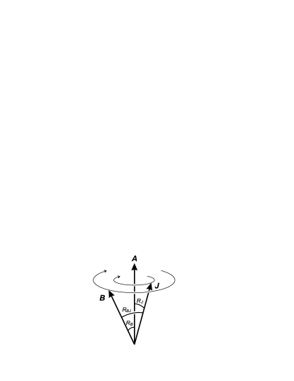
Figure 1: True teacher $A$, moving teacher $B$, and student $J$. $R_{B},R_{J}$, and $R_{BJ}$ are direction cosines.

3.2 Differential equations of order parameters

Since we treat the thermodynamic limit $N\rightarrow\infty$ in this paper, $O(N)$ updates of Eqs. (14) and (18) are necessary for the order parameters to change $O(1)$. Therefore, we denote time steps $m$ normalized by the dimension $N$ as a continuous time $t=m/N$. We use $t$ as a subscript for the learning process.

The generalization errors $\epsilon_{gB}$ and $\epsilon_{gJ}$ can be calculated if all the order parameters $R_{B}$, $R_{J}$ and $R_{BJ}$ are known. Therefore, simultaneous differential equations in deterministic forms [8] have been obtained that describe the dynamical behaviors of order parameters based on self-averaging in the thermodynamic limits as follows[14]:

$$\frac{dl_{B}}{dt} =\langle gv\rangle+\frac{\langle g^{2}\rangle}{2l_{B}},$$ (41)

$$\frac{dl_{J}}{dt} =\langle fu\rangle+\frac{\langle f^{2}\rangle}{2l_{J}},$$ (42)

$$\frac{dR_{BJ}}{dt} =-R_{BJ}\left(\frac{1}{l_{J}}\frac{dl_{J}}{dt}+\frac{1}{l_{B}}\frac{dl_{B}}{dt}\right)+\frac{1}{l_{B}}\langle gu\rangle+\frac{1}{l_{J}}\langle fv\rangle+\frac{1}{l_{B}l_{J}}\langle gf\rangle,$$ (43)

$$\frac{dR_{J}}{dt} =\frac{1}{l_{J}}\left(-R_{J}\frac{dl_{J}}{dt}+\langle fy\rangle\right),$$ (44)

$$\frac{dR_{B}}{dt} =\frac{\langle gy\rangle-\langle gv\rangle R_{B}}{l_{B}}-\frac{R_{B}}{2l_{B}^{2}}\langle gy\rangle.$$ (45)

As mentioned above, $y$, $v$, and $u$ obey the triple Gaussian distribution with means of zero and the covariance matrix of Eq. (34). Using this, we can calculate the nine sample averages that appear in Eqs. (41)–(45) as follows:

$$\langle gv\rangle =\frac{\eta_{B}}{\sqrt{2\pi}}\left(R_{B}\left(2\exp\left(-\frac{a^{2}}{2}\right)-1\right)-1\right),$$ (46)

$$\langle g^{2}\rangle =2{\eta}_{B}^{2}\left(\int_{0}^{a}D_{y}H\left(\frac{-yR_{B}}{\sqrt{1-R_{B}^{2}}}\right)+\int_{\infty}^{-a}D_{y}H\left(\frac{-yR_{B}}{\sqrt{1-R_{B}^{2}}}\right)\right),$$ (47)

$$\langle fu\rangle ={\eta}_{J}\frac{R_{BJ}-1}{\sqrt{2\pi}},$$ (48)

$$\langle f^{2}\rangle =\frac{{\eta}_{J}^{2}}{\pi}{\tan}^{-1}\frac{\sqrt{1-R_{BJ}^{2}}}{R_{BJ}},$$ (49)

$$\langle gu\rangle =\frac{\eta_{B}}{\sqrt{2\pi}}\left(R_{J}\left(2\exp\left(-\frac{a^{2}}{2}\right)-1\right)-R_{BJ}\right),$$ (50)

$$\langle fv\rangle ={\eta}_{J}\frac{1-R_{BJ}}{\sqrt{2\pi}},$$ (51)

$$\langle gf\rangle =-2{\eta}_{B}{\eta}_{J}\left(\int_{0}^{a}D_{y}+\int_{-\infty}^{a}D_{y}\right)\int_{-\frac{yR_{B}}{\sqrt{1-R_{B}^{2}}}}^{\infty}DvH\left(-\frac{yR_{J}\sqrt{1-R_{B}^{2}}+v(R_{B}R_{J}-R_{BJ})}{\sqrt{1+2R_{B}R_{J}R_{BJ}-R_{B}^{2}-R_{J}^{2}-R_{BJ}^{2}}}\right),$$ (52)

$$\langle fy\rangle ={\eta}_{J}\frac{R_{B}-R_{J}}{\sqrt{2\pi}},$$ (53)

$$\langle gy\rangle =\frac{{\eta}_{B}}{\sqrt{2\pi}}\left(2\exp\left(-\frac{a^{2}}{2}\right)-1-R_{B}\right).$$ (54)

4 Results and discussion

Figures 2–5 illustrate the dynamical behaviors of the generalization errors and the order parameters. The threshold $a$ of the true teacher is $0.5$ and the learning rate $\eta_{B}$ of the moving teacher is $0.1$. In these figures, the curves represent the theoretical results and the symbols represent the simulation results, where $N=10^{4}$. In theoretical calculations, the simultaneous differential equations have been solved numerically using the sample averages in Eqs. (41)–(45) also obtained numerically. The generalization errors $\epsilon_{gB}$ and $\epsilon_{gJ}$ are calculated by executing integrations in Eqs. (38) and (39) numerically using the obtained $R_{B},R_{J}$, and $R_{BJ}$. In the computer simulations, the generalization errors have been measured through tests using $10^{5}$ random inputs at each time step. In these figures, the theoretical results and the computer simulations closely agree with each other.

Figure 2 shows that the student’s generalization error $\epsilon_{gJ}$ is always larger than $\epsilon_{gB}$ of the moving teacher when the student’s learning rate $\eta_{J}$ is relatively large, for example $\eta_{J}=1.0$. In that case, $\epsilon_{gJ}$ approaches $\epsilon_{gB}$ asymptotically. On the other hand, $\epsilon_{gJ}$ temporarily becomes smaller than $\epsilon_{gB}$ when the learning rate $\eta_{J}$ is relatively small, for example $\eta_{J}=0.2,0.05$ or $0.01$. This is an interesting phenomenon since the student can temporarily become cleverer than the moving teacher even though the student uses only the examples from the moving teacher. This is the same as the linear case[14] whereby $\epsilon_{gJ}$ can become smaller than $\epsilon_{gB}$. In the linear case[14], a small $\epsilon_{gJ}$ is maintained after $\epsilon_{gJ}$ becomes smaller than $\epsilon_{gB}$. However, $\epsilon_{gJ}$ returns to the same value as $\epsilon_{gB}$ in the nonlinear case treated in this paper. This behavior is interesting since it is qualitatively different from the linear case. In addition, the overshot of $\epsilon_{gJ}$ occurs only once when $\eta_{J}=0.2$. On the other hand, $\epsilon_{gJ}$ swings three times when $\eta_{J}=0.05,0.01$.

Figure 3 shows that $R_{J}$ temporarily becomes larger than $R_{B}$ when $\eta_{J}$ is small. This means that $J$ comes closer to $A$ than $B$. Although the overshot of $R_{J}$ occurs only once, $\epsilon_{gJ}$ swings three times when $\eta_{J}=0.05,0.01$. The reason for this difference can be understood as follows. In the case of a nonmonotonic teacher, the relationship between the generalization error $\epsilon_{g}$ and the direction cosine $R$ is Eq. (38) or (39)[9, 10, 11]. In the case of $a<\sqrt{2\ln 2}=1.18$, $\epsilon_{g}$ is not a monotonic function of $R$ and takes a minimum value when $R=\sqrt{(2\ln 2-a^{2})/(2\ln 2)}$. Since $a=0.5$ is treated in this section, $\epsilon_{g}$ takes a minimum value when $R=0.905$. The theoretical curves of $\eta_{J}=0.05,0.01$ in Fig. 3 indicate that $R$ agrees with $0.905$ twice. This phenomenon corresponds to the two local minima in Fig. 2. On the other hand, $R$ does not reach $0.905$ when $\eta_{J}=0.2$. Therefore, the number of the minimum of $\epsilon_{g}$ is also only one.

Figure 3 shows that the maximum value of $R_{J}$ is unity when $\eta_{J}=0.01$. This is also a very interesting phenomenon since the direction cosine between a teacher and a student does not reach unity when the student learns the nonmonotonic teacher using perceptron learning[11].

In addition, $R_{B}$ and $R_{J}$ agree with each other after enough time steps. However, the moving teacher and the student do not coincide with each other. That is, $R_{BJ}$ is smaller than unity as shown in Fig. 4.

Figure 2: Dynamical behaviors of $\epsilon_{gB}$ and $\epsilon_{gJ}$. Conditions are $a=0.5$ and $\eta_{B}=0.1$. Curves represent theoretical results and symbols represent simulation results, where $N=10^{4}$.

Figure 3: Dynamical behaviors of $R_{B}$ and $R_{J}$. Conditions are $a=0.5$ and $\eta_{B}=0.1$. Curves represent theoretical results and symbols represent simulation results, where $N=10^{4}$.

Figure 4: Dynamical behaviors of $R_{BJ}$. Conditions are $a=0.5$ and $\eta_{B}=0.1$. Curves represent theoretical results and symbols represent simulation results, where $N=10^{4}$.

Figure 5: Dynamical behaviors of $l_{B}$ and $l_{J}$. Conditions are $a=0.5$ and $\eta_{B}=0.1$. Curves represent theoretical results and symbols represent simulation results, where $N=10^{4}$.

5 Conclusion

In the framework of on-line learning, a learning machine might move around a teacher due to the differences in structures or output functions between the teacher and the learning machine. In this paper we analyzed the generalization performance of a new student supervised by a moving machine. A model composed of a fixed true teacher, a moving teacher, and a student was treated theoretically using statistical mechanics, where the true teacher is a nonmonotonic perceptron and the others are simple perceptrons. Calculating the generalization errors numerically, we have shown that a student’s the generalization error can temporarily become smaller than that of a moving teacher, even if the student only uses examples from the moving teacher. However, the student’s generalization error eventually becomes the same value as that of the moving teacher. This behavior is qualitatively different from that of a linear model.

References

• [1] D. Saad, (ed.): On-line Learning in Neural Networks (Cambridge University Press, Cambridge, 1998).
• [2] Y. Freund, and R. E. Schapire: Journal of Japanese Society for Artificial Intelligence, 14 (1999) 771 [in Japanese, translation by N. Abe].
• [3] http://www.boosting.org/
• [4] A. Krogh, and P. Sollich: Phys. Rev. E 55 (1997) 811.
• [5] R. Urbanczik: Phys. Rev. E 62 (2000) 1448.
• [6] K. Hara and M. Okada: J. Phys. Soc. Jpn. 74 (2005) 2966.
• [7] S. Miyoshi, K. Hara and M. Okada: Phys. Rev. E 71 (2005) 036116.
• [8] H. Nishimori: Statistical Physics of Spin Glasses and Information Processing: An Introduction (Oxford University Press, Oxford, 2001).
• [9] J. I. Inoue and H. Nishimori: Phys. Rev. E 55 (1997) 4544.
• [10] J. I. Inoue, H. Nishimori and Y. Kabashima: cond-mat/9708096 (1997).
• [11] J. I. Inoue, H. Nishimori and Y. Kabashima: J. Phys. A: Math. Gen. 30 (1997) 3795.
• [12] S. Miyoshi, K. Hara and M. Okada: Proc. The Seventh Workshop on Information-Based Induction Sciences (2004) 178 [in Japanese].
• [13] S. Miyoshi, K. Hara and M. Okada: IEICE Technical Report, NC2004-214 (2005) 123 [in Japanese].
• [14] S. Miyoshi and M. Okada: Journal of Physical Society of Japan, Vol.75, No.2, 024003, Feb. 2006.