Towards Parallel Computing on the Internet: Applications, Architectures, Models and Programming Tools

Abstract

The development of Internet wide resources for general purpose parallel computing poses the challenging task of matching computation and communication complexity. A number of parallel computing models exist that address this for traditional parallel architectures, and there are a number of emerging models that attempt to do this for large scale Internet-based systems like computational grids. In this survey we cover the three fundamental aspects – application, architecture and model, and we show how they have been developed over the last decade. We also cover programming tools that are currently being used for parallel programming in computational grids. The trend in conventional computational models are to put emphasis on efficient communication between participating nodes by adapting different types of communication to network conditions. Effects of dynamism and uncertainties that arise in large scale systems are evidently important to understand and yet there is currently little work that addresses this from a parallel computing perspective.

1 Introduction

The field of High Performance Computing (HPC) has evolved to include a variety of very complex architectures, computing models and problem solving environments. HPC architectures consist of Massively Parallel Processors (MPPs), clusters and constellation architectures and they typically use hundreds to hundreds of thousands of CPUs. Some application problems involve large real time data that must be processed as soon as possible, while others involve a high degree of computational complexity. Computing models on the other hand, provide a bridge between hardware and software to assist application developers in designing and writing parallel applications that efficiently utilize the available parallel architecture. Problem solving environments provide comprehensive computational facilities for programmers to develop parallel applications on these platforms. These environments usually consists of programming tools, utilities, libraries, debuggers, profilers, etc.

The extent to which a system can be called a HPC architecture is relatively ambiguous and dynamic, because the contemporary HPC architecture and notion of HPC can be liberally extended to cover collections of resources that are combined to solve a single problem. These definitions lead us to consider computational grids [40] as (commodity) supercomputers and indeed computational grids are being used to solve problems that were and still are sometimes solved by the classical HPC architectures. In general, it is clear that problems are migrating from classical HPC architectures towards the contemporary computational grid (or at least that the use of the Internet is becoming prevalent in order to tie more computing resources together), either explicitly by direct programming efforts or implicitly through virtualization. Some problems are harder than others to migrate and this survey covers the approaches that have and are being used to overcome the associated difficulties.

Developing applications for HPC is not comparable to developing applications for a single processor mainly because of the complexity involved in the HPC architectures. The challenge that this survey addresses is how the application developer can understand the differences in complexity between the problem and communication imposed by the architecture. By surveying the past and present computational models and in particular those that are associated with computational grids we provide a resource for future parallel programmers to better understand the ways in which the computational grid architecture affects their programs. A model allows the determination of computational and communication complexities associated with a given problem, as expressed by the hardware. It plays an important role to reflect the salient computing characteristics of a particular architecture to develop fast and efficient algorithms and provides information on the performance of an application.

When developing application software for HPC, parallel application developers must emphasize both extreme ends of the architecture, namely the memory hierarchy and the inter-processor communication. This is due to the cost associated in accessing large data sets. Furthermore, the rate of data access is not as fast as the rate of computation performed by processors due to bandwidth limitation for both the inter-processor and processor-memory data transfer. All of the emerging models therefore consider the data movement costs in a system under consideration, as accurately as possible. It is also important to note that a model may provide good representation of an architecture, but to gauge an application’s performance it is necessary to take into consideration how efficiently the application can be implemented (efficiency of coding).

Relationships between HPC architectures, problem solving tools, and applications requiring HPC are shown in Fig. 1. The overlapping region A, depicts the computational performance of a parallel program, region B shows the use of problem solving tools and algorithms to solve the problem without considering the parallel architecture, region C represents performance tuning parameters with information from parallel architecture, and region D represents algorithms and the requirements for solving the problem in a reasonable amount of time. HPC architectures and grand challenge problems decide which type of model should be used and in turn the model decides parameters to be used in the programming language.

Figure 1: The relationship between HPC architectures, problem solving tools and applications requiring HPC.

Overlapping Region.	Description.
A	Computational model providing information on performance of parallel programs.
B	Algorithm parameters (e.g data size, communication type, computational complexity, etc.) and problem solving tools.
C	Performance tuning parameters (e.g. number of processors, latency, bandwidth, shared/distributed memory, etc.).
D	Requirements for solving problem in reasonable amount of time (e.g. storage, memory & computational capacity, number of processors and algorithms).

Table 1: Explanation for the overlapping region in Fig. 1.

1.1 Objective

The main objective of this paper is to show the importance of an accurate computational model in solving large scale application on HPC architectures. We begin by looking at some of the applications that require HPC, the characteristics of these applications such as memory requirements, computational requirements, storage space, communication and computational complexity, and algorithms required to solve this problem. Later, we look at the characteristics of architectures that have evolved to attempt to solve these application as fast as possible. Here we list some of the important characteristics of these architectures. The motivation for new HPC architectures are the challenges introduced by the large scale problems, while the motivation for computational models are to efficiently solve the problems on the available architecture. Some architectures are more suitable for certain types and sizes of problems, and it is important to have an idea beforehand on the suitability of the architecture before the problem is solved on it. This is where the computational model will play its role as a bridge between them. Hence, we study some of the more popular parallel computational models that have been used in the past and also look at some of the conventional computational models. It becomes clear that the new models are moving towards the direction of assisting adaptation of parallel computing softwares to the dynamic behavior of the architecture.

1.2 Organization

We divide this paper into six main sections. In Section  2, we look at different applications that require the use of HPC architectures. We list some significant characteristics of these applications that highlights the configuration requirement for HPC. Next, in Section  3, we briefly look at recent HPC architectures. Here we list some of the important properties of these architectures. This is important to measure how the parallel computing model has evolved to better reflect HPC architectures. Section  4, looks at traditional parallel computing models and conventional parallel models used to design parallel algorithm and predict performance of HPC architectures. In this section, we investigate factors considered by different parallel models that have been developed and look at how the development in architectures have influenced the models. We also discuss some parallel computing models that are developed for Grid environment. Section  5, discusses some of the popular parallel programming libraries used by HPC communities for both traditional supercomputers and also the Grid. Section  6, concludes the paper and provides suggestion on attributes that should be considered for parallel computing model on Grid environment.

2 Applications challenges

In this section, we describe the ever increasing need for HPC facilities and we give insight into the computational complexities and other demands of a number of applications in the field of computational science; which is useful for identifying the required HPC facilities and computational models.

Many fields in science and engineering have computationally intensive problems that are intractable without the use of HPC. Most of these problems come under the category of computational sciences. Problems such as climate modeling (which consists of atmosphere model, ocean model, hurricane model, hydrological model and sea-ice model), plasma physics (to produce safe, clean and cost-effective energy from nuclear fusion), engineering design (of aircraft, ships, and vehicles), bio-informatics and computational biology, geophysical exploration and geoscience, astrophysics, material science and nanotechnology, defense (cracking cryptography code), computational fluid dynamics, and computational physics are computationally demanding. The characteristics of these applications listed in Table  LABEL:app_char are:

Memory requirement

The size of main memory required to store data for computation. This measurement is important for selection of suitable computing resources. Resources with memory less than this threshold will deteriorate the application performance as more time will be required to access data from secondary storage.

Computational requirement

The amount of Floating Point Operations per Second (FLOPS) required to undertake the complexity of the problem in a “reasonable amount of time” as some application involves real-time data. This measure depends on several factors such as abstraction of the problem and the size of computation.

Storage

The minimum amount of storage space required by the application to store simulation results for visualization purposes or to store sufficient amount of data to be used in computation for “reasonable amount of accuracy”. This value will be useful to chose resources that meet the requirement and avoid loss of information.

Communication complexity

Is the amount of information that needs to be communicated between computing nodes to successfully complete a computation. This provides information on the communication needs of an algorithm for executing across multiple computing nodes. It is in particular important for the purpose of selecting optimal number of resources to use for a particular problem size.

Computational complexity

This gives information on how the complexity of an algorithm grows as the size of the problem increases. This information is critical for choosing appropriate computing resources.

Algorithms

Different types of algorithms that can be used to solve a particular problem.

A typical problem of computational science involves finding the solution to models of real world phenomenon. Many of these models use Partial Differential Equations (PDEs) and are approximated using discretized equations. For better approximation, higher resolution must be used and this demands more computational power. All of these grand challenge problems are difficult to be solve efficiently with better accuracy due to a number of reasons: 1) Limitation in capability of hardwares, 2) Algorithms used to solve the problems and 3) Tools that are available for a programmer to solve these problems and analyze the results. The term “Grand Challenge” used in previous statement was coined by Nobel Laureate Kenneth G. Wilson, who also articulated the current concept of “computational science” as a third way of doing science [50]. The Grand Challenge problems have the following properties in common: 1) They are questions to which many scientists and engineers would like to know answers; 2) They are difficult and it is not known how to do them right now; 3) It may be done using computers but the current computers are not fast enough. [50]

Basic algorithms and numerical algorithms play important role in many computationally intensive scientific applications. Some of these grand challenge applications and algorithms that are used to solve them using HPC are depicted in Fig. 2 . It is interesting to observe that all these applications depend on some of the most fundamental algorithms. Many highly tuned parallel computational libraries and computational kernels are available for these algorithms to be used on dedicated computing platforms. However, they are not proven to be as efficient on computing resources distributed across the WAN.

Table 2: Characteristics of Grand Challenge applications.

Applications	Memory requirement	Computational requirement	Storage	Communication complexity	Computational complexity
Climate Modeling: Atmosphere model resolution of $75km$ and ocean model resolution of $10km$.	$>1$TB depending on the resolution of model.	$100$–$150$ TFLOP/s for high resolution and highly complex model	$>23$TB for a single century simulation.	FFT–$\mathop{\mathrm{O}}\bigl{(}P^{2}\bigr{)}$ where $P$ is the No. of processors.	$\mathop{\mathrm{O}}\bigl{(}N^{2}\bigr{)}$ with $N$–Size of resolution.
Algorithms: FFT, Finite Difference, Finite element method.
Bioinformatics and Computational biology.	$>$ Several hundred MB/processor.	$\approx 100$ TFLOP/s–few PFLOP/s.	$>1$PB.	$\mathop{\mathrm{O}}\bigl{(}P\bigr{)}$–$\mathop{\mathrm{O}}\bigl{(}P^{2}\bigr{)}$ where $P$ is the No. of processors.	$\mathop{\mathrm{O}}\bigl{(}N^{2}\bigr{)}$–$\mathop{\mathrm{O}}\bigl{(}N^{3}\bigr{)}$ where $N$ is the No. of atoms.
Algorithms: Complex Combinatorial, Graph Theoretic, Differential Equation Solver.
Astrophysics simulations.	$>10$TB.	$\approx 100$TFLOP/s–$10$PFLOP/s.	$>1$PB.	FMM:$\mathop{\mathrm{O}}\bigl{(}loglog(P)\bigr{)}$ and $\mathop{\mathrm{O}}\bigl{(}log(P)\bigr{)}$ for balanced and exponential distribution respectively, FFT–$\mathop{\mathrm{O}}\bigl{(}P^{2}\bigr{)}$ where $P$ is the No. of processors.	$\mathop{\mathrm{O}}\bigl{(}N^{10}\bigr{)}$–$\mathop{\mathrm{O}}\bigl{(}N^{15}\bigr{)}$ where $N$ is the size of the problem.
Algorithms: Fast Multipole Method (FMM), Multi-Scale Dense Linear Algebra, Parallel $3$D FFTs, Spherical Transforms,
Particle methods and adaptive mesh refinement.
Computational material science and Nanoscience.		several PFLOP/s		FFT–$\mathop{\mathrm{O}}\bigl{(}P^{2}\bigr{)}$ where $P$ is the No. of processors.	$\mathop{\mathrm{O}}\bigl{(}N^{3}\bigr{)}$–$\mathop{\mathrm{O}}\bigl{(}N^{7}\bigr{)}$ with $N$ as No. of atoms in a molecule.
Algorithms: Quantum Molecular Dynamics (QMD), Quantum Monte Carlo (QMC), Dense Linear Algebra,
Parallel $3$D FFT, Iterative Eigen Solvers.
Computational Fluid Dynamics (CFD).	$>400$GB for double precision arithmetic.	$1$ PFLOP/s–few PFLOP/s.	$1$TB.	$\mathop{\mathrm{O}}\bigl{(}P\bigr{)}$–$\mathop{\mathrm{O}}\bigl{(}P^{2}\bigr{)}$ where $P$ is the No. of processors	$\mathop{\mathrm{O}}\bigl{(}Nlog(N)\bigr{)}$–$\mathop{\mathrm{O}}\bigl{(}N^{2}\bigr{)}$ where $N$ is the size of the problem.
Algorithms: Finite Difference, Finite Element, Finite Volume, Pseudospectral and Spectral methods.
Computational Physics.
Plasma science.	$>50$TB	$100$TFLOPs–few PFLOP/s.	$>27$PB	$\mathop{\mathrm{O}}\bigl{(}P\bigr{)}$–$\mathop{\mathrm{O}}\bigl{(}P^{2}\bigr{)}$ where $P$ is the No. of processors.	$\mathop{\mathrm{O}}\bigl{(}N^{10}\bigr{)}$.
Algorithms: Gyrokinetic (GK), Gyro-Landau-fluid (GLF), Nonlinear Solvers, Adaptive Mesh Refinement,
Dense Linear Algebra and Particle Methods.
Particle Accelerator Simulation.
Electron cooling.	$>5$GB.	$\approx 10^{6}$–$10^{7}$ TFLOPS per run.	$>2$TB	$\mathop{\mathrm{O}}\bigl{(}P\bigr{)}$–$\mathop{\mathrm{O}}\bigl{(}P^{2}\bigr{)}$, where $P$ is the No. of processors.	$\mathop{\mathrm{O}}\bigl{(}NlogN\bigr{)}$–$\mathop{\mathrm{O}}\bigl{(}N^{2}\bigr{)}$
Beam heating.	$>1$TB.	$\approx 10^{3}$–$10^{4}$ TFLOPS per run.	$>2$TB	$\mathop{\mathrm{O}}\bigl{(}P\bigr{)}$-$\mathop{\mathrm{O}}\bigl{(}P^{2}\bigr{)}$, with $P$ is the No. of processors.	$\mathop{\mathrm{O}}\bigl{(}NlogN\bigr{)}$–$\mathop{\mathrm{O}}\bigl{(}N^{2}\bigr{)}$
Algorithms: Fast Fourier Transform (FFT), Fast Multipole Method (FMM), Finite Difference method (FDM).
Computational chemistry.		$>1$PFLOP/s.		FMM: $\mathop{\mathrm{O}}\bigl{(}loglog(P)\bigr{)}$ and $\mathop{\mathrm{O}}\bigl{(}log(P)\bigr{)}$ for balanced and exponential distribution respectively, where $P$ is the No. of processors.	CCSD(T): $\mathop{\mathrm{O}}\bigl{(}N^{7}\bigr{)}$ where $N$ is the No. of electrons.
Algorithms: CCSD(T) method, FMM method.
Combustion science: turbulent reacting flow computation.	$\approx 8$ TB.	$\approx 30$ PFLOP/s.	$\approx 25$TB.	$\mathop{\mathrm{O}}\bigl{(}P\bigr{)}$–$\mathop{\mathrm{O}}\bigl{(}P^{2}\bigr{)}$ where $P$ is the No. of processors.	$\mathop{\mathrm{O}}\bigl{(}N^{3}\bigr{)}$–$\mathop{\mathrm{O}}\bigl{(}N^{4}\bigr{)}$ with $N$ as the reciprocal of the mesh interval and a coefficient reciprocal in Mach number.
Algorithms: Semi-Implicit Adaptive Meshing, Finite Difference Method, Zero Dimensional Physics,FFT,
Adaptive Mesh Refinement and Lagrangian Particle Methods.

In this section we discuss some of the grand challenge applications that require immense computational power for producing higher accuracy in their solution.

\psfrag{Data Minning}{Data mining}\includegraphics[height=361.34999pt,width=284.74397pt]{application.eps}

Figure 2: Research areas that require immense computational power to complement theory and experiment.[Courtesy: Rick Stevens]

2.1 Climate modeling

Climate models are used to study the dynamics of the weather and climate system for predicting future climate conditions. The climate model consists of several important components of climate systems: an atmosphere model, an ocean model, a hydrological (a combined land-vegetation-river transport) model, and a sea-ice model. Some climate models also incorporate chemical cycles such as carbon, sulfate, methane, and nitrogen cycles. The most important and least parameterizable influence on climate change is the response of cloud systems and they are best treated by using smaller grid sizes of 1km  [14, 48]. Climate simulations of $100$ to $1000$ years require thousands of computational hours on supercomputers. However, it is also very important to note that reaching an equilibrium climate via simulation requires thousands of years of simulation, further hundreds of years of simulation to evaluate climate change beyond equilibrium and tens of runs to determine the envelope of possible climate changes for a given emission scenario, and a multitude of scenarios for future emission of greenhouse gases and human responses to climate change. These extended simulations need the integration of the nonlinear equations using small time steps of seconds for probing important phenomena such as internal waves and convection. Complex climate model with more in-depth physical behavior can be simulated to refine further the understanding of the repercussion on climate and to take necessary precautions  [48]. Climate simulations require a very large memory size of more than $1$ Terabytes depending on the resolution used and storage size of more than $23$ Terabytes for a single-century simulation. Spectral Methods, Finite Difference and Finite Element Methods are usually used for climate simulations  [68].

2.2 Bioinformatics and Computational biology

Advancement in computation and information technology has provided the impetus for future developments in biology and biomedicine. Understanding how cells and systems of cells function in order to improve human health, longevity, and to treat diseases in molecular biology requires immense computing power. The complexity of molecular systems in terms of number of molecules and type of molecules contributes to the computational needs. For example, finding multiple alignments of the sequences of bacterial genomes can only be attempted with new algorithms using a petaflops supercomputer[48].

Large-scale gene identification, annotation and clustering expressed sequence tags are another large scale problem in genomics. Furthermore, it is well known that multiple genome comparisons are essential and will constitute a significant challenge in computational biomedicine. Understanding of human diseases relies heavily on figuring out the intracellular components and the machinery formed by the components. With DNA microarrays, gene expression profiles in cells can be mapped experimentally. Collective analysis of large number of these microarrays across time or across treatment involves significant computational tasks.

Genes are known to translate into protein and become the workhorse of cell. The mechanistic understanding of biochemistry of the cell involves intimate knowledge of the structure of these proteins and details of their function. The number of genes from various species are in the millions and computational modeling and prediction of protein called protein folding is regarded as the holy grail of biochemistry. The IBM Blue Gene project [72] estimates that simulating 100 microseconds of protein folding takes $10^{25}$ machine instructions. This computation on a Petaflops system will take three years or keep a $3.3GHz$ microprocessor busy for the next million centuries. The problem remains computationally intractable with modern supercomputers even when knowledge-based constraints are employed. Computer simulations remains the only way to understand the dynamics of macromolecules and their assemblies. The simulations which scale as $\mathop{\mathrm{O}}\bigl{(}N^{2}\bigr{)}$ where $N$ is the number of atoms, are still not capable of calculating motions of hundreds of thousands of atoms for biologically measurable time scales.

Understanding the characteristics of protein interaction networks and protein complex networks is another computationally intensive problem. These small-world networks fall into three categories: topological, constraint-driven, and dynamic. Each of these categories involves complex combinatorial, graph theoretic, and differential equation solver algorithms and could challenge any supercomputer. With the knowledge of genome and intracellular circuitry, precise and targeted drug discovery is possible. This emerging computational field is a preeminent challenge in biomedicine.  [48, 12]

2.3 Astronomy and Astrophysics

Astronomy is the study of the universe as a whole and of its component parts of past, present and future. Observation is fundamental in astronomy and controlled experiments are extremely rare. The evolutionary time scales for most astronomical systems are so long that these systems seem frozen in time, thus constructing an evolutionary system from observation is therefore difficult. An evolutionary model is constructed from observations involving many different systems of the same type (e.g. stars or galaxies) at different stages and putting them in a logical order. A HPC evolutionary model ties together these different stages using known physical laws and properties of matter. The physics involved in stellar evolution theory is complex and nonlinear, thus without HPC, it is difficult to make significant advances in the field. HPC can be used to turn a two-dimensional simulation of a supernova explosion into a three-dimensional simulation or add new phenomena into a simulation [48]. Simulation is an important tool for astrophysicists to address different problems and questions about galaxy formation and interaction, star formation, stellar evolution, stellar death, numerical relativity, and data mining of astrophysical data. The storage requirement for simulation grows to more than $1$ Petabytes and the memory requirements is more than $10$ Terabytes. Computational methods such as Fast Multipole Method (FMM), Multi-scale dense linear algebra, Parallel $3$D FFTs, Spherical Transforms, Particle Methods and Adaptive Mesh Refinement are extensively used for simulations [68].

2.4 Computational Material Science and Nanotechnology

The field of computational material science examines the fundamental behavior of matter at atomic to nanometer length scales and picosecond to millisecond time scales in order to discover novel properties of bulk matter for numerous important practical uses. Major research efforts include studies of: electronics, photonics, magnetics, optical and mechanical characteristics of matter; transport properties, phase transformations, defect behavior and superconductivity in materials and radiation interactions with atoms and solids. Predictive equations that take the form of first principles electronic structure molecular dynamics (FPMD) [24] and Quantum Monte Carlo (QMC) are used for simulation of nanomaterials. The computational requirement for this field grows in the range of $\mathop{\mathrm{O}}\bigl{(}N^{3}\bigr{)}$–$\mathop{\mathrm{O}}\bigl{(}N^{7}\bigr{)}$, where $N$ is the number of atoms in any simulations, making it an unlimited consumer of increases in computing power. A practical application requires large numbers of atoms and long time scales, in excess of what is possible today. Revolutionary materials and processes from material science will require petaflops of computing power soon.  [48] Other computational algorithms used for simulation include Quantum Molecular Dynamics (QMD), Dense Linear Algebra, Parallel $3$D FFT and Iterative Eigen Solvers  [68].

2.5 Computational Fluid Dynamics (CFD)

CFD[60, 13] is concerned with solving problems involving combustion, heat transfer, turbulence, and complex geometries such as magnetohydrodynamics and plasma dynamics. Models used in CFD are growing in size, complexity and detail for higher accuracy in prediction, thus requiring more powerful supercomputing systems. These problems exhibit a variety of complex behaviors such as advective and diffusive transport, complex constitutive properties, discontinuities and other singularities, multicomponent and multiphase behaviors, and coupling to electromagnetic fields. These problems are represented as nonlinear Partial Differential Equations (PDEs) that are time dependent, and of physical space variables (up to three variables) or phase space (up to six variables). Some applications require as much as $1$ Terabyte of disk space to store information generated for visualization  [67]. For many organizations, CFD is critical to accelerate product time-to-market and overall efficiency, as engineering and product development departments aim to meet design deadlines. Aerospace organizations depend on CFD to predict performance of their space vehicles in different environments. CFD has become an integral component in the design and test process, and simulation of the motion of fluid within or around launch vehicles. Before costly physical prototyping begins, design engineers leverage on CFD to visualize designs to predict how rockets and satellites will perform. By computationally analyzing design variations ahead of physical testing, optimal design efficiency can be reached at reduced cost. CFD revolves around extensive use of numerical methods to solve PDEs. In order to arrive at a realistic solution, higher grid resolution must be used and solving it in a reasonable amount of time requires a huge amount of computational power. Computational methods usually used for simulation includes Finite Difference, Spectral, Finite Volume, Pseudospectral and Finite Element Methods.

2.6 Computational Physics

A mathematical theory describing precisely how a system will behave is often impossible to be solved analytically. Hence the implementation of numerical algorithms to solve such problems are necessary, where higher resolution grid for spatial and temporal dimension gives better accuracy. The most challenging problem in computational physics at the moment is from plasma physics . The main goal in plasma physics research is to produce cost-effective, clean, and safe electric power from nuclear fusion. Very large simulation of the reactions has to be run in advance before building the generating device, thus saving billions of dollars. Fusion energy, the power source of the sun and other stars, occurs when the lightest atom, hydrogen, combine to make helium in a very hot ($\approx 100$ million degrees centigrade) ionized gas, or “plasma”. This field is a computational grand challenge because, in addition to dealing with space and time scales that can span more than 10 orders of magnitude, the fusion-relevant problem involves extreme anisotropy; the interaction between large-scale fluid-like (macroscopic) physics and fine-scale kinetic (microscopic) physics;and the need to account for geometric detail. Furthermore, the requirement for causality (inability to parallelize over time) makes this problem among the most challenging in computational physics [48]. Computational methods usually used in plasma physics are Gyrokinetic (GK), Gyro-Landau-fluid (GLF), nonlinear solvers, adaptive mesh refinement, dense linear algebra and particle methods [7, 68].

2.7 Geophysical Exploration and Geosciences

Geoscience is the study of the Earth and its systems. Geoscientists design and implement programs to identify, delineate and develop oil and natural gas deposits and reservoirs, coal deposits, oil sands and nuclear fuels and nuclear waste repositories. Numerical simulation is an integral part of geoscientific studies to optimize petroleum recovery. Differential equations are used to model the flow in porous media in three dimensions. The need for increased physics of compositional modeling and the introduction of geostatically based geological models increases the computational complexity. Scientific study of the Earth’s interior such as geodynamo (an understanding of how the Earth’s magnetic field is generated by magnetohydrodynamic convection and turbulence) in its outer core is a grand challenge problem in fluid dynamics. HPC also plays a major role in the understanding of the dynamics of Earth’s plate tectonics and mantle convection. This study requires simulation to incorporate multirheological behavior of rocks that results in a wide range of length scales and time scales, into three dimensional, spherical model of the entire Earth. Computational methods such as continuous Galerkin Finite Element Methods or Cell-centered Finite Differences, Mixed Finite Element, Finite Volume, and Mimetic Finite Differences are used for these simulations  [1].

2.8 Summary

In this section, we studied a variety of grand challenge applications, that make use of different fundamental algorithms and numerical methods. Each of these algorithms have different computational, storage, memory and communication complexities. Embarrassingly parallel, data parallel and parametric problems that do not require significant communication can be efficiently parallelized but problems that require significant communication put a limit to achievable speedup. As the size of the problem grows, the use of computational resources that are geographically distributed is inevitable. This approach of computing introduces many challenges due to the inherent dynamism in computing resources and the Internet. Computational models come into play here to provide a guideline of expected performance available for a particular application, as the application and given architecture continue to scale up.

In the next section, we look at a variety of HPC architectures used to solve some of the computationally intensive applications that we surveyed in this section.

3 HPC Architectures

The first supercomputers called IBM $7030$ Stretch and UNIVAC LARC Sperry Rand were functional in the early $1960$s. In later years, supercomputers such as IBM $360$ models which incorporate multiprogramming, memory protection, generalized interrupts, $8$-bit byte, instruction pipelining, prefetch and decoding, and memory interleaving were used. The U.S. supercomputer industry was dominated by two companies: CDC and Cray Research. Seymour Cray, better known as the father of supercomputers was working with CDC in his earlier stage of his career, before he founded Cray Research. These two companies are the only ones that dominated the global supercomputer industry in the $1970$s and most of $1980$s. During this period, Japan has also ventured into the supercomputing industry two years after the first successful commercial vector computer Cray-1 was shipped to them in $1976$. Japans first vector processor known as FACOM $230$-$75$ APU (Array Processing Unit) was installed at the National Aerospace Laboratory in $1978$  [66]. A few decades later the computing technology has grown exponentially such that desktop computers have become much more powerful than supercomputers in $1970$s and $1980$s.

It is anticipated that a petaflops capable supercomputer to be available by $2008$. [36] At the time of writing, Riken, (a Japanese government funded science and technology research organization) has developed a supercomputer that achieves a theoretical peak performance of one petaflops. However, the system was not tested using Linpack so no direct comparison with other benchmarked machines can be made. [35] Table  LABEL:evolution_of_SC depicts the system parameters for the fastest supercomputers built and used from $1997$ to $2006$. The trend shows significant improvement in communication bandwidth for both processor-memory and inter-processor communication, storage capacity, and number of CPUs for more recent supercomputers. Some of the current (year $2004$ - $2006$) top high performance computing architectures are listed in Table  LABEL:recent_SC. Note that the cluster based architectures in some cases are outperforming specialized supercomputer architectures based on the rankings from the Top500 supercomputer list.

\psfrag{TERAGRID}{TeraGrid}\includegraphics[width=325.215pt]{sc_arch_survey11.eps}

Figure 3: Theoretical peak, memory bandwidth and total memory for some of the recent supercomputers.

Table 3: System parameters for fastest Supercomputers from $1997$ to $2006$. UKWN represents unknown values.

Model	IBM ASCI Red	IBM ASCI White	NEC Earth Simulator	IBM BlueGene/L
Fastest in Year	$1997-1999$	$2000-2001$	$2002-2003$	$2004-2006$
Max. Memory (TB)	$1.212$	$4$	$10$	$16$
LINPACK benchmark performance (TFLOPS)	$2.38$	$7.304$	$35.86$	$280.6$
Max. # Processors	$9632$	$8192$	$5120$	$131072$
Clock cycle (GHz)	$0.2$	$0.337$	$0.5$	$0.7$
Memory B/W (GB/s)	$0.533$	$2$	$64$	$22.4$
Inter-node Comm. B/W (GB/s)	$0.8$	$0.5$	$12.3$ x $2$	$3$D Torus:$0.175$, Tree network $0.35$
Operating system	TFLOPS OS	AIX	SUPER-UX	CNK/LINUX
Connection structure	$3$-D Mesh	$\Omega$-Switch	Multistage crossbar switch	$3$-D Torus, Tree network, barrier network
Network interface	Network Interface Chip (NIC) and Mesh Interface Chip (MIC)	Ethernet,Token Ring, FDDI and other can be used	Crossbar switches	Gigabit Ethernet
Cost	UKWN	UKWN	UKWN	$\geq$USD$1.5$M depending on configuration
Applications	Simulate the effects of massive nuclear explosions.	Stockpile Stewardship Program.	Earthquake, weather patterns and climate change including global warming.	Scientific simulation and Stockpile Stewardship Program, Biomolecular simulation, computational fluid dynamics and molecular dynamics.
Storage Capacity (TB)	$12.5$	$160$	$640$	$400$
Processor type	IBM RS/$6000$ SP.	SP Power$3$ $375$ MHz	$8$-way replicated vector processor.	PowerPC $440$

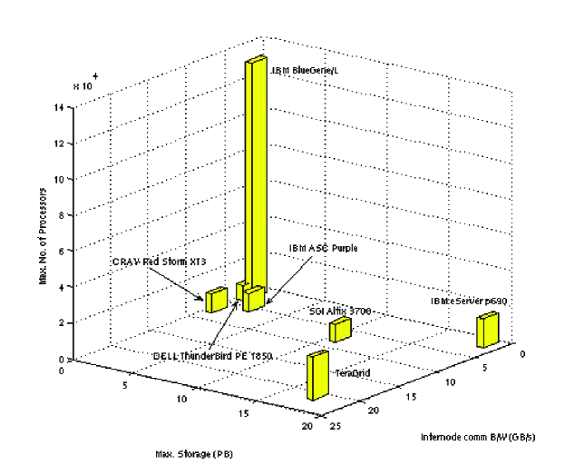
Figure 4: Internode communication bandwidth, maximum number of processors and maximum storage available for some of the recent supercomputers.

Table 4: Characteristic of some recent fast HPC architecture. UKWN signifies an unknown entity and N/A stands for Not Applicable.

Vendor	IBM	CRAY	DELL	SGI	IBM	TeraGrid
Model	BlueGene/L	Red Storm Cray XT$3$	Thunderbird - PowerEdge $1850$	NASA Columbia ALTIX $3700$	ASC Purple	TeraGrid
Available Memory(TB)	$16$	$31.2$	$24$	$20$	$40.96$	$>45$
Cache	$32$KB L1; $2$KB L2; $4$MB L3	$128$KB L1; $1$MB L2	$2$MB L2	$32$KB L1; $256$KB L2; $6$MB L3	$96$KB L1; $1.9$MB L2; $36$MB L3	N/A
Dist. Memory Architecture	Yes	Yes	Yes	No	Yes	Yes
Architecture Type	MPP	MPP	Cluster	MPP	MPP	Grid
Theoretical Peak (TFLOPS)	$360$	$41.47$	$64.512$	$60.96$	$111$	$>102$
Year (Ranking in Top500 list)	$2004$($\#1$), $2005$($\#1$)	$2005$($\#6$)	$2005$($\#5$)	$2005$($\#4$)	$2005$($\#3$)	$2006$(N/A)
Max. # processor	$131072$	$10368$	$8192$	$10240$	$10240$	$>24000$
Operating system	Linux	Linux/Catamount	Linux	Linux	AIX	Heterogeneous
Connection structure	$3$-D Torus, Tree Network	$3$-D Mesh $(27$x$16$x$24)$	Classified (Red) and Unclassified (Black)	Crossbar and hypercube	Bi-directional, Omega-based variety of Multistage Interconnect Network (MIN)	Heterogeneous (Myrinet, SGI NUMAlink, InfiniBand, IBM Federation, $3$-D torus, global tree, Quadrics, Cray Seastar, Gigabit Ethernet and Sun Fire Link)
Interconnect	Gigabit Ethernet	$100$ MB Ethernet	Infiniband	SGI Numalink, InfiniBand network, Gigabit Ethernet	Federation	Hub: CHI, ATL, LA, DEN, Abilene. (for connection between sites)
Memory bandwidth (GB/s)	$22.4$	$5.304$	$6.4$	$12.8$	$12.4$	N/A
Internode Comm. bandwidth (GB/s)	$\leq 1.05$	$6$	$1.8$	$6.4$	$4$	$10$-$30$ to Hub
Cost	$\geq$USD$1.5$ depending on configuration	UKWN	UKWN	UKWN	UKWN	N/A
Application specific	No	Yes	No	No	No	No
Storage (PB)	$0.4$	$0.24$	$0.17$	Online: $0.44$ Fibre channel RAID; Archive: $10$	$2$	Online:$3$; Mass:$>17$
Processor	PowerPC $440$	AMD x86–64 Opteron	Dual Intel Xeon EM64T	Intel IA-$64$ Itanium $2$	Power5	$8$ distinct architectures
Clock speed (GHz)/processor	$0.7$	$2.0$	$3.6$	$1.5$	$1.9$	N/A
Site	DOE/NNSA/ LLNL	Sandia National Laboratories	Sandia National Laboratories	NASA/Ames Research Center/NAS	Lawrence Livermore Computing	ANL/UC/IU/ NCSA/ORNL/ PSC/Purdue/ SDSC/TACC

In this section, we look at some of the HPC architectures that consists of MPP, Cluster and Grids. Fig. 3 and Fig. 4 shows the characteristics for some of the supercomputers. It is interesting to note that the number of processor used in recent architectures are increasing and hence the increase in the peak performance. However, this peak performance is not usually achievable because of other overheads such as communication between nodes and data access from external storage. The sustained performance of an architecture very much depends on the type of application that is run, which relies on algorithms, computational and communication complexity, size of data that needs to be processed or generated for visualization purposes. In general, to obtain more processing power, new architectures are using more processors with higher memory bandwidths compared to their predecessors. They also tend to have large main memory and storage space to solve large scale problems that incorporates high degree of abstraction and resolution size for better accuracy. In the following sections we look at some of the recent supercomputer characteristics in detail.

3.1 IBM (Blue Gene/L)

Blue Gene/L [42, 2, 65] compute chip is a dual processor (clock speed per processor $0.7$ GHz) system-on-a-chip capable of delivering an arithmetic peak performance of $5.6$ Gigaflops. It is a Massively Parallel Processor (MPP) with three-level on-chip cache that offers high-bandwidth and integrated prefetching cache hierarchy on L2 ($32$ KB), L3 ($4$ KB) to reduce memory access time. Memory to CPU bandwidth of $22.4$ GB/s is provided to serve speculative pre-fetching demands of two processors cores [65]. The Blue Gene can be scaled up to $65,536$ compute nodes yielding a theoretical peak of $367$ Teraflops and has storage space of $400$ Terabytes  . The nodes are interconnected through five networks: 1) a $3$-dimensional torus network for point-to-point messaging between computing nodes with a bandwidth of $0.175$ GB/s. If all six bidirectional links that connect to a given node are fully utilized, a bandwidth up to $1.05$ GB/s can be achieved; 2) a global collective network for collective operation over the entire application; 3) a global barrier and interrupt network; 4) a gigabit Ethernet for machine control; and 5) another gigabit Ethernet network for connection to other systems [2].

3.2 CRAY (Red Storm XT3)

Red Storm is a MPP supercomputer at Sandia National Laboratories, New Mexico. Red Storm was uniquely designed by Sandia and Cray, Inc. It runs on $10,368$ AMD Opteron microprocessor at a clock speed of $2$ GHz with a total memory of $31.2$ TB. Together with a two level-on-chip cache memory hierarchy, $128$ KB L1 and $1$ MB L2, and yields a theoretical peak of $41.47$ Teraflops. The system provides a maximum of $5.304$ GB/s data flow between the cpu and memory. It is constructed from commercial off-the-shelf parts supporting IBM-manufactured SeaStar interconnect chip. The interconnect chips, accompanies each of $10,368$ compute node processors and is a key to three-dimensional mesh that allows $3$-D representation of complex problems. The system has $6$ GB/s CPU memory bandwidth and a storage space of $240$ Terabytes.  This architecture was built specifically for running simulation for nuclear stockpile work, weapons engineering and weapons physics.

3.3 Dell Thunderbird

ThunderBird  is a supercomputer with cluster architecture at Sandia National Laboratory running on a single core SMP node with dual Intel Xeon EM64T processors. A total of $8,192$ processor at clock speed of $3.6$ GHz is used. ThunderBird has a $2$ MB L2 cache memory and $24$ Terabytes of main memory. With CPU memory bandwidth of $6.4$ GB/s it yields a theoretical speed of $64.5$ Teraflops. Thunderbird has an interprocessor communication bandwidth of $1.8$ GB/s over $4$ InfiniBand network and a storage space of $170$ Terabytes [69].

3.4 SGI (NASA Columbia ALTIX 3700)

NASA’s Columbia supercomputer is a MPP architecture with $10,240$ processor system comprising of twenty $512$-processor nodes. Twelve of which are SGI Altix $3700$ nodes, and the other eight are SGI Altix $3700$ Bx2 nodes. Each node is a shared memory, Single System Image (SSI) system, running a Linux based operating system. Four of the Bx2 nodes are linked to form a $2,048$ processor shared memory environment. It is powered by Intel IA-64 Itanium processor running at clock speed of $1.5$ GHz. it has three-level on-chip cache of $32$ KB L1, $256$ KB L2 and $6$ MB L3 with CPU memory bandwidth of $12.8$ GB/s. The system has a maximum theoretical peak of $60.96$ Teraflops. All the nodes are interconnected via SGI Numalink, InfiniBand network and gigabit ethernet network. It has an internode communication bandwidth of $6.4$ GB/s and a combined storage space of $10.44$ Petabytes.

3.5 IBM (ASC Purple)

Each IBM ASC Purple  node is a Symmetric multiprocessor (SMP) powered by $8$ Power5 microprocessor running at $1.9$ GHz, configured with $32$ GB of memory. The system at Lawrence Livermore Computing Laboratory has a total of $1,280$ nodes with a combined total memory of $40.96$ TB. It has three-level-on-chip cache memory, $96$ KB L1, $1.9$ MB L2, and $36$ MB L3 to reduce memory access time. A CPU memory bandwidth of $12.4$ GB/s comes together with a total number of $10,240$ processors, so the theoretical speed achievable by this system is $111$ Teraflops. The system also has a storage space of $2$ Petabytes. All of the $1,280$ nodes in IBM ASC Purple system are interconnected by dual plane federation (pSeries High Performance) switch [71]. The federation network can be classified as bidirectional, $\Omega-$based variety of Multistage Interconnect Network (MIN). Bidirectional here refers to each point-to-point connection between nodes comprised of two channels (full duplex) that can carry data in opposite directions simultaneously. MIN is used as an additional intermediate switch to scale the system upwards.

3.6 TeraGrid

TeraGrid ^, is an open scientific discovery infrastructure combining resources at nine partner sites to create an integrated, persistent computational resource. The partner sites are University of Chicago, Indiana University, Oak Ridge National Laboratory, National Center for Supercomputing Applications, Pittsburgh Supercomputing Center, Purdue University, San Diego Supercomputer Center, Texas Advanced Computing Center, and University of Chicago/Argonne National Laboratory. TeraGrid integrates data resources and tools, and high-end experimental facilities at all the partners’ sites using high-performance network connections. These integrated resources have a combined $102$ Teraflops of computing capability and more than $15$ Petabytes of online and archival data storage with rapid access and retrieval over high-performance networks. Researchers can access over 100 discipline-specific databases through TeraGrid. With this combination of resources, TeraGrid is the world’s largest distributed infrastructure for open scientific research.

3.7 Summary

In this section, we looked at some of the recent supercomputers and their characteristics. New supercomputers typically consume less energy with higher computing capability. For example, NEC Earth Simulator consumes $12,000$ kW power [22] compared to $1,800$ kW power [37, 42] by BlueGene/L each producing $35.86$ TeraFlops and $280.6$ TeraFlops respectively on LINPACK benchmark. Current HPC architectures have higher memory bandwidth, a large number of processors and large storage capacity compared to their previous generations. The current fastest supercomputer, IBM BlueGene/L, was built to provide cost effective performance but is not meant for all applications [42]. Here, a suitable parallel computing model can be used to determine how an application can be efficiently implemented on a given architecture. More importantly, performance of a given architecture depends on the configuration of the architecture and also the type of algorithm that is used.

It is also worth noting that aggregating HPC resources distributed across the WAN is becoming a trend in HPC as demonstrated by the TeraGrid infrastructure. This is in part contributed by the network technologies that are advancing at a faster rate now compared to a decade ago. The power of network, storage and computing resources are projected to double every $9$, $12$ and $18$ months, respectively. Improvements in wide area networking makes it possible to aggregate distributed resources in collaborating institutions to solve problems in the area of scientific computing using numerical simulation and data analysis techniques to investigate increasingly large and complex problems [25].

In the following section, we cover different parallel computing models that are used to develop high performance software that solve computationally intensive problems on HPC architectures efficiently.

4 Computational models

4.1 Background on models

It is important to have a clear picture of the problems and architectures in order to see the connection with the associated computational models and to see how the models have and can be evolved. In the previous two sections, we covered a variety of HPC challenge problems and described a number of HPC architectures that have been developed to address these challenges. In this section, we cover the development of computational models that connect the high-level problem solving environments and approaches to the lower-level architectural characteristics. We also see that computational models tend to put emphasis on the architectural parameters.

Figure 5: Characteristics of parallel architectures that are emphasized in many traditional parallel computing models.

It is common knowledge that a solution to any task begins with an algorithm, which realizes the computational solution. However, translating a problem to a computational algorithm requires a model of computation that defines an execution engine. Thus, a computational model plays an important role as a bridge between software and hardware.

A model is said to be more powerful than another if algorithms have a lower complexity in general on the machine. A computational model also guides in the high-level design of parallel algorithms. Models should balance between simplicity with accuracy, abstraction with practicality, and descriptivity with prescriptivity [62]. Models of parallel computation exists in several levels. They are classified as: specification models (e.g. Z , VDM , and CSP ); programming models (e.g. HPF , Split-C , and Occam ); cost models (e.g. PRAM [38], BSP [77], and LogP [29]); architecture models (e.g. message-passing, RPC, shared memory, semaphores, SPMD, MPMD) and physical models (e.g. distributed memory, shared memory, and cluster of workstations and Grid). Despite the well defined boundaries, there is some overlap by models: some specifications act as programming models; some cost models act as architectural models, etc [23]. In this section, we limit our discussion domain on the cost model for accurate prediction of parallel algorithm performance.

Many models have been developed for parallel architectures. The majority of these models emphasize on seven important architecture characteristics in parallel computing as depicted on Fig. 5.  [62] These are:

Computational parallelism

The number of processors, $p$, to be used in computation.

Network topology

Describes the inter-connectivity of processing nodes. Communication requirement of a parallel application should consider network topology of an architecture for efficient implementation.

Communication latency

Is the delay caused in accessing the non-local memory.

Communication overhead

Cost of message formation and injection of packets into the network.

Memory hierarchy

Is the different levels of memory from which data needs to be moved to reach the processor.

Communication bandwidth

Describes the bandwidth available for inter-processor communications.

Execution synchronization

The requirement for processors to wait until the required data has been received before proceeding with computations.

The Parallel Random Access Memory (PRAM) model was the most widely used model [38], with the assumption that all processors work synchronously and communication between processor are costless. As a result, the model has not been realistic in current parallel architectures, where cost of communication delay, asynchrony and memory hierarchy have far reaching impact on performance. These constraints in the PRAM model provided sufficient catalyst to develop models that emphasize on PRAM’s weakness. Many variants of the PRAM model have mushroomed ever since (e.g. Phase PRAM, APRAM, LPRAM, and BPRAM). We will discuss them later in this section. Other models that emphasize on weaknesses of the PRAM Model such as the Postal model [15], BSP (Bulk Synchronous Parallel)  [77] and LogP [29] considers communication costs such as network latency and bandwidth. Parallel hierarchical models such as Parallel Memory Hierarchy (PMH) [11], Parallel Hierarchical Memory model (P-HMM) [54], LogP-HMM and LogP-UMH [61] address the memory hierarchy in parallel computing. Table  LABEL:model_properties shows some important properties that are usually considered in parallel computing models and the properties are explained below:

Distributed/Shared memory

This property refers to type of memory used in a system that is supported by the model. Shared memory system have multiple CPUs all of which share the same address space. Whereas the distributed memory system has in each CPU its own associated memory. The CPU are connected by some form of network and exchanges data between their respective memory when required.

Synchronous/Asynchronous

This property identifies if a model supports synchronous or asynchronous algorithm.

Latency

Is the cost of accessing data in the memory (local, shared or distributed memory). This property has significant effect on performance of parallel algorithm. The cost increases with the distance from the data requesting processor.

Bandwidth

Bandwidth in a HPC architecture can be divided into two parts the memory and the interprocessor bandwidth. This bandwidth is not unlimited and is an important characteristic to consider particularly in distributed memory architecture.

Memory Hierarchy

This property denotes that the model takes into consideration different level of memory hierarchy such as registers, cache, main memory and secondary memory. This property is very important to accurately reflect performance of an algorithm.

Overhead

Is the communication overhead introduced by processor for message handling. It is defined to be the time the processor spends for sending and receiving message. This value depends on the communication protocol used.

Block transfer

This property takes into consideration the cost of latency incurred when a block of memory is accessed. In most architectures, cost of accessing the first address is expensive, but accessing subsequent addresses is considerably cheaper.

Algorithms

List of algorithms that have been implemented or its parallel complexity analyzed theoretically.

Architecture

Architectures used to analyze a particular model.

4.1.1 Parallel Random Access Machine (PRAM) model and it’s variants

The PRAM is an idealized parallel computing model that is widely used to assess theoretical performance of parallel algorithms. PRAM [38] is a shared memory model that has allowed development of architecture independent parallel algorithms. Known as an extension of RAM model, it mimics the processor part of RAM model. A constant cost of memory access and computation steps are assumed in this model. Since there maybe more than one simultaneous memory read operation and simultaneous memory write operation by processors, four different classes of PRAM model that define how this should be handled is introduced [51].

In the exclusive read, exclusive write (EREW PRAM) model, a memory can only be accessed (for reading or writing) by one processor at a time and it is the most restrictive model of the four. The second model known as concurrent read, exclusive write (CREW PRAM), allows a memory location to be accessed by more than one processor simultaneously but only for reading the contents of the locations. Memory access for writing can only be done one at a time. The exclusive read, concurrent write (ERCW PRAM) model, allows multiple processors to write but only one to read, this model is usually not considered because a machine powerful enough to support concurrent write should be able to accommodate concurrent read. This model is thus subsumed in the CRCW model. The fourth model, the concurrent read, concurrent write model (CRCW PRAM), allows memory locations to be accessed by more than one processor simultaneously for both reading and writing. For the concurrent write permissable model (ERCW and CRCW) extra specification is necessary to resolve how conflicts are overcome and what the final stored result would be.

Absence of consideration for communication delay, asynchrony, memory and network contention in PRAM has also contributed to its lack of success. Consequently, many variations of the PRAM model have been developed. The Phase PRAM [46] and APRAM [27] model incorporates aspects such as asynchrony of processes. The LPRAM [6] emphasizes on memory access. BPRAM (Block PRAM) [4], an extension of the LPRAM addresses communication latency by considering the reduced cost for distributing a contiguous block of data. Here we describe the purpose of the variants and describe the functionality it plays in producing better understanding in designing parallel algorithms and also in predicting performance of parallel programs.

Phase Parallel Random Access Machine (Phase PRAM)

The Phase PRAM [46] extends the PRAM model with partial asynchrony. Its machine consists of a shared global memory, a set of $p$ sequential processors, and a local memory for each processor. Computation is separated into a set of phases, and all processors execute asynchronously, each phase is later ended by an explicit synchronization. The cost of a synchronization step, $B(p)$, is dependent on the number of processors $p$. This model discourages too many inter-processor communication. Theoretical analysis and simulation have been carried out for prefix sum, list ranking, Fast Fourier Transform (FFT), bitonic merge, multiprefix, integer sorting and Euler tours. [46]

Asynchronous Parallel Random Access Machine (APRAM)

APRAM is a “fully” asynchronous model [27, 28]. The APRAM model consists of a global shared memory and a set of processes with their own local memories. The basic operations executed by the APRAM processes are called events. An APRAM computation is denoted as the set of possible serializations of events executed by the process. A virtual clock is associated with each serialization. This virtual clock assigns a time $t(e)$ to each event $e$. The clock ”ticks” when each process has executed at least one event. Events may be read and write events, which operate on the shared and local memory, or local events. All events are charged unit cost. The pair (round complexity, number of processes) is used to measure the complexity of an APRAM algorithm, where a round is defined as the sequence of events between two clock ticks in a computation. The round complexity for a computation is defined to be the maximum number of possible ticks for that computation. For an algorithm the round complexity is defined as the maximum round complexity over all of the possible computations [61]. Complexity of graph connectivity and asynchronous summation algorithms have been analyzed for this model.

Local-Memory Parallel Random Access Machine (LPRAM)

The LPRAM model [6] is a model that deals with bandwidth. It consists of a shared global memory and a set of processors with unlimited local private memory. The CREW PRAM is used to access global memory and is more time consuming. At every time step, each processor can perform either a communication step, in which it can write and then read a word from the global memory, or a computation step, which is an operation that accesses at most two words from its local memory. Algorithms for matrix multiplication, sorting and Fast Fourier Transform (FFT) have been implemented on a binary tree architecture.

Block Parallel Random Access Machine (BPRAM)

The BPRAM, which is an extension of LPRAM [4]. BPRAM takes into consideration the time saved in transmitting a contiguous block of data. The model allows the usage of communication latency and the number of processors and to determine the limits within which efficient parallel algorithms can be written without taking into account the details of the machine topology. Two parameters are used in the BPRAM model, $l$ for startup cost or latency and $p$ the number of processors, The cost of accessing local memory is taken in unit time. For reading and writing a block size $b$ of contiguous locations in global memory a cost of $l+b$ is charged. Theoretical analysis for parallel algorithms such as matrix multiplication, matrix transposition, rational permutation, permutation networks, FFT and sorting have been investigated.

Table 5: Properties incorporated in different models. In the table, a check mark indicate that the characteristic is included in the model.

Models	Distributed or Shared memory	Synchronous or Asynchronous	Latency	Bandwidth	Memory hierarchy	Overhead	Block transfer	Network topology	Architectures
PRAM	Shared	Synchronous							Had been applied to many architectures but not accurate.
Algorithms: Matrix multiplication, solving system of linear equation, sorting, FFT, Graph problems, etc.
Phase PRAM	Shared	Semi-asynchronous	✓						-
Algorithms: Prefix sum, list ranking, FFT, bitonic merge, multiprefix, integer sorting and Euler tours.
APRAM	Shared	Asynchronous							-
Algorithms: Graph connectivity and asynchronous summation.
LPRAM	Shared	Synchronous		✓					Binary tree.
Algorithms: Matrix multiplication, sorting and FFT.
BPRAM	Shared	Synchronous	✓				✓		-
Algorithms: Matrix (multiplication, transposition), rational permutation, permutation networks, FFT and sorting.
Postal model	Distributed	Asynchronous	✓						-
Algorithms: Broadcast and summation.
BSP	Distributed	Semi-asynchronous	✓	✓					Clusters, Network of workstations, multistage network etc.
Algorithms: NBody, Ocean Eddy, Minimum spanning tree (MST), Shortest path and Matrix multiplication.
D-BSP	Both		✓	✓					-
Algorithms: Sorting and routing.
E-BSP	Distributed	Semi-asynchronous	✓	✓				✓	Linear array and mesh network.
Algorithms: Matrix multiplication, routing problem, all-to-all broadcast and finite difference application.
LogP	Both	Asynchronous	✓	✓		✓			Hypercube (nCUBE/2), Butterfly (Monsoon), Torus (Dash), $3$D mesh (J-Machine), Fat-tree (CM-5)
Algorithms: Parallel sorting, broadcast, summation, Fast Fourier Transform (FFT), and LU Decomposition.
CGM	Both	Semi Asynchronous		✓					2D Mesh, hypercube and fat-tree.
Algorithms: Geometric algorithms (e.g. $3$D-Maxima, multisearch on balanced search tree,
$2$D-nearest neighbors of a point set etc.), Graph problems (List rankings,Euler tour construction,
tree contraction and expression tree evaluation, etc.).
PMH	Distributed	Asynchronous	✓	✓	✓	✓	✓		Tree, ring and 2-D Mesh.
Algorithms:
P-HMM	Distributed	Asynchronous			✓				-
Algorithms: Matrix transpose and list ranking
logP-HMM	Distributed	Asynchronous	✓	✓	✓	✓			Fat-tree (Thinking machine CM-5).
Algorithms: FFT and sorting
logP-UMH	Distributed	Asynchronous	✓	✓	✓	✓			Fat-tree (Thinking machine CM-5).
Algorithms: FFT and sorting

4.1.2 Postal Model

The Postal model [15] is a distributed memory model with the constraint that the point-to-point communication has latency $\lambda$. It can be regarded as a model described by two parameters:$p$ and $\lambda$, where $p$ is the number of processors. Several elegant optimal broadcast and summation algorithms have been designed based on this model, which were then extended for LogP model [29]. Algorithms other than broadcast and summation have largely not been presented for this model.

4.1.3 Bulk Synchronous Parallel (BSP) and it’s variants

BSP [77] model provides support for developing architecture dependent model, thus indirectly promotes wide spread software industry for parallel computing. It has a cost model which incorporates essential characteristics of parallel machines. A BSP program is one which proceeds in stages, known as superstep. A superstep consists of computation, communication and synchronization phases. In the first phase, processors compute using locally held dataset. Data are then communicated between the processors in the second phase. In the third phase,global synchronization is carried out, and this is to ensure all the messages involved in communication are received before moving on to the next superstep. BSP parameters $p$, $g$, and $L$ are used to evaluate performance of a BSP computer. $p$ represents number of processor, $g$ and $L$ represents network parameters. If maximum local computation in a step takes time $W$, and the maximum number of send or receive by any processor is $h$ then the total time for a superstep is given by $T=W+hg+L$. Algorithms for N-Body, ocean Eddy, minimum spanning tree (MST), shortest path, matrix multiplication, sorting and routing have been developed using this model. [70, 64, 74, 45]

LogP

The LogP model is motivated by current technological trends in high performance computing towards networks of large-grained sophisticated processors. The LogP model uses the parameters $L$ for an upper bound of latency for transmitting a single message, $o$ for computation overhead of handling message, $g$ a lower bound of time interval between consecutive message transmission at a processor and $P$ the number of processors. [29]. In contrast to the BSP model, it removes the barrier synchronization requirement (h-relation in BSP) and allows the processors to run asynchronously. The network of a LogP machine has a finite capacity such that at any time at most $\lfloor L/g\rfloor$ messages can be in transit from or to any processor. It can support both shared and distributed memory architecture. The LogP model encourages well-known general techniques of designing algorithms for distributed memory machines including exploiting locality, reducing communication complexity, and overlapping communication and computation. The LogP model also promotes balanced communication patterns by introducing the limitation on network capacity so that no processor is overloaded with incoming messages. Moreover, it is often reasonable to ignore parameter of $o$ in a practical machine, such as in a machine with low bandwidth (high $g$). Parallel complexity analysis for sorting, broadcast, summation, Fast Fourier transform (FFT) and LU decomposition have been developed and implemented on different architectures such as hypercube, butterfly, Torus, $3$D mesh, and Fat-tree [56].

Coarse Grained Multi Computer (CGM)

CGM [32, 33, 31, 30] is a version of BSP model, it allows only bulk messages to be sent in order to minimize message overhead costs. A CGM consists of a set of $P$ processors $P_{1},P_{2},\ldots,P_{n}$ processors. Each communication round consists of routing a single $h-relation$ message. All information sent from one processor to another processor is packed into one large message to reduce communication overhead. Thus the communication time in CGM computer is the same as BSP computer plus the packaging time. An optimal algorithm in CGM model is equivalent to minimizing the number of communication round as well as local computation time. The model also minimizes other important costs such as message overhead and synchronization time. Parallel complexity of geometric algorithms (e.g. $3$D-Maxima, multisearch on balanced search tree, $2$D-nearest neighbors of a point set etc.), graph problems (List rankings, Euler tour construction, tree contraction and expression tree evaluation) have been analyzed and implemented on architecture such as $2$D Mesh, hypercube and fat-tree.

Extended BSP (E-BSP)

The BSP as well as BPRAM assume that the time needed for communication is independent of the network load. The BSP model conservatively assumes that all $h$-relations are full $h$-relations in which all processors send and receive exactly h messages. Likewise, in the BPRAM it is assumed that sending one $m$-byte message between two processors takes the same amount of time as a full block permutation in which all processors send and receive a m-byte message. The E-BSP model[53] extends the basic BSP model to deal with unbalanced communication patterns, i.e., communication patterns in which the processors send or receive have different data size. Like BSP, the E-BSP model is strongly motivated by various routing results. Furthermore, the cost function supplied by E-BSP generally is a non-linear function that strongly depends on the network topology. Several algorithms that uses this model such as routing problem, all-to-all broadcast operation, matrix multiplication and finite difference application have been developed.

D-BSP

Decomposable Bulk Synchronous Parallel(D-BSP)[18, 75] is a variant of BSP to capture some aspects in network proximity. A set of n processor/memory pairs that can be partitioned as a collection of clusters, where each cluster is independent of the other and is characterized by its own bandwidth and latency parameters. The partition of clusters can change dynamically within a pre-specified set of legal partitions. The advantage is that communication patterns where messages are confined within small clusters have small cost. Thus the model is claimed to represents realistic platforms unlike as in standard BSP. This advantage translates into higher effectiveness and portability of D-BSP over BSP.

4.1.4 Memory hierarchy models

As technology in electronics matures, different components of computer improves at different rates. In particular, the rate of increase in processor speed is far more rapid compared to the increase in bandwidth for local memory. Memory hierarchy was introduced in computer architecture to assist in keeping up with the memory request rate from central processing unit. This allows, data to be accessed from the fastest memory, such that the average time for fetching data is reduced significantly. Each level of memory in the memory hierarchy has its own costs and performance. Thus to reduce cost, memory that are more expensive to build is used stringently. At the lowest level, CPU registers and caches are built with the fastest and most expensive memory. At a higher level, inexpensive but slower disks are used for external mass storage [80]. Models that do not reflect the usage of memory hierarchy is most likely to be inaccurate, because of the presence of registers, caches, main memory and disks. Programs that are tuned to a particular architecture by considering memory hierarchy can produce significant speed up, thus it is important to write programs that takes memory hierarchy into consideration. As a result, computational models to reflect performance of these programs are established. Data movement to and from processors, cache memory and main memory incur some cost depending on the distance from the processing unit. In the RAM model, there is no concept of memory hierarchy; each memory access is assumed to take one unit of time. This model “may” be appropriate for small size of problem that can fit into the main memory, but as mentioned earlier registers, cache and disks can contribute to inaccuracy. Many variant of hierarchical memory model has been introduced, in this section we discuss some of the models.

Parallel Hierarchical Memory Model (P-HMM)

The Hierarchical Memory model (HMM) introduced by Agrawal et. al  [3] charges a cost of $f(x)$ to access memory location $x$ instead of a constant time taken in the Random Access Machine (RAM) [8] model. In HMM the concept of block memory transfer to utilize spatial locality in algorithms was not introduced but the Hierarchical Memory Model with Block Transfer (HMBT) [5] takes this factor into consideration. The P-HMM model is also known as the parallel I/O model [81, 79]. This model considers data that resides in hardisk rather than just the main memory. For allowing parallel data transfer, the P-HMM was introduced. It has $P$ separate memories connected together at the base level of the hierarchy. Each $P$ hierarchies can function independently, and communication between hierarchies takes place at the base memory level. The $P$ base memory level locations are interconnected via a network and the $P$ hierarchies can each function independently. This model also assumes that the $P$ base memory levels are interconnected via a network such as a hypercube or cube-connected. [81]

Parallel Memory Hierarchy (PMH)

The PMH model[11] uses a single mechanism to model the costs of inter-processor communication and memory hierarchy. A parallel computer is modeled as a tree of memory modules with modules at the leaves as processors. The leaf module performs computation while other modules holds data. Data in a module is partitioned into blocks and it is the basic unit of data transfer between a child and its parent. Communication between two processor resembles somewhat like a fat-tree model but differs by having memory and messages made explicit. The model has four parameters for each module $m$, the block-size $s_{m}$ (number of bytes per block of $m$ ); the block-count $n_{m}$ (number of block that fits in $m$); the child-count $c_{m}$ (number of children $m$ has); transfer time $t_{m}$ (number of cycles it takes to transfer a block between $m$ and its parent). Appropriate tree structure and parameter values should be chosen confirming to the machines communication capabilities and memory hierarchy.

LogP-HMM

This model consist of two parts: the network and the memory part. The network part is captured by LogP model and the memory part by the Hierarchical Memory Model (HMM) thus the name LogP-HMM. [61] This model is defined much like a P-HMM model. It consists of a set of asynchronously executing processors, each with an unlimited memory. Local memory is organized as a sequence of layers with increasing size, where size of memory block is $1$ and the size of layer $i$ is $2^{i}$. The cost of accessing a memory location at address $x$ is $log\text{ }x$. The processors are connected by LogP network at level $0$. It also assumes that the network has finite capacity such that at any time at most $\lfloor\frac{L}{g}\rfloor$ messages can be in transit from or to any processor.

LogP-UMH

The primary difference between LogP-UMH [61] and LogP-HMM is that the former uses memory organized as in Uniform Memory Hierarchy (UMH) [10]. The UMH model is an alternative model for multilevel memories and is an instance of the more general Memory Hierarchy (MH) [10] model. The MH model consists several memory module levels and each module is characterized by three parameters: $s_{l}$ (the number elements in a block), $n_{l}$ (the number of blocks), and $b_{l}$ (the time to move a block of size $s_{l}$ from level $l$ to level $l+1$). $UMH_{\alpha,\rho,f(l)}$ is a simplification of MH model that defines the $l$th memory level $M(l)$ as $M(l)=\langle s_{l},n_{l},b_{l}\rangle$ = $\langle\rho^{l},\alpha\rho^{l},\rho^{l}f(l)\rangle$, where $\alpha$ and $\rho$ are integer constants. That is, the $l$th memory level consists of $\alpha\rho^{l}$ blocks, each of size $s(l)=\rho^{l}$, and is connected to levels $l-1$ and $l+1$. Each block on level $l$ can be randomly accessed as a unit and transferred to or from level $l+1$ with a cost of $\rho^{l}f(l)$, where $f(l)$ is a well behaved function for the level $l$ and is known as the transfer cost function ($\frac{1}{f(l)}$ is the bandwidth).

4.2 Models for Wide Area Network (WAN)

Parallel applications are traditionally run on dedicated supercomputers where resources are usually homogeneous, with predictable network behavior and are usually allocated entirely for a single application without contention from other applications. Developing computational model for grid environment is difficult due to heterogeneous computing resources, heterogeneous network (bandwidth and latency), resource contention from different application, reliability and availability issues. However, attempts are already made to estimate the behavior/performance of parallel application on this environment. In this section we discuss some of the works.

4.2.1 Heterogeneous Bulk Synchronous Parallel- k (HBSP^k)

The k-Heterogeneous Bulk Synchronous Parallel [82] (HBSP^k) model is a generalization of the BSP model [77] of parallel computation. This model is characterized by eleven parameters as shown in Table  LABEL:hbspk which can be used to accommodate different architectures. HBSP^k is claimed to provide sufficient information for developing parallel applications on wide-range of architecture such as traditional parallel architecture (supercomputers), heterogeneous clusters, the internet and computational grids. Each of these system are then grouped together based on their ability to communicate with each other.

Table 6: Parameters used in HBSP^k model.

Parameters	Description
$M_{i,j}$	a machine’s identity, with $0\leq i\leq k$, $0\leq j\leq m_{i}$.
$m_{i}$	number of HBSPk machines on level $i$.
$m_{i,j}$	number of children of $M_{i.j}$.
$g$	A bandwidth indicator that reflects the speed at which the fastest machine can inject packets into the network.
$r_{i,j}$	The speed relative to the fastest machine for $M_{i,j}$ to inject packets into the network.
$L_{i,j}$	overhead to perform a barrier synchronization of the machines in the subtree of $M_{i,j}$.
$c_{i,j}$	fraction of the problem since that $M_{i,j}$ receives.
$h$	size of a heterogeneous $h$-relation.
$h_{i,j}$	largest number of packets sent or received by $M_{i,j}$ in a superi-step.
$S_{i}$	number of superi-step.
$T_{i}(\lambda)$	execution time of superi-step.

HBSP^k refers to a class of machines with at most $k$ levels of communication. When $k=0$ it represents a single processor system, for $k=1$ it represents class of machines which consists of at most one communication network, as an example, a HBSP¹ machine may include a single processor systems(i.e. HBSP⁰), traditional parallel machines, and heterogeneous workstation clusters. In general, HBSP^k systems include HBSP^k-1 computers as well as machines composed of HBSP^k-1 computers and the relationship of the machine classes is HBSP${}^{0}\subset$ HBSP¹ $\cdots\subset$HBSP^k.

A HBSP^k machine is represented by a tree $T=(V,E)$. Each node of $T$ represents a heterogeneous machine. The level of root is equal to the height of the tree, $k$ and root $r$ of tree $T$ is known as a HBSP^k machine. If $d$ is the length of the path from the root $r$ to a node $x$, the level of node $x$ is $k-d$. Thus nodes at level $i$ of tree $T$ are HBSPⁱ machines. Fig. 6 shows the HBSP² cluster and it’s tree representation in this model. Machines are indexed according to level $i$, $0\leq i\leq k$, are labeled $M_{i,0},M_{i,1},\ldots,M_{i,m_{i}-1}$, where $m_{i}$ represents the number of HBSPⁱ machines. Machine $M_{i,j}$ of a HBSP^k computer, where $0\leq j\leq m_{i,j}$ is a cluster with identity $j$ on level $i$. A machine at level $i$ of tree $T$ is taken as a coordinator nodes of machines at level $i-1$. This coordinators act as a representative for their cluster during inter-cluster communication or represent the fastest computer in their subtree to increase algorithmic performance. Cost of computation by HBSP^k machine is calculated directly at each level $i$.

An HBSP^k computation consists of a combination of superⁱ-steps and during a superⁱ-step, each level $i$ node performs asynchronously some combination of local computation, message transmission to other level $i$ machines, and message arrivals from its peers. A message that is sent in one superⁱ-step is guaranteed to be available to the destination machine at the beginning of the next superⁱ-step. This is achieved by having a global synchronization of all the level $i$ computers after each superⁱ-step. A HBSP¹ machine has to perform communication to transfer data, unlike HBSP⁰ machine where communication and synchronization is not applicable. A HBSP¹ computation resembles a BSP computation but only differs in how HBSP¹ algorithm delegates more work to the faster processor. The HBSP² machine consists of super¹-steps and super²-steps. In the super²-step, the coordinator nodes for each HBSP¹ cluster performs local computation and/or communication between other level $1$ coordinator nodes.

The value of $r_{i,j}$ for the fastest machine (root) is normalized to $1$. Thus other machines, $M_{i,j}$, are said to be $t$ times slower than the fastest machine if $r_{i,j}=t$. The $c_{i,j}$ parameter is used for load balancing purposes, it provides problem size to machine $M_{i,j}$ that is proportional to its computational and communication capabilities. The HBSP^k model does not mention about how to find values of $c_{i,j}$, and assumes that the cost have been determined beforehand.

\psfrag{M0,0}{$M_{0,0}$}\psfrag{M0,1}{$M_{0,1}$}\psfrag{M0,2}{$M_{0,2}$}\psfrag{M0,3}{$M_{0,3}$}\psfrag{M0,4}{$M_{0,4}$}\psfrag{M0,5}{$M_{0,5}$}\psfrag{M1,0}{$M_{1,0}$}\psfrag{M1,1}{$M_{1,1}$}\psfrag{M1,2}{$M_{1,2}$}\psfrag{M2,0}{$M_{2,0}$}\psfrag{HBSP2}{HBSP${}^{2}$}\psfrag{super0-steps}{super${}^{0}$-steps}\psfrag{super1-steps}{super${}^{1}$-steps}\psfrag{super2-steps}{super${}^{2}$-steps}\psfrag{k=2}{$k=2$}\psfrag{(M1,0)}{($M_{1,0})$}\psfrag{(M1,2)}{($M_{1,2})$}\psfrag{(M2,0 & M1,1)}{($M_{2,0}$ \& $M_{1,1}$)}\psfrag{An HBSP2 cluster}{An HBSP${}^{2}$ cluster}\psfrag{Tree representation of HBSP2 cluster}{Tree representation of HBSP${}^{2}$ cluster}\includegraphics[height=169.83493pt,width=433.62pt]{Hbsp2.eps}

Figure 6: An HBSP^k cluster and it’s tree representation.

The execution time of superⁱ-step is given by,

$$T_{i}(\lambda)=w_{i}+gh+L_{i,j}.$$

where, $w_{i}$, represents the largest amount of local computation performed by an HBSPⁱ machine, $h$=max{$r_{i,j}\cdot h_{i,j}$}, is the heterogeneous $h$-relation with $h_{i,j}$ the largest number of messages sent or received by $M_{i,j}$, where $0\leq j<m_{i}$ and $gh$ as the routing cost. If $S_{i}$ is the number of superⁱ-steps, where $1\leq i\leq k$. The execution time of an HBSP^k algorithm is the total time taken by superⁱ-steps. Thus the overall cost given by this model is,

$$\sum_{\lambda=1}^{S_{1}}T_{1}(\lambda)+\sum_{\lambda=1}^{S_{2}}T_{2}(\lambda)+\ldots+\sum_{\lambda=1}^{S_{k}}T_{k}(\lambda).$$

This model shows factors that are important to be considered when designing HBSP^k application. Similar to BSP model, to minimize the execution time, programmer must consider, $(i)$ balancing the local computation of the HBSP^k machines in each superⁱ-step, $(ii)$ balance the communication between the machines, and $(iii)$ minimize the number of superⁱ-steps.

The utility of the model is demonstrated through the design of collective communication algorithms such as gather, scatter, reduction, prefix sums, one-to-all broadcast and all-to-all broadcast. Two simple design principles are used, i.e. the root of a communication operation must be a fast node and faster nodes receive more data than the slower nodes. To validate the predictions of the HBSP^k two experiments were carried out for both designs. It was found that not all algorithms benefits on a heterogeneous environment. For example, broadcast (one-to-all and all-to-all) algorithm developed using the two design principles shows negligible benefits. The predicted and actual values for one-to-all-broadcast communication are shown in Table  8 and Table  8 respectively. $p$ is the number of processors, $T_{s}$ and $T_{f}$ denote the execution time assuming a slow and a fast root node, respectively. $T_{b}$ is the runtime for balanced workload (each node has same the amount of workload). This is because a broadcast requires each machine to possess all of the data elements at the end of the operation and clearly slowest machine effects the overall performance. Thus the conclusion driven was, any collective operation that require nodes to possess all of the data items at the end of operations will not be able to exploit heterogeneity.

The plus point for this model is that HBSP^k gives a single system image of a heterogeneous platform by incorporating salient features of the underlying machines (characterized by a few parameters). This keeps an application developer away from non-uniformity of the underlying architecture. The model however does not include fault tolerance issues. Some of the parameters used are assumed to be constant, but this is not the case for heterogeneous machines that are distributed geographically apart. Communication between nodes depend on the network conditions, furthermore the load of processing nodes are not constant on Grids.

Table 7: Table shows the predicted values for the one-to-all broadcast communication using the $HBSP^{k}$ model.

	problem size (in KBs)
	$100$	$200$	$300$	$400$	$500$	$600$	$700$	$800$	$900$	$1000$
$p=10$
$T_{s}$	$0.238$	$0.402$	$0.566$	$0.729$	$0.893$	$1.057$	$1.221$	$1.385$	$1.549$	$1.712$
$T_{f}$	$0.176$	$0.278$	$0.380$	$0.482$	$0.584$	$0.686$	$0.788$	$0.890$	$0.992$	$1.094$
$T_{b}$	$0.176$	$0.278$	$0.380$	$0.482$	$0.584$	$0.686$	$0.788$	$0.890$	$0.992$	$1.094$

Table 8: Table shows the actual execution time for the one-to-all-broadcast communication using the $HBSP^{k}$ model.

	problem size (in KBs)
	$100$	$200$	$300$	$400$	$500$	$600$	$700$	$800$	$900$	$1000$
$p=10$
$T_{s}$	$1.426$	$1.769$	$1.452$	$1.770$	$2.310$	$3.588$	$3.332$	$3.877$	$4.489$	$5.061$
$T_{f}$	$0.450$	$0.862$	$1.266$	$1.537$	$2.041$	$2.435$	$3.152$	$3.573$	$4.212$	$4.773$
$T_{b}$	$0.410$	$1.13$	$1.134$	$1.766$	$1.839$	$2.676$	$3.269$	$3.633$	$4.476$	$4.952$

4.2.2 Bulk Synchronous Parallel-GRID (BSPGRID)

BSPGRID [78] is a model based on BSP model for grid based parallel algorithms. It extends the Bulk Synchronous Parallel Random Access Machine (BSPRAM) [73] model which is an extension of BSP model with shared memory to reduce the complexity involved in algorithm design and programming. A BSPGRID is a collection of processor with limited memory units, a shared memory with unlimited capacity, and a global synchronization mechanism. The shared memory is likely to be a collection of disk units in this model. At the end of each supersteps processors are globally synchronized and the contents of all local memories are discarded. This is in contrast with BSP model where there is a persistency of data at processor nodes between supersteps. The concept of virtual processors is used when the problem size is larger than memory capacity at the processing nodes. This implies that each physical processing units may be required to perform work of multiple virtual processors sequentially in a particular superstep. Processor reliability and availability is taken into consideration by allowing the number of physical processor to vary between supersteps. A recovery protocol is also provided in case processors fail unexpectedly during supersteps. An additional synchronization barrier is introduced and the work of failed processors is rescheduled after the barrier. It is not mentioned how the implementation of shared memory will be done. However, a centralized shared memory implementation would cause communication bottleneck at the master processor, thus a likely solution is to implement virtual shared memory distributed over the grid [63]. The BSPGRID cost model has four parameters as shown in Table  LABEL:bspgrid. The model allows time and work cost to be predicted for an algorithm. The time cost is defined as the best performance that can be achieved if enough processors are used to solve a problem. The work cost is defined as the processor-time product of the algorithm.

Table 9: Parameters used in BSPGRID model.

Parameters	Description
$M$	the amount of memory per processor in words.
$g$	the cost of shared memory access per word.
$l$	the cost of synchronization.
$N$	the problem size in words.

The time cost of a superstep is defined to be:

$$T=w+gh+l.$$

where $w$=$max_{i}w_{i}$, $h$ = max $h_{i}^{in}$+ max $h_{i}^{out}$, $w_{i}$, is defined as the cost of computation on processor $i$, $h_{i}^{in}$, is the number of words read from the shared memory to processing unit $i$, $h_{i}^{out}$, is the number of words written to shared memory from unit $i$. The work cost of a superstep is defined to be:

$$W=\upsilon T.$$

where, $\upsilon$, is the number of processors used during the superstep. It is noteworthy that these costs are similar to the PRAM model. The cost of an algorithm is taken as sum of the costs of all of its supersteps. The unit of the cost model is taken as the cost of a single computational operation. The value of $g$ and $l$ are normalized to this unit. A BSPGRID computer is defined as $BSPGRID(M,g,l)$ with fixed parameters $M$, $g$ and $l$. The number of processing unit is fixed and this number is derived from the value of $M$, $N$ and the algorithm used. Execution time of an algorithm with time cost $t$ and work cost $c$ on a $p$ processor machine that can emulate BSPGRID machine is given by $T(p)=(c-t)/p+t$. Computational complexity for matrix multiplication on grid was derived using this model. This model does not take into consideration the network and processing units heterogeneity which is an important aspect of Grid.

4.2.3 Dynamic BSP

This model is a modification of BSPGRID and it addresses the heterogeneity issues, fault tolerance and also provides the ability to spawn additional processes within supersteps when it is required.

Dynamic BSP [63] uses task-farm model to implement BSP supersteps, where individual tasks are represented as virtual processors. The data bottleneck problem of task-farm model is countered by using a master processor known as task server, worker processors and a data server(implemented either as a distributed shared memory or remote/external memory). Fig. 7 shows the difference between BSP computation and the Dynamic BSP computation. The master processor deals with task scheduling, memory management, and resource management. At the beginning of each superstep the master processor distributes a virtual processor number to each physical processor.

This virtual processor in turn fetches local data from data server, performs computations, write the output to the data server and informs the master processor that it has finished the task. The master processor which maintains a queue of pending virtual processors dynamically assigns them to waiting physical processors. When all the virtual processor have been executed in a particular superstep, the global shared memory is restored to a consistent state and the next superstep commences. The task farm approach used in this model hides heterogeneity across the grid by choosing the number of virtual processor to far exceed those of the physical processors (this approach is known as parallel slackness).

Figure 7: The difference between standard BSP computation and Dynamic BSP computation.

Fault tolerance is dealt by using timeouts, when time has exceeded the timeout period, the physical processor is considered to have died and the work is reallocated to another physical processor within the same superstep as shown in Fig. 7. This model also allows the virtual processors to spawn other virtual processors (child process). However, the child creation process has to be registered at the master processor, where the virtual process sends a message to master requesting it to spawn one or more children. The standard cost model for BSP is said to be suitable for dynamic BSP even though the value of parameters $g$ and $l$ will vary significantly between grid nodes. The author claims that using task-farm approach together with the use of parallel slackness would make it reasonable to utilize the measured values for $g$ and $l$ (suitably averaged) for predicting cost.

4.2.4 Parameterized LogP (P-logP)

The parameterized LogP (P-LogP) model [59] is an extension from LogP [29] and LogGP [9] model to accurately estimate the completion time of collective communication on a wide area systems (hierarchical systems). The existing models such as LogP model are inaccurate for collective communication on hierarchical systems with fast local networks and slow wide-area networks. This is because they use constant values for overhead and gap, also LogP is restricted to short messages while LogGP adds the gap per byte for long messages, assuming linear behavior. Both this models do not handle overhead for medium sized to long messages correctly and do not model hierarchical networks. The P-LogP model uses different sets of parameters for both networks, and consists of five parameters as shown in Table  LABEL:Plog_P. This model uses parameters as a function of message size and uses measured values as input. A network $N$ is characterized as $N=(L,os,or,g,P)$. The Gap parameter, $g(m)$ is also known as the reciprocal value of the end-to-end bandwidth from process to process for messages of size $m$. This parameter models the time a message “occupies” the network, as such the next message cannot be sent before $g(m)$ time. Hence, $r(m)=L+g(m)$ is the time the receiver has received the message. The latency $L$ on the other hand can be viewed as time taken for the first bit of message to travel from sender to receiver. This model is depicted in Fig. 8, values of these parameters are obtained from empirical studies.

Table 10: Parameters used in P-LogP model.

Parameters	Description
$P$	Number of processors.
$L$	End-to-end latency from process to process (it combines all contributing factors such as copying data to and from network interfaces and transfer over the physical network).
$os(m)$	Send overhead (time the CPUs are busy sending messages as a function of message size).
$or(m)$	Receive overhead (time the CPUs are busy receiving messages as a function of message size).
$g(m)$	Gap (minimum time interval between consecutive message transmissions or receptions along the same link or connection as a function of message size).

When a sender sends multiple messages in a row, the latency cost contributes only once to the completion time but the gap values of all messages sum up as, $r(m_{1},\ldots,m_{n})=L+g(m_{1})+\ldots+g(m_{n})$.

\psfrag{g(m)}{$g(m)$}\psfrag{=s(m)}{$=s(m)$}\psfrag{sender}{sender}\psfrag{os(m)}{$os(m)$}\psfrag{time}{time}\psfrag{or(m)}{$or(m)$}\psfrag{time}{time}\psfrag{receiver}{receiver}\psfrag{L}{$L$}\psfrag{+}{$+$}\psfrag{g(m)}{$g(m)$}\psfrag{=r(m)}{$=r(m)$}\includegraphics[height=144.54pt,width=238.49121pt]{PlogP.eps}

Figure 8: Message transmission in parameterized LogP.

For clustered wide area systems, two parameter sets are used, i.e for LAN and WAN with subscript $l$ and $w$ respectively. For a local area network, the time taken for the receiver to receive the message is given by: $r_{l}(m)=L_{l}+g_{l}(m)$ and the time taken for sending a message of size $m$ is given by: $s_{l}(m)=g_{l}(m)$. For wide area transmission, there are three steps: the sender sends message to its gateway, this gateway sends the message to the receiver’s gateway and finally the receiver’s gateway sends the message to the receiving node, refer Fig. 9. The value of $r_{w}$ depends on wide area bandwidth and is expressed as an analogy to $r_{l}$. Value of $s_{w}$ is determined by wide-area overhead $os_{w}(m)$ or local-area gap $g_{l}(m)$, whichever is higher. Thus the equations for wide-area case is: $s_{w}(m)=max(g_{l}(m),os_{w}(m))$ and $r_{w}(m)=L_{w}+g_{w}(m)$.

Performance model for single layer broadcast algorithm is given as $T=(k-1)\cdot\gamma(m)+\lambda(m)$ for $k$ message segment of size $m$. Here, latency $\lambda(m)$ and gap $\gamma(m)$ is of a broadcast tree analogous to $L$ and $g(m)$ for a single message send. $\lambda(m)$ denotes time taken for message to be received by all nodes, after root process starts sending it. $\gamma(m)$ is the time interval between the sending of two consecutive segments (indicates the throughput of a broadcast tree). For example values of $\gamma(m)$ and $\lambda(m)$ for flat WAN tree used in MagPIe [58] is:

$$\gamma(m)=\text{max}(g(m),(P-1)\cdot s(m)),$$

$$\lambda(m)=(P-2)\cdot s(m)+r(m).$$

Here, $\lambda(m)$ is the maximum of the gap between two segments of size $m$ sent on the same link and the time the root needs for sending $(P-1)$ times the same segment on disjoint links. The corresponding value for $\lambda(m)$ is the time at which a message segment is sent to the last node, plus the time it is received.

For general tree shape, upper bounds for both parameters can be expressed depending on the degree $d$ and height $h$ of a broadcast tree:

$$\gamma(m)\leq\text{max}(g(m),or(m)+d\cdot s(m)),$$

$$\lambda(m)\leq((d-1)\cdot s(m)+r(m)).$$

Here, $\lambda(m)$ is the maximum of the gap caused by the network, and the time a node needs to process the message. For intermediate nodes, this is the time to receive the message plus the time to forward it to $d$ successor nodes (for the root and for the leaf nodes, it is either one of both).The exact value of $\lambda(m)$ depends on the order in which the root process and all intermediate nodes send to their successor nodes and which path leads to the node that receives the message last.

\psfrag{Nodes}{Nodes}\psfrag{Gateway}{Gateway}\psfrag{LAN}{LAN}\psfrag{WAN}{WAN}\includegraphics[height=144.54pt,width=238.49121pt]{Cluster_LAN_WAN.eps}

Figure 9: Clustered wide area system.

P-LogP model is used to optimize four type of collective communications, namely broadcast, scatter, gather and all-gather in the MagPIe [58] message passing library.

4.3 Summary

In general, it is clear that all the computational models are trying to incorporate factors that effect data movements to accurately predict performance of parallel algorithms. A pattern that we observe in the traditional models is that they tend to focus on architectural parameters only rather than on both the algorithmic and architectural parameters. On WAN, factors that contribute to performance of inter-processor communication change very rapidly due to shared network and shared computing resources. As a result, it is impossible to predict performance of parallel applications accurately. However, it is very important to have some idea of the behavior of the WAN before a parallel application is deployed on it. We also see that the trend in computational models for WAN are to emphasize more towards tuning different types of communication that is frequently used in parallel algorithms by using empirically gathered information. This makes sense because the main bottleneck in parallel computing over WAN is the communication phase, assuming computational resources are reserved (available unconditionally without any failure) in advance for usage. There are many other factors that contribute to the performance of parallel programs on the WAN, and it is impossible at least at the moment to include all the factors and find an optimal solution in real time to obtain good speedup for parallel applications. It is also worth noting that the use of stochastic approach for computational models may be inevitable because of the unpredictable nature of the computational resources and the WAN.

5 Programming Libraries

Programming libraries play a very significant role in simplifying complexity involved in writing parallel programs. These libraries provide frequently used commands for developing parallel applications on HPC architectures. Historically, the main focus of programming language development has been on expressibility, and providing constructs which translate and preserve algorithmic intentions. However, lately the focus of language development has begun to include performance issue in addition to expressibility [62]. Performance issues are usually related to efficiently moving data. The cost of moving data between memory or storage to processing units and between processing units usually contributes considerably to the total computation time. In order to reduce this cost, many new algorithms (e.g. for collective communication) uses performance model to assist in tuning the parameters used for the communication [58].

In this section, we study some parallel programming libraries commonly used for parallel computing in System Area Network (SAN), Local Area Networks (LAN) and Wide Area Networks (WAN).

5.1 Parallel Virtual Machine (PVM)

PVM is a set of software tools and libraries that emulates a general-purpose, flexible, heterogeneous computing framework on an interconnected computers of varied architecture . The system is composed of two parts: 1) A daemon, called pvmd3 that resides on all computing nodes which makes up the virtual machine. Daemon can run on heterogeneous distributed computing nodes connected by different type of network topology. 2) An API that contains a library of PVM interface routines required to communicate between processes in an application. Processes can interact between each other via message passing where messages are send to and received using unique “task identifiers” (TIDs) which are the identifier for all PVM tasks in a parallel application. PVM supports C, C++ and Fortran languages. [43]

5.2 Message Passing Interface (MPI)

Message Passing Interface (MPI)  is a successful community standard for the extended portable message passing model of parallel communications. MPI is a specification and not a particular implementation. There are many implementation of MPI such as MPICH, LAM/MPI (runs on networks of Unix/Posix workstations), MP-MPICH (runs on Unix systems, Windows NT and Windows 2000/XP Professional), WMPI runs on Windows platform and MacMPI (MPI implementation for Macintosh computers). A more complete list of MPI implementation is available at LAM website . The most popular parallel implementation of these is the MPICH from Argonne National Laboratory. A correct MPI program should be able to run on all MPI implementation without change. The standard includes point-to-point communication, collective communication, process groups, communication contexts, process topologies, environmental management and inquiry, bindings for Fortran77 and C and also profiling interface. In message passing model each process executing in parallel have separate address spaces. It however does not include explicit shared-memory operations; operations that require more operating system support than is currently standard: e.g. interrupt-driven receives, remote execution, or active messages;program construction tools; debugging facilities; explicit support for threads; support for task management; and I/O functions [49].

5.3 Paderborn University BSP (PUB)

The Paderborn University BSP library is a C communication library based on BSP model. This implementation supports buffered as well as unbuffered non-blocking communication between any pair of processors. It also provides nonblocking collective communication operation such as broadcast, reduce and scan on any arbitrary subsets of processors. These primitives are however not available on Oxford BSP toolset or Green BSP library. Another different aspect of PUB is the possibility to dynamically partition the processors into independent subsets. As such PUB allows support for nested parallelism and subset synchronization. PUB also supports a zero-cost synchronization mechanism known as oblivious synchronization. The concept of BSP objects is introduced in PUB which serve three purposes. They are used to distinguish the different processor groups that exist after a partition operation, for modularity and safety purposes and can be used to ensure that messages sent in different threads do not interfere with each other and that a barrier synchronization executed in one thread does not suspend the other threads running on the same processors [20]. The most useful feature of BSP library variants compared to other model is the ability to construct a cost function using BSP parameters (p,r,g,l) which represents number of processors, computing rate , communication cost per data word and global synchronization cost respectively to predict performance and scalability of parallel programs. Other programming libraries that are conceptually based on BSP model include BSPlib [52], Green BSP [47], xBSP [57], and BSPedupack [19].

5.4 MPICH-G2

MPICH-G2 [55, 39] is a grid enabled implementation of the Message Passing Interface (MPI) that allows a user to run MPI programs across multiple computers at different sites using the same commands that would be used on a parallel computer. This library extends the Argonne MPICH implementation of MPI to use services provided by the Globus grid toolkit for authentication, authorization, resource allocation, executable staging, and I/O as well as process creation, monitoring, and control. Various performance critical operations, including startup and collective communication, are configured to exploit network topology information. The library also exploits MPI constructs for performance management, e.g., the MPI communicator construct is used for application-level discovery of both network topology and network quality-of-service. Adaptation is then performed for both the information. The major difference between MPICH-G2 and its predecessor MPICH-G is that the Nexus component which provided the communication infrastructure has been removed. The MPICH-G2 now handles communication directly by re-implementing Nexus with other improvements. This improvements include increased bandwidth, reduced latency for intra-machine, more efficient use of sockets, support for MPI_LONG_LONG and MPI-2 file operations and added C++ support.

5.5 PArallel Computer eXtension (PACX MPI)

The PACX-MPI [16, 41] library enables parallel applications to seamlessly run on a computational grid such as cluster of MPPs connected through high speed high-speed networks or even the Internet. Among the goal of this programming library is to provide users with a single virtual machine, run MPI programs without any modification on computational grid, use highly tuned MPI for internal communication on each participating MPP, and use fast communication for external communication. [16]

5.6 Seamless thinking aid MPI (StaMPI)

StaMPI [76] is the application-layer communication interface for the Seamless Thinking Aid from JAERI (Japan Atomic Energy Research Institute). It is a meta-scheduling method which includes MPI-2 features to dynamically assign macro-tasks to heterogeneous computers using dynamic resource information and static compile time information. StaMPI automatically chooses vendor specific communication library for internal communication between processors and Internet Protocol (IP) for external communication between processor on different parallel computers. It also facilitates automatic message routing process to enable indirect communication between processes on different parallel computers if these processes cannot communicate directly through IP.

5.7 MagPIe

MagPIe  is an optimized collective communication library for wide area systems based on the widely use MPI implementation, MPICH. It is available as a plug-in to MPICH. The new collective communication algorithms used in this library sends minimal amount of data over the slow wide area links, and only incur a single wide area latency and it also takes into consideration the hierarchical structure of the network topology into account. In addition to basic send and receive there are fourteen different collective communication operation defined. Programmers are free to use any programming model and the details of wide area system are hidden completely to reduce parallel programming complexity. The wide area algorithms design were based extensively on two conditions: 1) Every sender-receiver path used by an algorithm contains at most one wide area link. 2) No data items travels multiple times to same cluster. Condition (1) ensures wide area latency contributes at most once to an operation’s completion time and condition (2) prevents wastage of precious wide area bandwidth. Results from  [17], suggests that different performance characteristics of local area and wide area links dictate different communication graphs for local area and wide area traffic. This has lead to two different types of graphs being introduced: an intra cluster graph that connects all processors within a single cluster and an inter cluster graph that connects the different clusters. A coordinator node is designated within each cluster to interface both the graphs [58].

5.8 Summary

Parallel programming libraries provide many functions that are frequently used to develop parallel applications. Functions such as initiating socket connections, opening ports for communication, providing secure communication between nodes, performing collective communications using a suitable algorithm depending on message sizes can all be performed seamlessly by using these libraries. More recent versions of parallel programming libraries which are usually an extension of existing programming libraries tend to include information about network condition, providing fault tolerance, adding checkpointing and migration to better accommodate the dynamics and unreliability of computational resources distributed geographically apart [34, 26, 44, 21].

6 Conclusions

The role of a parallel processing model is to show the complexity of a parallel algorithm on a given architecture so that application developers can gauge the performance of their application as they scale it up in size and also make decisions concerning which resources to improve in order to increase performance further. In this survey we have covered the problems, architectures and models that are available for this purpose. We also covered the supporting programming libraries, tools and utilities. It is clear that architectures are tending towards use of commodity resources and that computational models that describe these architectures have not become advanced enough to allow general parallel computing in these new architectures. Hence we see embarassingly parallel, data parallel and parametric algorithms as predominant examples of successful deployments and utilities such as MPICH-G being used only when message passing is required over a wide area.

HPC architecture components such as processor speed, memory, storage, memory-processor bandwidth, interprocessor communication bandwidth, and number of processors used have all improved significantly over the years. However, developing efficient parallel applications on these significantly more powerful architectures has also increasingly become more difficult due to both the application’s and the architecture’s complexity. Computational models were developed for traditional and conventional architectures and some are becoming available for contemporary architectures but none appear to have become widely acceptable.

Computational models play an important role in producing efficient parallel applications. A good model should: 1) consider characteristics of the problem; 2) consider properties of the architecture; and 3) provide important information for programmers to translate the problem into an efficient parallel program. Many models have been developed for traditional parallel architectures, however it can be concluded that, it may not be possible to use a single model to represent all the architectures because of the diversity in application requirements and architecture heterogeneity. The other constraint in developing good computational models is to accurately reflect data movement between different levels of memory, storage and processors. The bandwidth capacity, latency and communication patterns for distributing data from one location to another have significant impact on performance and efficiency of a parallel program.

On dedicated HPC architectures, architectural parameters that contribute to performance of moving data such as bandwidth and latency, are usually predictable accurately. However, on a shared environment such as a grid these parameters are always dynamic hence contributing to inaccuracy in performance prediction. In the past this has been attributed to: 1) Fast pace of architectural development; 2) empirical data is often required and is too specific to the computing environment; 3) change in resource availability for computation due to many different processes running concurrently; 4) uncertainty in the communication performance because of unpredictable internet behavior. Table  LABEL:param_for_grid lists the computational and communication parameters that can effect performance of parallel algorithms on grids.

Table 11: Computational and communication characteristics that should be considered for the Grid environment.

Computation.	Communication.
Processor.	Type of interconnect.
✓Clock speed,	✓Network interface,
✓Architecture type $32$/$64$ bit,	✓LAN interconnect.
✓Single or multi-core chip,	Communication protocol.
✓CPU utilization,	✓UDP/TCP
✓No. of processors.	Application communication patterns/characteristics.
Memory hierarchy (L1, L2 & L3).	✓All-to-all, gather, scatter, all-gather, broadcast etc.
✓size of cache per chip,	Network tuning parameter.
✓size of byte line,	✓packet size,round trip time, hops, bandwidth and latency.
✓size of associative way,	Competing network traffic.
✓bandwidth between cache level.	Interprocessor communication bandwidth.
✓Main memory.	Synchronization.
$\star$ size,	Storage.
$\star$ utilization,	✓connectivity of disk to node (consists of many cpus)
$\star$ cpu-memory bandwidth,	✓filesystem bandwidth
$\star$ block memory transfer,	✓disk speed
	✓size of storage,
	✓type of filesystem,
	✓storage-memory bandwidth.

Other issues that are outside the scope of this paper but that can be considered include fault tolerance, adaptability/autonomity, work flow and other HPC research such as scheduling, and super-scheduling.

References

- [1] Special Issue: High-Performance Computing in Geosciences. Concurrency and Computation: Practice and Experience, 17:1363–1364, 2005.
- [2] N. R. Adiga, M. A. Blumrich, D. Chen, P. Coteus, A. Gara, M. E. Giampapa, P. Heidelberger, S. Singh, B.D. Steinmacher-Burow, T. Takken, M. Tsao, and P. Vranas. Blue Gene/L torus interonnection network. IBM Journal of Research and Development., 49(2/3):265–276, March/May 2005.
- [3] A. Aggarwal, B. Alpern, A. Chandra, and M. Snir. A model for hierarchical memory. In STOC ’87: Proceedings of the nineteenth annual ACM conference on Theory of computing, pages 305–314, New York, NY, USA, 1987. ACM Press.
- [4] A. Aggarwal, A. K. Chandra, and M. Snir. On communication latency in PRAM computations. In SPAA ’89: Proceedings of the first annual ACM symposium on Parallel algorithms and architectures, pages 11–21, New York, NY, USA, 1989. ACM Press.
- [5] A. Aggarwal, A.K. Chandra, and M. Snir. Hierarchical memory with block transfer. In Proc. 28th Annual IEEE Symposium on Foundations of Computer Science (FOCS 87), pages 204–216, 1987.
- [6] A. Aggarwal, A.K Chandra, and M. Snir. Communication complexity of PRAMs. Theor. Comput. Sci., 71(1):3–28, 1990.
- [7] J.F. Ahearne, R. Fonck, J.N. Bahcall, G.A. Baym, I.B. Bernstein, S.C. Cowley, E.A. Frieman, W. Gekelman, J. Hezir, W.M. Nevins, R.R. Parker, C. Pellegrini, B. Richter, C.M. Surko, T.S. Taylor, M. A. Ulrickson, M.C. Zarnstorff, and E.G. Zweibel. Burning Plasma Bringing A Star To Earth. National Research Council of the National Academies, pages 1–208, 2004.
- [8] A.V. Aho, J.E. Hopcroft, and J.D. Ullman. The Design and Analysis of Computer Algorithms. Addison-Wesley, 1974.
- [9] A. Alexandrov, M. F. Ionescu, K. E. Schauser, and C. Scheiman. LogGP: Incorporating long messages into the LogP model for parallel computation. Journal of Parallel and Distributed Computing, 44(1):71–79, 1997.
- [10] B. Alpern, L. Carter, E. Feig, and T. Selker. The uniform memory hierarchy model of computation. Algorithmica, 12(2/3):72–109, 1994.
- [11] B. Alpern, L. Carter, and J. Ferrante. Modeling parallel computers as memory hierarchies. In W. K. Giloi, S. Jahnichen, and B. D. Shriver, editors, Proc. Programming Models for Massively Parallel Computers, pages 116–123. IEEE Computer Society Press, Sept. 1993.
- [12] D.A. Bader. Computational Biology and High-Performance Computing. Communication of the ACM, 47(11):35–41, Nov 2004.
- [13] F.R. Bailey and H.D. Simon. Future Directions in Computing and CFD. Proceedings of the AIAA 10th Applied Aerodynamics Conference, pages 149–160, 1992.
- [14] C. Baillie, J. Michalakes, and R. Sk lin. Regional weather modeling on parallel computers. Parallel Computing, 23(13–14):2135–2142, December 1997.
- [15] A. Bar-Noy and S. Kipnis. Designing broadcasting algorithms in the postal model for message-passing systems. In SPAA ’92: Proceedings of the fourth annual ACM symposium on Parallel algorithms and architectures, pages 13–22, New York, NY, USA, 1992. ACM Press.
- [16] T. Beisel, E. Gabriel, and M. Resch. An Extension to MPI for Distributed Computing on MPPs. In Jerzy Wasniewski Marian Bubak, Jack Dongarra, editor, Lecture notes in computer science 797, Recent Advances in Parallel Virtual Machine and Message Passing Interface, volume 1332, pages 75–83, Munich, Germany, 1997. Springer Verlag.
- [17] M. Bernaschi and G. Iannello. Collective communication Operations: Experimental Results vs. Theory. Concurreny: Pratice and Experience, 10(5):359–386, april 1998.
- [18] G. Bilardi, C. Fantozzi, A. Pietracaprina, and G. Pucci. On the effectiveness of D–BSP as a bridging model of parallel computation. In ICCS ’01: Proceedings of the International Conference on Computational Science-Part II, pages 579–588, London, UK, 2001. Springer-Verlag.
- [19] R.H. Bisseling. Parallel Scientific Computation: A Structured Approach using BSP and MPI. Oxford University Press, 2004.
- [20] O. Bonorden, B. Juurlink, I.V. Otte, and I. Rieping. The Paderborn University BSP (PUB) library. Parallel Computing, 29:187–207, 2003.
- [21] A. Bouteiller, F. Cappello, T. Herault, G. Krawezik, P. Lemarinier, and F. Magniette. MPICH-V2: a Fault Tolerant MPI for Volatile Nodes based on Pessimistic Sender Based Message Logging. In SC ’03: Proceedings of the 2003 ACM/IEEE conference on Supercomputing, page 25, Washington, DC, USA, 2003. IEEE Computer Society.
- [22] R. Cameron, K.W.and Ge and X Feng. High-Performance, Power-Aware Distributed Computing for Scientific Applications. Computer, 38(11):40–47, 2005.
- [23] D.K.G Campbell. A survey of models of parallel computation. Technical report YCS-278, Department of Computer Science, University of New York, march 1997.
- [24] R. Car and M. Parrinello. From Silicon to RNA: The Coming of Age for First-Principles Molecular Dynamics. Sol. St. Comm., (103):107, 1997.
- [25] Henri Casanova. Distributed computing research issues in grid computing. SIGACT News, 33(3):50–70, 2002.
- [26] J. Casas, D. Clark, R. Konuru, S. Otto, R. Prouty, and J. Walpole. MPVM: A migration transparent version of PVM. Technical Report CSE-95-002, 1 1995.
- [27] R. Cole and O. Zajicek. The APRAM: incorporating asynchrony into the PRAM model. In SPAA ’89: Proceedings of the first annual ACM symposium on Parallel algorithms and architectures, pages 169–178, New York, NY, USA, 1989. ACM Press.
- [28] R. Cole and O. Zajicek. The expected advantage of asynchrony. In SPAA ’90: Proceedings of the second annual ACM symposium on Parallel algorithms and architectures, pages 85–94, New York, NY, USA, 1990. ACM Press.
- [29] D.E. Culler, R.M. Karp, D.A. Patterson, A. Sahay, K.E. Schauser, E.E. Santos, R. Subramonian, and T.V. Eicken. LogP: towards a realistic model of parallel computation. In PPOPP ’93: Proceedings of the fourth ACM SIGPLAN symposium on Principles and practice of parallel programming, pages 1–12, New York, NY, USA, 1993. ACM Press.
- [30] F. Dehne. Coarse grained parallel algorithms. Special issue of Algorithmica, 24(3/4):173–426, 1999.
- [31] F. Dehne, X. Deng, P. Dymond, A. Fabri, and A.A. Kokhar. A randomized parallel 3d convex hull algorithm for coarse grained multicomputers. In SPAA ’95: Proceedings of the seventh annual ACM symposium on Parallel algorithms and architectures, pages 27–33, New York, NY, USA, 1995. ACM Press.
- [32] F. Dehne, A. Fabri, and A. Rau-Chaplin. Scalable Parallel Geometric Algorithms for Coarse Grained Multicomputers. In Proc. ACM 9th Annual Computational Geometry, pages 298–307, 1993.
- [33] F. Dehne, C. Kenyon, and A. Fabri. Scalable Architecture Independent Parallel Geometric Algorithms with HIgh Probability Optimal Times. In Proc. 6th IEEE Symposium on Parallel and Distributed Processing, pages 586–593, Oct 1994.
- [34] L. Dikken, F. van der Linden, J.J.J. Vesseur, and P.M.A. Sloot. DynamicPVM : Dynamic Load Balancing on Parallel Systems. In Wolfgang Gentzsch and Uwe Harms, editors, Lecture notes in computer science 797, High Performance Computing and Networking, volume II, Networking and Tools, pages 273–277, Munich, Germany, April 1994. Springer Verlag.
- [35] Editor. Closing in on Petaflops. HPC Wire, 15(25), June 2006.
- [36] M. Feldman. RNL Makes a Peta-Commitment to Cray. HPC Wire, 15(25), June 2006.
- [37] W. Feng. The Importance of Being Low Power in High Performance Computing. CTWatch Quarterly, 1(3), August 2005.
- [38] S. Fortune and J. Wyllie. Parallelism in random access machines. In STOC ’78: Proceedings of the tenth annual ACM symposium on Theory of computing, pages 114–118, New York, NY, USA, 1978. ACM Press.
- [39] I. Foster and N. Karonis. A Grid-Enabled MPI: Message Passing in Heterogeneous Distributed Computing Systems. Proc. Supercomputing 98 (SC98), November 1998.
- [40] I. Foster and C. Kesselman. The Grid 2: Blueprint for a New Computing Infrastucture. Morgan-Kaufman, 2003.
- [41] E. Gabriel, M. Resch, T. Beisel, and R. Keller. Distributed Computing in a Heterogeneous Computing Environment. In Proceedings of the 5th European PVM/MPI Users’ Group Meeting on Recent Advances in Parallel Virtual Machine and Message Passing Interface, pages 180–187, London, UK, 1998. Springer-Verlag.
- [42] A. Gara, M. A. Blumrich, D. Chen, G. L. T. Chiu, P. Coteus, M. E. Giampapa, R. A. Haring, P. Heidelberger, D. Hoenicke, G. V. Kopcsay, T. A. Liebsch, M. Ohmacht, B. D. Steinmacher-Burow, T. Takken, and P. Vranas. Overview of the Blue Gene/L system architecture. IBM Journal of Research and Development, 49(2/3):195–212, March 2005.
- [43] A. Geist, A. Beguelin, J. Dongarra, R. Jiang, W. amd Manchek, and V. Sunderam. PVM: Parallel Virtual Machine. A Users Guide and Tutorial for Networked Parallel Computing. Cambridge, MA., 1994.
- [44] G. A. Geist, J. A. Kohl, and P. M. Papadopoulos. CUMULVS: Providing Fault-Tolerance, Visualization and Steering of Parallel Applications. International Journal of High Performance Computing Applications, 11(3):224–236, 1997.
- [45] A.V. Gerbessiotis, C.J. Sinolakis, and A. Tiskin. Parallel priority queue and list contraction: The bsp approach. In Euro-Par ’97: Proceedings of the Third International Euro-Par Conference on Parallel Processing, pages 409–416, London, UK, 1997. Springer-Verlag.
- [46] P. B. Gibbons. A more practical PRAM model. In SPAA ’89: Proceedings of the first annual ACM symposium on Parallel algorithms and architectures, pages 158–168, New York, NY, USA, 1989. ACM Press.
- [47] M. Goudreau, K. Lang, S. Rao, T. Suel, and T. Tsantilas. Towards efficiency and portability: programming with the BSP model. In SPAA ’96: Proceedings of the eighth annual ACM symposium on Parallel algorithms and architectures, pages 1–12, New York, NY, USA, 1996. ACM Press.
- [48] S. L. Graham, M. Snir, and C. A. Patterson, editors. Getting Up To Speed: The Future Of Supercomputing. The National Academy press, 2004.
- [49] W. Gropp, E. Lusk, and A. Skjellum. Using MPI:Portable Parallel Programming with the Message Passing Interface. The MIT Press, Massachusetts Institute od Technology Cambridge,Massachusetts 02142, 2nd edition, Nov 1999.
- [50] J.L. Gustafson. Paradigm For Grand Challenge Performance Evaluation. Proceedings of the Toward Teraflop Computing and New Grand Challenge Applications Mardi Gras Conference, 1994.
- [51] T.J. Harris. A survey of PRAM simulation techniques. ACM Comput. Surv., 26(2):187–206, 1994.
- [52] Jonathan M. D. Hill, Bill McColl, Dan C. Stefanescu, Mark W. Goudreau, Kevin Lang, Satish B. Rao, Torsten Suel, Thanasis Tsantilas, and Rob H. Bisseling. BSPlib: The BSP programming library. Parallel Computing, 24(14):1947–1980, 1998.
- [53] B. Juurlink and H. Wijshoff. The E-BSP Model: Incorporating Unbalanced Communication and General Locality into the BSP Model. In Proc. Euro-Par’96, 1124:339–347, January 1996.
- [54] B. H. H. Juurlink and H. A. G. Wijshoff. The Parallel Hierarchical Memory Model. In SWAT ’94: Proceedings of the 4th Scandinavian Workshop on Algorithm Theory, pages 240–251, London, UK, 1994. Springer-Verlag.
- [55] N. Karonis, B. Toonen, and I. Foster. MPICH-G2: A Grid-Enabled Implementation of the Message Passing Interface. Journal of Parallel and Distributed Computing (JPDC), 63(5):551–563, May 2003.
- [56] R.M. Karp, A. Sahay, E.E. Santos, and K. E. Schauser. Optimal broadcast and summation in the logp model. In SPAA ’93: Proceedings of the fifth annual ACM symposium on Parallel algorithms and architectures, pages 142–153, New York, NY, USA, 1993. ACM Press.
- [57] Y. Kee and S. Ha. xBSP: An Efficient BSP Implementation for clan. In CCGRID ’01: Proceedings of the 1st International Symposium on Cluster Computing and the Grid, page 237, Washington, DC, USA, 2001. IEEE Computer Society.
- [58] T. Kielmann, R. F. H. Hofman, H. E. Bal, A. Plaat, and R. A. F. Bhoedjang. MagPIe: MPI’s collective communication operations for clustered wide area systems. In PPoPP ’99: Proceedings of the seventh ACM SIGPLAN symposium on Principles and practice of parallel programming, pages 131–140, New York, NY, USA, 1999. ACM Press.
- [59] T. Kielmann, R.F.H. Hofman, H.E. Bal, S. Gorlatch, and K. Verstoep. Network performance-aware collective communication for clustered wide-area systems. Parallel Computing, 27(11):1431–1456, OCT 2001.
- [60] P. Kutler. Computational fluid dynamic-current capabilities and directions for the future. In Supercomputing ’89: Proceedings of the 1989 ACM/IEEE conference on Supercomputing, pages 113–122, New York, NY, USA, 1989. ACM Press.
- [61] Z. Li and J. H. Mills, P. H.and Reif. Models and Resource Metrics for Parallel and Distributed Computation. In Proceedings of the Twenty-Eighth Annual Hawaii International Conference on System Sciences, pages 51–60, Hawaii, 1995.
- [62] B.M. Maggs, L.R. Matheson, and R.E Tarjan. Models of parallel computation: A survey and synthesis. In Proc. 28th Hawaii Int. Conf. on System Sciences (HICSS), pages 61–70. IEEE, Jan 1995.
- [63] J.M.R Martin and A.V. Tiskin. Dynamic BSP: Towards a Flexible Approach to Parallel Computing over the Grid. In I.R. East, J. Martin, and P.H. Welch, editors, Communicating Process Architectures, pages 219–226. IOS Press, 2004.
- [64] W. F. McColl and A. Tiskin. Memory-efficient matrix computations in the BSP model. Algorithmica, 24(3-4):287–297, 1999.
- [65] M. Ohmacht, R. A. Bergamaschi, S. Bhattacharya, A. Gara, M. E. Giampapa, B. Gopalsamy, R. A. Haring, D. Hoenicke, D. J. Krolak, J. A. Marcella, B. J. Nathanson, V. Salapura, and M. E. Wazlowski. External memory algorithms and data structures: dealing with massive data. IBM Journal of Research and Development., 49(2/3):255–264, March/May 2005.
- [66] Y. Oyanagi. Decelopment of supercomputers in Japan: Hardware and Software. Parallel Computing, 25(13–14):1545–1567, December 1999.
- [67] J.M. Rosario and A. Choudhary. High performance I//O for parallel computers: Problems and prospects. IEEE Computer, 27(3):59–68, March 1994.
- [68] H. Simon, W. Kramer, W. Saphir, J. Shalf, D. Bailey, L. Oliker, M. Banda, C.W. McCurdy, J. Hules, A. Canning, M. Day, P. Colella, D. Serafini, M. Wehner, and P. Nugent. Science-Driven System Architecture:A New Process for Leadership Class Computing. Research of the U.S. Department of Energy under Contract No. DE-AC 03-76SF00098., pages 1–16, 2004.
- [69] N. Singer. Sandia purchases, installs high-capacity Thunderbird supercomputing cluster. Sandia LabNews 07/08/2005, 2005.
- [70] D. Skillicorn, J.M.D. Hill, and W.F. McColl. Questions and answers about BSP. Scientific Programming, 6(3):249–274, 1998.
- [71] Vendor Sportlight. IBM Demos ASC Purple Milestone Supercomputer. HPC Wire, 14(29), July 2005.
- [72] IBM Blue Gene Team. Blue Gene: A vision for protein science using a petaflop supercomputer. IBJ System Journal, 40(2):310–327, 2001.
- [73] A. Tiskin. The Bulk Synchronous Parallel Random Access Machine. Theoretical Computer Science, 136(1–2):109–130, 1998.
- [74] A. Tiskin. Bulk-synchronous parallel Gaussian elimination. Journal of Mathematical Sciences, 108(6):977–991, 2002.
- [75] P.D.L. Torre and C.P. Kruskal. Submachine locality in the bulk synchronous setting.(Extended Abstract). In Euro-Par ’96: Proceedings of the Second International Euro-Par Conference on Parallel Processing-Volume II, volume 1124, pages 352–358, London, UK, August 1996. Springer-Verlag.
- [76] Y. Tsujita, T. Imamura, H. Takemiya, and N. Yamagishi. Stampi-i/o: A flexible parallel-i/o library for heterogeneous computing environment. In Proceedings of the 9th European PVM/MPI Users’ Group Meeting on Recent Advances in Parallel Virtual Machine and Message Passing Interface, pages 288–295, London, UK, 2002. Springer-Verlag.
- [77] L. Valiant. A bridging model for parallel computation. Communication of the ACM, 33:103–111, Aug 1990.
- [78] V.P. Vasilev. BSPGRID: Variable Resources Parallel Computation and Multiprogrammed Parallelism. Parallel Processing Letters, 13(3):329–340, 2003.
- [79] J. S. Vitter and E. A. M. Shriver. Optimal disk i/o with parallel block transfer. In STOC ’90: Proceedings of the twenty-second annual ACM symposium on Theory of computing, pages 159–169, New York, NY, USA, 1990. ACM Press.
- [80] J.S. Vitter. External memory algorithms and data structures: dealing with massive data. ACM Comput. Surv., 33(2):209–271, 2001.
- [81] J.S. Vitter and E. A. M. Shriver. Algorithms for Parallel Memory II: Hierarchical Multilevel Memories. Algorithmica, 12(2/3):148–169, 1994.
- [82] T. Williams. A General-Purpose Model for Heterogeneous Computation, Ph.D. Thesis., 2000.