Network Information Flow in
Small-World Networks

Abstract

Recent results from statistical physics show that large classes of complex networks, both man-made and of natural origin, are characterized by high clustering properties yet strikingly short path lengths between pairs of nodes. This class of networks are said to have a small-world topology. In the context of communication networks, navigable small-world topologies, i.e. those which admit efficient distributed routing algorithms, are deemed particularly effective, for example in resource discovery tasks and peer-to-peer applications. Breaking with the traditional approach to small-world topologies that privileges graph parameters pertaining to connectivity, and intrigued by the fundamental limits of communication in networks that exploit this type of topology, we investigate the capacity of these networks from the perspective of network information flow. Our contribution includes upper and lower bounds for the capacity of standard and navigable small-world models, and the somewhat surprising result that, with high probability, random rewiring does not alter the capacity of a small-world network.

I Introduction

I-A Small-World Graphs

Small-world graphs, i.e. graphs with high clustering coefficients and small average path length, have sparked a fair amount of interest from the scientific community, mainly due to their ability to capture fundamental properties of relevant phenomena and structures in sociology, biology, statistical physics and man-made networks. Beyond well-known examples such as Milgram’s ”six degrees of separation” [3] between any two people in the United States (over which some doubt has recently been casted [4]) and the Hollywood graph with links between actors, small-world structures appear in such diverse networks as the U.S. electric power grid, the nervous system of the nematode worm Caenorhabditis elegans [5], food webs [6], telephone call graphs [7], citation networks of scientists [8], and, most strikingly, the World Wide Web [9].

The term small-world graph itself was coined by Watts and Strogatz, who in their seminal paper  [10] defined a class of models which interpolate between regular lattices and random Erdös-Rényi graphs by adding shortcuts or rewiring edges with a certain probability $p$ (see Figures 1 and 2). The most striking feature of these models is that for increasing values of $p$ the average shortest-path length diminishes sharply, whereas the clustering coefficient remains practically constant during this transition.

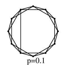
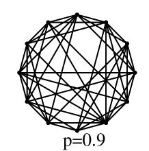
Figure 1: Small-world model with added shortcuts for different values of the adding probability $p$.

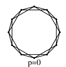
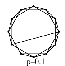
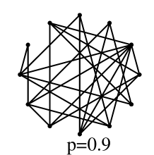
Figure 2: Small-world model with rewiring for different values of the rewiring probability $p$.

Since small-world graphs were proposed as models for complex networks [10] and  [11], most contributions in the area of complex networks focus essentially on connectivity parameters such as the degree distribution, the clustering coefficient or the shortest path length between two nodes (see e.g. [12]) . In spite of its arguable relevance — particularly where communication networks are concerned — the capacity of small-world networks has, to the best of our knowledge, not yet been studied in any depth by the scientific community. The main goal of this paper is thus to provide a preliminary characterization of the capacity of small-world networks from the point of view of network information flow.

I-B Related Work

Although the capacity of networks (described by general weighted graphs) supporting multiple communicating parties is largely unknown, progress has recently been reported in several relevant instances of this problem. In the case where the network has one or more independent sources of information but only one sink, it is known that routing offers an optimal solution for transporting messages [13] — in this case the transmitted information behaves like water in pipes and the capacity can be obtained by classical network flow methods. Specifically, the capacity of the network follows from the well-known Ford-Fulkerson max-flow min-cut theorem [14], which asserts that the maximal amount of a flow (provided by the network) is equal to the capacity of a minimal cut, i.e. a nontrivial partition of the graph node set $V$ into two parts such that the sum of the capacities of the edges connecting the two parts (the cut capacity) is minimum. In [15] it was shown that network flow methods also yield the capacity for networks with multiple correlated sources and one sink.

The case of general multicast networks, in which a single source broadcasts a number of messages to a set of sinks, is considered in [16], where it is shown that applying coding operations at intermediate nodes (i.e. network coding) is necessary to achieve the max-flow/min-cut bound of the network. In other words, if $k$ messages are to be sent then the minimum cut between the source and each sink must be of size at least $k$. A converse proof for this problem, known as the network information flow problem, was provided by [17], whereas linear network codes were proposed and discussed in [18] and [19]. Max-flow min-cut capacity bounds for Erdös-Rényi graphs and random geometric graphs were presented in [20].

Another problem in which network flow techniques have been found useful is that of finding the maximum stable throughput in certain networks. In this problem, posed by Gupta and Kumar in [21], it is sought to determine the maximum rate at which nodes can inject bits into a network, while keeping the system stable. This problem was reformulated in [22] as a multi-commodity flow problem, for which tight bounds were obtained using elementary counting techniques.

Since the seminal work of [10], key properties of small-world networks, such as clustering coefficient, characteristic path length, and node degree distribution, have been studied by several authors (see e.g. [23] and references therein). The combination of strong local connectivity and long-range shortcut links renders small-world topologies potentially attractive in the context of communication networks, either to increase their capacity or simplify certain tasks. Recent examples include resource discovery in wireless networks [24], design of heterogeneous networks  [25, 26], and peer-to-peer communications [27].

When applying small-world principles to communication networks, we would like not only that short paths exist between any pairs of nodes, but also that such paths can easily be found using merely local information. In  [28] it was shown that this navigability property, which is key to the existence of effective distributed routing algorithms, is lacking in the small-world models of  [10] and  [11]. The alternative navigable model presented in [28] consists of a grid to which shortcuts are added not uniformly but according to a harmonic distribution, such that the number of outgoing links per node is fixed and the link probability depends on the distance between the nodes. For this class of small-world networks a greedy routing algorithm, in which a message is sent through the outgoing link that takes it closest to the destination, was shown to be effective, thus opening the door towards a capacity-attaining solution.

I-C Our Contributions

We provide a set of upper and lower bounds for the max-flow min-cut capacity of several classes of small-world networks, including navigable topologies, for which highly efficient distributed routing algorithms are known to exist and distributed network coding strategies are likely to be found. Our main contributions are as follows:

• Capacity Bounds on Small-World Networks with Added Shortcuts: We prove a high concentration result which gives upper and lower bounds on the capacity of a small-world with shortcuts of probability $p$, thus describing the capacity growth due to the addition of random edges.

• Rewiring does not alter the Capacity: We construct assymptotically tight upper and lower bounds for the capacity of small-worlds with rewiring and prove that, with high probability, capacity will not change when the edges are altered in a random fashion.

• Capacity Bounds for Kleinberg Networks: We construct upper and lower bounds for the max-flow min-cut capacity of navigable small-world networks derived from a square lattice and illustrate how the choice of connectivity parameters affects communication.

• Capacity Bounds for Navigable Small-World Networks on Ring Lattices: Arguing that the corners present in the aforementioned Kleinberg networks introduce undesirable artefacts in the computation of the capacity, we define a navigable small world network based on a ring lattice, prove its navigability and derive a high-concentration result for the capacity of this instance, as well.

The rest of the paper is organized as follows. Section II establishes some notation and offers precise definitions for the small-world models of interest in this work. Our main results are stated and proved in Sections III and IV, for classical and navigable networks, respectively. The paper concludes with Section V.

II Classes of Small-World Networks

In this section, we give rigorous definitions for the classes of small-world networks under consideration. First, we require a precise notion of distance in a ring.

Definition 1

Consider a set of $n$ nodes connected by edges that form a ring (see Fig. 3, left plot). The ring distance between two nodes is defined as the minimum number of hops from one node to the other. If we number the nodes in clockwise direction, starting from any node, then the ring distance between nodes $i$ and $j$ is given by $d(i,j)=min\{|i-j|,n+i-j,n-|i-j|\}.$

For simplicity, we refer to $d(i,j)$ as the distance between $i$ and $j$. Next, we define a $k$-connected ring lattice.

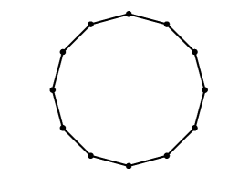
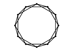
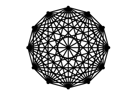
Figure 3: Illustration of a k-connected ring lattice: from left to right $k=2,4,12$.

The ring lattice that serves as basis for some of the small-world models described next, can be defined as follows.

Definition 2

A $k$-connected ring lattice (see Fig. 3) is a graph $L=(V_{L},E_{L})$ with nodes $V_{L}$ and edges $E_{L}$, in which all nodes in $V_{L}$ are placed on a ring and are connected to all the nodes within distance $\frac{k}{2}$.

Notice that in a $k$-connected ring lattice, all the nodes have degree $k$. We are now ready to define the targeted small-world models.

Definition 3 (Small-World Network with Shortcuts [11], see Fig. 1)

Consider a $k$-connected ring lattice $L=(V_{L},E_{L})$ and let $E_{C}$ be the set of all possible edges between nodes in $V_{L}$. To obtain a small-world network with shortcuts, we add to the ring lattice $L$ each edge $e\in E_{C}\backslash E_{L}$ with probability $p$.

Definition 4 (Small-World Network with Rewiring [10], see Fig. 2)

To obtain a small-world network with rewiring, we use the following procedure. Consider a $k$-connected ring lattice $L=(V_{L},E_{L})$ and choose a node, say node $u$, and the edge that connects it to its nearest neighbor in a clockwise sense. With probability $p$, reconnect this edge to a node chosen uniformly at random over the set of nodes $\left\{v\in V_{L}:(u,v)\notin E_{L}\right\}$. Repeat this process by moving around the ring in clockwise direction, considering each node in turn until one lap is completed. Next, consider the edges that connect nodes to their second-nearest neighbors clockwise. As before, randomly rewire each of these edges with probability $p$, and continue this process, circulating around the ring and proceeding outward to more distant neighbors after each lap, until each edge in the original lattice has been considered once.

Definition 5 (Kleinberg Network [28], see Fig. 4)

We begin from a two-dimensional grid and a set of nodes that are identified with the set of lattice points in an $n\times n$ square, $\{(x,y):x\in\{1,2,...,n\},y\in\{1,2,...,n\}\}$, and we define the lattice distance between two nodes $(x_{1},x_{2})$ and $(y_{1},y_{2})$ to be the number of lattice steps (or hops) separating them: $d(x,y)=|y_{1}-x_{1}|+|y_{2}-x_{2}|$. For a constant $h\geq 1$, the node $(u_{1},u_{2})$ ($\forall u_{1},u_{2}\in\left\{1,...,n\right\}$) is connected to every other node within lattice distance $h$ (we denote the set of this initial edges as $E_{L}$). For universal constants $q\geq 0$ and $r\geq 0$, we also construct edges from $u$ to $q$ other nodes using random trials; the $i^{th}$ edge from $u$ has endpoint $v$ with probability proportional to $d(u,v)^{-r}$. To ensure a valid probability distribution, consider the set of nodes that are not connected with $u$ in the initial lattice, $N_{u}=\{w:d(u,w)>h\}$, and divide $d(u,v)^{-r}$ by the appropriate normalizing constant $s(u)=\sum_{w\in N_{u}}[d(u,w)]^{-r}.$

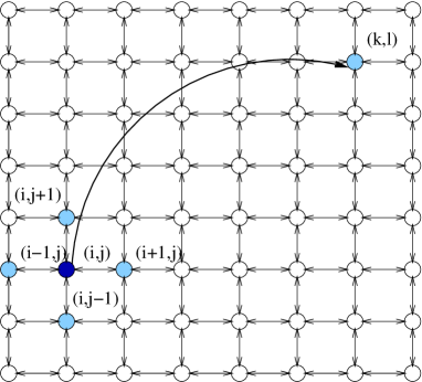
Figure 4: Kleinberg network. Each node is directly connected to all neighbors within $h$ hops, and also to $q$ more distant nodes through so called shortcuts. In the shown example, where $h=q=1$, lightly shaded circles represent the nodes that are directly connected to node $(i,j)$, i.e. the four direct neighbors of $(i,j)$ and one additional node $(k,l)$ connected by a shortcut.

In the next section, we will see that this model exhibits unexpected effects related to the corners of the chosen base lattice. Motivated by this observation, we construct a somewhat different model, which uses a ring lattice but still keeps the key relationship between shortcut probability and node distance that assures the navigability of the model (as proven in the appendix).

Definition 6 (Navigable Small-World Ring)

Consider a $k$-connected ring lattice. For universal constants $q\geq 0$ and $r\geq 0$, we add new edges from node $i$ ($\forall i$) to $q$ other nodes randomly: each added edge has an endpoint $j$ with probability proportional to $d(i,j)^{-r}$. To ensure a valid probability distribution, consider $N_{i}=\left\{j:d(i,j)>\frac{k}{2}\right\}$ and divide $d(i,j)^{-r}$ by the appropriate normalizing constant $s_{i}=\sum_{j\in N_{i}}d(i,j)^{-r}$.

III Capacity Results for Small-World Networks

In Section I-B, we argued that the max-flow min-cut capacity provides the fundamental limit of communication for various relevant network scenarios. Motivated by this observation, we will now use network flow methods and random sampling techniques in graphs to derive a set of bounds for the capacity of the small-world network models presented in the previous section. Although all of the models discussed in this section are based on ring lattices, it is worth pointing out that the methodology presented next can be equally applied to other classes of base lattices.

III-A Preliminaries

We start by introducing some necessary mathematical tools. Let $G$ be an undirected graph, representing a communication network, with edges of unitary weight. In the spirit of the max-flow min-cut theorem of Ford and Fulkerson [14], we will refer to the global minimum cut of $G$ as the max-flow min-cut capacity (or simply the capacity) of the graph.

Let $G_{s}$ be the graph obtained by sampling on $G$, such that each edge $e$ has sampling probability $p_{e}$. From $G$ and $G_{s}$, we obtain $G_{w}$ by assigning to each edge $e$ the weight $p_{e}$, i.e. $w(e)=p_{e},\forall e$. We denote the capacity of $G_{s}$ and $G_{w}$ by $c_{s}$ and $c_{w}$, respectively. It is helpful to view a cut in $G_{s}$ as a sum of Bernoulli experiences, whose outcome determines if an edge $e$ connecting the two sides of the cut belongs to $G_{s}$ or not. It is not difficult to see that the value of a cut in $G_{w}$ is the expected value of the same cut in $G_{s}$. The next theorem gives a characterization of how close a cut in $G_{s}$ will be with respect to its expected value.

Theorem 1 (From [29])

Let $\epsilon=\sqrt{2(d+2)\ln(n)/c_{w}}$. Then, with probability $1-O(1/n^{d})$, every cut in $G_{s}$ has value between $(1-\epsilon)$ and $(1+\epsilon)$ times its expected value.

Notice that although $d$ is a free parameter, there is a strict relationship between the value of $d$ and the value of $\epsilon$. In other words, the proximity to the expected value of the cut is intertwined with how close the probability is to one. Theorem 1 yields also the following useful property.

Corollary 1

Let $\epsilon=\sqrt{2(d+2)\ln(n)/c_{w}}$. Then, with high probability, the value of $c_{s}$ lies between $(1-\epsilon)c_{w}$ and $(1+\epsilon)c_{w}$.

Before using the previous random sampling results to determine bounds for the capacities of small-world models, we prove another useful lemma.

Lemma 1

Let $L=(V_{L},E_{L})$ be a $k$-connected ring lattice and let $G=(V_{L},E)$ be a fully connected graph (without self-lops), in which edges $e\in E_{L}$ have weight $w_{1}\geq 0$ and edges $f\notin E_{L}$ have weight $w_{2}\geq 0$. Then, the global minimum cut in $G$ is $kw_{1}+(n-1-k)w_{2}$.

Proof:

We start by splitting $G$ into two subgraphs: a $k$-connected ring lattice $L$ with weights $w_{1}$ and a graph $F$ with nodes $V_{L}$ and all remaining edges of weight $w_{2}$. Clearly, the value of a cut in $G$ is the sum of the values of the same cut in $L$ and in $F$. Moreover, both in $L$ and in $F$, the global minimum cut is a cut in which one of the partitions consists of one node (any other partition increases the number of outgoing edges). Since each node in $L$ has $k$ edges of weight $w_{1}$ and each node in $F$ has the remaining $n-1-k$ edges of weight $w_{2}$, the result follows. ∎

III-B Capacity Bounds for Small-World Networks with Added Shortcuts

With this set of tools, we are ready to state and prove our first main result.

Theorem 2

With high probability, the value of the capacity of a small-world network with added shortcuts lies between $(1-\epsilon)c_{w}$ and $(1+\epsilon)c_{w}$, with $\epsilon=\sqrt{2(d+2)\ln(n)/c_{w}}$ and $c_{w}=k+(n-1-k)p.$

Proof:

Let $G_{w}$ be a fully connected graph with $n$ nodes and with the edge weights (or equivalently, the sampling probabilities) defined as follows:

• The weight of the edges in the initial lattice of a small-world network with added shortcuts is one (because they are not removed);

• The weight of the remaining edges is $p$, (i.e. the probability that an edge is added).

Notice that $G_{w}$ is a graph in the conditions of Lemma 1, with $w_{1}=1$ and $w_{2}=p$. Therefore, the global minimum cut in $G_{w}$ is $c_{w}=k+(n-1-k)p$, where $k$ is the initial number of neighbors in the lattice. Using Corollary 1, the result follows. ∎

The obtained bounds are illustrated in Fig. 5.

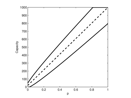
Figure 5: Bounds on the capacity of a small-world network with added shortcuts, for $n=1000$, $k=20$, and $d=1$. The dashed line represents the expected value of the capacity, and the solid lines represent the bounds. Naturally, the capacity increases with $p$, as the number of added links become larger.

III-C Capacity Bounds for Small-World Networks with Rewiring

In the previous classes of small-world networks, edges were added to a $k$-connected ring lattice (with minimum cut $k$) and clearly the capacity could only grow with $p$. The next natural step is to ask what happens when edges are not added but rewired with probability $p$, as described in Section II. Before presenting a theorem that answers this question, we will prove the following lemma.

Lemma 2

Let $G_{w}$ be a weighted, fully connected graph, whose weights correspond to the edge probabilities of a small-world network with rewiring, and let $c_{w}$ be the global minimum cut in $G_{w}$. Then, $c_{w}\geq k$.

Proof:

We start with the initial lattice edges $(l,m)\in E_{L}$, and assign the weight $1-p$ to their counterparts in $G_{w}$. In order to determine the weight of the non-initial edges that result from rewiring, consider the following events:

• $R(i,j)$: “Choose the edge $(i,j)\in E_{L}$ to be rewired”;

• $C_{i}(j,l)$: “Rewire $(i,j)\in E_{L}$ to $(i,l)\notin E_{L}$”.

Notice that ${\cal P}(R(i,j))=p,\forall(i,j)\in E_{L}$.
Let $i$ and $j$ be two non-initially connected nodes. The notation $i\leftrightarrow j$ denotes the event that the nodes $i$ and $j$ are connected. We have that

$${\cal P}(i\leftrightarrow j) = {\cal P}\left([\cup_{x=1}^{k/2}(R(i,i+x)\cap C_{i}(i+x,j))]\cup[\cup_{x=1}^{k/2}(R(j,j+x)\cap C_{j}(j+x,i))]\right)$$

$$= {\cal P}\left(\cup_{x=1}^{k/2}(R(i,i+x)\cap C_{i}(i+x,j)))+{\cal P}(\cup_{x=1}^{k/2}(R(j,j+x)\cap C_{j}(j+x,i))\right)$$

$$-{\cal P}\left([\cup_{x=1}^{k/2}(R(i,i+x)\cap C_{i}(i+x,j))]\cap[\cup_{x=1}^{k/2}(R(j,j+x)\cap C_{j}(j+x,i))]\right)$$

Because we do not consider multiple edges, we have that the events $R(i,i+x)\cap C_{i}(i+x,j)$ and $R(j,j+y)\cap C_{j}(j+y,i)$ are mutually exclusive, $\forall x,y$. Therefore,

$${\cal P}(i\leftrightarrow j) = \sum_{x=1}^{k/2}\left({\cal P}(R(i,i+x)\cap C_{i}(i+x,j))+{\cal P}(R(j,j+x)\cap C_{j}(j+x,i))\right)$$

$$= \sum_{x=1}^{k/2}\left({\cal P}(C_{i}(i+x,j)|R(i,i+x)){\cal P}(R(i,i+x))+{\cal P}(C_{j}(j+x,i)|R(j,j+x)){\cal P}(R(j,j+x))\right)$$

$$= p\cdot\left(\sum_{x=1}^{k/2}({\cal P}(C_{i}(i+x,j)|R(i,i+x))+{\cal P}(C_{j}(j+x,i)|R(j,j+x)))\right).$$

We have ${\cal P}(C_{i}(i+x,j)|R(i,i+x))=\frac{1}{m}$, where $m$ is the number of possible new connections from node $i$ when we rewired the edge $(i,i+x)$. It is possible that, occurring some rewiring or not, none of the choices to a new link is the node $i$. In this case, $m=n-k-1$. Notice that this is the highest it can get, therefore $m\leq n-k-1$. Then, we have

$${\cal P}(C_{i}(i+x,j)|R(i,i+x))\geq\frac{1}{n-k-1}.$$

Analogously, ${\cal P}(C_{j}(j+x,i)|R(j,j+x)))\geq\frac{1}{n-k-1}$. Therefore,

$${\cal P}(i\leftrightarrow j)\geq p\cdot\left(\sum_{x=1}^{k/2}\frac{2}{n-k-1}\right)=\frac{pk}{n-k-1}.$$

There are $k$ initial edges and $n-k-1$ non-initial edges in each node.

Consider a fully connected, weighted graph $F$ with the weights defined as follows: all the edges $(i,j)\notin E_{L}$ have the weight $\frac{pk}{n-k-1}$, and all the others edges $(i,j)\in E_{L}$ have the weight $1-p$. Notice that $F$ is a graph in the conditions of Lemma $1$, with $w_{1}=1-p$ and $w_{2}=\frac{pk}{n-k-1}$. Therefore,

$$c_{F}=k(1-p)+(n-k-1)\frac{pk}{n-k-1}=k.$$

Notice that, in this situation, all the weights in $F$ are a lower bound of the weights in $G_{w}$. Therefore, a cut in $F$ is a lower bound for the corresponding cut in $G_{w}$. Then, the global minimum cut in $F$ is a lower bound for all the cuts in $G_{w}$, in particulary, for $c_{w}$: $c_{w}\geq c_{F}=k$. ∎

With this lemma, we are now ready to state and prove our next result.

Theorem 3 (Rewiring does not alter capacity.)

With high probability, the capacity of a small-world network with rewiring has a value in the interval $[(1-\epsilon)k,k]$ with $\epsilon=\sqrt{2(d+2)ln(n)/k}$.

Proof:

Based on Lemma 2 and Corollary 1, we have that, with high probability, $c_{s}\geq(1-\epsilon_{w})k$, with $\epsilon_{w}=\sqrt{2(d+2)ln(n)/c_{w}}$. Now, from the fact that $c_{w}\geq k$, we have that $\epsilon=\sqrt{2(d+2)ln(n)/k}\geq\epsilon_{w}$. Then, $(1-\epsilon_{w})k\geq(1-\epsilon)k$, and the first part of the result follows.

Next, we prove by contradiction that $c_{s}\leq k$. Suppose that the proposition $c_{s}>k$ is true. Let $c_{i}$ be the cut in which one of the partitions consists of node $i$, $i=1,...,n$. Because $c_{s}$ is the global minimum cut in $G_{s}$, we have that $c_{i}>k$, $\forall i=1,...,n$. Notice that $c_{i}$ is the degree of node $i$. Then, because in the $k$-connected ring lattice all nodes have degree $k$ and all nodes in $G_{s}$ have degree greater than $k$ (because $c_{i}>k,\forall i$), we have that the number of edges in $G_{s}$ must be greater than the number of edges in the $k$-connected ring lattice. But this is clearly absurd, because in the construction of $G_{s}$, we do not add new edges to the $k$-connected ring lattice, we just rewire some of the existent edges. ∎

IV Capacity Bounds for Navigable Networks

As we argue in Section I, when considering small-world networks as communication networks, an important aspect is the ability to find short paths between any pairs of nodes, using only local information. This property guarantees that efficient distributed routing algorithms exists. Kleinberg, in his seminal work [28], proved that this navigability property is lacking in the models of Watts and Strogatz, and introduced a new model (Definition 5). Motivated by the relevance of the navigability property, we present, in this section, the capacity bounds for Kleinberg Networks and for Navigable Small-World Rings.

IV-A Capacity Bounds for Kleinberg Networks

Before proceeding with the bounds for the capacity of Kleinberg networks, we require an algorithm to calculate the normalizing constants $s(x,y)=\sum_{(i,j)\in N_{(x,y)}}[d((x,y),(i,j))]^{-r}$ for $x,y\in\{1,...n\}$. For this purpose, we note that the previous sum can be written as

$$s(x,y)=\sum\limits_{(i,j)\neq(x,y)}[d((i,j),(x,y))]^{-r}-\sum_{(i,j)\notin N_{(x,y)}}[d((i,j),(x,y))]^{-r}.$$

Clearly, the first term can be easily calculated. Thus, the challenging task is to present an algorithm that deals with the calculation of $\sum_{(i,j)\notin N_{(x,y)}}[d((i,j),(x,y))]^{-r}$. The nodes $(i,j)\notin N_{(x,y)}$ are the nodes initially connected to node $(x,y)$, i.e., the nodes at a distance $t\leq h$ from node $(x,y)$. It is not difficult to see that the nodes at a distance $t$ from node $(x,y)$ are the nodes in the square line formed by the nodes $(x-t,y)$, $(x+t,y)$, $(x,y+t)$ and $(x,y-t)$. Then, we could just look at nodes in the square formed by the nodes $(x-h,y)$, $(x+h,y)$, $(x,y+h)$ and $(x,y-h)$ and sum all the corresponding distances to node $(x,y)$. A corner effect occurs when when this square lies outside the base lattice. Assume that we start by calculating the distances to the nodes in line $y+i$, with $i\geq 0$.

TABLE I: Algorithm for computing normalizing constants

Algorithm 1

$\ \ z=[0]_{n\times n}$
$\ \ for\>i=0:min\{h,n-y\}$
$\ \ \ \ \ \ for\>j=0:min\{h-i,n-x\}$
$\ \ \ \ \ \ \ \ \ \ z(x+j,y+i)=(i+j)^{-r}$
$\ \ \ \ \ \ for\>j=1:min\{h-i,x-1\}$
$\ \ \ \ \ \ \ \ \ \ z(x-j,y+i)=(i+j)^{-r}$
$\ \ for\>i=1:min\{h,y-1\}$
$\ \ \ \ \ \ for\>j=0:min\{h-i,n-x\}$
$\ \ \ \ \ \ \ \ \ \ z(x+j,y-i)=(i+j)^{-r}$
$\ \ \ \ \ \ for\>j=1:min\{h-i,h-(m_{1}-i),x-1\}$
$\ \ \ \ \ \ \ \ \ \ z(x-j,y-i)=(i+j)^{-r}$
$\ \ z(x,y)=0$
$\ \ z=\sum_{i=1}^{n}\sum_{j=1}^{n}z(i,j)$
$\ \ s(x,y)=\sum_{(i,j)\neq(x,y)}(|i-x|+|j-y|)^{-r}-z$

To avoid calculating extra distances (i.e., distances of nodes that are out of the grid), we must make sure that this line verifies $y+i\leq n$ and also $y+i\leq h$. For this reason, $i$ must vary according to $i\in\{0\dots\min\{h,n-y\}\}$. Now, in each line $y+i$, we first look at the nodes in the right side of $(x,y)$, i.e., we calculate the distances of the nodes $(x+j,y+i)$, with $j\geq 0$. Now, notice that in the line $y$, we have $h$ points on the right side of $(x,y)$ that are in the square (regardless of whether they are in the grid). Because the distance is the minimum number of steps in the grid, we have that in line $y+i$ there are $h-i$ points at the right side of $(x,y)$ that are inside the square. This way, $j$ must be vary according to $j\in\{0\dots\min\{h-i,n-x\}\}$. Now, when looking at the nodes at the left side (i.e., the nodes $(x-j,y+i)$, with $i\geq 1$), the idea is the same. The only difference is that, in this case, the variation for $j$ is $j\in\{1\dots\min\{h-i,x-1\}\}$. Then, we proceed analogously for the lines below $(x,y)$, i.e., the lines $y-i$, with $i\in\{1\dots\min\{h,y-1\}\}$. This algorithm is summarized in Table I. The matrix $z$ is a buffer for the distances, i.e., $z(u_{1},u_{2})=d((x,y),(u_{1},u_{2}))$. We impose $z(x,y)=0$, because $d((x,y),(x,y))^{-r}$ is also calculated in this procedure.

The following quantities will be instrumental towards characterizing the capacity:

$$M = \max\left\{\frac{h(h+3)}{2}+q,(1-\epsilon)c_{w}\right\}$$

$$\epsilon = \sqrt{2(d+2)\ln(n^{2})/c_{w}}$$

$$c_{w} = \frac{h(h+3)}{2}+\sum_{x=1}^{h+1}\sum_{y=h+2-x}^{n}f(x,y)+\sum_{x=h+2}^{n}\sum_{y=1}^{n}f(x,y)$$ (1)

$$f(x,y) = q\cdot(g_{(x,y)}(1,1)+g_{(1,1)}(x,y))$$

$$g_{(x,y)}(a,b) = \left(1-\frac{(x+y-2)^{-r}}{s(a,b)}\right)^{q-1}\cdot\frac{(x+y-2)^{-r}}{s(a,b)}$$

$$s(1,1) = \sum_{i=h+1}^{n-1}(i+1)\cdot i^{-r}+\sum_{i=0}^{n-2}(n-1-i)\cdot(n+i)^{-r}.$$

Recall that $s(x,y)$ can be calculated using Algorithm 1. The proof of the capacity will rely heavily on the following lemma.

Lemma 3

Let $G_{w}$ be the weighted graph associated with a Kleinberg network, and $c_{w}$ be the global minimum cut in $G_{w}$. Then, for $h<n-1$, $c_{w}$ is given by (1).

Proof:

All the edges $e\in E_{L}$ have weight $1$ (because they are never removed), all nodes in $G_{w}$ have degree $n^{2}-1$, and the weights of these edges depend only on the distance between the nodes they connect. Therefore, the global minimum cut in $G_{w}$ must be a cut in which one of the partitions consists of a single node. Because the weight of an edge in $G_{w}$ decreases with the distance between the nodes that it connects, the global minimum cut in $G_{w}$ must be a cut in which one of the partitions consists of a single node that maximizes the distance to other nodes. Therefore, because a corner node has more nodes at a greater distance than the other nodes and has also a smaller number of nodes to which it is connected, $c_{w}$ must be a cut in which one of the partitions consists of a corner node: $(1,1),(1,n),(n,1)$ or $(n,n)$.

Assume, without loss of generality, that $c_{w}$ is the cut in which one of the partitions consists of node $(1,1)$. Let $w(u,v)$ be the weight of the edge connecting the nodes $u$ and $v$. This way, $c_{w}=\sum_{u\neq(1,1)}w((1,1),u)$. Now, we must count how many edges connecting node $(1,1)$ are in $E_{L}$, therefore, having weight $1$. For this, we define an auxiliary way to numerate diagonals: $\{(1,1)\}$ is the diagonal $0$, $\{(1,2),(2,1)\}$ is diagonal 1, and so on (see Figure 6).

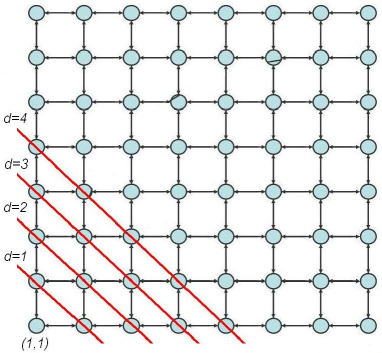
Figure 6: Numeration of the diagonals of a square lattice.

It is not difficult to see that the nodes in the $i^{th}$ diagonal have a distance $i$ to node $(1,1)$, $i\in\{1,...,2(n-1)\}$. Now, for $i\leq n-1$, there are $i+1$ nodes in the $i^{th}$ diagonal and, for $i=n+j$ with $j\in\{0,...,n-2\}$, there are $n-1-j$ nodes in the $i^{th}$ diagonal. Then, there are $\sum_{i=1}^{h}i+1=h(h+3)/2$ nodes initially connected to node $(1,1)$ (again, with $h<n-1$), then there are $h(h+3)/2$ edges with weight 1. Therefore, we have that:

$$c_{w}=\frac{h(h+3)}{2}+\sum_{x=1}^{h+1}\sum_{y=h+2-x}^{n}w((1,1),(x,y))+\sum_{x=h+2}^{n}\sum_{y=1}^{n}w((1,1),(x,y)).$$

Next, we determine the weights, $w(u,v)$. Consider two nodes that are not connected initially, $u=(u_{1},u_{2})$ and $v=(v_{1},v_{2})$, and the edge $(u,v)$. This edge can be added in two different trials: one for node $u$ and another one for node $v$. Because we do not consider multiple edges, these can be viewed as two mutually exclusive trials. Therefore, the weight of this edge is the sum of the probabilities of adding this edge when considering node $u$ and when considering node $v$. Let us focus on node $u$. The trial “add edge $(u,v)$” follows a Binomial distribution, with $q$ Bernoulli experiences, with success probability

$$a_{u}(v)=\frac{d(u,v)^{-r}}{s(u)}=\frac{(|u_{1}-v_{1}|+|u_{2}-v_{2}|)^{-r}}{s(u)}.$$

Therefore, the probability of adding the edge $(u,v)$, when considering node $u$, is $q\cdot(1-a_{u}(v))^{q-1}\cdot a_{u}(v)$. Therefore, the weight of the edge $((u_{1},u_{2}),(v_{1},v_{2}))$ is

$$w(u,v)=q\cdot(1-a_{u}(v))^{q-1}\cdot a_{u}(v)+q\cdot(1-a_{v}(u))^{q-1}\cdot a_{v}(u).$$

As we have seen, the global minimum cut in $G_{w}$ is the cut in which one of the partitions consists of node $(1,1)$. We have that, if $(x,y)$ is a node of the grid, $x\geq 1$ and $y\geq 1$. Then, $d((1,1),(x,y))=|x-1|+|y-1|=x+y-2$. Therefore, $a_{(1,1)}(x,y)=\frac{x+y-2}{s(1,1)}$ and $a_{(x,y)}(1,1)=\frac{x+y-2}{s(x,y)}$. Now, observing that we can calculate $s(1,1)$ as

$$s(1,1)=\sum_{i=h+1}^{n-1}(i+1)\cdot i^{-r}+\sum_{i=0}^{n-2}(n-1-i)\cdot(n+i)^{-r}$$

and using expression (1) for $c_{w}$, the result follows. ∎

We are now ready to state our main result.

Theorem 4

For $h<n-1$ the capacity of a Kleinberg small-world network graph lies, with high probability, in the interval $\left[M,(1+\epsilon)c_{w}\right]$.

Proof:

Using Lemma 3 and Corollary 1, we have that, with high probability, $c_{s}\in\left[(1-\epsilon)c_{w},(1+\epsilon)c_{w}\right].$ A tighter lower bound can be obtained for $c_{s}$ as follows. Each node has a number of initial edges, determined by $h$, and $q$ additional shortcut edges. The nodes with less initial edges are obviously the corner nodes, which exhibit $\frac{h(h+3)}{2}$ initial connections. Therefore, we have that $c_{s}\geq\frac{h(h+3)}{2}+q,$ and the result follows. ∎

The bounds of Theorem 4 are illustrated in Fig. 7.

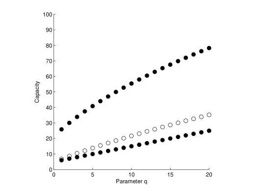
Figure 7: Bounds for the capacity of Kleinberg small-world network for $n=80$ (i.e. 1600 nodes), $h=2$, $r=2$ e $d=1$, and different values of the shortcut parameter $q$. The white dots represent the expected value of the capacity and the dark dots represent the bounds computed according to Theorem 4.

IV-B Capacity Bounds for Navigable Small-World Rings

As we have seen, Kleinberg’s model exhibits corner’s effects in terms of capacity. With the goal of overcoming this problem, we defined a new class of small-world networks, the navigable small-world ring (see Definition 6 in Section II), whose navigability is proven in the appendix. Now we study the capacity of this class of networks by proving the following result.

Theorem 5

With high probability, the capacity of the navigable small-world ring has a value in the interval $\left[\max\left\{k,(1-\epsilon)c_{w})\right\},(1+\epsilon)c_{w})\right]$, with $\epsilon=\sqrt{2(d+2)\ln(n)/c_{w}}$ and

$$c_{w}=k+2^{rq+1}s^{-q}q(1+a_{n})(n-a_{n})^{-r}\left(2^{-r}s-(n-a_{n})^{-r}\right)^{q-1}+4qs^{-q}\cdot\sum_{i=\frac{k}{2}+1}^{\frac{n-a_{n}}{2}-1}i^{-r}\left(s-i^{-r}\right)^{q-1}$$

with $s=(1+a_{n})\cdot\left(\frac{n-a_{n}}{2}\right)^{-r}+2\cdot\sum\limits_{i=\frac{k}{2}+1}^{\frac{n-a_{n}}{2}-1}i^{-r}$, where $a_{n}=\frac{1-(-1)^{n}}{2}$.

Proof:

Consider the fully connected graph $G_{w}=(V_{L},E)$ associated to the navigable small-world graph. The task is to determine the weights of the edges of $G_{w}$. The edges $e\in E_{L}$ have weight $1$, because we never remove them. Now, notice that the ring distance between two nodes does not depend on which node is numbered first. It is therefore correct to state that all the nodes have the same number of nodes at a distance $d$. Therefore, we have that the normalizing constants are equal, for all nodes: $s_{i}=s_{j},\forall i,j$. Let $s=s_{i}$. We also have that the weight of each edge only depends on the distance between the nodes that it connects. Therefore, it is sufficient to determine the weights of the edges of a single node, say node $1$.

First, we must compute the normalizing constant $s$. We must distinguish between two different situations: even $n$ or odd $n$. If $n$ is even, it is not difficult to see that there is a single node that maximizes the distance to node $1$. That node is node $\frac{n}{2}+1$, and we have that $d\left(1,\frac{n}{2}+1\right)=\frac{n}{2}$. For distances $d<\frac{n}{2}$, there are two nodes at distance $d$ to node $1$. Therefore, if $n$ is even, we have that

$$s=\left(\frac{n}{2}\right)^{-r}+2\cdot\sum_{i=\frac{k}{2}+1}^{\frac{n}{2}-1}i^{-r}.$$

When $n$ is odd, it is also easy to see that there are two nodes that maximize the distance to node $1$: nodes $\frac{n+1}{2}$ and $\frac{n+3}{2}$, with the maximum distance being $\frac{n-1}{2}$. Therefore, if $n$ is odd, we have that

$$s=2\cdot\sum_{i=\frac{k}{2}+1}^{\frac{n-1}{2}}i^{-r}.$$

Now, just notice that $a_{n}=\frac{1-(-1)^{n}}{2}$ is equal to $0$ if $n$ is even, and it is equal to $1$ if $n$ is odd. Therefore,

$$s=(1+a_{n})\cdot\left(\frac{n-a_{n}}{2}\right)^{-r}+2\cdot\sum_{i=\frac{k}{2}+1}^{\frac{n-a_{n}}{2}-1}i^{-r}.$$

Consider a node that is not initially connected to node $1$, say node $i$. The edge $(1,i)$ can be added in two different trials: one for node $1$ and another for node $i$. Because we do not consider multiple edges, these two trials are mutually exclusive. Therefore, the weight of the edge $(1,i)$ is the sum of the probabilities of adding this edge when looking at node $1$ and when looking at node $i$. Because the normalizing constant is the same for all nodes, these two probabilities are equal. This way, let us focus on node $1$. The trial “add edge $(1,i)$” follows a Binomial distribution, with $q$ Bernoulli experiences and with success probability $p=\frac{d(1,i)^{-r}}{s}$. Therefore, the probability of adding edge $(1,i)$ when considering node $1$ is $qp\cdot(1-p)^{q-1}$. Therefore, the weight of the edge $(1,i)$ is

$$w(1,i)=2q\cdot\frac{d(1,i)^{-r}}{s}\cdot\left(1-\frac{d(1,i)^{-r}}{s}\right)^{q-1}.$$

We have seen that all the nodes have the same number of nodes at a distance $d$. We also have that all the edges in the ring lattice have unitary weight. Based on these two observations and the fact that $G_{w}$ is a fully connected graph, it is clear that the global minimum cut in $G_{w}$, denoted $c_{w}$, is a cut in which one of the partitions consists of a single node, say node $1$. Thus, we may write

$$c_{w} = k+\sum_{i\in N_{1}}w(1,i)$$

$$= k+2(1+a_{n})q\frac{\left(\frac{n-a_{n}}{2}\right)^{-r}}{s}\left(1-\frac{\left(\frac{n-a_{n}}{2}\right)^{-r}}{s}\right)^{q-1}+2\cdot\sum_{i=\frac{k}{2}+1}^{\frac{n-a_{n}}{2}-1}2q\frac{i^{-r}}{s}\left(1-\frac{i^{-r}}{s}\right)^{q-1}$$

$$= k+2^{rq+1}s^{-q}q(1+a_{n})(n-a_{n})^{-r}\left(2^{-r}s-(n-a_{n})^{-r}\right)^{q-1}+4qs^{-q}\cdot\sum_{i=\frac{k}{2}+1}^{\frac{n-a_{n}}{2}-1}i^{-r}\left(s-i^{-r}\right)^{q-1}$$

Now, using Corollary 1 and noticing that, because we only add new edges to the initial $k$-connected ring lattice and this lattice has capacity $k$, the capacity can only be greater than $k$, we obtain the desired bounds. ∎

The result is illustrated in Fig. 8.

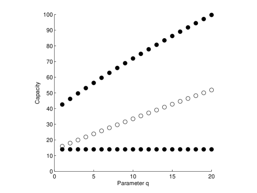
Figure 8: Bounds for the capacity of a navigable small-world ring for $n=1600$, $k=14$, $r=1$ e $d=1$, and different values of the shortcut parameter $q$. The white dots represent the expected value of the capacity and the dark dots represent the bounds computed according to Theorem 5.

V Concluding Remarks

We studied the max-flow min-cut capacity of four fundamental classes of small-world networks. Using classical network flow arguments and concentration results from random sampling in graphs, we provided bounds for both standard and navigable small-world networks with added shortcuts, and also for Kleinberg’s model. In addition, we presented a tight result for small-world networks with rewiring, which permits the following interpretation: With high probability, rewiring does not alter the capacity of the network. This observation is not obvious, because we can easily find ways to rewire the ring lattice in order to obtain, for instance, a bottleneck. But, according to the previous results, such instances occur with very low probability.

In [28], Kleinberg explains that, in order to obtain a probability distribution, $d((u_{1},u_{2}),(v_{1},v_{2}))^{-r}$ should be divided by $\sum_{(v_{1},v_{2})\neq(u_{1},u_{2})}[d((u_{1},u_{2}),(v_{1},v_{2}))]^{-r}.$ As we have shown, the previous expression is not an accurate normalizing constant for our work, because we consider undirected edges. Then, the candidates for new connections from node $(u_{1},u_{2})$ are not all the nodes of the base lattice, but only those nodes that are initially not connected to node $(u_{1},u_{2})$.

Possible directions for future work include tighter capacity results, extensions to other classes of small-world networks (e.g. weighted models and those used in peer-to-peer networks [27]), and understanding if and how small-world topologies can be exploited in the design of capacity-attaining network codes and distributed network coding algorithms. At a more conceptual level, we are intrigued by the possibility that the notion of capacity may help us answer a very central question: why small-world topologies are ubiquitous in real-world networks.

Proof of Navigability of the Small-World Ring

As we have discussed in Section I, in the context of communication networks, we would like that not only short paths exist between any pair of nodes, but also that paths can easily be found using only local information. Kleinberg, in [28], showed that this navigability property is absent in the initial models of small-world networks, from Watts and Strogatz. This way, Kleinberg felt the need to introduce a new model, the model defined in Definition 5, that captures this fundamental property. In his work, Kleinberg uses the idea of a decentralized algorithm to study the navigability property.

Definition 7

Consider a graph $G$ with an underlying metric $\delta_{G}$. A decentralized algorithm in $G$ is an algorithm with the goal of sending a message from a source to a destination, with the knowledge, at each step, of the underlying metric, the position of the destination, and the contacts of the current message holder and of all the nodes seen so far.

Definition 8

A greedy decentralized algorithm is a decentralized algorithm operating greedily: at each step, it sends the message to the contact of the current message holder that is closer (in the sense of the underlying metric) to destination.

In [28], Kleinberg proved that the models presented by Watts and Strogatz do not admit efficient decentralized algorithms, in constrast with his model:

Theorem 6 (From [28])

For $r=2$, there is a constant $\alpha_{2}$, independent of $n$, so that the expected delivery time of a greedy decentralized algorithm in a Kleinberg network is at most $\alpha_{2}\cdot\log^{2}(n)$.

Theorem 7 (From [28])

1. Let $0\leq r<2$. There is a constant $\alpha_{r}$, depending on $p$, $q$, $r$, but independent of $n$, so that the expected delivery time of any decentralized algorithm in a Kleinberg network is at least $\alpha_{r}\cdot n^{(2-r)/3}$.

2. Let $r>2$. There is a constant $\alpha_{r}$, depending on $p$, $q$, $r$, but independent of $n$, so that the expected delivery time of any decentralized algorithm in a Kleinberg network is at least $\alpha_{r}\cdot n^{(r-2)/(r-1)}$.

Theorem 6 shows that, in fact, a Kleinberg network is navigable, while Theorem 7 shows that the models from Watts and Strogatz are not navigable, because this is the case when we consider uniformly chosen shortcuts, therefore corresponding to $r=0$.

The next theorem shows that a navigable small-world ring is, indeed, navigable, in the sense that the expected delivery time of a decentralized algorithm is logarithmic. The proof is essentially based on the proof of Theorem 6 presented by Kleinberg.

Theorem 8

For $r=1$, the expected delivery time of a greedy decentralized algorithm in a navigable small-world ring is at most $\frac{\ln^{2}(2n)}{\ln(2)}$.

Proof:

First, we need to show that $\sum_{u\notin N_{v}}d(u,v)^{-1}$ is uniformly bounded. For even $n$, it is not difficult to see that there is a single node that maximizes the distance to node $1$. That node is node $\frac{n}{2}+1$, and we have that $d\left(1,\frac{n}{2}+1\right)=\frac{n}{2}$. For distances $d<\frac{n}{2}$, there are two nodes at distance $d$ to node $1$. Therefore, if $n$ is even, we have that

$$\sum_{u\notin N_{v}}d(u,v)^{-1}=\left(\frac{n}{2}\right)^{-1}+2\cdot\sum_{i=\frac{k}{2}+1}^{\frac{n}{2}-1}i^{-1}\leq 2\cdot\sum_{i=\frac{k}{2}+1}^{\frac{n}{2}}i^{-1}.$$

When $n$ is odd, it is also easy to see that there are two nodes that maximize the distance to node $1$: nodes $\frac{n+1}{2}$ and $\frac{n+3}{2}$, with the maximum distance being $\frac{n-1}{2}$. Therefore, if $n$ is odd, we have that

$$\sum_{u\notin N_{v}}d(u,v)^{-1}=2\cdot\sum_{i=\frac{k}{2}+1}^{\frac{n-1}{2}}i^{-1}.$$

Therefore, we have that $\forall n\in$$\mathbb{N}$,

$$\sum_{u\notin N_{v}}d(u,v)^{-1} \leq 2\cdot\sum_{i=\frac{k}{2}+1}^{\left\lfloor\frac{n-1}{2}\right\rfloor}i^{-1}$$

$$\leq 2\cdot\sum_{i=1}^{\left\lfloor\frac{n-1}{2}\right\rfloor}i^{-1}$$

$$\leq 2+2\ln\left(\frac{n}{2}\right)$$

$$\leq 2\ln(2n).$$

For $j>0$, we say that the decentralized algorithm is in phase $j$ if the distance between the current message holder and the destination is $d$ such that $2^{j}<d\leq 2^{j+1}$. We say that the algorithm is in phase $0$ if the distance between the current message holder and the destination is at most $2$. Because the maximum distance in the ring-lattice is at most $\frac{n}{2}$, we have that $j\leq\log\left(\frac{n}{2}\right)$.

Now, suppose that we are in phase $j$ and the current message holder is node $u$. The task is to determine the probability of phase $j$ ending in this step. Let $B_{j}$ be the set of nodes within lattice distance $2^{j}$ of the destination. Phase $j$ ending in this step means that $u$ chooses a long-range contact $v\in B_{j}$. Each node $v\in B_{j}$ as probability of being chosen as long-range contact of $u$ at least

$$\frac{\left(2^{j}\right)^{-1}}{\sum_{v\notin N_{u}}d(u,v)^{-1}}\geq\frac{1}{2^{j+1}\cdot\ln(2n)}.$$

We have that the number of nodes in $B_{j}$, denoted by $|B_{j}|$, verifies

$$|B_{j}|=1+2\cdot\sum_{i=1}^{2^{j}}i\geq 2^{2j}.$$

Therefore, with $A$ denoting the event “Phase $j$ ends in this step”, we have that

$${\cal P}(A)\geq\frac{2^{2j}}{2^{j+1}\cdot\ln(2n)}=\frac{2^{j-1}}{\ln(2n)}\geq\frac{1}{\ln(2n)}.$$

Let $N_{j}$ be the number of steps spent in phase $j$. Now, we must compute the expected value of $N_{j}$. Notice that the maximum number of steps spent in phase $j$ is the number of nodes at distance of the destination $d$ such that $2^{j}<d\leq 2^{j+1}$, which is

$$m = 2\cdot\sum_{i=2^{j}}^{2^{j+1}-1}i$$

$$= 2\cdot\left(\sum_{i=1}^{2^{j+1}-1}i-\sum_{i=1}^{2^{j}-1}i\right)$$

$$= 2^{j+1}(2^{j+1}-1)-2^{j}(2^{j}-1)$$

$$\leq 2^{2j+2}.$$

Therefore, the expected value of $N_{j}$ verifies the following:

$$E\left(N_{j}\right) = \sum_{i=1}^{m}{\cal P}(N_{j}\geq i)$$

$$\leq \sum_{i=1}^{2^{2j+2}}{\cal P}(N_{j}\geq i)$$

$$\leq \sum_{i=1}^{2^{2j+2}}\left(1-\frac{1}{\ln(2n)}\right)^{i-1}$$

$$\leq \sum_{i=1}^{\infty}\left(1-\frac{1}{\ln(2n)}\right)^{i-1}$$

$$= \ln(2n).$$

Now, denoting by $N$ the total number of steps spent by the algorithm, we have that

$$N=\sum_{i=0}^{\log\left(\frac{n}{2}\right)}N_{j}.$$

Therefore, by linearity of the expected value, we have that

$$E\left(N\right) = \sum_{i=0}^{\log\left(\frac{n}{2}\right)}E\left(N_{j}\right)$$

$$\leq \left(1+\log\left(\frac{n}{2}\right)\right)\cdot\ln(2n)$$

$$= \left(\log(2)+\log\left(\frac{n}{2}\right)\right)\cdot\ln(2n)$$

$$= \log(n)\cdot\ln(2n)$$

$$= \frac{\ln(n)\cdot\ln(2n)}{\ln(2)}$$

$$\leq \frac{\ln^{2}(2n)}{\ln(2)}$$

∎

References

- [1] Rui A. Costa and J. Barros, “On the capacity of small world networks,” in Proceedings of the IEEE Information Theory Workshop, March 2006.
- [2] Rui A. Costa and J. Barros, “Network information flow in navigable small-world networks,” in Proceedings of the IEEE Workshop in Network Coding, Theory and Applications, April 2006.
- [3] S. Milgram, “Phychology today,” Physical Review Letters, vol. 2, pp. 60–67, 1967.
- [4] J. S. Kleinfeld, “Could it be a big world after all?,” Society, 2002.
- [5] T.B. Achacoso and W.S. Yamamoto, AY’s Neuroanatomy of C. elegans for Computation, CRC Press, 1992.
- [6] R.J. Williams and N.D. Martinez, “Simple rules yield complex food webs,” Nature, vol. 404, pp. 180–183, 2000.
- [7] James Abello, Adam L. Buchsbaum, and Jeffery Westbrook, “A functional approach to external graph algorithms,” in ESA ’98: Proceedings of the 6th Annual European Symposium on Algorithms, London, UK, 1998, pp. 332–343, Springer-Verlag.
- [8] M.E.J. Newman, “The structure of scientific collaboration networks,” in Proc. Natl Acad. Sci., 2001, vol. 98, pp. 404–409.
- [9] A. Broder, “Graph structure in the web,” Comput. Netw., vol. 33, pp. 309–320, 2000.
- [10] Duncan J. Watts and Steven H. Strogatz, “Collective dynamics of ’small-world’ networks,” Nature, vol. 393, no. 6684, June 1998.
- [11] Mark E. J. Newman and Duncan J. Watts, “Scaling and percolation in the small-world network model,” Physical Review E, vol. 60, no. 6, pp. 7332–7342, December 1999.
- [12] Steven H. Strogatz, “Exploring complex networks,” Nature, vol. 410, pp. 268–276, March 8 2001.
- [13] April Rasala Lehman and Eric Lehman, “Complexity classification of network information flow problems,” in Proceedings of the 15th annual ACM-SIAM symposium on Discrete algorithms, Philadelphia, PA, USA, 2004, pp. 142–150, Society for Industrial and Applied Mathematics.
- [14] L.R. Ford and D.R. Fulkerson, Flows in Networks, Princeton University Press, Princeton, NJ, 1962.
- [15] J. Barros and S. D. Servetto, “Network information flow with correlated sources,” IEEE Transactions on Information Theory, vol. 52, no. 1, pp. 155–170, January 2006.
- [16] R. Ahlswede, N. Cai, S.-Y. R. Li, and R. W. Yeung, “Network Information Flow,” IEEE Transactions on Information Theory, vol. 46, no. 4, pp. 1204–1216, 2000.
- [17] S. Borade, “Network Information Flow: Limits and Achievability,” in Proc. IEEE Int. Symp. Inform. Theory (ISIT), Lausanne, Switzerland, 2002.
- [18] S.-Y. R. Li, R. W. Yeung, and N. Cai, “Linear Network Coding,” IEEE Trans. Inform. Theory, vol. 49, no. 2, pp. 371–381, 2003.
- [19] R. Koetter and M. Médard, “An Algebraic Approach to Network Coding,” IEEE/ACM Trans. Networking, vol. 11, no. 5, pp. 782–795, 2003.
- [20] Aditya Ramamoorthy, Jun Shi, and Richard D. Wesel, “On the capacity of network coding for random networks,” in Proc. of 41st Allerton Conference on Communication, Control and Computing, Allerton, Illinois, October 2003.
- [21] P. Gupta and P. R. Kumar, “The capacity of wireless networks,” IEEE Trans. Inform. Theory, vol. 46, no. 2, pp. 388–404, March 2000.
- [22] C. Peraki and S. D. Servetto, “On Multiflows in Random Unit-Disk Graphs, and the Capacity of Some Wireless Networks,” Submitted to the IEEE Trans. Inform. Theory, March 2005. Available from http://cn.ece.cornell.edu/.
- [23] S.N. Dorogovtsev and J.F.F. Mendes, Evolution of Networks: From Biological Nets to the Internet and WWW, Oxford University Press, 2003.
- [24] A. Helmy, “Small worlds in wireless networks,” IEEE Communications Letters, vol. 7, no. 10, pp. 490–492, October 2003.
- [25] Alex Reznik, Sanjeev R. Kulkarni, and Sergio Verdú, “A small world approach to heterogeneous networks,” Communication in Information and Systems, vol. 3, no. 4, pp. 325–348, 2004.
- [26] S. Dixit, E. Yanmaz, and O. K. Tonguz, “On the design of self-organized cellular wireless networks,” IEEE Communications Magazine, vol. 43, no. 7, pp. 86–93, 2005.
- [27] G. S. Manku, M. Naor, and U. Wieder, “Know thy neighbor’s neighbor: The power of lookahead in randomized p2p networks,” in Proceedings of the 36th ACM Symposium on Theory of Computing, 2004.
- [28] Jon Kleinberg, “The small-world phenomenon: an algorithm perspective,” in Proceedings of the 32th annual ACM symposium on Theory of Computing, New York, NY, USA, 2000.
- [29] David R. Karger, “Random sampling in cut, flow, and network design problems,” in STOC ’94: Proceedings of the twenty-sixth annual ACM symposium on Theory of computing, New York, NY, USA, 1994.