Energy Efficient Randomised Communication in Unknown AdHoc Networks

Abstract

This paper studies broadcasting and gossiping algorithms in random and general AdHoc networks. Our goal is not only to minimise the broadcasting and gossiping time, but also to minimise the energy consumption, which is measured in terms of the total number of messages (or transmissions) sent. We assume that the nodes of the network do not know the network, and that they can only send with a fixed power, meaning they can not adjust the areas sizes that their messages cover. We believe that under these circumstances the number of transmissions is a very good measure for the overall energy consumption.

For random networks, we present a broadcasting algorithm where every node transmits at most once. We show that our algorithm broadcasts in $O(\log n)$ steps, w.h.p, where $n$ is the number of nodes. We then present a $O(d\log n)$ ($d$ is the expected degree) gossiping algorithm using $O(\log n)$ messages per node.

For general networks with known diameter $D$, we present a randomised broadcasting algorithm with optimal broadcasting time $O(D\log(n/D)+\log^{2}n)$ that uses an expected number of $O(\log^{2}n/\log(n/D))$ transmissions per node. We also show a tradeoff result between the broadcasting time and the number of transmissions: we construct a network such that any oblivious algorithm using a time-invariant distribution requires $\Omega(\log^{2}n/\log(n/D))$ messages per node in order to finish broadcasting in optimal time. This demonstrates the tightness of our upper bound. We also show that no oblivious algorithm can complete broadcasting w.h.p. using $o(\log n)$ messages per node.

1 Introduction

In this paper we study two fundamental network communication problems, broadcasting and gossiping in unknown AdHoc networks. In an unknown network the nodes do not know their neighbourhood or the whole the network structure, the only the size of the network. The nodes model mobile devices equipped with antennas. Each device $d$ has a fixed communication range, meaning that it can listen to all messages send from nodes within that range, and all nodes in that range can receive messages from $d$. We do not assume that $d$ can sent with with different power levels, hence the communication range is fixed. Note that we allow different communication ranges for different nodes. If several nodes $d$’s communication range send a message at the same time, these messages collide, the device is not able to receive any of them. Note that a node does not know which nodes are able to the receive messages it sends, and the node might not know all neighbours in his own communication range. Since the communication ranges of different devices can vary, one device may be able to listen to messages send out by a node in its communication range, but not vice-versa. This forbids the acknowledgement-based protocols since the receiver might not be able to send a confirmation message to the sender. Another challenge in these networks is that, due to the mobility of the nodes, the network topology changes over time. This last characteristic makes it desirable that communication algorithms use local information only. Mobile devices tend to be small and have only small batteries. hence, another important design issue for communication in ad-hoc networks is the energy efficiency (see, e.g., [13, 20, 14]) of protocols.

In this paper we design efficient communication algorithms which minimise the broadcasting or gossiping time, and which also minimise the energy consumption. We measure the energy consumption in terms of the number of total transmissions. We believe that the number of transmissions is a very good measure for the overall energy consumption since we do not assume variable communication ranges. We also show that there is a trade-off between minimising the broadcast or gossiping time, and the number of messages that are needed by randomised protocols.

The rest of the paper is organised as follows. The rest of this section introduces the related work, our model, and our new results. Section 2 and Section 3 study broadcasting and gossiping for random networks. In Section 4, we analyse an broadcasting on general (not random but fixed) networks with known diameter. Our algorithm minimises both the broadcasting time and the number of transmissions. Finally, in Section 4.2 we show some lower bounds on broadcasting time and the number of used messages.

1.1 Related Work

Here we only consider randomised broadcasting and gossiping protocols for unknown AdHoc networks. For an overview of deterministic approaches see [16]. Let $D$ be the diameter of the network.

Broadcasting

Alon et. al [2] show that there exists a network with diameter $O(1)$ for which broadcasting takes expected time $\Omega(\log^{2}n)$. Kushilevitz et. al [17] show a lower bound of $\Omega(D\log(n/D))$ time for any randomised broadcast algorithm. Bar-Yehuda et. al [3] design an almost optimal broadcasting algorithm which achieves the broadcasting time of $O((D+\log n)\log n)$, w.h.p.. Later, Czumaj et. al [10] propose an elegant algorithm which achieves (w.h.p.) linear broadcasting time on arbitrary networks. Their algorithm uses carefully defined selection sequences which specify the probabilities that are used by the nodes to determine if they will sent a message out or not. This algorithm needs $\Theta(n)$ transmissions per node. Czumaj et. al [10] also obtain an algorithm under the assumption that the network diameter is known. The algorithm finishes broadcasting in $O(D\log(n/D)+\log^{2}n)$ rounds, w.h.p, and uses expected $\Theta(D)$ transmissions per node. Also, independently, Kowalski et.al [16] obtain a similar randomised algorithm with the same running time.

Elsässer and Gasieniec [11] are the first to study the broadcasting problem on the class of directed random graphs ${\mathbb{G}}(n,p)$. In these networks, every pair of nodes is connected with probability $p$. They propose a randomised algorithm which achieves w.h.p. strict logarithmic broadcasting time. Their algorithm works in three phases: In the first phase (containing $D-1$ rounds), every informed node transmits with probability 1. In the second phase, every informed node transmits with probability $n/d^{D}$, where $d=np$ is the expected average degree of the graph. In the third phase, every node informed in the first two phases transmits with probability $1/d$.

In [12], Elsässer studies the communication complexity of broadcasting in random graphs under the so-called random phone call model, in which every user forwards its message to a randomly chosen neighbour at every time step. They propose an algorithm that can complete broadcasting in $O(\log n)$ steps by using at most $O(n\max\{\log\log n,\log n/\log d\})$ transmissions, which is optimal under their random phone call model.

Gossiping

For gossiping, all the previous works follows the join model, where nodes are allowed to join messages originated from different nodes together to one large message. So far the fastest randomised algorithm for arbitrary networks has a running time of $O(n\log^{2}n)$ [10]. The algorithm combines the linear time broadcasting algorithm of [10], and a framework proposed by [7]. The framework applies a series of limited broadcasting phases (with broadcasting time $O(f(n))\,$) to do gossiping in time $O(\max\{n\log n,f(n)\log^{2}n)\}$. Chlebus et. al [5] study the average-time complexity of gossiping in Radio networks. They give a gossiping protocol that works in average time of $O(n/\log n)$, which is shown to be optimal. For the case when $k$ different nodes initiate broadcasting (note that it is gossiping when $k=n$), they give an algorithm with $O(\min\{k\log(n/k)+n/\log n\})$ average running time.

Random Graphs

In the classic random graph model of Erdös and Renyí, ${\mathbb{G}}(n,p)$ is a $n$-node graph where any pair of vertices is connected (i. e. , an edge is built in between) with probability $p$. It can be shown by Chernoff that every node in the network has $\Theta(d)$ neighbours w.h.p. Moreover, It is well known (see e.g. [4], [8]) that as long as $p=\Omega(\log n/n)$, the diameter of the graph is $(1+o(1))(\log n/\log d)$ w.h.p. Besides, if $p>\log n/n$, the graph is connected w.h.p.

1.2 The Model

We model a radio network is modeled by a directed graph $G=(V,E)$. $V$ is the set of mobile devices and $|V|=n$. For $u,v\in V$, $(u,v)\in E$ means that $u$ is in the communication range of $v$ (but not necessarily vice versa). We assume that the network $G$ is unknown, meaning that the nodes do not have any knowledge about the nodes that can receive their messages, nor the number of nodes from which they can receive messages by themselves. This assumption is helpful since in a lot of applications the graph $G$ is not fixed because the mobile agents can move around (which will results in a changing communication structure).

We assume that $G$ is either arbitrary [2, 10, 17], or that it belongs to the random network class [11]. For random graphs, we use a directed version of the standard model ${\mathbb{G}}(n,p)$, where node $v$ has an edge to node $w$ with probability $p$. Let $d$ be the average in and out degree of $G$. Recall that $d=np$ and $D=(1+o(1))(\log n/\log d)$.

In the broadcasting problem one node of the network tries to send a message to all other nodes in the network, whereas in the case of gossiping every node of the network tries to sends a message to every other node. The broadcasting time (or the gossiping time) denotes the number of communication rounds needed to finish broadcasting (or gossiping). The energy consumption is measured in terms of the total (expected) number of transmissions, or the maximum number of transmissions per node.

1.3 New Results

The algorithms we consider are oblivious, i. e. all nodes have to use the same algorithm.

Broadcast in random networks

Our broadcasting algorithm is similar to the one of Elsässer and Gasieniec in [11]. The difference is that our algorithm sends at most one message per node, whereas the randomised algorithm of [11] sends up to $D-1$ messages per node. The broadcasting time of both algorithms is $O(\log n)$, w.h.p. Our proof is very different from the one in [11]. Elsässer and Gasieniec show first some structural properties of random graph which they then use to analyse their algorithm. We directly bound the number of nodes which received the message after every round. Our results are also more general in the sense that we only need $p=\omega(\log n/n)$ instead of $p=\omega(\log^{\delta}n/n)$ for constant $\delta>1$ (see [11]).

Gossiping in Random Networks

We modify the algorithm of [10] and achieve a gossiping algorithm with running time $O(d\log n)$, w.h.p, where every node sends only $O(\log n)$ messages. To our best knowledge, this is the first gossiping algorithm specialised on random networks. So far, the fastest gossiping algorithm for general network achieves $O(n\log^{2}n)$ running time and uses an expected number of $O(n\log n)$ transmissions per node [10].

Broadcasting in General networks

Our randomised broadcasting algorithm for general networks completes broadcasting time $O(D\log(n/D)+\log^{2}n)$, w.h.p. It uses an expected number of $O(\log^{2}n/\log(n/D))$ transmissions per node. Czumaj and Rytter ([10]) propose a randomised algorithm with $O(\log^{2}n+D\log(n/D))$ broadcasting time. Their algorithm can easily be transformed into an algorithm with the same runtime bounds and an expected number of $\Omega(\log^{2}n)$ transmissions per node.

Lower Bounds for General networks

First we show a lower bound of $n\log n/2$ transmissions for any randomised broadcasting algorithm with a success probability of at least $1-n^{-1}$. We assume that every node in the network uses the same probability distribution to determine if it sends a message or not. Furthermore, we assume that the distribution does not change over time. To our best knowledge, all distributions used so far had these properties. Czumaj and Rytter ([10]) propose an algorithm that needs $O(n\log^{2}n)$ messages (see Section 1.1). Hence, there is still a factor of $\log n$ messages left betwen upper and our lower bound.

Finally, using the same lower bound model, we show that there is a network with $O(n)$ nodes and diameter $D$, such that every randomised broadcast algorithm requires an expected number of at least $\log^{2}n/(\max\{4c,8\}\log(n/D))$ transmissions per node in order to finish broadcasting in time $cD\log(n/D)$ rounds with probability at least $1-n^{-1}$. This lower bound shows the optimality of our proposed broadcasting algorithm (Algorithm 3).

2 Broadcasting in Random Networks

In this section we present our broadcasting algorithm for random networks. Our algorithm is based on the algorithm proposed in [11]. The algorithm completes broadcasting in $O(\log n)$ rounds w.h.p, which matches the result in [11].

Let $T=\left\lfloor\log n/\log d\right\rfloor$. Throughout the analysis, we always assume that $n=|V|$ is sufficiently large, and $p>\delta\log n/n$ for a sufficiently large constant $\delta$. Note that the later condition is necessary for the network to be connected. In the following, every node that already got the message is called informed. An informed node $v$ can be in one of two different states. $v$ is called active as soon as it is informed, and it will become passive (meaning it will never transmit a message again) as soon as it tried once to send the message.

Algorithm 1 An Energy efficient algorithm for Random Networks

Phase 1:

1:  The state of the source is set to active.

2:  for round $r=1$ to $T$  do

3:     Every active node $v$ transmits once and becomes passive.

4:     if node $v$ receives the message for the first time then

5:        The status of $v$ is set to active.

Phase 2:

1:  if $p\leq n^{-2/5}$ then

2:     Every active node transmits with probability $1/(d^{T}p)$ and becomes passive.

3:     if node $v$ receives the message for the first time then

4:        The status of $v$ is set to active.

Phase 3:

1:  for round $r=0$ to $\beta\log n$ ($\beta$ is a constant) do

2:     if $p\leq n^{-2/5}$ then

3:        Every active node transmits with probability $1/d$

4:        A node that has transmitted the message becomes passive.

5:     else

6:        Every active node transmits with probability $1/dp$

7:        A node that has transmitted the message becomes passive.

The main idea of the algorithm is as follows.

1. The goal of Phase 1 is to inform $\Theta\left(d^{T}\right)$ nodes w.h.p. (Lemma 2.4). To prove this result, we repeatedly use Lemma 2.3, which bounds the number of active nodes after each round.

2. The goal of Phase 2 is to inform $\Theta(n)$ nodes w.h.p. when $p\leq n^{-2/5}$ (Lemma 2.5). For the rest case we do not need Phase 2.

3. The goal of Phase 3 is to inform every remaining uninformed node in the network w.h.p. (Lemma 2.6).

We prove the following theorem.

Theorem 2.1

If $p>\delta\log n/n$ for a sufficiently large constant $\delta$, Algorithm 1 completes broadcasting in $O(\log n)$ rounds, w.h.p. Furthermore, every node performs at most one transmission and the expected total number of transmissions is $O(\log n/p)$.

The number of transmissions performed in Phase 1 is $1+d+\ldots+d^{T-1}=O(1/p)$ since $T=\lfloor\log n/\log d\rfloor$. The (expected) number of transmissions in each round of Phase 2 and 3 is bounded by $1/p$. Hence, the expected total number of transmissions is $O(\log n/p)$.

To proof Theorem 2.1 it remains to bound the broadcasting time. This part of the proof is split into several lemmata. Let $U_{t}$ be the set of active nodes at the beginning of Round $t$, $Q_{t}$ be the set of nodes which transmit in Round $t$. Let $N_{t}$ be the number of not informed nodes at the beginning of Round $t$. We first prove the following simple observations which will be used in the later sections.

Observation 2.2

1. $\forall t\in[1,T]$, $U_{t}=Q_{t}$.

2. $\forall t\in[1,T],N_{t}=n-\left(\sum_{i=1}^{t-1}{|Q_{i}|}+|U_{t}|\right).$

3. $\forall r,t\geq 1$, $r<t$, $|U_{t}|\geq|U_{r}|-\sum_{i=r}^{t-1}{|Q_{i}|}$.

4. $Q_{i}\bigcap Q_{j}=\phi$ for all $i,j\geq 1$ with $i\neq j$.

Proof:  $(1)$ is true since in Phase 1 of our algorithm every active node transmits. To prove $(2)$, note that for any informed node $v$ at Round $t$, there are only two possibilities: Either $v$ transmits in some round between $1$ and $t-1$ (i. e. , $v\in Q_{i},i\in[1,t-1]$), or $v$ must be active at Round $t$, (i. e. , $v\in U_{t}$). For $(3)$, simply note that nodes being active in Round $r$ will remain active until Round $t$ if they do not transmit in the meantime. For $(4)$, note that every node only transmits at most once per broadcast. $\square$

Observation 2.2(4) helps us to argue that the random experiments used later in the analysis are independent from each other. In the following, we first prove Lemma 2.3 (1) showing that in each round of Phase 1 the number of active nodes grows by a factor of $\Theta(d)$, w.h.p. The second part of Lemma 2.3 strengthen the results if the number of active nodes is between $[\log^{3}n,\frac{1}{p\log n}]$.

2.1 Analysis of Phase 1

Lemma 2.3

If $p>\delta\log n/n$ and $1\leq t\leq T$ (Phase 1), then the following statements are true with a probability $1-o(n^{-4})$.

1. For $0<|U_{t}|<1/p$, $(d/16)|U_{t}|<|U_{t+1}|<(2d)|U_{t}|$.

2. For $\log^{3}n<|U_{t}|<1/(p\log n)$, $\left(1-3/\log n\right)d|U_{t}|<|U_{t+1}|<\left(1+1/\log n\right)d|U_{t}|$.

Proof:  We show this result by bounding the expected number of informed nodes in each round and then using Chernoff bounds. For a detailed proof see Appendix B. $\square$

Now, we are ready to show the following concentration result for $|U_{T+1}|$, the number of active nodes after Phase 1.

Lemma 2.4

Let $c_{1}=16^{-4}4^{-3}$, and $c_{2}=16e$. After Phase 1 we have with a probability of $1-o(n^{-3})$

$$c_{1}d^{T}\leq|U_{T+1}|\leq c_{2}d^{T}.$$

Proof:  By Observation 2.2(4), the random experiments performed in different rounds are independent from each other. Hence, we can repeatedly use Lemma 2.3 to bound $|U_{T+1}|$.

Case 1: $p\geq n^{-4/5}$.

Since $d=np\geq n^{1/5}$, $T=\lfloor\log n/\log d\rfloor\leq 4$. Using Lemma 2.3$(1)$ for $T$ rounds, we get $\left(d/16\right)^{T}\leq|U_{T+1}|\leq(2d)^{T}$ with a probability $1-o(n^{-3})$. To show that we can use Lemma 2.3$(1)$ for Round $i\in[1,T]$, we note that $|U_{i}|\leq(2d)^{T-1}\leq 8d^{T-1}<1/p$ since $T\leq 4$ and $d\geq\delta\log n/n$. The lemma now follows from the choices of $c_{1}$ and $c_{2}$.

Case 2: $n^{-4/5}>p>\delta\log n/n$.

In this case we have $T=\lfloor\log n/\log d\rfloor\geq 5$. Using Lemma 2.3$(1)$ for three rounds, we get $|U_{4}|\geq\left(d/16\right)^{3}>\log^{3}n$ w.h.p since $d=np>\delta\log n$. Again, we can use Lemma 2.3$(1)$ for the first three rounds. After three rounds, the condition of Lemma 2.3$(2)$ is w.h.p. fulfilled. In the following we show that $|U_{i}|$ does not increase too fast such that we are allowed to use Lemma 2.3$(2)$ for Round $4\leq i\leq T-1$, i. e.  $\log^{3}n<|U_{i}|<1/(p\log n)$. For the first inequality, note that $|U_{i}|$ does not decrease for large values of $i$ (Lemma 2.3$(1)$), w.h.p. For the second inequality we use Lemma 2.3$(1)$ for the first three rounds and then Lemma 2.3$(2)$ for the remaining $i-4$ rounds, we get

$$|U_{i}|<(2d)^{3}\left(1+1/\log n\right)^{i-4}d^{i-4}<8\left(1+1/\log n\right)^{\log n}d^{i-1}<(8e)d^{T-2}<1/(p\log n).$$

The first inequality uses the fact that $i<T=\lfloor\log n/\log d\rfloor\leq\log n$. The second inequality uses that $\forall 0<x<1,(1+x)^{1/x}<e$ and $i\leq T-1$. The last inequality holds because $d^{T-1}<1/p$ by definition of $T$ and $d=np>\delta\log n$. This shows that we can use Lemma 2.3$(2)$ for Round $4\leq i\leq T-1$. Similarly, we get

$$|U_{T}|<(2d)^{3}\left(1+1/\log n\right)^{T-4}d^{T-4}<8\left(1+1/\log n\right)^{\log n}d^{T-1}<(8e)d^{T-1}<1/p,$$

the last inequality holds by $T=\lfloor\log n/\log d\rfloor$. This shows that we can use Lemma 2.3$(1)$ for Round $T$.

Now we are ready to bound $|U_{T+1}|$. We use Lemma 2.3$(1)$ for three rounds, Lemma 2.3$(2)$ for the next $T-4$ rounds, and then Lemma 2.3$(1)$ once again. Now we applying the union bound and get with a probability $1-o(n^{-3})$

$$\left(d/16\right)^{3}\cdot\left(d\left(1-3/\log n\right)\right)^{T-4}\cdot(d/16)\leq|U_{T+1}|\leq{(2d)^{3}}\cdot\left(d\left(1+1/\log n\right)\right)^{T-4}\cdot(2d).$$

Since $T\leq\log n$, and $\forall 0\leq x\leq 1/2,(1-x)^{1/x}>1/4$, we have

$$\left(d/16\right)^{4}\left(d\left(1-3/\log n\right)\right)^{T-4}>\left({1/16}\right)^{4}\left(1-3/\log n\right)^{\log n}d^{T}>(16^{-4}4^{-3})\cdot d^{T}.$$

Similarly, we get

$${(2d)^{3}}\left(d\left(1+1/\log n\right)\right)^{T-4}{(2d)}<2^{4}\left(1+1/\log n\right)^{\log n}d^{T}<(16e)\cdot d^{T}.$$

This shows that with a probability $1-o(n^{-3})$ we have

$$(16^{-4}4^{-3})\cdot d^{T}\leq|U_{T+1}|\leq(16e)\cdot d^{T}.$$

$\square$

2.2 Analysis of Phase 2

Next we show a result for Phase 2. If $n^{-2/5}>p>\delta\log n/n$ for a sufficiently large constant $\delta$, Lemma 2.5 shows that after Phase 2 the number of active nodes is $\Theta(n)$, w.h.p. For the rest case we do not need Phase 2.

Lemma 2.5

Let $c=c_{1}4^{-2c_{2}}/8$. If $n^{-2/5}>p>\delta\log n/n$ for a sufficiently large constant $\delta$, after Phase 2 (Round $T+1$) we have with a probability of $1-o(n^{-3})$, $|U_{T+2}|>c\ n$.

Proof:  Phase 2 only consists of Round $T+1$ in which every active node transmits with probability $1/(d^{T}p)$. We first prove bounds for $|Q_{T+1}|$. By Lemma 2.4,

$$c_{2}/p>E[|Q_{T+1}|]=|U_{T+1}|\cdot 1/(d^{T}p)>c_{1}/p.$$

Using Chernoff bounds we get

$$\Pr[c_{1}/2p\leq|Q_{T+1}|\leq 2c_{2}/p]>1-2e^{-E[|Q_{T+1}|]/4}>1-2e^{-(c_{1}/p)/4}=1-o(n^{-3}).$$ (1)

Now we fix an arbitrary but not informed node $v$. We show the probability to inform $v$ in Phase 2 is constant. In order to inform $v$, $v$ must be connect to exactly one node in $Q_{T+1}$. Hence, using Equation 1 together with the fact that $\forall 0<x<1/2,(1-x)^{1/x}>1/4$, we get

$$\Pr[v\mbox{ is informed}]=|Q_{T+1}|p(1-p)^{|Q_{T+1}|-1}\geq|Q_{T+1}|p(1-p)^{-2c_{2}/p}>c_{1}4^{-2c_{2}}/2.$$

Next we show that $N_{T+1}\geq n/2$, w.h.p. First note that we can assume that $|U_{T+1}|<n/4$. Otherwise, the lemma is already fulfilled by Observation 2.2$(3)$ and Equation 1. This holds since $|U_{T+2}|\geq|U_{T+1}|-|Q_{T+1}|\geq n/4-2c_{2}/p>n/8$ ($p\geq\delta\log n/n$). Now, using Observation 2.2$(2)$,

$$N_{T+1}=n-\left(\sum_{i=1}^{T}{|Q_{i}|}+|U_{T+1}|\right)>n-T|U_{T}|-|U_{T+1}|>n-\log n/p-n/4>n/2,$$

with a probability $1-o(n^{-3})$. The first equation follows since $\forall 1\leq i\leq T,Q_{i}=U_{i}$ and by Lemma 2.3, $|U_{1}|<|U_{2}|<\ldots<|U_{T}|$. The second inequality holds since $|U_{T}|<1/p$, $T\leq\log n$ and $|U_{T+1}|<n/4$. The third inequality follows since $p>\delta\log n/n$ for a sufficiently large constant $\delta$.

Next we estimate the expected number of active nodes at the end of Phase 2.

$$E[|U_{T+2}|]=N_{T+1}\Pr[v\mbox{ is informed}]\geq(c_{1}4^{-2c_{2}}/4)n.$$

Note that the events that different not informed nodes are connected to exactly one node in $U_{T+1}$ are independent from each other. Also, note that, due to Observation 2.2(4), each of these events is evaluated only once. Using Chernoff bounds we get

$$\Pr[|U_{T+2}|\leq(c_{1}4^{-2c_{2}}/8)n]\leq\Pr[|U_{T+2}|\leq 2E[|U_{T+2}|]]\leq e^{-E[|U_{T+2}|]/4}=o(n^{-3}).$$

$\square$

2.3 Analysis of Phase 3

Next, we show that after running Phase 3 for $O(\log n)$ rounds, every node is informed w.h.p. Note that even at the end of Phase 3, we still have a considerable amount of active nodes because in each round of Phase 3, only a small number of active nodes will transmit and become passive afterwards.

Lemma 2.6

After running Phase 3 for $128\log n/c$ rounds, every node is informed with a probability of $1-o(n^{-1})$.

Proof:  Let $k=128\log n/c$. Fix some uninformed node $v$ and let $A_{t}(v)$ be the number of active neighbours of $v$ at the beginning of Step $t$ of Phase 3. For any $0\leq t\leq k$, let $f_{t}(v)$ be the number of active neighbours of $v$ that transmitted before Step $t$ of Phase 3. Note that $A_{t}(v)=A_{0}(v)-f_{t}(v)$. Let $P_{t}(v)$ be the probability to inform node $v$ in Step $t$. In the following we consider two cases for different values of $p$.

Case 1: $n^{-2/5}\geq p>\delta\log n/n$ for a sufficiently large constant $\delta$.

We first show that $A_{0}(v)=\Theta(d)$, w.h.p.. Note that $A_{0}(v)$ is the number of neighbours of $v$ that are activated in Phase 2. Since the probability that $v$ is connected to any node in $U_{T+2}$ (the set of nodes that are activated in Phase 2) is $p$, $E[A_{0}(v)]=|U_{T+2}|p>cnp=cd$ with a probability at least $1-o(n^{-3})$ by Lemma 2.5. Using Chernoff bounds we get,

$$\Pr[A_{0}(v)<cd/2]\leq\Pr[A_{0}(v)<E[A_{0}(v)]/2]\leq e^{-E[A_{0}(v)](1/2)^{2}/2}=o(n^{-3}).$$ (2)

The last inequality holds since $E[A_{0}(v)]>cnp$ with $p>\delta\log n/n$ for a sufficiently large constant $\delta$. Similarly, we can show that

$$\Pr[A_{0}(v)\geq 2d]=o(n^{-3}).$$ (3)

Since every active neighbour of $v$ transmits with probability $1/d$ in each round of Phase 3, $E[f_{t}(v)]\leq tA_{0}(v)/d\leq A_{0}(v)/(4e)$ since $t\leq k=128\log n/c$ and $d=np$ with $p>\delta\log n/n$ for a sufficiently large constant $\delta$. Using $\Pr[{\mathbb{B}}(n,p)>anp]<(e/a)^{anp}$ we get,

$$\Pr[f_{t}(v)>A_{0}(v)/2]\leq(e/(2e))^{A_{0}(v)/2}=o(n^{-3}).$$

The last inequality follows since by Equation 2, $A_{0}(v)>cd/2>6\log n$. Consequently, it follows by Equation 2 and 3 that $cd/4<A_{0}(v)/2<A_{0}(v)-f_{t}(v)=A_{t}(v)<2d$ with a probability at least $1-o(n^{-3})$. Using $\forall 0<x<1/2,(1-x)^{1/x}>1/4$ we get with a probability at least $1-o(n^{-3})$,

$$P_{t}(v)=A_{t}(v)(1/d)(1-1/d)^{A_{t}(v)-1}\geq c/64.$$

Given this, the probability that $v$ is not informed in $k=128\log n/c$ steps is at most $(1-c/64)^{k}=o(n^{-2})$.

Case 2: $p>n^{-2/5}$.

In this case $T=\lfloor\log n/\log d\rfloor=1$ and using Chernoff bounds we can show that $3d/4<|U_{2}|<3d/2$ with a probability at least $1-o(n^{-3})$. Next we show that $A_{0}(v)=\Theta(dp)$ w.h.p. Since the probability that $v$ is connected to any active node in $U_{2}$ is $p$, $E[A_{0}(v)]=|U_{2}|p\geq 3dp/4$ with a probability at least $1-o(n^{-3})$. Using Chernoff bounds we get,

$$\Pr[A_{0}(v)<dp/2]\leq\Pr[A_{0}(v)<(2/3)\cdot E[A_{0}(v)]]\leq e^{-E[A_{0}(v)](1/3)^{2}/2}=o(n^{-3}).$$

Similarly, we get $\Pr[A_{0}(v)>2dp]=o(n^{-3})$.

The rest proof is very similar to Case 1. In particular, we can show that with a probability at least $1-o(n^{-3})$, $dp/4<A_{t}(v)<2dp$. Hence, with a probability at least $1-o(n^{-3})$,

$$P_{t}(v)=A_{t}(v)(1/(dp))(1-1/(dp))^{A_{t}(v)-1}\geq 1/64.$$

Thus, the probability that node $v$ is not informed at Step $k$ of Phase 3 is $(1-1/64)^{k}=o(n^{-2})$. Finally our lemma follows due to the union bound. $\square$

3 Gossiping in Random Networks

In this section we analyse a gossiping algorithm specialised on random networks. Furthermore, note that similar to [7, 18, 10], we can obtain a gossiping algorithm with running time $O(n\log n)$ by combining the framework proposed in [7] and the broadcasting algorithm in Section 2. However, the following Algorithm 2 has a better running time of $O(d\log n)$, and it uses $O(\log n)$ transmissions w.h.p.. Similar to [10, 7], we assume that nodes can join messages originated from different nodes together to one large message, and we also assume that this message can be sent out in a single time step. Let $m_{t}(u)$ be the message that is send out by node $u$ in Round t. Then $m_{1}(u)$ is the message originated in $u$.

Algorithm 2 A gossiping algorithm for the random network ${\mathbb{G}}(n,p)$.

1:  for round $r=0$ to $128d\log n$ do

2:     Every node transmits with probability $1/d$.

3:     Every node $u$ joins $m_{r}(u)$ and any incoming messages to $m_{r+1}(u)$.

Note that $d=np$ is the average node degree, and diameter $D=(1+o(1))(\log n/\log d)<\log n$. Also, note that here nodes do not become passive after transmitting once (as it was the case in our broadcasting algorithm in Section 2). It is easy to see that the algorithm can be transformed into a dynamic gossiping algorithm. All that has to be done is to provide every message with a time stamp (generation time), and to delete old messages out of the $m_{t}(i)$ messages.

Theorem 3.1

Assume $p>\delta\log n/n$ for a sufficiently large constant $\delta$. Then, with a probability $1-o(n^{-1})$, Algorithm 2 completes gossiping in $O(d\log n)$, and every nodes performs $O(\log n)$ transmissions w.h.p..

Proof:  First we bound the gossiping time. Let $u,v$ ($u\neq v$) be an arbitrary pair of nodes. Let $T$ be the time to send the gossiping message $m_{1}(u)$ from $u$ to $v$. Next, we show that $T$ is w.h.p. at most $128d\log n$. Fix an arbitrary shortest path $u=u_{1},\ldots u_{L+1}=v$ of length $L\leq D$ from $u$ to $v$. Let $T_{i}$ be the random variable representing the number of rounds that it takes node $u_{i}$ to forward the first message containing $m_{1}(u)$ from $u_{i}$ to $u_{i+1}$. Since $u$ starts to submit its own message immediately in Round 1, and every node $w$ who receives a broadcast message in Step $r$ joins the message to its message $m_{r+1}(w)$, $v$ will get $m_{1}(u)$ in Step $T\leq\sum_{i=1}^{L}{T_{i}}$. It is easy to see that the random variables $T_{1},\ldots,T_{L}$ are independent from each other. To bound $T$, we first prove a result which is similar to Lemma $3.4$ in [10].

Lemma 3.2

Let $Y_{1},\ldots,Y_{L}$ be a sequence of geometrically distributed random variables with parameter $1/(16d)$, i. e. , $\forall 1\leq i\leq L,k\geq 1,\Pr[Y_{i}=k]=1/(16d)(1-1/(16d))^{k-1}$. Then $T\prec\sum_{i=1}^{L}{Y_{i}}$ with a probability at least $1-o(n^{-3})$.

Proof:  The proof can be found in Section C of the appendix. $\square$

4 Broadcasting in General Network

In this section we consider broadcasting on arbitrary networks with diameter $D$. Czumaj and Rytter ([10]) propose a randomised algorithm with $O(\log^{2}n+D\log(n/D))$ broadcasting time. Their algorithm can easily be transformed into an algorithm with the same runtime and an expected number of $\Omega(\log^{2}n)$ transmissions per node. The only modification necessary is to stop nodes from transmitting after a certain number of rounds (counting onwards from the round they got the message for the first time). In Czumaj and Rytter’s algorithm, each active node transmits with probability of $\Theta(1/\log(n/D))$ per round. It informs an arbitrary neighbour $u$ (i. e.  it transmits the message and is the only neighbour of $u$ that transmits in that round) with a probability of $\Omega(1/(\log(n/D)\log n))$ per round. Hence, to get a high probability bound, every node has to try to send a message for $O(\log^{2}n\log(n/D))$ rounds. Since an active node transmits with probability $O(1/\log(n/D))$, the total expected number of transmissions is $O(\log^{2}n)$ per node. Similarly, the algorithm of [10] for unknown diameter can be transformed into an algorithm with an expected number of $O(\log^{2}n)$ messages per node.

Unfortunately, in general the expected number of $O(\log^{2}n)$ transmissions per node can not be improved without increasing the broadcasting time (see Corollary 4.5). Under the assumption that the network diameter $D$ is known in advance, we propose a new randomised oblivious algorithm with broadcasting time $O(D\log(n/D)+\log^{2}n)$ that uses only an expected number of $O(\log^{2}n/\log(n/D))$ transmissions per node (see Section 4.1). Note that our algorithm achieves the same broadcasting time as the algorithm in ([10]). In Section 4.2, we prove a matching lower bound on the number of transmissions (Theorem 4.4) which indicates that our proposed algorithm is optimal in terms of the number of transmissions. In Theorem 4.2 we show a trade-off between broadcasting time and number of transmissions.

4.1 Upper Bound for Broadcasting

In this section we show that, if the graph diameter $D$ is known in advance, the number of transmissions can be reduced from $O(\log^{2}n)$ to $O(\log^{2}n/\log(n/D))$. The improvement is due to a new random distribution which is defined in Figure 1. Let $\lambda=\log(n/D)$. The distribution we use to generate the randomised sequence is denoted by $\alpha$, and the distribution used in Section 4.1 of [10] is denoted by $\alpha^{\prime}$. See Figure 1 for a comparison of the two distributions. Note that $\forall 1\leq k\leq\log n$, $1/(2\log n)\leq\alpha_{k}\leq 1/(4\lambda)$ and $\alpha_{k}\geq\alpha^{\prime}_{k}/2$.

$$\alpha_{k}=\left\{\begin{array}[]{ll}\frac{1}{4\lambda}\\ \max\{\frac{1}{2\log n},\frac{1}{2\lambda}2^{-(k-\lambda)}\}\\ \frac{1}{2\log n}\\ 1-\sum_{i=1}^{\log n}{\alpha_{i}}\end{array}\right.$$

$$\alpha^{\prime}_{k}=\left\{\begin{array}[]{ll}\frac{1}{2\lambda}&1\leq k\leq\lambda\\ \frac{1}{2\lambda}2^{-(k-\lambda)}&\lambda<k\leq\min\{\lambda+\log\log n,\log n\},\\ \frac{1}{2\lambda\log n}&\log\log n+\lambda<k\leq\log n,\\ 1-\sum_{i=1}^{\log n}{\alpha^{\prime}_{i}}&\mbox{ for }k=0.\end{array}\right.$$

Figure 1: Comparison of our distribution (left) vs. the distribution in [10] (right)

Algorithm 3 An energy efficient broadcasting algorithm for arbitrary network with diameter $D$

1:  Choose a randomised sequence $\Gamma=<I_{1},I_{2},\ldots,>$ such that $\Pr[I_{r}=k]=\alpha_{k},\forall r\in{\mathbb{N}},\forall k\in\{0,1,\ldots,\log n\}$.

2:  The status of the source is set to active.

3:  for $r=1$ to $T$ every active node $u$ do

4:     if $r\leq t_{u}+\beta\log^{2}n$ ($\beta$ is a constant) then

5:        $u$ transmits with probability $2^{-I_{r}}$.

6:     else

7:        $u$ becomes passive.

8:     if $u$ receives the message for the first time then

9:        the status of $u$ is set to active.

We prove the following theorem. Note that the broadcasting time is optimal according to the lower bounds shown in [17] and [18].

Theorem 4.1

Algorithm 3 completes broadcasting in $O(D\log(n/D)+\log^{2}n)$ rounds with probability at least $1-n^{-1}$. The expected number of messages per node is $O(\log^{2}n/\log(n/D))$.

Sketch of the proof:  Each node is active for $O(\log^{2}n)$ rounds. In every round, an active node transmits with a probability of $O(1/\log(n/D))$. Hence, the expected total number of transmissions is $O(\log^{2}n/\log(n/D))$ per node.

To show that every node receives the broadcast message, fix a round $r$, an arbitrary active node $v$ and one of its neighbors $w$. Assume $w$ has $m\geq 1$ active neighbors in Round $r$ and let $1\leq k\leq\log n$ such that $w/2<2^{k}<w$. If every active neighbor of $w$ sends with probability $2^{-k}$ (i. e.  $I_{r}=k$), $w$ is informed with probability at least $0.1$ according to Lemma 3.2 in [10]. For any $1\leq x\leq\log n$, $\alpha_{x}\geq 1/(2\log n)$, $I_{r}=k$ with probability at least $1/(2\log n)$. Hence, the probability to inform $w$ is at least $1/(20\log n)$ per round. Using Chernoff bounds we can show that $v$ can successfully inform all its neighbours, w.h.p..

To bound the broadcasting time, we compare the runtime of our algorithm with the runtime of the algorithm for shallow networks in [10]. Any send probability that is chosen by the algorithm in [10] is chosen with at least half the probability by our algorithm. Thus, we can use a proof that is similar to the proof of Theorem $2$ in [10] to show our result. $\square$

Finally, we demonstrate that there is a tradeoff between the expected number of transmissions and the broadcasting time.

Theorem 4.2

Let $\log(n/D)\leq\lambda\leq\log n$. Algorithm 3 finishes broadcasting in $O(D\lambda+\log^{2}n)$ rounds w.h.p.. The expected number of transmissions is $O(\log^{2}n/\lambda)$ per node.

Sketch of the proof:  Every node is active for $O(\log^{2}n)$ rounds. Moreover, the expected number of transmissions an active node performs in every round is $O(1/\lambda)$. Hence the expected total number of transmissions is $O(\log^{2}n/\lambda)$ per node. Since for all $1\leq k\leq\log n$, $\alpha_{k}\geq 1/(2\log n)$, we can show (similar to the proof of Theorem 4.1) that every node receives the broadcasting message w.h.p..

It remains to bound the broadcasting time. Our proof is similar to the proof of Theorem $2$ in [10]. We first fix some shortest path $v_{0},\ldots,v_{L}$ of length $L\leq D$ from the source to an arbitrary node. Then, we partition all nodes into $L$ disjoint layers with respect to that path. We assign a node $u$ to layer $i,1\leq i\leq L$, if node $v_{i}$ is the highest ranked node on the path that $u$ has an edge to. In the following, a layer is called small, if its size is smaller than $2^{\lambda}$, otherwise it is called large.

For an arbitrary small layer, since $\forall 1\leq k\leq\lambda$, $\alpha_{k}\geq 1/(4\lambda)$, use a similar argument as in Theorem 4.1, we get that the probability to inform some node in the next layer is at least $1/(40\lambda)$. Hence the expected time spent on any small layer is $O(\lambda)$. Since there are at most $D$ layers and by applying the concentration bound in Lemma $3.5$ of [10], we get that the total time spent on all small layers is $O(D\lambda)$ w.h.p..

For an arbitrary large layer (of size $s2^{\lambda},s>1$), since $\forall\lambda<k\leq\log n$, $\alpha_{k}\geq\frac{1}{2\lambda}2^{-(k-\lambda)}$, similar to Theorem $2$ in [10], we can show that the probability to inform some node in the next layer is $\Omega(1/(s\lambda))$. Hence, the expected time spent on a large layer is $O(s\lambda)$. Consequently, the total expected time spent on all large layers is $O(\lambda n/2^{\lambda})=O(D\lambda)$ since $2^{\lambda}\geq n/D$. Applying Lemma $3.5$ in [10] once again, we obtain the high probability bound. $\square$

4.2 Lower Bound on the Transmission Number

In this section we show two lower bounds for oblivious broadcasting algorithms. Observation 4.3, shows a lower bound on the expected number of transmissions for any randomised oblivious ( every node uses the same algorithm) broadcasting algorithm. We call a probability distribution time-invariant if it does not depend on the time $t$. Theorem 4.4 shows a lower bound on the expected number of transmissions of any optimal randomised oblivious algorithm using a time-invariant distribution.

Observation 4.3

Let $A$ be an oblivious broadcast algorithm. Then, for every $n$ there exists a network with $O(n)$ nodes such that $A$ needs at least $n\log n/2$ transmissions to complete broadcasting with a probability of at least $1-n^{-1}$.

Proof:  The proof can be found in Section D of the appendix. $\square$

Next, we show a matching lower bound result on the number of transmissions. This result holds for a group of randomised oblivious algorithms with optimal (i. e.  $O(D\log(n/D))$) broadcasting time (e. g . the algorithm in [10]).

Theorem 4.4

Let $D>1$, let $c,i$ be constants, and fix an arbitrary $n=2^{i}$. Let $A$ be an oblivious broadcast algorithm using a time-invariant probability distribution $\alpha$. For every $n>0$, there is a network with $O(n)$ nodes and diameter $D$, such that $A$ requires an expected number of at least

$$\log^{2}n/(\max\{4c,8\}\log(n/D))$$

transmissions per node in order to finish broadcasting in $cD\log(n/D)$ rounds with probability at least $1-n^{-1}$.

Proof:  We can assume that $D>4\log n$, otherwise this result can be obtained directly from Observation 4.3 since $\log(n/D)>\log n/2$. We construct a layered network (See Figure 2) consisting of two subgraphs $G_{1}$ and $G_{2}$. $G_{1}$ has $\log n$ layers, namely $S_{1},\ldots,S_{\log n}$, where $S_{i},1\leq i\leq\log n$ is a star consisting of one center node $c_{i}$ and $2^{i}$ leaf nodes. Every leaf node in $S_{i}$ has an edge to the center $c_{i+1}$ of $S_{i+1}$, for $1\leq i\leq\log n-1$. $G_{2}=v_{0},\ldots,v_{L}$ is a path of length $L=D-2\log n$. To connect $G_{1}$ and $G_{2}$, we connect every node of the star $S_{\log n}$ to the first node of $G_{2}$, also denoted as $c_{\log n+1}$. Note that our network has $\sum_{i=1}^{\log n}{(2^{i}+1)}+D-2\log n+1\leq 2n+D$ nodes and diameter $D$.

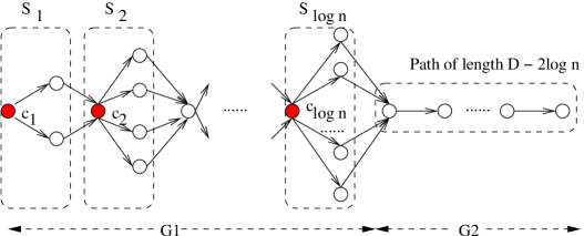
Figure 2: The network used in the lowerbound proof

We assume that $c_{1}$ is the originator of the broadcast. The purpose of $G_{1}$ is to show that every informed node in $G$ must be active for at least $\ln^{2}n$ rounds in order to complete broadcasting with probability $1-n^{-1}$. More specifically, no matter what $\alpha$ is, there is always a star $S_{i}$ such that the probability to inform $c_{i+1}$ is at most $1/\ln n$. Since our distribution is time invariant and every node does not know which star it belongs to, every node in the network needs to be active for at least $\ln^{2}n$ rounds. Let $\mu$ be the mean of distribution $\alpha$ and $ran(\alpha)$ be the set of outcomes of $\alpha$. Next, we use $G_{2}$ to argue that in order to finish broadcasting in $cD\log(n/D)$ rounds, $\mu$, mean of $\alpha$, must be at least $1/(2c\log(n/D))$. Hence, the total expected number of transmissions per node is at least $\ln^{2}n(1/(2c\log(n/D))>\log^{2}n/(4c\log(n/D))$.

Let $A_{i}$ be the event that $c_{i+1}$ is informed in Round $t_{i}$ under the condition that every leaf node of $S_{i}$ is active (note that they are always activated at the same time). Let $Q_{t_{i}}$ be the random variable that represents the probability chosen at Round $t_{i}$. Note that $Q_{t_{i}}$ has distribution $\alpha$. For any $q\in ran(\alpha)$, let $\Pr[A_{i}|Q_{t_{i}}=q]$ be the probability to inform $c_{i+1}$ if $Q_{t_{i}}=q$. Since $c_{i+1}$ is informed if exactly one of the $2^{i}$ leaf nodes of $S_{i}$ transmits we get

$$\Pr[A_{i}|Q_{t_{i}}=q]=2^{i}q(1-q)^{2^{i}-1}<2^{i}qe^{-(2^{i}-1)q}.$$ (4)

Observe that $\Pr[A_{i}]=\sum_{q\in ran(\alpha)}{(\Pr[Q_{t_{i}}=q]\Pr[A_{i}|Q_{t_{i}}=q])}$. We get,

$$\sum_{i=1}^{\log n}{\Pr[A_{i}]} = \sum_{i=1}^{\log n}\sum_{q\in ran(\alpha)}{\left(\Pr[Q_{t_{i}}=q]\Pr[A_{i}|Q_{t_{i}}=q]\right)}$$

$$= \sum_{q\in ran(\alpha)}{\left(\Pr[Q_{t_{i}}=q]\sum_{i=1}^{\log n}{\Pr[A_{i}|Q_{t_{i}}=q]}\right)}\leq\left(\sum_{q\in ran(\alpha)}{\Pr[Q_{t_{i}}=q]}\right)\frac{1}{\ln 2}=\frac{1}{\ln 2}.$$

For the third inequality, we use Equation 4 and $\forall 0\leq q\leq 1,\int_{1}^{\infty}2^{i}qe^{-(2^{i}-1)q}di=1/(e^{q}\ln 2)\leq 1/\ln 2$. Consequently,

$$\min_{i}{\Pr[A_{i}]}\leq\left(\sum_{i=1}^{\log n}{\Pr[A_{i}]}\right)/\log n\leq\frac{1}{\ln 2\log n}=\frac{1}{\ln n}.$$

Let $i^{*}=\arg\!\min_{i}{\Pr[A_{i}]}$. Consequently, in order to complete broadcasting with probability at least $1-n^{-1}$, every leaf node of $S_{i^{*}}$ must be active for at least $\ln^{2}n$ rounds.

In the following we show $\mu\geq 1/(2c\log(n/D))$ using $G_{2}$. First note that $L=D-2\log n>D/2$ since $D\geq 4\log n$. For any $0\leq i\leq L-1$, let $T_{i}$ be the number of rounds that $v_{i}$ is the highest ranked node on the path that is informed. Note that $T_{i}$ is geometrically distributed with probability $\mu$, we have $E[\sum_{i=0}^{L-1}{T_{i}}]=L\cdot E[T_{i}]=L/\mu$. Hence, in order to inform $v_{L}$ within $cD\log(n/D)$ steps (even expectedly), we need $\mu\geq 1/(2c\log(n/D))$ since $L>D/2$.

We have shown that every node in the network needs to be active for $\ln^{2}n$ rounds while in each round, the expected number of transmissions it performs is at least $1/(2c\log(n/D))$. Hence, the total expected number of transmissions per node is $(\ln^{2}n)(1/(2c\log(n/D)))>\log^{2}n/(4c\log(n/D))$. $\square$

Setting $D=n$ in the network constructed above, we immediately get the following corollary.

Corollary 4.5

There exists a network with $O(n)$ nodes such that any randomised oblivious broadcasting algorithm that finishes broadcasting in $cn$ rounds with probability at least $1-n^{-1}$ requires an expected number of $\Omega(\log^{2}n)$ transmissions.

Appendix

Appendix A Chernoff Bounds

Here we present a version of Chernoff bounds, which can be found, for example, in, [21].

Lemma A.1

Let $X_{1},\ldots X_{n}$ be independent Bernoulli random variables and let $X=\sum_{i=1}^{n}{X_{i}}$ and $\mu=E[X]$. Then we have,

1. $\Pr\left[X<(1-\epsilon)\mu\right]<e^{-\mu\epsilon^{2}/2}$, for $0\leq\epsilon\leq 1$.

2. $\Pr\left[X>(1+\epsilon)\mu\right]<e^{-\mu\epsilon^{2}/3}$, for $\epsilon>0$.

3. $\Pr\left[|X-\mu|\leq\epsilon\mu\right]>1-2e^{-\mu\epsilon^{2}/3}$, for $0\leq\epsilon\leq 1$.

Appendix B Proof of Lemma 2.3

Proof:  We consider two cases of different values of $p$. If $p>1/2$, we have $T=1$ and every node will have expectedly $(n-1)/2$ neighbours. The result now follows from a simple application of Chernoff bounds. If $p\leq 1/2$, we fix an arbitrary node $u$ and a round $t=1$ in Phase 1. First we bound $q$, the probability that $u$ is informed in Round $t$, i. e. $u$ is connected to exactly one node in $U_{t}$.

$$q=|U_{t}|p(1-p)^{|U_{t}|-1}>p|U_{t}|(1-p)^{1/p}\geq p|U_{t}|/4.$$ (5)

Here, the first inequality uses the condition $|U_{t}|<1/p$. To see the second one, note that $\forall 0<p<1/2,(1-p)^{1/p}>1/4$. Next, we show $N_{t}$, the number of not informed nodes at time $t$, is larger than $n/2$. By Observation 2.2$(2)$,

$$N_{t}=n-\left(\sum_{i=1}^{t-1}{|Q_{i}|}+|U_{t}|\right)>n-t|U_{t}|>n-(\log n)(1/p)>n/2.$$ (6)

Here, the first inequality is true by Observation 2.2$(1)$ and $|U_{1}|<|U_{2}|<\ldots<|U_{t}|$. The second one uses the condition $|U_{t}|<1/p$ and $t\leq T=\lfloor\log n/\log d\rfloor\leq\log n$. The third inequality uses $p>\delta\log n/n$. Hence,

$$E[|U_{t+1}|]=N_{t}q>(n/2)\cdot q\geq(n/2)\cdot p|U_{t}|/4=d|U_{t}|/8,$$

since $N_{t}>n/2$ and $d=np$. Note that the events to be connected to exactly one node in $U_{t}$ are independent for different not informed nodes. Also, note that each event is only evaluated once due to Observation 2.2(4). Using Chernoff bounds we get

$$\Pr[U_{t+1}|\leq d|U_{t}|/16]\leq\Pr[|U_{t+1}|\leq E[|U_{t+1}|]/2]\leq e^{-d|U_{t}|/64}=o(n^{-4}).$$

The last inequality uses $d=np$ with $p=\delta\log n/n$ for a sufficiently large constant $\delta$. Consequently $|U_{t+1}|/|U_{t}|>d/16$ with a probability $1-o(n^{-4})$. Using a similar approach, we can prove that $|U_{t+1}|/|U_{t}|<2d$ with a probability $1-o(n^{-4})$. This finished the proof of Part 1 of the lemma.

To prove part 2 we first need a tighter bound on $q$. By Equation 5,

$$q=|U_{t}|p\cdot(1-p)^{|U_{t}|-1}>(1-p|U_{t}|)\cdot p|U_{t}|>\left(1-1/\log n\right)\cdot p|U_{t}|$$

Next we bound $N_{t}$. Using Equation 6 with $|U_{t}|<1/(p\log n)$ and $t\leq T=\lfloor\log n/\log d\rfloor\leq\log n$ we get

$$N_{t}=n-\left(\sum_{i=1}^{t-1}{|Q_{i}|}+|U_{t}|\right)>n-t|U_{t}|>n-1/p>n\left(1-1/\log n\right).$$

Now, we obtain the following lower bound for $E[|U_{t+1}|]$,

$$E[|U_{t+1}|]=N_{t}q>\left(1-1/\log n\right)^{2}\cdot d|U_{t}|>\left(1-2/\log n\right)\cdot d|U_{t}|.$$

For an upper bound on $E[|U_{t+1}|]$ we use $N_{t}<n$ and $q\leq p|U_{t}|$ to get

$$E[|U_{t+1}|]=N_{t}q<np|U_{t}|=d|U_{t}|.$$

Using Chernoff bounds together with the assumption that $|U_{t}|>\log^{3}n$, we get

$$\Pr\left[\left(1-3/\log n\right)d|U_{t}|<|U_{t+1}|<\left(1+1/\log n\right)d|U_{t}|\right]>1-2e^{-\frac{E[|U_{t+1}|]}{4\log^{2}n}}=1-o\left(n^{-4}\right).$$

$\square$

Appendix C Proof of Lemma 3.2

The proof is similar to the proof of Lemma $3.4$ in [10]. All that we have to do is to bound the probability $q$ that a node successfully sends a message to a fixed neighbour. The expected degree of every node is $d$ and using Chernoff bounds we can show the degree of every node is at most $2d$ with a probability $1-o(n^{-5})$. Hence, with a probability $1-o(n^{-5})$, we have

$$q_{r}\geq(1/d)(1-1/d)^{2d-1}\geq(1/d)\cdot(1-1/d)^{2d}\geq(1/d)\cdot(1/4)^{2}=1/(16d).$$

$\square$

Now it remains to bound $\Pr[\sum_{i=1}^{L}{Y_{i}}\leq 128d\log n]$. Similar to the proof of Lemma $3.5$ of [10], applying the standard relation of geometric distribution and binomial distributions, and using Chernoff bounds on the corresponding binomial distribution, we get

$$\Pr\left[\sum_{i=1}^{L}{Y_{i}}>128d\log n\right]\leq\Pr\left[{\mathbb{B}}(128d\log n,1/(16d))<L\right]\leq e^{-(7/8)^{2}\cdot 8\log n/2}<e^{-3\log n}=o(n^{-3}).$$

The third inequality holds since $L\leq D<\log n$. The bound on the gossiping time follows by the union bound and the fact that there are in total $n(n-1)$ source-destination pairs.

Next we bound the number of transmissions. Let $v$ be an arbitrary node and denote $Z_{v}$ to be the number of transmissions performed by $v$. Note that $E[Z_{v}]=128\log n$ since in each round, every node transmits with probability $1/d$ and our algorithm has in total $128d\log n$ rounds. Using Chernoff bounds we get that $Z_{v}\leq 256\log n$ with probability $1-o(n^{-2})$. By the union bound, we get with a probability $1-o(n^{-1})$, none of the nodes performs more than $256\log n$ transmissions.

Appendix D Proof of Observation 4.3

We construct a network with $3n+1$ nodes. $s$ is the node initiating the broadcast, and $d_{1},\ldots,d_{n}$ are the destination nodes. $s$ has an edge to $2n$ intermediate nodes $u_{1},\ldots u_{2n}$. For all $1\leq i\leq n$, $d_{i}$ connects to both $u_{2i-1}$ and $u_{2i}$. Let us assume that $s$ informs $u_{1},\ldots,u_{2n}$ in Round $t_{1}$. Now fix some arbitrary $T>t_{1}$. In Round $t_{1}+1\leq r\leq T$, let $q_{r}$ be the send probability used by the algorithm. For all $1\leq i\leq n$, the probability to inform node $d_{i}$ in Round $r$ is $2q_{r}(1-q_{r})$. Due to symmetry we can assume that $q_{r}\leq 1/2$, resulting in $(1-q_{r})^{1/q_{i}}\geq 1/4$. Hence,

$$\Pr[d_{i}\mbox{ is not informed before Round $T$}] = \prod_{r=t_{1}+1}^{T}{\left(1-2q_{r}(1-q_{r})\right)}$$

$$>\prod_{r=t_{1}+1}^{T}{(1-q_{r})^{2}} \geq \prod_{r=t_{1}+1}^{T}{4^{-2q_{r}}}=2^{-4\sum_{r=t_{1}+1}^{T}{q_{r}}}.$$

Now it is easy to see that, to inform $d_{i}$ with probability $1-n^{-1}$, we need $\sum_{r=t_{1}+1}^{T}{q_{r}}>\log n/4$. Note that $\sum_{r=t_{1}+1}^{T}{q_{r}}$ is the expected number of transmissions that $u_{i}$ and $v_{i}$ perform between Round $t_{1}+1$ and $T$. The total number of transmissions performed by all $2n$ intermediate nodes is at least $2n\ (\log n/4)=n\log n/2$.

References

- [1] William Aiello, Fan Chung and Linyuan Lu. A random graph model for massive graphs, Proc. 32nd ACM Symposium on Theory of Computing (STOC), Portland, Oregon, USA, pp. 171–180, 2000.
- [2] Noga Alon, Amotz Bar-Noy, Nathan Linial and David Peleg. A Lower Bound for Radio Broadcast. Journal of Computer and System Sciences, vol. 43, num. 2, pp. 290–298, 1991.
- [3] Reuven Bar-Yehuda, Oded Goldreich and Alon Itai. On the Time-Complexity of Broadcast in Multi-hop Radio Networks, An Exponential Gap Between Determinism and Randomization. Journal of Computer and System Sciences vol. 45, num. 1, pp. 104-126, 1992.
- [4] Belá Bollobás. The diameter of random graphs. IEEE Transaction on Information Theory, vol. 36, num. 2, pp. 285–288, 1990.
- [5] Bogdan S. Chlebus, Dariusz R. Kowalski and Mariusz A. Rokicki. Average-Time Complexity of Gossiping in Radio Networks. Proc 13th Colloquium on Structural Information and Communication Complexity (SIROCCO), pp. 253-267, 2006.
- [6] Marek Chrobak, Leszek Gasieniec and Wojciech Rytter. Fast Broadcasting and Gossiping in Radio Networks. Proc. 41st Annual IEEE Symposium on Foundations of Computer Science (FOCS), Redondo Beach, CA, USA, pp. 575–581, 2000.
- [7] Marek Chrobak and Leszek Gasieniec and Wojciech Rytter., A Randomized Algorithm for Gossiping in Radio Networks. Proc 7th Annual International Computing and Combinatorics Conference (COCOON), pp. 483–492. 2001.
- [8] Fan Chung and Linyuan Lu. The diameter of random sparse graphs. Adv. in Appl. Math, vol. 26, num. 4, pp. 257–279, 2001.
- [9] Andrea E. F. Clementi, Angelo Monti and Riccardo Silvestri. Selective families, superimposed codes, and broadcasting on unknown radio networks. Proc. 12th ACM Symposium on Discrete Algorithms (SODA), Washington, D.C., USA, pp. 709–718, 2001.
- [10] Artur Czumaj and Wojciech Rytter. Broadcasting Algorithms in Radio Networks with Unknown Topology. Journal of Algorithms, vol. 60, num. 2, pp. 115–143, 2006.
- [11] Robert Elsässer and Leszek Gasieniec. Radio Communication on random graphs. Proc. 17th ACM Symposium on Parallelism in Algorithms and Architectures (SPAA), Las Vagas, NV, USA, pp. 309–315, 2005
- [12] R. Elsässer. On the Communication Complexity of Randomized Broadcasting in Random-like Graphs. Proc. 18th ACM Symposium on Parallelism in Algorithms and Architectures (SPAA), Cambridge, Massachussetts, USA, pp. 148–157, 2006.
- [13] Wendi Rabiner Heinzelman, Joanna Kulik and Hari Balakrishnan. Adaptive Protocols for Information Dissemination in Wireless Sensor Networks. Proc. 5th Annual ACM/IEEE International Conference on Mobile Computing and Networking (MOBICOM), Seattle, WA, USA, pp. 174–185., 1999.
- [14] Lefteris M. Kirousis, Evangelos Kranakis, Danny Krizanc and Andrzej Pelc. Power Consumption in Packet Radio Networks (Extended Abstract). Proc. 14th Symposium on Theoretical Aspects of Computer Science (STACS), Hansestadt Lübeck, Germany, pp. 363-374, 1997.
- [15] Dariusz R. Kowalski and Andrzej Pelc. Deterministic Broadcasting Time in Radio Networks of Unknown Topology.. Proc. 43rd Annual IEEE Symposium on Foundations of Computer Science (FOCS), Vancouver, BC, Canada, pp. 63–72, 2002.
- [16] Dariusz R. Kowalski and Andrzej Pelc. Broadcasting in undirected ad hoc radio networks. Proc 24th Symposium on Principles of Distributed Computing (PODC) Boston, Massachusetts, USA, pp. 73–82, 2003.
- [17] Eyal Kushilevitz and Yishay Mansour. An Lower Bound for Broadcast in Radio Networks., SIAM Journal on Computing, vol. 27, num. 3, pp. 702–712, 1998.
- [18] Ding Liu and Manoj Prabhakaran. On Randomized Broadcasting and Gossiping in Radio Networks. Proc 8th Annual International Computing and Combinatorics Conference (COCOON), Singapore, pp. 340–349, 2002.
- [19] Linyuan Lu. The diameter of random massive graphs. Proc. 12th ACM Symposium on Discrete Algorithms (SODA), Washington, D.C., USA, pp. 912–921, 2001.
- [20] Samuel Madden, Michael J. Franklin, Joseph M. Hellerstein and Wei Hong. TAG: A Tiny Aggregation Service for Ad-Hoc Sensor Networks. Proc. 5th Symposium on Operating Systems Design and Implementation (OSDI), Boston, MA, USA, pp. 131 - 146, 2002.
- [21] Michael Mitzenmacher and Eli Upfal. Probability and Computing Cambridge Press, 2005.
- [22] Ying Xu. An deterministic gossiping algorithm for radio networks. algorithmica, vol. 36, num. 1, pp. 93–96,2003.