Synchronization recovery and state model reduction for soft decoding of variable length codes

Abstract

Variable length codes (VLCs) exhibit de-synchronization problems when transmitted over noisy channels. Trellis decoding techniques based on Maximum A Posteriori (MAP) estimators are often used to minimize the error rate on the estimated sequence. If the number of symbols and/or bits transmitted are known by the decoder, termination constraints can be incorporated in the decoding process. All the paths in the trellis which do not lead to a valid sequence length are suppressed. This paper presents an analytic method to assess the expected error resilience of a VLC when trellis decoding with a sequence length constraint is used. The approach is based on the computation, for a given code, of the amount of information brought by the constraint. It is then shown that this quantity as well as the probability that the VLC decoder does not re-synchronize in a strict sense, are not significantly altered by appropriate trellis states aggregation. This proves that the performance obtained by running a length-constrained Viterbi decoder on aggregated state models approaches the one obtained with the bit/symbol trellis, with a significantly reduced complexity. It is then shown that the complexity can be further decreased by projecting the state model on two state models of reduced size.

I Introduction

VLCs are widely used in compression systems due to their high compression efficiency. One drawback of VLCs is their high sensitivity to errors. A single bit error may lead to the de-synchronization of the decoder. Nevertheless, many VLCs exhibit self-synchronization properties. The authors in [1] show such properties for some binary Huffman codes. The error recovery properties of VLCs have also been studied in [2], where a method to compute the so-called expected error span $E_{s}$ (i.e. the expected number of source symbols on which a single bit error propagates), has been proposed. The same quantity has been called mean error propagation length (MEPL) in [3]. The authors in [4] consider the variance of the error propagation length (VEPL) to assess the resilience of a code with hard decoding techniques. In [5], the method of [2] is extended to compute the so-called synchronization gain/loss, i.e. the probability that the number of symbols in the transmitted and decoded sequences differ by a given amount $\Delta S$ when a single bit error occurs during the transmission. Note that various VLC constructions have also been proposed to improve the self-synchronization properties of the codes [6], [7], [8]. The author in [7] introduces a method to construct prefix-free self-synchronizing VLCs called T-codes. The synchronization property of these codes is analyzed in [9] in terms of the expected synchronization delay.

VLC soft decoding techniques based on MAP (or MMSE) estimators have also been considered to minimize the error rates (or distortion) observed on the decoded sequences. The approaches essentially differ in the optimization metrics as well as in the assumptions made on the source model and on the information available at the decoder. These assumptions lead to different trellis structures on which the estimation or soft-decoding algorithms are run. Two main types of trellises are considered to estimate the sequence of emitted symbols from the received noisy bitstream: the bit-level trellis proposed in [10] and the bit/symbol trellis. The bit-level trellis leads to low decoding complexity. However, it does not allow the exploitation of extra information, such as the number of emitted symbols. It hence suffers from some suboptimality. If the knowledge of the number of emitted symbols is available at the decoder, the problem is referred to as soft decoding with length constraint and is addressed, e.g., in [11][12][13][14]. This problem has led to the introduction of the bit/symbol trellis in [15]. This trellis can optimally exploit such constraints, leading to optimal performance in terms of error resilience. Nevertheless, the number of states of the bit/symbol trellis is a quadratic function of the sequence length. The corresponding complexity is actually not tractable for typical sequence lengths. In order to overcome this complexity hurdle, most authors apply suboptimal estimation methods on this optimal state model such as sequential decoding [14][16][17].

This paper presents a method to assess the error resilience of VLCs when trellis decoding with length constraint is used at the decoder side. The approach is based on the concept of gain polynomials defined on error state diagrams introduced in [2] and [5]. The method introduced in [5] to compute the synchronization gain/loss is first recalled. This method is then extended to the case of a symbol sequence of length $L(S)$ being sent over a binary symmetrical channel (BSC) of a given crossover probability. The derivation is inspired from the matricial method described in [3]. It has been shown in [18][19] that the Markovian property of a source can be easily integrated in the source model by expanding the state model by a constant factor. We thus restrict the analysis to memoryless sources. It is shown that for VLCs, the probability mass function (p.m.f.) of the synchronization gain/loss is a key indicator of the error resilience of such codes when soft decoding with length constraint is applied at the decoder side. The p.m.f. of the gain/loss allows the computation of the probability that the symbol length of the decoded sequence is equal to $L(S)$, i.e. the probability that the decoder resynchronizes in the strict-sense (no gain nor loss of symbols during the transmission). This quantity is given by ${\mathbb{P}}(\Delta S=0)$. The length constraint is used to discard all decoded sequences which do not satisfy the constraint $\Delta S=0$. If $P(\Delta S=0)$ is high, the number of “de-synchronized” sequences which will be discarded will be high. This results in increasing the likelihood of the correct sequence, hence in decreasing the decoding error rate. The entropy of the p.m.f. of the gain/loss represents the amount of information that the length constraint brings to the decoder. These two quantities (${\mathbb{P}}(\Delta S=0)$ and $H(\Delta S)$) are shown to better predict the relative decoding performance of VLCs when soft decoding with a length constraint is used,than the MEPL and VEPL measures (these measures are appropriate when hard decoding is used). Note that, in the following, the term MEPL will be used to refer to the expectation of the error propagation length.

This analysis is then used in Section III to assess the performance of MAP decoding on the aggregated state models proposed in [20], for jointly typical source/channel realizations. The aggregated state model is defined by both the internal state of the VLC decoder (i.e., the internal node of the VLC codetree) and the remainder of the Euclidean division of the symbol clock values by a fixed parameter called $T$. This model aggregates states of the bit/symbol trellis which differs by multiple of $T$symbol clock instants. The parameter $T$ controls the trade-off between estimation accuracy and decoding complexity. The choice of this parameter has indeed an impact on the quantity of information brought by the length constraint on the corresponding trellis. It is shown that the probability that the VLC decoder does not re-synchronize in a strict sense, as well as the entropy of the constraint, are not significantly altered by aggregating states, provided that the aggregation parameter $T$ is greater than or equal to a threshold. An upper bound of this threshold is derived according to the analysis of Section II. This proves that the performance obtained by running a length-constrained Viterbi decoder on the aggregated trellis closely approaches the performance obtained on the bit/symbol trellis, with a significantly reduced complexity. Finally, it is shown in Section IV that the decoding complexity can be further reduced by considering separate estimations on trellises of smaller dimensions, whose parameters $T_{1}$ and $T_{2}$ are relatively prime. If the two sequence estimates are not equal, the decoding on a trellis of parameter $T_{1}\times T_{2}$ is then computed. The equivalence in terms of decoding performance between this approach, referred to as combined trellis decoding, and the decoding on a trellis of parameter $T_{1}\times T_{2}$ is proved for the MAP criterion, i.e. for the Viterbi algorithm [21].

II Link between VLC synchronization recovery properties and soft decoding performance with a length constraint

Let ${\mathbf{S}}=S_{1},...S_{t},...S_{L({\mathbf{S}})}$ be a sequence of $L({\mathbf{S}})$ symbols. This sequence is encoded with a VLC ${\mathcal{C}}$, producing a bitstream ${\mathbf{X}}=X_{1},...X_{k},...X_{L({\mathbf{X}})}$ of length $L({\mathbf{X}})$. This bitstream is modulated using a binary phase shift keying (BPSK) modulation and is transmitted over an additive white Gaussian noise (AWGN) channel, without any channel protection. The channel is characterized by its signal to noise ratio, denoted ${E_{b}}/{N_{0}}$ and expressed in decibels (dB). Note that we reserve block capital letters to represent random variables and small letters to represent their corresponding realizations. In this paper, the term polynomial refers to expressions of the form $\sum_{i\in{\mathbb{Z}}}a_{i}x^{i}$, where $x$ denotes the variable and $a_{i}$ are polynomial coefficients. Hence, we include in this terminology either polynomial series (with an infinite number of non null coefficients) or finite length polynomials (such as $\exists N\in{\mathbb{N}}\,\,|\,\,\forall n>N,\ a_{-i}=a_{i}=0$), both with negative powers.

II-A The gain/loss behavior of a variable length code

A method to compute the so-called expected error span $E_{s}$ following a single bit error has been introduced in [2]. This method relies on an error state diagram which represents the states of the decoder when the encoder is in the root node. Hence, the error state diagram includes the internal states of the decoder, i.e. the internal nodes of the VLC, plus two states which represent the loss of synchronization state $n_{l}$ and the return to synchronization state $n_{s}$ respectively. Therefore, the set of states of the diagram is $\{n_{l},n_{\alpha_{1}},n_{\alpha_{2}},...,n_{s}\}$, where the set $\{\alpha_{1},\alpha_{2},...\}$ represents the set of prefixes of the VLC. The state $n_{s}$ of the error state diagram corresponds to a return of both encoder and decoder automata to the root node of the code tree. However, this state may not correspond to a strict sense synchronization. In other words, the number of decoded symbols may be different from the number of emitted ones. The branches of the error state diagram represent the transitions between two states of the decoder when a single source symbol has been emitted by the encoder. They are labeled by an indeterminate variable $z$ which corresponds to the encoding of one source symbol. Hence, the gain along each edge is the probability of the transition associated with that edge multiplied by $z$. In that case, the gain on the diagram from $n_{l}$ to $n_{s}$ (i.e. the transfer function between $n_{l}$ and $n_{s}$) is a polynomial of the variable $z$ such that the coefficient of $z^{i}$ is the probability that the considered VLC resynchronizes after exactly $i$ source symbols following the bit error. Evaluating the derivative of the gain polynomial at $1$ provides the expected error span $E_{s}$.

The branch labeling of the error state diagram has been extended in [5] so that the gain polynomial informs about the difference, caused by a single bit error, between the number of emitted and decoded symbols, after hard decoding of the received bitstream. This quantity, denoted $\Delta S$, is referred to as the gain/loss. In order to evaluate the p.m.f. of the random variable $\Delta S$, a new variable $y^{j}$ is introduced in the branch labeling of the error state diagram. The exponent $j$ represents the number of extra output symbols for each input symbol. Hence, the corresponding gain polynomial $G(y,z)$ is function of both variables $y$ and $z$. Evaluating this polynomial at $z=1$ gives a polynomial in $y$ only. For sake of clarity, we simply denote this polynomial as

$$G(y)=G(y,z)|_{z=1}.$$ (1)

The coefficient of $y^{i}$ in the polynomial $G(y)$ gives the probability ${\mathbb{P}}(\Delta S=i)$ following one bit error. Note that $i$ can be negative if the decoded sequence is longer than the encoded one. In this section, we focus on the behavior of the polynomial $G(y)$. Since the variable $z$ is not necessary, we compute directly the state diagram for $z=1$.

Let $\overline{H}$ be the transition matrix corresponding to the error state diagram.

$$\overline{H}=\left(\begin{array}[]{cccc}{\mathbb{P}}(n_{l}|n_{l})&{\mathbb{P}}(n_{\alpha_{1}}|n_{l})&\cdots&{\mathbb{P}}(n_{s}|n_{l})\\ {\mathbb{P}}(n_{l}|n_{\alpha_{1}})&{\mathbb{P}}(n_{\alpha_{1}}|n_{\alpha_{1}})&\cdots&{\mathbb{P}}(n_{s}|n_{\alpha_{1}})\\ \vdots&\vdots&\ddots&\vdots\\ {\mathbb{P}}(n_{l}|n_{s})&{\mathbb{P}}(n_{\alpha_{1}}|n_{s})&\cdots&{\mathbb{P}}(n_{s}|n_{s})\\ \end{array}\right)$$ (2)

where ${\mathbb{P}}(n_{\alpha_{i}}|n_{\alpha_{j}})$ represents the probability to go to state $n_{\alpha_{i}}$ from state $n_{\alpha_{j}}$. Let us call $h_{i,j}^{k}(y)$ the element at row $i$ and column $j$ of the matrix $\overline{H}^{k}$. Note that $h_{i,j}^{k}(1)$ is the probability to go from state $n_{\alpha_{i}}$ to state $n_{\alpha_{j}}$ in $k$ stages, i.e. after the encoding of $k$ source symbols. The top right elements of the matrices $\overline{H}$ and $\overline{H}^{k}$ are respectively denoted $h(y)={\mathbb{P}}(n_{s}|n_{l})$ and $h^{k}(y)$. The gain polynomial $G(y)$ can then be written as

$$G(y)=\sum_{k\in\mathbb{N}^{*}}h^{k}(y).$$ (3)

Hence, the gain polynomial $G(y)$ is obtained as the top right element of the matrix $(\overline{I}-\overline{H})^{-1}$, where $\overline{I}$ denotes the identity matrix of the same dimensions as $\overline{H}$. Note that this property holds if $(\overline{I}-\overline{H})^{-1}$ exists.

Let us consider the $5$-symbol source and the 16 VLCs used in [3] to illustrate these concepts. The probability of this source as well as the different codes are reproduced in Table I. These codes have the same mean description length of $2.2$ bits per symbols.

TABLE I: Source and Codes from [3] used in this paper.

$$\begin{array}[]{|c|ccccc|}\hline\cr a_{i}&a_{1}&a_{2}&a_{3}&a_{4}&a_{5}\\ \hline\cr{\mathbb{P}}(a_{i})=&0.4&0.2&0.2&0.1&0.1\\ \hline\cr{\mathcal{C}}_{1}&00&01&10&110&111\\ {\mathcal{C}}_{2}&00&01&11&100&101\\ {\mathcal{C}}_{3}&00&10&11&010&011\\ {\mathcal{C}}_{4}&01&00&10&110&111\\ {\mathcal{C}}_{5}&01&00&11&100&101\\ {\mathcal{C}}_{6}&01&10&11&000&001\\ {\mathcal{C}}_{7}&0&10&110&1110&1111\\ {\mathcal{C}}_{8}&0&10&111&1100&1101\\ {\mathcal{C}}_{9}&0&11&100&1010&1011\\ {\mathcal{C}}_{10}&0&11&101&1000&1001\\ {\mathcal{C}}_{11}&0&100&101&110&111\\ {\mathcal{C}}_{12}&0&100&110&101&111\\ {\mathcal{C}}_{13}&0&100&111&110&101\\ {\mathcal{C}}_{14}&0&101&110&100&111\\ {\mathcal{C}}_{15}&0&101&111&100&110\\ {\mathcal{C}}_{16}&0&110&111&100&101\\ \hline\cr\end{array}$$

Example 1: Let us consider the code ${\mathcal{C}}_{5}$. Its state diagram is depicted in Fig. 1. The transition matrix derived from the previous guidelines, i.e. by setting the variable z to 1 in the extended diagram of [5], is given by

$$\overline{H}_{{\mathcal{C}}_{5}}=\left(\begin{array}[]{ccccc}0&\frac{1}{11}&\frac{1}{11}&\frac{2y}{11}&\frac{7}{11}\\ 0&\frac{1}{5}&\frac{3}{5}&0&\frac{y^{-1}}{5}\\ 0&0&\frac{1}{5}&0&\frac{3+y^{-1}}{5}\\ 0&\frac{1}{5}&\frac{3}{5}&0&\frac{y^{-1}}{5}\\ 0&0&0&0&0\\ \end{array}\right).$$

This leads to $G(y)=0.0625y^{-1}+0.8352+0.1023y$, which also means that

$$\left\{\begin{array}[]{ll}{\mathbb{P}}(\Delta S=-1)&=0.1023\\ {\mathbb{P}}(\Delta S=0)&=0.8352\\ {\mathbb{P}}(\Delta S=1)&=0.0625.\end{array}\right.$$ (4)

Figure 1: Error state diagram of [5] for the code ${\mathcal{C}}_{5}$. The transition probabilities are denoted next to the branches.

II-B Extension to the BSC

Let us recall that $\Delta S$ corresponds to the gain/loss engendered by a single bit error. We propose here to estimate ${\mathbb{P}}(\Delta S=i)$ for a sequence of $L({\mathbf{S}})$ symbols that has been sent through a BSC of crossover probability $p$ (equals to the bit error rate). Since in this section the VLC decoder is assumed to be a classical hard decoder, the analysis is also valid on an AWGN channel characterized by its signal to noise ratio $E_{b}/N_{0}$ by taking $\textrm{p}=\frac{1}{2}\textrm{erfc}\left(\sqrt{\frac{E_{b}}{N_{0}}}\right)$.

For a sequence of $L({\mathbf{S}})$ symbols, the bitstream length $L({\mathbf{X}})$ lies in the interval of integers ${\mathcal{I}}=\{L({\mathbf{S}})\times l_{m},\dots,L({\mathbf{S}})\times\,l_{M}\}$, where $l_{m}$ and $l_{M}$ respectively denote the lengths of the shortest and longest codewords. Let $E$ denote the random variable corresponding to the number of errors after the hard decoding of the received bitstream ${\mathbf{Y}}$. For $i\in{\mathbb{Z}}$, the probability ${\mathbb{P}}(\Delta S=i)$ is given by

$${\mathbb{P}}(\Delta S=i)=\sum_{e\in{\mathbb{N}}}{\mathbb{P}}(\Delta S=i\,|\,E=e){\mathbb{P}}(E=e).$$ (5)

For $e\in{\mathbb{N}}$, the probability ${\mathbb{P}}(E=e)$ can be expressed as

$${\mathbb{P}}(E=e)=\sum_{k\in{\mathcal{I}}}{\mathbb{P}}(E=e| L({\mathbf{X}})=k){\mathbb{P}}(L({\mathbf{X}})=k)$$ (6)

$$\textrm{if }e\leq L(S)\times l_{M}$$ (7)

$$\textrm{otherwise }{\mathbb{P}}(E=e)=0,$$ (8)

where the quantities ${\mathbb{P}}(E=e|L({\mathbf{X}})=k)$ only depend on the signal to noise ratio and are equal to

$$\left\{\begin{array}[]{lll}{\mathbb{P}}(E=e|L({\mathbf{X}})=k)&={k\choose e}\,\textrm{p}^{e}\,(1-\textrm{p})^{i-e}&\textrm{if }e\leq k\\ {\mathbb{P}}(E=e|L({\mathbf{X}})=k)&=0&\textrm{if }e>k.\end{array}\right.$$ (9)

For every $k\in{\mathcal{I}}$, the probability ${\mathbb{P}}(L({\mathbf{X}})=k)$ is calculated from the source statistics and the code ${\mathcal{C}}$ structure.

To calculate ${\mathbb{P}}(\Delta S=i)$ according to Eqn. 5, we now need to compute the quantities ${\mathbb{P}}(\Delta S=i\,|\,E=e)$. For that purpose, let us now assume that the decoder has already recovered from previous errors when another error occurs. This assumption requires that the probability that an error occurs when the decoder has not returned to the synchronization state $n_{s}$ is very low. The lower the error span is and the higher $E_{b}/N_{0}$ is, the more accurate this approximation is. Under this assumption, the quantity $\Delta S$ is independently impacted by multiple errors.

Let us define

$$G_{e}(y)=(\underbrace{G\star...\star G}_{e\text{ times}})(y)=\sum_{i\in\mathbb{Z}}a_{i,e}y^{i},$$ (10)

where $\star$ denotes the convolution product. Note that the polynomial $G_{1}=G$ corresponds to the gain polynomial of Eqn. 3. Under the previous assumption, the quantity $a_{i,e}$ equals ${\mathbb{P}}(\Delta S=i|E=e)$. With Eqn. 8, the resulting gain polynomial for this crossover probability can be expressed as

$${\tilde{G}}(y) =\sum_{e\in\mathbb{N}}G_{e}(y)\,{\mathbb{P}}(E=e),$$ (11)

where only the quantity ${\mathbb{P}}(E=e)$ depends on $E_{b}/N_{0}$. The coefficients ${\tilde{g}_{i}}$ of $\tilde{G}$ verify

$${\tilde{g}_{i}} =\sum_{e\in\mathbb{N}}a_{i,e}\,{\mathbb{P}}(E=e)$$ (12)

$$=\sum_{e\in\mathbb{N}}{\mathbb{P}}(\Delta S=i|E=e){\mathbb{P}}(E=e)$$ (13)

$$={\mathbb{P}}(\Delta S=i).$$ (14)

Let $\eta>0$ be a criterion of negligibility. For a given $\eta$, the pseudo-degree $d_{\eta}$ of the polynomial $\tilde{G}$ is defined as

$$d_{\eta}=^{\Delta}\min_{\mathbb{N^{*}}}\,d\,\,{\Big{|}}{\sum_{i\in{\mathbb{Z}}-\{-d,...,d\}}\tilde{g}_{i}<\eta}.$$ (15)

The pseudo-degree $d_{\eta}$ of a polynomial is the degree beyond which the sum of the coefficients of this polynomial are below a given threshold $\eta$.

Example 2: Let us determine the pseudo-degree such that $\eta=10^{-6}$ for the code ${\mathcal{C}}_{5}$, $E_{b}/N_{0}=\text{6\,dB}$, and $L({\mathbf{S}})=100$. The estimates of $\tilde{g}_{i}$ obtained from Eqn. 14 lead to

$${\small\left\{\begin{array}[]{ll}{\mathbb{P}}(\Delta S\leq-4)&=0.0000002\\ {\mathbb{P}}(\Delta S=-3)&=0.0000235\\ {\mathbb{P}}(\Delta S=-2)&=0.0013201\\ {\mathbb{P}}(\Delta S=-1)&=0.0493389\\ {\mathbb{P}}(\Delta S=0)&=0.9186664\\ {\mathbb{P}}(\Delta S=1)&=0.0301524\\ {\mathbb{P}}(\Delta S=2)&=0.0004930\\ {\mathbb{P}}(\Delta S=3)&=0.0000053\\ {\mathbb{P}}(\Delta S\geq 4)&=0.0000001.\end{array}\right.}$$ (16)

Hence, according to the definition of the pseudo-degree in Eqn. 15, $d_{\eta}=3$. The values of ${\mathbb{P}}(\Delta S=i)$ obtained by simulation and averaged over $10^{7}$ channel realizations are

$${\small\left\{\begin{array}[]{ll}{\mathbb{P}}(\Delta S\leq-4)&=0.0000002\\ {\mathbb{P}}(\Delta S=-3)&=0.0000207\\ {\mathbb{P}}(\Delta S=-2)&=0.0012587\\ {\mathbb{P}}(\Delta S=-1)&=0.0500770\\ {\mathbb{P}}(\Delta S=0)&=0.9185508\\ {\mathbb{P}}(\Delta S=1)&=0.0296306\\ {\mathbb{P}}(\Delta S=2)&=0.0004578\\ {\mathbb{P}}(\Delta S=3)&=0.0000041\\ {\mathbb{P}}(\Delta S\geq 4)&=0.0000001\end{array}\right.}$$ (17)

and also lead to $d_{\eta}=3$.
The simulated values of ${\mathbb{P}}(\Delta S=i)$ are close to the estimated ones for a large set of $E_{b}/N_{0}$ values, which validates the approximation. The pseudo-degrees for $\eta=10^{-6}$ of the codes introduced in Table I have been computed and are given in Table II.

TABLE II: Pseudo-degrees $d_{\eta}$ for $\eta=10^{-6}$, proposed criteria, criteria of [3], and error resilience performance for $E_{b}/N_{0}=\textrm{6\,db}$, and $L(S)=100$.

$$\begin{array}[]{|c|c|cc|cr|ccc|}\hline\cr\textrm{Code}&d_{\eta}&{\mathbb{P}}(\Delta S=0)&H(\Delta S)&\textrm{MEPL}\cite[cite]{[\@@bibref{}{ZhZ02}{}{}]}&\textrm{VEPL}\cite[cite]{[\@@bibref{}{ZhZ02}{}{}]}&\textrm{NLD}&\textrm{BER}&\textrm{FER}\\ \hline\cr{\mathcal{C}}_{1}&3&0.9185&0.499&3.89256&34.721&0.00877&0.00193&0.34053\\ {\mathcal{C}}_{2}&4&0.9005&0.578&2.02273&2.003&0.00632&0.00191&0.33641\\ {\mathcal{C}}_{3}&4&0.8971&0.595&2.06061&2.107&0.00626&0.00192&0.33636\\ {\mathcal{C}}_{4}&4&0.8913&0.608&4.07692&27.800&0.00759&0.00177&0.31548\\ {\mathcal{C}}_{5}&3&0.9187&0.497&1.71023&1.200&0.00586&0.00194&0.34296\\ {\mathcal{C}}_{6}&4&0.8996&0.578&3.54546&18.854&0.00758&0.00182&0.32368\\ {\mathcal{C}}_{7}&5&0.7088&1.287&1.55556&0.370&0.00619&0.00154&0.21849\\ {\mathcal{C}}_{8}&10&0.7006&1.553&2.34861&2.045&0.00646&0.00134&0.19543\\ {\mathcal{C}}_{9}&9&0.6703&1.632&1.95707&1.025&0.00571&0.00123&0.16739\\ {\mathcal{C}}_{10}&36&0.6401&2.267&6.18182&36.231&0.00483&0.00074&0.10354\\ {\mathcal{C}}_{11}&8&0.8797&0.655&1.85227&2.233&0.00614&0.00183&0.32219\\ {\mathcal{C}}_{12}&8&0.8882&0.620&1.71678&1.506&0.00617&0.00187&0.32951\\ {\mathcal{C}}_{13}&8&0.8860&0.634&1.79798&1.914&0.00615&0.00182&0.32142\\ {\mathcal{C}}_{14}&8&0.8957&0.599&2.03104&2.952&0.00666&0.00186&0.32698\\ {\mathcal{C}}_{15}&8&0.8941&0.610&2.20321&4.144&0.00685&0.00189&0.33244\\ {\mathcal{C}}_{16}&6&0.9044&0.564&1.98086&2.615&0.00672&0.00193&0.33829\\ \hline\cr\end{array}$$

II-C Code selection criteria

Let us consider a MAP estimation run on the bit/symbol trellis, with an additional constraint on the length of the decoded sequence. This length constraint is used to discard all decoded sequences having a number of symbols which differs from the number of transmitted symbols, that is, which does not satisfy the constraint $\Delta S=0$. On the bit/symbol trellis, the decoder has two kinds of information to help the estimation: the excess rate of the code and the information brougth by the length constraint. The excess rate of a VLC (residual redundancy in the encoded bitstream) is given by the difference between the mean description length (mdl) of the code and the entropy of the source. The information brougth by the length constraint on the bit/symbol trellis is given by the entropy of the p.m.f. of the gain/loss measure ($\Delta S$). For the considered set of codes, the excess rate is equal to $0.0781$ bits of information and is the same for all codes of Table I.

From the p.m.f. of $\Delta S$ the following two quantities can be computed:

• the probability ${\mathbb{P}}(\Delta S=0)$ to have a strict sense resynchronization

• the entropy $H(\Delta S)$.

If the probability ${\mathbb{P}}(\Delta S=0)$ is small, the number of “de-synchronized” sequences which will be discarded will be high, then the probability of detecting and correcting errors increases. This results in increasing the likelihood of the correct sequence, hence in decreasing the decoding error rate. As explained below, the entropy $H(\Delta S)$ measures the amount of information brought by the length constraint on the bit/symbol trellis. To design performance criteria for VLCs, we consider codes having the same mdl so that their performance can be fairly compared. Hence, the values ${\mathbb{P}}(\Delta S=0)$ and $H(\Delta S)$, computed from the p.m.f. of the gain/loss measure, are indicators of the performance of a VLC when soft decoding with length constraint is applied at the decoder side. Table II shows the values of these two quantities for the codes of Table I, together with the MEPL and the VEPL of [3]. The corresponding decoding performance in terms of the normalized Levenshtein distance (NLD) [22], BER and frame error rate (FER) obtained with the bit/symbol trellis, for $E_{b}$/$N_{0}$= 6dB and $L(S)=100$, are also given. It can be observed that the code $C_{10}$ gives the largest MEPL and VEPL. Hence, one could expect this code to lead to the worst decoding performance. However, this conclusion is valid only when hard decoding is used. When soft decoding with a length constraint is being used, it can be observed that the entropy $H(\Delta S)$ better predicts the decoding performance, the code $C_{10}$ giving the best performance in this case in terms of FER, BER and NLD. Similarly, the code ${\mathcal{C}}_{5}$ leads to the worst performance in terms of BER and FER. The same observations can be made for longer sequences (see Table III for $L(S)=500$ and $L(S)=1000$). The MEPL and VEPL criteria are well-suited for hard decoding. However, the two quantities ${\mathbb{P}}(\Delta S=0)$ and $H(\Delta S)$ are better suited in the case of soft decoding with length contraints.

TABLE III: Pseudo-degrees, proposed criteria and error resilience performance for $E_{b}/N_{0}=\textrm{6\,db}$, and for $L(S)=500$ and $L(S)=1000$.

$$\begin{array}[]{|c|c|cccc|}\hline\cr Code&d_{\eta}&{\mathbb{P}}(\Delta S=0)&H(\Delta S)&BER&FER\\ \hline\cr{}\hfil&{}\hfil&{}\hfil&L(S)=500&{}\hfil&{}\hfil\\ \hline\cr{\mathcal{C}}_{5}&5&0.67565&1.39229&0.002210&0.90012\\ {\mathcal{C}}_{7}&9&0.30597&2.49437&0.002200&0.84090\\ {\mathcal{C}}_{10}&40&0.13111&4.38846&0.001687&0.64636\\ \hline\cr{}\hfil&{}\hfil&{}\hfil&L(S)=1000&{}\hfil&{}\hfil\\ \hline\cr{\mathcal{C}}_{5}&7&0.49590&1.91479&0.002290&0.99062\\ {\mathcal{C}}_{7}&14&0.19019&3.00963&0.002275&0.98422\\ {\mathcal{C}}_{10}&40&0.03215&4.97712&0.001899&0.92838\\ \hline\cr\end{array}$$

Simulations have also been performed with a larger source alphabet. The English alphabet together with three Huffman codes considered for this source in [2] and [5] has been used. This source and the corresponding codes are given in Table IV. These three codes have the same mean description length ($4.1557$ bits). Table V gives the MEPL and VEPL values, as well as the quantities ${\mathbb{P}}(\Delta S=0)$ and $H(\Delta S)$, for these codes. It also gives the FER and BER MAP decoding performance of these codes on the bit/symbol trellis. The code $C_{17}$ is the worst code in terms of MEPL and VEPL, but the best according to our criteria (${\mathbb{P}}(\Delta S=0)$ and $H(\Delta S)$). This is confirmed by the actual FER and BER performance of this code when running the MAP decoder with the length constraint.

TABLE IV: Source and codes for the english alphabet used in this paper.

$$\begin{array}[]{|c|c|c|c|c|}\hline\cr\textrm{ASCII Code}&\textrm{Symbol probability}&{\mathcal{C}}_{17}\cite[cite]{[\@@bibref{}{MaR85}{}{}]}&{\mathcal{C}}_{18}\cite[cite]{[\@@bibref{}{MaR85}{}{}]}&{\mathcal{C}}_{19}\cite[cite]{[\@@bibref{}{SwD95}{}{}]}\\ \hline\cr A&0.08833733&0000&0100&0100\\ B&0.01267680&011111&111101&000101\\ C&0.02081665&11111&11100&01100\\ D&0.04376834&00010&10110&01101\\ E&0.14878569&001&000&100\\ F&0.02455297&11100&11010&00011\\ G&0.01521216&011101&111011&001100\\ H&0.05831331&1000&1000&1100\\ I&0.05644515&1001&1001&1111\\ J&0.00080064&111010101&111111110&001110100\\ K&0.00867360&1110100&1111110&0011100\\ L&0.04123298&00011&10111&00100\\ M&0.02361889&11110&11011&01110\\ N&0.06498532&0110&0111&0101\\ O&0.07245796&0100&0101&1101\\ P&0.02575393&10111&11001&01111\\ Q&0.00080064&1110101000&1111111110&0011101010\\ R&0.06872164&0101&0110&0000\\ S&0.05537763&1010&1010&1110\\ T&0.09354149&110&001&101\\ U&0.02762209&10110&11000&00101\\ V&0.01160928&111011&111110&001111\\ W&0.01868161&011100&111010&001101\\ X&0.00146784&11101011&11111110&00111011\\ Y&0.01521216&011110&111100&000100\\ Z&0.00053376&1110101001&1111111111&0011101011\\ \hline\cr\end{array}$$

TABLE V: Proposed criteria, criteria of [3] and decoding performance of the english alphabet codes on the bit/symbol trellis for $E_{b}/N_{0}=\textrm{6\,db}$, and $L(S)=100$.

$$\begin{array}[]{|c|cc|cr|cc|}\hline\cr\textrm{Code}&{\mathbb{P}}(\Delta S=0)&H(\Delta S)&\textrm{MEPL}\cite[cite]{[\@@bibref{}{ZhZ02}{}{}]}&\textrm{VEPL}\cite[cite]{[\@@bibref{}{ZhZ02}{}{}]}&\textrm{BER}&\textrm{FER}\\ \hline\cr{\mathcal{C}}_{17}&0.7312&1.376&5.456&5.868&0.002082&0.53768\\ {\mathcal{C}}_{18}&0.8338&0.861&3.863&3.906&0.002094&0.56607\\ {\mathcal{C}}_{19}&0.8433&0.844&1.915&1.192&0.002105&0.56900\\ \hline\cr\end{array}$$

III State aggregation

The above analysis is used to assess the conditions for optimality of MAP decoding with length constraint on the aggregated state model described in [20]. This model keeps track of the symbol clock values modulo a parameter $T$ instead of the symbol clock values as on the classical bit/symbol trellis. The state aggregation leads to a significantly reduced decoding complexity, as detailled in Section III-B. In this section, it is shown that, from $d_{\eta}$ (the pseudo-degree of the polynomial representation of $\Delta S$), one can derive the minimal value of $T$ required to have nearly optimum decoding performance (i.e. which closely approaches the performance obtained with the bit/symbol trellis). For these values of $T$, we show that the amount of information conveyed by the length constraint is not significantly altered by state aggregation.

III-A Optimal state model

The sequence of transmitted bits can be modeled as a hidden markov model with states defined as $X_{k}$, where $k$ represents the bit clock instants, $1\leq k\leq L({\mathbf{X}})$. Let $N_{k}$ denote the random variable corresponding to the internal state of the VLC (i.e. the internal node of the VLC codetree) at the bit clock instant $k$. For instance, the possible values of $N_{k}$ for the code ${\mathcal{C}}_{0}=\{0,10,11\}$ are $n_{\varepsilon}$ and $n_{1}$, where $n_{\varepsilon}$ represents the root node of the VLC codetree. In the bit-level trellis [10], the decoder state model is defined by the random variable $N_{k}$ only. The internal states of the automaton associated with a given VLC are defined by the internal nodes of the codetree, as depicted in Fig. 2-a for the code ${\mathcal{C}}_{0}$. The corresponding decoding trellis is given in Fig. 3-a.

Let us assume that the number of transmitted symbols is perfectly known on the decoder side. To use this information as a termination constraint in the decoding process, the state model must keep track of the symbol clock (that is of the number of decoded symbols). The optimal state model is defined by the pair of random variables $(N_{k},T_{k})$ [13] [15], where $T_{k}$ denotes the symbol clock instant corresponding to the bit clock instant $k$. Since the trellis corresponding to this model is indexed by both the bit and the symbol instants, it is often called the bit/symbol trellis. This trellis is depicted in Fig. 3-b for the code ${\mathcal{C}}_{0}$. The number of states of this model is a quadratic function of the sequence length (equivalently the bitstream length). The resulting computational cost is thus not tractable for typical values of the sequence length $L({\mathbf{S}})$.

Figure 2: Automata of the state models for a) $T=1$, b) $T=2$ corresponding respectively to the bit-level trellis and the extended trellis with $T=2$ (Code ${\mathcal{C}}_{0}$).

Figure 3: Trellises for the code ${\mathcal{C}}_{0}$: a) bit-level trellis ($T=1$), b) bit/symbol trellis and c) trellis of parameter $T=2$. The termination constraints are also depicted by circles(here $L({\mathbf{S}})$ is assumed to be odd).

III-B Aggregated State model: a brief description

The aggregated state model proposed in [20] is defined by the pair of random variables $(N_{k},M_{k})$, where $M_{k}=T_{k}\mod T$ is the remainder of the Euclidean division of $T_{k}$ by $T$. The corresponding realization of $M_{k}$ is denoted $m_{k}$. Note that $T=1$ and $T=L({\mathbf{S}})$ amounts to considering respectively the bit-level trellis and the bit/symbol trellis. The automaton and decoding trellis of parameter $T=2$ corresponding to this state model are depicted for the code ${\mathcal{C}}_{0}$ in Figs. 2-b and 3-c respectively. The transitions which terminate in the state $n_{\varepsilon}$, that is corresponding to the encoding/decoding of a symbol, modify $M_{k}$ as $M_{k}=M_{k-1}+1\mod T$. Hence, the transition probabilities on this automaton are given by

$${\mathbb{P}}(N_{k}=n_{k},M_{k}=m_{k}|N_{k-1}=n_{k-1},M_{k-1}=m_{k-1})=$$

$$\left\{\begin{array}[]{ll}{\mathbb{P}}(N_{k}=n_{k}|N_{k-1}=n_{k-1})&\text{if }n_{k}\neq n_{\varepsilon}\text{ and }\\ &m_{k}=m_{k-1}\hfill\\ {\mathbb{P}}(N_{k}=n_{k}|N_{k-1}=n_{k-1})&\text{if }n_{k}=n_{\varepsilon}\text{ and }\\ &m_{k}=m_{k-1}+1\text{ mod }T\hfill\\ 0&\text{otherwise}\end{array}\right.$$ (23)

where the probabilities ${\mathbb{P}}(N_{k}=n_{k}|N_{k-1}=n_{k-1})$ are deduced from the source statistics. Note that the transition probabilities ${\mathbb{P}}(N_{k}|N_{k-1})$ are the ones used in the bit-level trellis.

The proposed state model keeps track of the symbol clock values modulo $T$ during the decoding process. In order to exploit this information, the decoder has to know the value $m_{L({\mathbf{X}})}=L({\mathbf{S}})\mod T$. This information can be used as a termination constraint, as depicted in Fig. 3. If this value is not given by the syntax elements of the source coding system, it has to be transmitted. The transmission cost of $m_{L({\mathbf{X}})}$ is greater than or equal to $\log_{2}(T)$ bits. Note that the knowledge of this value has a lower cost than the one of transmitting the exact number of emitted symbols in the bit/symbol trellis. In the following, the quantity $m_{L({\mathbf{X}})}$ is assumed to be known by the decoder. The estimation is performed using the Viterbi algorithm [21], hence minimizing the FER. In the sequel, the error resilience will be measured according to this criterion. For the estimation, the paths which do not satisfy the appropriate boundary constraints, i.e. the paths that do not terminate in states of the form $(n_{\varepsilon},m_{L({\mathbf{X}})})$, are discarded. The number of states of the trellis of parameter $T$ satisfies

$$\nu_{T}\leq T\times L({\mathbf{X}})\times\Gamma,$$ (24)

where $\Gamma$ represents the number of internal nodes of the code. The inequality in Eqn. 24 results from the fact that some pairs $(n_{k},t_{k})$ are not reachable according to the code structure. Such states are mostly located at the first and last bit clock instants of the trellis. However, for some particular codes, some states are not reachable all along the trellis. For example, for the set of codewords $\{0,100,101,110,111\}$, the states $(n_{\epsilon},2q),q\in{\mathbb{N}}$ are not reachable for any bit clock instants. To approximate the complexity on a trellis of parameter $T$, the worst case in terms of the number of states is considered, i.e. we assume that

$$\nu_{T}\approx T\times L({\mathbf{X}})\times\Gamma,$$ (25)

Hence, as the number of states of the bit-level trellis is equal to $L({\mathbf{X}})\times\Gamma$, the computational cost $D_{T}$ corresponding to the trellis of parameter $T$ can be approximated as

$$D_{T}\approx T\times D_{\text{bal}},$$ (26)

where $D_{\text{bal}}$ denotes the computational cost of the bit-level trellis. This computational cost is approximatively linear in the sequence length and in $T$.

III-C Aggregated state model: analysis

According to the definition of the pseudo-degree (Eqn. 15) of the polynomial $\tilde{G}(y)$, the probability that $\Delta S$ belongs to the interval $\{-d_{\eta},\dots,d_{\eta}\}$ is greater than or equal to $1-\eta$. This leads to the following property. Property 1: A value of $T$ such that $T=d_{\eta}$, and all the more such that $T>d_{\eta}$, ensures that the Viterbi algorithm run on the aggregated trellis selects, with at least probability $1-\eta$, a sequence with the correct number of symbols.

However, this property does not mean that the algorithm will offer similar results as the ones on the bit/symbol trellis. To analyze the respective performance of both models, the amount of information conveyed by the termination constraint in both cases must be quantified. These quantities are respectively given by the entropies of the random variables $\Delta S\text{\,mod\,}T$ and $\Delta S$. They depend on the sequence length and $E_{b}/N_{0}$, which are assumed to be fixed. Here, we show that by setting the aggregation parameter $T$ to $T=2d_{\eta}+1$, the information brought by the length constraint on the aggregated trellis ($H(\Delta S\,\text{mod}\,T$) tends towards the one available on the bit/symbol trellis ($H(\Delta S)$).

For a trellis of parameter $T$ and following the analysis of Section II-B, the quantity

$$\tilde{g}_{i}^{T}=^{\Delta}{\mathbb{P}}(\Delta S\,\text{mod}\,T=i)$$ (27)

can be computed from the quantities $\tilde{g_{i}}$ as

$$\tilde{g}_{i}^{T}=\sum_{j\in\mathbb{Z}}\tilde{g}_{jT+i}.$$ (28)

The entropy of the termination constraint on a trellis of parameter $T$ is then given by

$$H(\Delta S\,\text{mod \,}T) =-\sum_{i\in\{0,\dots,T-1\}}\tilde{g}_{i}^{T}\log_{2}\tilde{g}_{i}^{T}$$ (29)

$$\geq H(\Delta S)+\sum_{i\notin\{0,\dots,T-1\}}\tilde{g}_{i}\log_{2}\tilde{g}_{i}.$$ (30)

When $T=2d_{\eta}+1$, (30) can be re-written as

$$H(\Delta S\,\text{mod}\,2d_{\eta}+1)\geq H(\Delta S)+\sum_{i\notin\{-d_{\eta},\dots,d_{\eta}\}}\tilde{g}_{i}\log_{2}\tilde{g}_{i}.$$ (31)

Let us now assume that $\eta<\frac{1}{e}$. Then the function $x\mapsto x\log(x)$ decreases on the interval $[0,\eta]$ and since $\forall i\notin\{-d_{\eta},\dots,d_{\eta}\}$, $\tilde{g}_{i}\leq\eta$, we have

$$\sum_{i\notin\{-d_{\eta},\dots,d_{\eta}\}}\tilde{g}_{i}\log_{2}\tilde{g}_{i}\geq|\{i\notin\{-d_{\eta},\dots,d_{\eta}\}],\tilde{g}_{i}>0\}|\,\eta\log_{2}\eta,$$ (32)

where the cardinal $|\{i,\tilde{g}_{i}>0\}|$ of the set of possible non-zero values of $\tilde{g}_{i}$ is bounded by the bitstream length $L({\mathbf{X}})$. Together with $L({\mathbf{X}})\geq T$, this leads to

$$|\{i\notin\{-d_{\eta},\dots,d_{\eta}\},\tilde{g}_{i}>0\}|\leq L({\mathbf{X}})-2\,d_{\eta}-1.$$ (33)

Hence, for a given $\eta$, we have the following lower and upper bounds:

$$H(\Delta S)+(L({\mathbf{X}})-2\,d_{\eta}-1)\,\eta\log_{2}\eta\leq H(\Delta S\,\text{mod}\,2\,d_{\eta}+1)\leq H(\Delta S).$$ (34)

These bounds mean that for $\eta$ small enough, hence for $T=2\,d_{\eta}+1$ sufficiently high, the quantity of information brought by the length constraint on the aggregated trellis of parameter $T$ tends toward the one available on the bit/symbol trellis.

Example 3: Let us consider the same parameters as in Example II-B (i.e. code ${\mathcal{C}}_{5}$, $d_{\eta}=3$). From Eqn. 34 we deduce that

$$H(\Delta S)-H(\Delta S\,\text{mod}\,2\,d_{\eta}+1) \leq-(100\,l_{M}-5)\eta\log_{2}(\eta)$$

$$\leq 0.04900\text{ bits}$$ (35)

Figure 4: Entropy of $\Delta S\,\text{mod}\,T$ versus $T$ for the codes ${\mathcal{C}}_{5},{\mathcal{C}}_{7},{\mathcal{C}}_{9},{\mathcal{C}}_{10}$ and ${\mathcal{C}}_{13}$.

The convergence of $H(\Delta S\,\text{mod}\,T)$ is depicted in Fig. 4 for codes of Table I. In this figure, the arrows represent the values of $H(\Delta S)$ for the considered codes. Note that for ${\mathcal{C}}_{10}$, $H(\Delta S\,\text{mod}\,T)$ has not converged towards $H(\Delta S)$ yet for $T=10$. For the other codes, the limit is reached for $T\leq 10$. According to Section II-C, the best codes are those with the highest values of $H(\Delta S)$. Such codes require a higher value of $T$ to approach the value $H(\Delta S)$ of the entropy of the termination constraint on the bit/symbol trellis, since the pseudo-degree of these codes is higher. Nevertheless, for the considered set of codes, the values of $T$ leading to the same performance as on the bit/symbol trellis are always lower than $L({\mathbf{X}})$. Note that for the code ${\mathcal{C}}_{13}$, $H(\Delta S\,\text{mod}\,2)=0=H(\Delta S\,\text{mod}\,1)$. This means that the decoding performance of code ${\mathcal{C}}_{13}$ on a trellis of parameter $T=2$ is the same as the one on the bit/level trellis ($T=1$).

The previous analysis has been validated by simulation, for sequences of $L({\mathbf{S}})=100$ symbols. For each parameter set (VLC, $E_{b}/N_{0}$ and $T$), the FER is measured over $10^{5}$ channel realizations. The performance at different values of the parameter $T$ and for the codes ${\mathcal{C}}_{5},{\mathcal{C}}_{7},{\mathcal{C}}_{10}$ and ${\mathcal{C}}_{13}$ is given in Table VI. In this table, the best decoding performance for each code, at different values of $E_{b}/N_{0}$ is written in italics. These values correspond to the performance obtained on the bit/symbol trellis. Note that these values are obtained for a value of $T$ which is considerably lower than $L({\mathbf{S}})$. As predicted, the trellis of parameter $T=2$ does not bring any improvement in terms of error resilience for the code ${\mathcal{C}}_{13}$ compared to the bit-level trellis. These results validate the criteria described in Section II-C to select good codes in terms of error resilience. Indeed, according to these criteria and the simulation results, the best code among the ones proposed in Table I is the code ${\mathcal{C}}_{10}$ and the worst is the code ${\mathcal{C}}_{5}$.

TABLE VI: FER for soft decoding (Viterbi) with different values of the aggregation parameter $T$.

$$\begin{array}[]{|c|ccccc|}\hline\cr{E_{b}}/{N_{0}}&3&4&5&6&7\\ \hline\cr{}\hfil&{}\hfil&{}\hfil&\textrm{Code }{\mathcal{C}}_{5}&{}\hfil&{}\hfil\\ \hline\cr T=1&0.99120&0.92330&0.70464&0.38774&0.14558\\ T=2&0.98805&0.90368&0.66193&0.34633&0.12452\\ T=3&0.98698&0.89901&0.65527&0.34313&0.12388\\ T=4&0.98665&0.89795&0.65457&0.34298&\textit{0.12386}\\ T=5&0.98652&0.89782&0.65449&\textit{0.34296}&\\ T=10&\textit{0.98651}&\textit{0.89780}&\textit{0.65448}&&\\ \textrm{bit/symb.}(T=100)&0.98651&0.89780&0.65448&0.34296&0.12386\\ \hline\cr{}\hfil&{}\hfil&{}\hfil&\textrm{Code }{\mathcal{C}}_{7}&{}\hfil&{}\hfil\\ \hline\cr T=1&0.99182&0.92604&0.71405&0.39372&0.14885\\ T=2&0.98634&0.88506&0.59864&0.25742&0.06997\\ T=3&0.98247&0.86379&0.55406&0.22571&0.06152\\ T=4&0.98005&0.85387&0.53964&0.21947&0.06059\\ T=5&0.97893&0.84960&0.53581&0.21866&\textit{0.06057}\\ T=10&0.97773&\textit{0.84731}&\textit{0.53468}&\textit{0.21849}&\\ T=20&\textit{0.97772}&&&&\\ \textrm{bit/symb.}(T=100)&0.97772&0.84731&0.53468&0.21849&0.06057\\ \hline\cr{}\hfil&{}\hfil&{}\hfil&\textrm{Code }{\mathcal{C}}_{10}&{}\hfil&{}\hfil\\ \hline\cr T=1&0.97993&0.87316&0.61783&0.31353&0.11390\\ T=2&0.96917&0.82122&0.51758&0.22232&0.06832\\ T=3&0.96092&0.78516&0.46126&0.18023&0.05207\\ T=4&0.95331&0.75512&0.41127&0.14437&0.03718\\ T=5&0.94755&0.73502&0.38403&0.12851&0.03226\\ T=10&0.93238&0.68744&0.33174&0.10496&0.02631\\ T=20&0.92801&0.67825&0.32560&\textit{0.10354}&\textit{0.02610}\\ T=30&\textit{0.92791}&\textit{0.67811}&\textit{0.32558}&&\\ \textrm{bit/symb.}(T=100)&0.92791&0.67811&0.32558&0.10354&0.02610\\ \hline\cr{}\hfil&{}\hfil&{}\hfil&\textrm{Code }{\mathcal{C}}_{13}&{}\hfil&{}\hfil\\ \hline\cr T=1&0.98973&0.91752&0.69351&0.38031&0.14431\\ T=2&0.98973&0.91752&0.69351&0.38031&0.14431\\ T=3&0.98369&0.88547&0.62816&0.32182&0.11644\\ T=4&0.98552&0.89259&0.63858&0.32711&0.11762\\ T=5&0.98286&0.88356&0.62642&\textit{0.32142}&\textit{0.11638}\\ T=10&0.98286&0.88356&0.62642&&\\ T=20&\textit{0.98277}&\textit{0.88348}&\textit{0.62638}&&\\ \textrm{bit/symb.}(T=100)&0.98277&0.88348&0.62638&0.32142&0.11638\\ \hline\cr\end{array}$$

IV Combined trellis Decoding

IV-A Motivation

In this section, we propose an approach allowing further reduction of the decoding complexity without inducing any suboptimality in terms of decoding performance. The optimality of this approach is proved for the FER criterion. This approach is motivated by the following equivalence

$$L({\mathbf{S}}) \mod(T_{1}\times T_{2})=m$$

$$\Leftrightarrow \left\{\begin{array}[]{l}L({\mathbf{S}})\mod T_{1}=m\mod T_{1}\\ L({\mathbf{S}})\mod T_{2}=m\mod T_{2},\\ \end{array}\right.$$ (38)

satisfied if $T_{1}$ and $T_{2}$ are relatively prime. Note that, if $T_{1}$ and $T_{2}$ are not relatively prime, the converse is not satisfied.

Property 2: Let us assume that $T_{1}$ and $T_{2}$ are relatively prime and that $T_{3}=^{\Delta}T_{1}\times T_{2}$. Let us denote by $\hat{{\mathbf{S}}}_{1}$, $\hat{{\mathbf{S}}}_{2}$ and $\hat{{\mathbf{S}}}_{3}$ the estimates of ${\mathbf{S}}$ provided by the Viterbi algorithm run on the trellises of parameters $T_{1}$, $T_{2}$ and $T_{3}$ respectively. Then, we have

$$\hat{{\mathbf{S}}}_{1}=\hat{{\mathbf{S}}}_{2}\Rightarrow\hat{{\mathbf{S}}}_{3}=\hat{{\mathbf{S}}}_{1}=\hat{{\mathbf{S}}}_{2}.$$ (39)

Proof:

Let us first emphasize that the probability of a sequence, computed by the Viterbi algorithm on a trellis of parameter $T$ does not depend on $T$. Let us assume that if two sequences have the same probability, then a subsidiary rule is applied to select one sequence amongst the two. For instance, the lexicographical order can be chosen as a comparison rule. Such a rule ensures that the Viterbi algorithm behavior is deterministic. Let

$${\mathcal{S}}_{T}=^{\Delta}\{s^{\prime}/L(s^{\prime})\text{\,mod\,}T=L(s)\text{\,mod\,}T\}$$ (40)

be the set of sequences satisfying the termination constraint for the trellis of parameter $T$. From Eqn. 38, we deduce that if $T_{3}=T_{1}\times T_{2}$ with $T_{1}$ and $T_{2}$ relatively prime, then

$${\mathcal{S}}_{T_{3}}={\mathcal{S}}_{T_{1}}\cap{\mathcal{S}}_{T_{2}},$$ (41)

hence,

$${\mathcal{S}}_{T_{3}}\subseteq{\mathcal{S}}_{T_{1}}.$$ (42)

Moreover, since we have assumed that $\hat{\mathbf{S}}_{1}=\hat{\mathbf{S}}_{2}$, we get

$$\hat{\mathbf{S}}_{1}\in{\mathcal{S}}_{T_{3}}.$$ (43)

The estimate $\hat{{\mathbf{S}}}_{1}$ provided by the Viterbi algorithm applied on the trellis of parameter $T_{1}$ is then such that

$$\hat{\mathbf{S}}_{1} =\text{arg}\max_{s^{\prime}\in{\mathcal{S}}_{T_{1}}}{\mathbb{P}}(s^{\prime}|{\mathbf{X}})$$ (44)

$$=\text{arg}\max_{s^{\prime}\in{\mathcal{S}}_{T_{3}}}{\mathbb{P}}(s^{\prime}|{\mathbf{X}})$$ (45)

$$=\hat{\mathbf{S}}_{3},$$ (46)

where the subsidiary rule may be used in the selection of the maximum. This concludes the proof. ∎

This property means that if a sequence is selected by the trellises of parameters $T_{1}$ and $T_{2}$, then this sequence is also selected by the trellis of parameter $T_{3}$.

IV-B The decoding algorithm

The purpose of the algorithm described in this section is to exploit Property 39. The corresponding approach is referred to as combined trellis decoding. The rationale behind this approach is to use two trellises of parameters $T_{1}$ and $T_{2}$ instead of the trellis of parameter $T=T_{1}\times T_{2}$ in order to reduce the overall decoding complexity. We will also assume that the greatest common divisor (gcd) of $T_{1}$ and $T_{2}$ is $1$, i.e. that $T_{1}$ and $T_{2}$ are relatively prime. The decoding of a sequence proceeds as follows:

1. The Viterbi algorithm is applied to both trellises $T_{1}$ and $T_{2}$. They respectively provide the estimated sequences $\hat{{\mathbf{S}}}_{1}$ and $\hat{{\mathbf{S}}}_{2}$.

2. If $\hat{{\mathbf{S}}}_{1}=\hat{{\mathbf{S}}}_{2}$, the decoded sequence is used as the estimate of the emitted sequence.

3. Else, the Viterbi algorithm is applied to the trellis of parameter $T_{1}\times T_{2}$.

According to Property 39, if the same sequence is selected by both trellises $T_{1}$ and $T_{2}$, this sequence is also selected by the trellis of parameter $T_{1}\times T_{2}$. Hence, the performance of the above 3-step decoding algorithm of parameters $T_{1}$ and $T_{2}$ is equivalent to the one obtained with a Viterbi decoder operating on the trellis of parameter $T_{1}\times T_{2}$.

IV-C Expected computational cost of the proposed algorithm

First, let us recall that if $T=1$, the resulting trellis is equivalent to the bit-level trellis. If $T$ is greater than or equal to $L({\mathbf{S}})-\frac{L({\mathbf{X}})}{l_{M}}+1$ (hence greater than or equal to $L({\mathbf{S}})$), the trellis is equivalent to the bit/symbol trellis. The intermediate values of $T$ amount to considering trellises whose complexity is lower than the one of the bit/symbol trellis (see Section III-B). The expectation $D_{\text{mtd}}(T_{1},T_{2})$ of the computational cost of the proposed decoding scheme is then given by

$$D_{\text{mtd}}(T_{1},T_{2})=T_{1}D_{\text{bal}}+T_{2}D_{\text{bal}}+\rho T_{1}T_{2}D_{\text{bal}}$$ (47)

where $\rho={\mathbb{P}}(\hat{{\mathbf{S}}}_{1}\neq\hat{{\mathbf{S}}}_{2})$. In the following, $D_{\text{mtd}}(T_{1},T_{2})$ will be denoted $D_{\text{mtd}}$. The proposed method is worthwhile in terms of computational cost if $D_{\text{mtd}}<T_{1}\times T_{2}\times D_{\text{bal}}$, i.e. if

$$\rho<\rho^{*}=1-\frac{T_{1}+T_{2}}{T_{1}\times T_{2}}.$$ (48)

Therefore, the benefit of the proposed algorithm depends on the probability $\rho$ that the two estimators return the same sequence estimate. The probability $\rho$ decreases when the channel noise and/or the sequence length increases. Fig. 5 illustrates the complexity reduction brought by the combined trellis decoding algorithm for the same decoding performance. For the considered settings, a lower computational cost is obtained with this approach as long as ${E_{b}}/{N_{0}}$ is greater than 0.65 dB.

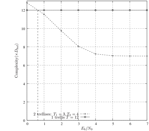
Figure 5: Computational cost of the combined trellis decoding approach versus $E_{b}/N_{0}$ against the computational cost of a single trellis decoding approach for parameters $(T_{1}=3,T_{2}=4,T_{3}=12)$. The corresponding cut-off value of $E_{b}/N_{0}$ is also depicted and is obtained for $\rho^{*}=0.417$.

IV-D Constrained optimization of trellis parameters $T_{1}$ and $T_{2}$

Let $T_{c}$ be a targeted decoding performance. According to the combined trellis decoding scheme described above, this level of performance can be reached using two trellises of parameters $T_{1}$ and $T_{2}$ such that $T_{1}\times T_{2}=T_{c}$, $T_{1}$ and $T_{2}$ being relatively prime. Without loss of generality, let us assume that $T_{2}=T_{1}+\Delta T$, and $T_{c}=T_{1}\times(T_{1}+\Delta T)$. Note that parsing the set ${\mathbb{N}}^{*}\times{\mathbb{N}}^{*}$ with the pairs $(T_{1},\Delta T)$ ensures to parse the set of attainable constraints. The probability $\rho$ is a function of $T_{1}$ and $T_{2}$, hence a function of $T_{1}$ and $\Delta T$. The computational cost $D_{mtd}$ of the combined trellis decoding algorithm of parameters $T_{1}$ and $T_{1}+\Delta T$ is given by

$$D_{\text{mtd}}(T_{1},\Delta T) =\rho(T_{1},\Delta T)D_{T_{c}}+D_{\text{bal}}(2\,T_{1}+\Delta T)$$ (49)

The quantity $\rho(T_{1},\Delta T)$ represents the probability that the trellises of parameter $T_{1}$ and $T_{1}+\Delta T$ do not provide the same estimate. This quantity can hence be assumed to increase with $\Delta T$. This assumption may not be satisfied for codes having specific synchronisation recovery properties. For example, according to section III, even values of $T$ are not appropriate for the code ${\mathcal{C}}_{13}$. Indeed, for this code, a trellis of parameter $T=2q-1,q\in{\mathbb{N}}$ provides better decoding performance than a trellis of parameter $T=2q,q\in{\mathbb{N}}$. The previous assumption is not always satisfied for this specific code. Under the assumption that $\rho(T_{1},\Delta T)$ increases with $\Delta T$, we deduce the following property from Eqn. 49.

Property 3: Let $T_{c}\in{\mathbb{N}}^{*}$ and ${\mathcal{R}}_{p}\subseteq N^{*}\times N^{*}$ be the subset of positive integers which are relatively prime. Then

$$\arg\min_{T_{1},T_{2}\in{\mathcal{R}}_{p}\ /\ T_{1}T_{2}=T_{c}}D_{\text{mtd}}=\arg\min_{T_{1},T_{2}\in{\mathcal{R}}_{p}\ /\ T_{1}T_{2}=T_{c}}|T_{2}-T_{1}|.$$ (50)

According to that property, the set of pairs $(T_{1},T_{2})$ such that $T_{2}=T_{1}+1$ is optimum.

V Conclusion

This paper makes the link between re-synchronisation properties of VLCs and length-constrained MAP estimation techniques of these codes. This analysis is also used to assess conditions for optimality of state aggregation on the bit/symbol trellis widely used for soft decoding of VLC encoded sources. Nearly optimal decoding performance can be achieved with a reduced decoding complexity with respect to the classical bit/symbol trellis. A combined trellis decoding algorithm, further reducing the decoding complexity without inducing suboptimality, is then proposed. The aggregated trellises can easily be coupled with a convolutional code or a turbo-code in an iterative structure, as done in [13], and [23].

References

• [1] T. Ferguson and J. H. Rabinowitz, “Self-synchronizing huffman codes,” IEEE Trans. Inform. Theory, vol. IT-30, no. 4, pp. 687–693, July 1984.
• [2] J. Maxted and J. Robinson, “Error recovery for variables length codes,” IEEE Trans. Inform. Theory, vol. IT-31, no. 6, pp. 794–801, Nov. 1985.
• [3] G. Zhou and Z. Zhang, “Synchronization recovery of variable length codes,” IEEE Trans. Inform. Theory, vol. 48, no. 1, pp. 219–227, Jan. 2002.
• [4] M. E. Monaco and J. M. Lawler, “Corrections and additions to ”error recovery for variable length codes”,” IEEE Trans. Inform. Theory, vol. IT-33, no. 3, pp. 454–456, May 1987.
• [5] P. F. Swaszek and P. DiCicco, “More on the error recovery for variable length codes,” IEEE Trans. Inform. Theory, vol. IT-41, no. 6, pp. 2064–2071, Nov. 1995.
• [6] B. L. Montgomery and J. Abrahams, “Synchronization of binary source codes,” IEEE Trans. Inform. Theory, vol. 32, no. 6, pp. 849–854, Nov. 1986.
• [7] M. Titchener, “Generalized t-codes: extended constructions algorithm for self-synchronising codes,” IEE proceedings, vol. 43, no. 2, pp. 122–128, June 1997.
• [8] F. Freiling, D. Jungreis, F. Théberge, and K. Zeger, “Self-synchronization of huffman codes,” in Proc. Intl. Conf. Inform. Theory, July 2003.
• [9] M. Titchener, “The synchronisation of variable length codes,” IEEE Trans. Inform. Theory, vol. 43, no. 2, pp. 683–691, Mar. 1996.
• [10] V. B. Balakirsky, “Joint source-channel coding with variable length codes,” in Proc. Intl. Conf. Inform. Theory, 1997, p.419.
• [11] A. Murad and T. Fuja, “Robust transmission of variable-length encoded sources,” in Proceedings of IEEE Wireless Communications and Networking Conference, Sept. 1999, pp. 964–968.
• [12] M. Park and D. J. Miller, “Decoding entropy-coded symbols over noisy channels using discrete hmms,” in Conf. In Information Sciences and Systems, Mar. 1998, princeton.
• [13] A. Guyader, E. Fabre, C. Guillemot, and M. Robert, “Joint source-channel turbo decoding of entropy coded sources,” IEEE J. Select. Areas Commun., vol. 19, no. 9, pp. 1680–1696, Sept. 2001.
• [14] J. Kliewer and R. Thobaben, “Iterative joint source-channel decoding of variable-length codes using residual source redundancy,” IEEE Trans. Wireless Commun., vol. 4, no. 3, pp. 919–929, May 2005.
• [15] R. Bauer and J. Hagenauer, “Iterative source-channel decoding based on a trellis representation for variable length codes,” in Proc. Intl. Conf. Inform. Theory, June 2000, p. 238.
• [16] A. Murad and T. Fuja, “Joint source-channel decoding of variable length encoded sources,” in Proc. Inform. Theory Workshop, June 1998, pp. 94–95.
• [17] M. Bystrom, S. Kaiser, and A. Kopansky, “Soft source decoding with applications,” IEEE Trans. Circuits Syst. Video Technol., vol. 11, no. 10, pp. 1108–1120, Oct. 2001.
• [18] C. Weidmann, “Reduced-complexity soft-in-soft-out decoding of variable length codes,” in Proc. Intl. Conf. Inform. Theory, July 2003, yokohama, Japan.
• [19] R. Thobaben and J. Kliewer, “Robust decoding of variable length encoded markov sources using a three-dimensional trellis,” IEEE Trans. Commun., pp. 787–794, July 2003.
• [20] H. Jegou, S. Malinowski, and C. Guillemot, “Trellis state aggregation for soft decoding of variable length codes,” in IEEE Workshop on Signal Processing Systems, Athens, Greece, Nov. 2005.
• [21] A. Viterbi, “Error bounds for convolution codes and an asymptotically optimum decoding algorithm,” IEEE Trans. Inform. Theory, no. 13, pp. 260–269, 1967.
• [22] V. Levenshtein, “Binary codes capable of correcting deletions, insertions and reversals,” Soviet Physics Doklady, vol. 10, pp. 707–710, 1966.
• [23] R. Bauer and J. Hagenauer, “Symbol by symbol map decoding of variable length codes,” in Proc. 3rd ITG Conf. Source and Channel Coding, Munich, Germany, Jan. 17.-19. 2000, 2000.