Explicit factors of some iterated resultants and discriminants

Abstract.

In this paper, the result of applying iterative univariate resultant constructions to multivariate polynomials is analyzed. We consider the input polynomials as generic polynomials of a given degree and exhibit explicit decompositions into irreducible factors of several constructions involving two times iterated univariate resultants and discriminants over the integer universal ring of coefficients of the entry polynomials. Cases involving from two to four generic polynomials and resultants or discriminants in one of their variables are treated. The decompositions into irreducible factors we get are obtained by exploiting fundamental properties of the univariate resultants and discriminants and induction on the degree of the polynomials. As a consequence, each irreducible factor can be separately and explicitly computed in terms of a certain multivariate resultant. With this approach, we also obtain as direct corollaries some results conjectured by Collins [9] and McCallum [26, 27] which correspond to the case of polynomials whose coefficients are themselves generic polynomials in other variables. Finally, a geometric interpretation of the algebraic factorization of the iterated discriminant of a single polynomial is detailled.

1. Introduction

Resultants provide an essential tool in constructive algebra and in equation solving, for projecting the solution of a polynomial system into a space of smaller dimension. In the univariate case, a well-known construction due to J.J. Sylvester (1840) consists in eliminating the monomials $1,X,\ldots,X^{m+n-1}$ in the multiples

$$(X^{i}P(X))_{0\leq i\leq n-1},(X^{j}Q(X))_{0\leq j\leq m-1},$$

of two given polynomials $P,Q$ of degree $m$ and $n$, and in taking the determinant of the corresponding $(m+n)\times(m+n)$ matrix. Though the first resultant construction appeared probably in the work of E. Bézout [4] (see also Euler’s work), and although contemporary to related works (Jacobi 1835, Richelot 1840, Cauchy 1840, …), this method remains well-known as Sylvester’s resultant. It is nowadays a fundamental tool used in effective algebra to eliminate a variable between two polynomials.

It is a natural belief that equipped with such a tool which eliminates one variable at a time, one can iteratively eliminate several variables. This approach was actually exploited, for instance in [30], to deduce theoretical results (such as the existence of eliminant polynomials) in several variables. However, if we are interested in structural results as well as practical computations or complexity issues, this approach is far from being optimal. This explains the study and development of different types of multivariate resultants, including projective [23, 18], anisotropic [18, 19], toric [14, 13, 12], residual [19, 7, 5], determinantal [8] resultants.

Nevertheless, in some algorithms, such as in Cylindrical Algebraic Decomposition (CAD), an induction is applied on the dimension of the problems and iterated univariate resultants and subresultants are used at many steps of the algorithm [9, 3]. In its original paper on quantifier elimination for real closed fields by cylindrical algebraic decomposition [9], Collins used these iterated resultants in a geometric context and observed certain intriguing factorizations that “suggest some theorems” [9, p.178]. The same year, 1975, Van der Waerden responded to these observations in a handwritten letter where he gave some intuitive hints for some of the phenomena noticed by Collins. More recently, McCallum [26, 27] proved rigorously that certain iterated resultants have some irreducible factors, but he only showed the existence and did not give a way to compute them independently. As pointed out by Jean-Pierre Jouanolou, in 1868 and 1869 Olaus Henrici published two outstanding papers [16, 17] addressing the decomposition of the discriminant of a discriminant. In particular, he gave the expected factorization of such a repeated discriminant. However, he did not prove the irreducibility of these factors which is a more difficult task. One of our goals in this paper is to give the decomposition into irreducible factors of these iterated resultant computations.

From a geometric point of view, we are interested in the solutions of equations depending on some parameters and by analyzing what happens “above”, when we move these parameters. The number of solutions might change if we cross the set of points where a vertical line is tangent to the solution set (that is to the polar variety in the vertical direction). This polar variety projected in one dimension less, might have singularities where the number of solutions changes effectively or which are only due to the superposition of distinct points of this polar variety. These critical points of the polar variety of an algebraic surface $f(x,y,z)=0$ in ${\mathbb{R}}^{3}$ are used effectively in algorithms for computing the topology of the surface (see e.g. [28]). The projection of the polar curve (say on the $(x,y)$-plane) is obtained by a discriminant computation and the critical points of this projected curve are again computed by a discriminant. These values are then used to analyze where the topology of a plane section is changing in order to deduce the topology of the whole surface $f(x,y,z)=0$. Similar projection tools are also implicitly used in higher dimension for the triangulation of hypersurfaces (see e.g. [15]), which leads in the algebraic context to univariate resultant computation (see e.g. [10, 3]).

Another of our objectives is to show how these critical points corresponding generically to folds, double folds or pleats of the surface can be related to explicit factors in iterated resultant constructions. The main results of this paper are complete explicit factorizations of two times iterated univariate resultants and discriminants of generic polynomials of given degree. We actually give the decomposition of these iterated resultants over the integer universal ring of coefficients of polynomials of given degree. Such a formulation has the advantage to allow the pre-computation of a given factor. It has direct applications to the topological computation of algebraic surfaces, which was our starting point.

Our approach is based on the study of these iterated resultants in generic situations. Most of the interesting formulas are obtained by suitable specialization of this case. These specializations are performed using the formalism of the multivariate resultant as it has been originaly introduced and deeply developed by Jouanolou to whom this paper is dedicated in recognation of its outstanding contributions to resultant theory (e.g. [18, 19, 20]). It should be noticed that this approach can be pushed further to study more particular situations (corresponding to other type of multivariate resultants) that we did not consider in this paper, but which could be interesting for specific applications.

The paper is structured as follows. In the next section, we recall the definitions and main properties of resultants and discriminants that we will use. In section 3, we consider the computation of iterated resultants of $4$ and then $3$ polynomials. In section 4, we analyze the iterated computation of resultants of discriminants, first the resultant of the discriminants of two distinct polynomials $P_{1}$, $P_{2}$ and next the resultant of the discriminant of $P_{1}$ and the resultant of $P_{1},P_{2}$. We here extend the previous work [26] and prove some properties conjectured by Collins and McCallum. In section 5, we study the discriminant of a resultant, simplifying the proof and also extending some results of [26, 27]. These developments are used in cascade to provide, in section 6, the complete factorization into irreducible components of a discriminant of a discriminant for a generic polynomial, as conjectured in [27]. These new results have direct corollaries for polynomials whose coefficients are themselves generic polynomials in other parameter variables, which we provide.

2. Background material and notation

In this section we give the notation and quickly present the tools, as resultants and discriminants, that we will use all along this paper.

2.1. Resultants

2.1.1. The univariate case

Let $\SS$ be a commutative ring (with unity) and consider the two polynomials in $\SS[X]$

$$f(X):=a_{m}X^{m}+a_{m-1}X^{m-1}+\cdots+a_{0},\ g(X):=b_{n}X^{n}+b_{n-1}X^{n-1}+\cdots+b_{0},$$

where $a_{i},b_{j}\in\SS$, and $m$ and $n$ are both positive integers. Their resultant (in degrees $m,n$) that we will denote ${\operatorname{Res}}_{X}(f,g)$, is defined as the determinant of the well-known Sylvester matrix

$$\left(\begin{array}[]{ccccccc}a_{m}&0&\cdots&0&b_{n}&0&0\\ a_{m-1}&a_{m}&&\vdots&b_{n-1}&\ddots&0\\ \vdots&&\ddots&0&\vdots&&b_{n}\\ a_{0}&&&a_{m}&b_{1}&&b_{n-1}\\ 0&a_{m}&&a_{m-1}&b_{0}&&\vdots\\ \vdots&&\ddots&\vdots&0&\ddots&b_{1}\\ 0&\cdots&0&a_{0}&0&0&b_{0}\\ \end{array}\right).$$

Remark 2.1.

We emphasize that the notation ${\operatorname{Res}}_{X}(f,g)$ denotes the resultant of $f$ and $g$ with respect to the variable $X$ as polynomials of their expected degree, which is here $m$ and $n$ respectively. It is important to keep this in mind since the closed formulas we will prove in this paper are using this convention; see Remark 3.5 for an illustration.

This “eliminant polynomial” has a long history and many known properties. One can learn about it in many places in the literature, for instance [11, 22]; see also [14, chapter 12] and [1] for a detailed exposition. In the sequel we will especially use the following properties:

• ${\operatorname{Res}}_{X}(f,g)$ belongs to the ideal $(f,g)\subset\SS[X],$

• ${\operatorname{Res}}_{X}(f,g)$ is homogeneous of degree $n$, resp. $m$, in the $a_{i}$’s, resp. in the $b_{j}$’s,

• ${\operatorname{Res}}_{X}(f,g)$ is homogeneous of degree $mn$ if we set $\deg(a_{i}):=m-i$ and $\deg(b_{j}):=n-j$ for all $i=0,\ldots,m$ and $j=0,\ldots,n$.

We also recall the definition of the principal subresultant of $f$ and $g$ that we will use later on. It is defined as the determinant of the above Sylvester matrix where the two last lines and columns number $n$ and $n+m$ are erased; more precisely

$$\mathrm{SRes}^{(1)}_{X}(f,g):=\left|\begin{array}[]{ccccccccc}a_{m}&0&\cdots&0&0&b_{n}&0&0&0\\ a_{m-1}&a_{m}&&\vdots&\vdots&b_{n-1}&\ddots&0&0\\ \vdots&a_{m-1}&\ddots&0&0&\vdots&&b_{n}&0\\ a_{2}&&\ddots&a_{m}&0&\vdots&&b_{n-1}&b_{n}\\ a_{1}&a_{2}&&a_{m-1}&a_{m}&b_{2}&&\vdots&b_{n-1}\\ a_{0}&a_{1}&\ddots&\vdots&a_{m-1}&b_{1}&&\vdots&\vdots\\ 0&\ddots&\ddots&a_{2}&\vdots&b_{0}&\ddots&b_{2}&\vdots\\ \vdots&&\ddots&a_{1}&a_{2}&0&\ddots&b_{1}&b_{2}\\ 0&\cdots&0&a_{0}&a_{1}&0&0&b_{0}&b_{1}\\ \end{array}\right|$$

(it is a square matrix of size $(m+n-2)\times(m+n-2)$). Note that the subresultants share a lot of properties with the resultants; we refer the interested reader to [1].

2.1.2. The multivariate case

All along this paper we will also use resultants of several homogeneous polynomials; we now quickly recall this notion. Although they are usually defined “geometrically” (as equations of certain hypersurfaces obtained by projection of an incidence variety), we will follow the formalism developed by Jouanolou [18] because it easily provides many properties of resultants.

Suppose given an integer $n\geq 1$, and a sequence of positive integers $d_{1},\ldots,d_{n}$. One considers the $n$ “generic” homogeneous polynomials of degree $d_{1},\ldots,d_{n}$, respectively, in the variables $X_{1},\ldots,X_{n}$ (all assumed to have weight 1) :

$$f_{i}(X_{1},\ldots,X_{n})=\sum_{|\alpha|=d_{i}}U_{i,\alpha}X^{\alpha},\ \ i=1,\ldots,n.$$

Denoting ${{\mathbb{U}}}:={\mathbb{Z}}[U_{i,\alpha}:i=1,\ldots,r,|\alpha|=d_{i}]$, the polynomials $f_{1},\ldots,f_{n}$ belongs to the ring ${C}:={{\mathbb{U}}}[X_{1},\ldots,X_{n}]$. The ideal of inertia forms of these polynomials is the ideal of ${C}$

$$\mathrm{TF}_{\mathfrak{m}}(f_{1},\ldots,f_{n}):=\{f\in{C}:\exists\nu\in\mathbb{N}\ {\mathfrak{m}}^{\nu}f\subset(f_{1},\ldots,f_{n})\}\subset{C}$$

where ${\mathfrak{m}}:=(X_{1},\ldots,X_{n})\subset C.$ It is naturally graded and it turns out that its degree zero graded part, denoted $\mathrm{TF}_{\mathfrak{m}}(f_{1},\ldots,f_{n})_{0}$, is a principal ideal of ${\mathbb{U}}$ and has a unique generator, denoted ${\operatorname{Res}}_{X_{1}:\cdots:X_{n}}$ or simply ${\operatorname{Res}}$, which satisfies

(2.1) $${\operatorname{Res}}(X_{1}^{d_{1}},\ldots,X_{n}^{d_{n}})=1.$$

To define the resultant of any given $n$-uples of homogeneous polynomials in the variables $X_{1},\ldots,X_{n}$ (and also to clarify the left side of the equality (2.1)) one proceeds as follows: Let $\SS$ be a commutative ring. For all integers $i\in\{1,\ldots,n\}$, suppose given a homogeneous polynomial of degree $d_{i}$ in the variables $X_{1},\ldots,X_{n}$

$$g_{i}=\sum_{|\alpha|=d_{i}}u_{i,\alpha}X^{\alpha}\in\SS[X_{1},\ldots,X_{n}]_{d_{i}}$$

and consider the morphism $\theta:{{\mathbb{U}}}\rightarrow\SS:U_{j,\alpha}\mapsto u_{j,\alpha}$ which corresponds to the specialization of the polynomials $f_{i}$ to the polynomials $g_{i}$. Then, given an inertia form $a\in\mathrm{TF}_{\mathfrak{m}}(f_{1},\ldots,f_{n})$ we set $a(g_{1},\ldots,g_{n}):=\theta(a).$ In particular, the resultant of $g_{1},\ldots,g_{n}$ is nothing but

$${\operatorname{Res}}(g_{1},\ldots,g_{n}):=\theta({\operatorname{Res}}(f_{1},\ldots,f_{n})).$$

Also, if $\SS={{\mathbb{U}}}$ and $\theta$ is the identity (i.e. $g_{i}=f_{i}$ for all $i$), then we get $a=a(f_{1},\ldots,f_{n})$; this clarifies the notation ${\operatorname{Res}}(f_{1},\ldots,f_{n})$ for the inertia form ${\operatorname{Res}}\in{\mathbb{U}}$.

Resultants have a lot of interesting properties. We recall the ones we will use in the sequel and refer the reader to [18, §5] for the proofs. Mention that many formulas are known to compute explicitly these resultants (e.g. [23], [20], [14], [11] and the reference therein).

Let $\SS$ be any commutative ring and suppose given $f_{1},\ldots,f_{n}$ homogeneous polynomials in the polynomial ring $\SS[X_{1},X_{2},\ldots,X_{n}]$ of positive degree $d_{1},\ldots,d_{n}$ respectively.

• homogeneity: for all $i=1,\ldots,n$, ${\operatorname{Res}}(f_{1},\ldots,f_{n})$ is homogeneous w.r.t. the coefficients of $f_{i}$ of degree $d_{1}\ldots d_{n}/d_{i}$,

• isobarity: ${\operatorname{Res}}(f_{1},\ldots,f_{n})$ is isobaric of degree $d_{1}\ldots d_{n}$ by giving to each coefficient of the $f_{i}$’s the power of its corresponding monomial in the variable $X_{n}$,

• permutation of variables:

  $${\operatorname{Res}}(f_{\sigma(1)},\ldots,f_{\sigma(n)})=(\mathcal{E}(\sigma))^{d_{1}\ldots d_{n}}{\operatorname{Res}}(f_{1},\ldots,f_{n})$$

  for any permutation $\sigma$ of the set $\{1,\ldots,n\}$ ($\mathcal{E}(\sigma)$ denotes the signature of the permutation $\sigma$),

• elementary transformations:

  $${\operatorname{Res}}(f_{1},\ldots,f_{i}+\sum_{i\neq j}h_{j}f_{j},\ldots,f_{n})={\operatorname{Res}}(f_{1},\ldots,f_{n}),$$

• multiplicativity:

  $${\operatorname{Res}}(f_{1}^{\prime}f_{1}^{\prime\prime},f_{2},\ldots,f_{n})={\operatorname{Res}}(f_{1}^{\prime},f_{2},\ldots,f_{n}){\operatorname{Res}}(f_{1}^{\prime\prime},f_{2},\ldots,f_{n})$$

• base change formula: if $g_{1},\ldots,g_{n}$ are homogeneous polynomials in $\SS[X]$ of the same positive degree $d$, then

  (2.2) $${\operatorname{Res}}(f_{1}(g_{1},\ldots,g_{n}),\ldots,f_{n}(g_{1},\ldots,g_{n}))=\\ {\operatorname{Res}}(g_{1},\ldots,g_{n})^{d_{1}\ldots d_{n}}{\operatorname{Res}}(f_{1},\ldots,f_{n})^{d^{n-1}},$$$$

• divisibility: if $g_{1},\ldots,g_{n}$ are homogeneous polynomials in $\SS[X]$ such that for all $i=1,\ldots,n$ there exists an integer $\mu_{i}$ such that $f_{i}\in(g_{1},\ldots,g_{n})^{\mu_{i}}$, then ${\operatorname{Res}}(g_{1},\ldots,g_{n})^{\mu_{1}\ldots\mu_{n}}$ divides ${\operatorname{Res}}(f_{1},\ldots,f_{n})$ in $\SS$.

In the following, we are going to consider resultant computation for eliminating a subset $X_{i_{1}},\ldots,X_{i_{k}}$ of the variables. Such a resultant, obtained by considering the homogenization of the polynomials with respect to this variable subset, will be denoted hereafter ${\operatorname{Res}}_{X_{i_{1}},\ldots,X_{i_{k}}}$. With this notation, for homogeneous polynomials $f_{1},\ldots,f_{n}\in\SS[X]$, we have

$${\operatorname{Res}}_{X_{1}:\cdots:X_{n}}(f_{1},\ldots,f_{n})={\operatorname{Res}}_{X_{2},\ldots,X_{n}}(f_{1}(1,X_{2},\ldots,X_{n}),\ldots,f_{n}(1,X_{2},\ldots,X_{n})).$$

2.2. Discriminants

Given a polynomial

$$P(X):=a_{0}X^{n}+a_{1}X^{n-1}+\cdots+a_{n-1}X+a_{n}\in\SS[X]$$

where $n\geq 1$ and $\SS$ is any commutative ring, we recall that the discriminant of $P$, denoted ${\mathrm{Disc}}_{X}(P)$, satisfies the equality

(2.3) $$a_{0}{\mathrm{Disc}}_{X}(P(X))={\operatorname{Res}}_{X}(P(X),\partial_{X}P(X))={\operatorname{Res}}_{X}(\partial_{X}P(X),P(X))$$

where $\partial_{X}$ stands for the derivative with respect to the variable $X$, i.e. $\partial/\partial_{X}$. Its properties follow immediately from the ones of the resultant. In particular, its degree in the coefficients of $P$ is $2(d-1)$. Note that in our notation the polynomial $P$ is seen as a polynomial of its expected degree, here $n$, as we did for the resultant. Indeed, in (2.3) the considered resultants are in degrees $(n,n-1)$ and $(n-1,n)$ respectively.

Given a homogeneous polynomial $P(X_{1},X_{2},X_{3})=\sum_{|\alpha|=d}U_{\alpha}X_{1}^{\alpha_{1}}X_{2}^{\alpha_{2}}X_{3}^{\alpha_{3}}$ of degree $d$, its discriminant is the polynomial in the universal ring of coefficients ${\mathbb{U}}:={\mathbb{Z}}[U_{\alpha};|\alpha|=d]$, denoted ${\mathrm{Disc}}_{X_{1}:X_{2}:X_{3}}(P)$ or simply ${\mathrm{Disc}}(P)$, which satisfies

(2.4) $$d^{d^{2}-3d+3}{\mathrm{Disc}}_{X_{1}:X_{2}:X_{3}}(P)={\operatorname{Res}}_{X_{1}:X_{2}:X_{3}}(\partial_{1}P,\partial_{2}P,\partial_{3}P)$$

where $\partial_{i}$ stands for $\partial/\partial_{X_{i}}$ for all $i$. It is an irreducible polynomial in ${\mathbb{U}}$ which is homogeneous of degree $3(d-1)^{2}$ in the $U_{\alpha}$’s. Note that we also have the following equality in ${\mathbb{U}}$:

$${\operatorname{Res}}_{X_{1}:X_{2}:X_{3}}(\partial_{1}P,\partial_{2}P,P)={\mathrm{Disc}}_{X_{1}:X_{2}:X_{3}}(P){\mathrm{Disc}}_{X_{2}:X_{3}}(P(0,X_{2},X_{3}))\\ ={\mathrm{Disc}}_{X_{1}:X_{2}:X_{3}}(P){\mathrm{Disc}}_{X_{3}}(P(0,1,X_{3})).$$

Finally, we also recall that being given two homogeneous polynomials $P_{1}$ and $P_{2}$ in the variables $X_{1},X_{2},X_{3}$ of degree $d_{1},d_{2}$ respectively, their discriminant is defined by the formula [21]

$${\mathrm{Disc}}_{X_{1}:X_{2}:X_{3}}(P_{1},P_{2})=\frac{{\operatorname{Res}}_{X_{1}:X_{2}:X_{3}}(P_{1},P_{2},\partial_{2}P_{1}\partial_{3}P_{2}-\partial_{2}P_{2}\partial_{3}P_{1})}{{\operatorname{Res}}_{X_{1}:X_{2}:X_{3}}(P_{1},P_{2},X_{1})}\in{\mathbb{U}}$$

where ${\mathbb{U}}$ denotes the universal ring of coefficients of $P_{1}$ and $P_{2}$ over ${\mathbb{Z}}$. It is an irreducible polynomial in ${\mathbb{U}}$ which is homogeneous with respect to the coefficients of $P_{1}$ of degree $d_{2}(2(d_{1}-1)+d_{2}-1)$ and homogeneous with respect to the coefficients $P_{2}$ of degree $d_{1}(2(d_{2}-1)+d_{1}-1)$.

2.3. Notations and derivatives

Let $\SS$ be a commutative ring and suppose given a polynomial $P(X)\in\SS[X]$. We denote by $\partial_{X}P$ the formal derivative of $P$ with respect to the variable $X$. More precisely, the map

$$\partial_{X}:\SS[X]\rightarrow\SS[X]:P\mapsto\partial_{X}P$$

is $\SS$-linear and for all integers $k\geq 0$ we have $\partial_{X}(X^{k})=kX^{k-1}$. For any integer $i\geq 1$ we define $\partial_{X}^{i}$ as the composition of $\partial_{X}$ with itself $i$ times; for instance $\partial_{X}^{i}(X^{k})$ is either equal to $0$ if $k<i$ or either equal to $k!/(k-i)!X^{k-i}$ if $k\geq i$.

Now, suppose given an element $a\in\SS$ and consider the $\SS$-linear map

$$\delta_{a}:\SS[X]\rightarrow\SS[X]:P\mapsto\delta_{a}P:=\frac{P(X)-P(a)}{X-a}.$$

For instance, for all integers $k\geq 1$ we have $\delta_{a}(X^{k})=\sum_{j=0}^{k-1}a^{k-1-j}X^{j}$. As above, for any integer $i\geq 1$ we define $\delta_{a}^{i}$ as the composition of $\delta_{a}$ with itself $i$ times. It follows that for all integers $n\geq 1$

(2.5) $$P(X)=P(a)+(X-a)\delta_{a}(P)(a)+(X-a)^{2}\delta_{a}^{2}(P)(a)+\cdots+(X-a)^{n}\delta_{a}^{n}(P)(X).$$

Indeed, we have $P(X)=P(a)+(X-a)\delta_{a}(P)(X)$ by definition. Applying this formula to $\delta_{a}(P)$ we deduce (2.5) for $n=2$. The general case is obtained by a similar induction.

Although $\SS$ is only assumed to be a commutative ring, we still have the expected formula

Lemma 2.2.

For $k\geq 1$, for any $P\in\SS[X]$ and $a\in\SS$, we have the equality $k!\,\delta_{a}^{k}P(a)=\partial_{X}^{k}P(a)$ in $\SS$.

Proof.

Notice that $\delta_{a}P(X)$ is of degree $\deg(P)-1$ in the variable $X$. Thus if $d>\deg(P)$, we have $\delta^{d}_{a}(P)=0$. We deduce that for any polynomial $P\in\SS[X]$,

$$P(X)=P(a)+(X-a)\delta_{a}(P)(a)+\cdots+(X-a)^{d}\delta_{a}^{\deg(P)}(P)(a).$$

By the binomial identity, for any $n\in{\mathbb{N}}$, $X^{n}=\sum_{i=0}^{n}\binom{n}{k}a^{n-k}(X-a)^{k}$. By identification of the coefficients in the basis $(X-a)^{k}$ of $\SS[X]$, we deduce that for all $k\leq n$, we have $\delta_{a}^{k}(X^{n})(a)=\binom{n}{k}a^{n-k}$. As we have $\partial_{X}^{k}(X^{n})=\frac{n!}{(n-k)!}X^{n-k}$, we deduce that for any $k,n\in{\mathbb{N}}$, $k!\,\delta_{a}^{k}(X^{n})(a)=\partial_{X}^{k}(X^{n})(a)$. By linearity, we also have this identity for any polynomial $P\in\SS[X]$. ∎

As a consequence, if $\SS$ is assumed to be a $\mathbb{Q}$-algebra then (2.5) shows that for all integers $n\geq 1$

$$P(X)=P(a)+(X-a)\partial_{X}P(a)+\cdots+(X-a)^{n}\frac{\partial_{X}^{n}P(a)}{n!}+(X-a)^{n+1}\delta_{a}^{n+1}(P).$$

If $n$ is bigger than the degree of $P$, then we get the Taylor expansion formula

$$P(X)=P(a)+\sum_{n\geq 1}\frac{\partial_{X}^{n}P(a)}{n!}(X-a)^{n}.$$

We now fix a notation that we will use all along the paper. We will mainly manipulate polynomials in the three variables $X_{1},X_{2}$ and $X_{3}$ over a commutative ring $\SS$. Introducing a new indeterminate $X_{4}$, for any polynomial $P\in\SS[X_{1},X_{2},X_{3}]$ we set

$$\delta_{3,4}(P):=\frac{P(X_{1},X_{2},X_{3})-P(X_{1},X_{2},X_{4})}{X_{3}-X_{4}}\in\SS[X_{1},X_{2},X_{3},X_{4}]$$

so that we have

$$P(X_{1},X_{2},X_{4})=P(X_{1},X_{2},X_{3})+(X_{4}-X_{3})\delta_{3,4}(P).$$

Observe that $\delta_{3,4}(P)$ is nothing but $\delta_{X_{4}}(P)\in(\SS[X_{1},X_{2},X_{4}])[X_{3}]$ and therefore that all the above definitions and formulas can be expressed with this notation. Therefore, we have

(2.6) $$\delta_{3,4}P =\partial_{3}P(X_{3})+(X_{4}-X_{3})\delta_{3,4}^{2}P,$$

(2.7) $$2\delta^{2}_{3,4}P=\partial^{2}_{3}P(X_{3})+2(X_{4}-X_{3})\delta_{3,4}^{3}P\\ =\frac{2}{(X_{4}-X_{3})^{2}}\left(P(X_{1},X_{2},X_{3})-P(X_{1},X_{2},X_{4})-(X_{4}-X_{3})\partial_{3}P_{1}(X_{1},X_{2},X_{3})\right).$$

The above definition can be extended to any variable. We denote by $\delta^{2}_{i,j}$ the corresponding operation, $X_{i}$ playing the role of $X_{3}$, and $X_{j}$ the role of $X_{4}$. If the indices $i,j$ are omitted, we implicitly refer to the variables $X_{3}$ and $X_{4}$. Notice that $\delta_{3,4}P_{|X_{4}=X_{3}}=\partial_{3}P(X_{3})$. Also, by convention we set $\delta_{i,i}P=\partial_{i}P$.

We will need the two following properties: for any polynomials $L,Q$, we have

(2.8) $$\delta_{3,4}(L\,Q) = \delta_{3,4}(L)\,Q(X_{3})+L(X_{4})\,\delta_{3,4}(Q),$$

(2.9) $$\delta_{3,4}^{2}(L\,Q) = \delta_{3,4}^{2}(L)\,Q(X_{3})+\delta_{3,4}(L)\,\partial_{3}(Q)(X_{3})+L(X_{4})\,\delta_{3,4}^{2}(Q).$$

To prove (2.8), we remark that

$$L(X_{3})Q(X_{3})-L(X_{4})Q(X_{4})=Q(X_{3})(L(X_{4})-L(X_{3}))+L(X_{4})(Q(X_{4})-Q(X_{3}))$$

and divide by $(X_{4}-X_{3})$ to get the formula. To prove (2.9), we substitute (2.6) in the previous relation and obtain

$$(X_{4}-X_{3})\partial_{3}(LQ)+(X_{4}-X_{3})^{2}\delta_{3,4}^{2}(QL)\\ =(X_{4}-X_{3})(\partial_{3}(L)Q(X_{3})+L(X_{3})\,\partial_{3}(Q))+(X_{4}-X_{3})^{2}\delta_{3,4}^{2}(QL)\\ =Q(X_{3})\left((X_{4}-X_{3})\partial_{3}(L)+(X_{4}-X_{3})^{2}\delta_{3,4}^{2}(L)\right)+L(X_{4})\left((X_{4}-X_{3})\,\partial_{3}(Q)\right.\\ \left.+(X_{4}-X_{3})^{2}\delta_{3,4}^{2}(Q)\right)$$

so that

$$(X_{4}-X_{3})^{2}\delta_{3,4}^{2}(QL)=(X_{4}-X_{3})^{2}\delta_{3,4}^{2}(L)Q(X_{3})\\ +(X_{4}-X_{3})(L(X_{4})-L(X_{3}))\,\partial_{3}(Q)+(X_{4}-X_{3})^{2}\,L(X_{4})\,\delta_{3,4}^{2}(Q),$$

from which we deduce the relation (2.9).

Finally, mention that if $\SS$ is assumed to be a $\mathbb{Q}$-algebra then we have

$$P(X_{1},X_{2},X_{4})=P(X_{1},X_{2},X_{3})+(X_{4}-X_{3})\partial_{3}P(X_{3})+\cdots+\\ \frac{1}{(i-1)!}\,(X_{4}-X_{3})^{i-1}\partial_{3}^{i-1}P(X_{3})+(X_{4}-X_{3})^{i}\delta_{3,4}^{i}P$$

or equivalently $\delta_{3,4}^{i}P=\sum_{k\geq i}\frac{1}{k!}(X_{4}-X_{3})^{k-1}\partial_{3}^{k}P(X_{3}).$ Similarly, we have

(2.10) $$\delta_{3,4}^{i}P_{|X_{4}=X_{3}}=\frac{1}{i!}\partial^{i}_{3}P.$$

Notice that we will very often omit variables $X_{1}$ and $X_{2}$ in the sequel, especially in the proofs to avoid to overload the computations and the text.

2.4. A Bertini’s lemma

The elimination of the variables $X_{1},X_{2},X_{3},X_{4}$ between polynomials constructed from the polynomials

$$P_{k}(X_{1},X_{2},X_{3}):=\sum_{0\leq i,j;i+j\leq d_{k}} U^{(k)}_{i,j}X_{1}^{i}X_{2}^{j}X_{3}^{d_{k}-i-j}\in{\mathbb{U}}[X_{1},X_{2},X_{3}],$$

$k=1,\ldots,r$, where ${\mathbb{U}}$ denotes the universal coefficients ring ${\mathbb{U}}:=\mathbbm{Z}[U^{(k)}_{i,j};0\leq i,j;i+j\leq d_{k},k=1,\ldots,r]$, yields polynomials in ${\mathbb{U}}$ for which we are going to give irreducible factorizations. As in geometric applications, this computation is applied with the coefficients $U^{(k)}_{i,j}$ replaced by generic polynomials $\sum_{|\alpha|\leq d_{k}-i-j}a^{(k)}_{i,j,\alpha}\boldsymbol{x}^{\alpha}$ of degree $d_{k}-i-j\geqslant 0$, where we consider the coefficients $a^{(k)}_{i,j,\alpha}$ as indeterminates where $\boldsymbol{x}$ denotes a set of indeterminates $(x_{1},\ldots,x_{t})$ with $t\geq 1$. Therefore, we will need several times the following lemma:

Lemma 2.3.

Suppose that $R$ is an irreducible homogeneous polynomial of ${\mathbb{U}}$. Then the polynomial $R(\boldsymbol{x},\boldsymbol{a})$ obtained by substituting the coefficients $U^{(k)}_{i,j}$ by generic polynomials $\sum_{|\alpha|\leq d_{k}-i-j}a^{(k)}_{i,j,\alpha}\boldsymbol{x}^{\alpha}$ is irreducible in $\mathbbm{Z}[\boldsymbol{x},a^{(k)}_{i,j,\alpha}]$.

Proof.

Assume that $R$ is not irreducible and can be splitted into the product of two factors in $\mathbbm{Z}[\boldsymbol{x},a^{(k)}_{i,j,\alpha}]$:

$$R(a^{(k)}_{i,j,\alpha},\boldsymbol{x})=R_{1}(a^{(k)}_{i,j,\alpha},\boldsymbol{x})R_{2}(a^{(k)}_{i,j,\alpha},\boldsymbol{x}).$$

By sending $\boldsymbol{x}$ to $\boldsymbol{0}$ we observe that $R(a^{(k)}_{i,j,\alpha},\boldsymbol{0})$ is an irreducible polynomial in the $a^{(k)}_{i,j,\alpha}$ since $R$ is irreducible so that we only have to rename each coefficient $a^{(k)}_{i,j,(0,\ldots,0)}$ by $U^{(k)}_{i,j}$. It follows that either $R_{1}(a^{(k)}_{i,j,\alpha},\boldsymbol{0})$ or $R_{2}(a^{(k)}_{i,j,\alpha},\boldsymbol{0})$ must be an invertible element in $\mathbbm{Z}$. But since $R_{1}$ and $R_{2}$ are homogeneous in the coefficients $a^{(k)}_{i,j,\alpha}$ this implies that either $R_{1}$ or $R_{2}$ is an invertible element in $\mathbbm{Z}$. ∎

3. Resultant of resultants

In all this section, we suppose given four positive integers $d_{1},d_{2},d_{3},d_{4}$ and four homogeneous polynomials

$$P_{k}(X_{1},X_{2},X_{3})=\sum_{0\leq i,j;i+j\leq d_{k}}U^{(k)}_{i,j}X_{1}^{i}X_{2}^{j}X_{3}^{d_{k}-i-j}\in{\mathbb{U}}[X_{1},X_{2},X_{3}],k=1,\ldots,4,$$

where ${\mathbb{U}}$ denotes the universal ring of coefficients

$${\mathbb{U}}:=\mathbbm{Z}[U^{(k)}_{i,j};0\leq i,j;i+j\leq d_{k},k=1,\ldots,4].$$

We denote by $X_{4}$ a new indeterminate. Our first result is the most general situation of an iterated resultant with four different polynomials.

Theorem 3.1.

Defining

$$R_{12} := {\operatorname{Res}}_{X_{3}}(P_{1}(1,X_{2},X_{3}),P_{2}(1,X_{2},X_{3}))\in{\mathbb{U}}[X_{2}],$$

$$R_{34} := {\operatorname{Res}}_{X_{3}}(P_{3}(1,X_{2},X_{3}),P_{4}(1,X_{2},X_{3}))\in{\mathbb{U}}[X_{2}],$$

we have the following equality in ${\mathbb{U}}$:

$${\operatorname{Res}}_{X_{2}}(R_{12},R_{34})=\\ {\operatorname{Res}}_{X_{1}:\cdots:X_{4}}(P_{1}(X_{1},X_{2},X_{3}),P_{2}(X_{1},X_{2},X_{3}),P_{3}(X_{1},X_{2},X_{4}),P_{4}(X_{1},X_{2},X_{4})).$$

Moreover, the above quantity is non-zero, irreducible and multi-homogeneous with respect to the set of coefficients $(U^{(1)}_{i,j})_{i,j}$, $(U^{(2)}_{i,j})_{i,j}$, $(U^{(3)}_{i,j})_{i,j}$, $(U^{(4)}_{i,j})_{i,j}$ of multi-degree $(d_{2}d_{3}d_{4},d_{1}d_{3}d_{4},d_{1}d_{2}d_{4},d_{1}d_{2}d_{3}).$

Proof.

First of all, we observe that the iterated resultant ${\operatorname{Res}}_{X_{2}}(R_{12},R_{34})$ and the resultant

$$\mathcal{R}:={\operatorname{Res}}(P_{1}(X_{1},X_{2},X_{3}),P_{2}(X_{1},X_{2},X_{3}),P_{3}(X_{1},X_{2},X_{4}),P_{4}(X_{1},X_{2},X_{4}))$$

are both non-zero polynomials, for they both specialize to the quantity $(-1)^{d_{1}d_{2}d_{3}d_{4}}$ if the polynomials $P_{i}(X_{1},X_{2},X_{3}),i=1,\ldots,4,$ are specialized to $X_{1}^{d_{1}}$, $X_{3}^{d_{2}}$, $X_{2}^{d_{3}}$ and $X_{3}^{d_{4}}$ respectively. Note also that the statement about the multi-degree of $\mathcal{R}$ follows from the homogeneity property of resultants.

To prove the irreducibility of $\mathcal{R}$, we proceed by induction on the positive integer $d:=d_{1}+d_{2}+d_{3}+d_{4}\geq 4$. For $d=4$, $\mathcal{R}$ equals the determinant

$$\left|\begin{array}[]{cccc}U^{(1)}_{1,0}&U^{(2)}_{1,0}&U^{(3)}_{1,0}&U^{(4)}_{1,0}\\ U^{(1)}_{0,1}&U^{(2)}_{0,1}&0&0\\ U^{(1)}_{0,0}&U^{(2)}_{0,0}&U^{(3)}_{0,0}&U^{(4)}_{0,0}\\ 0&0&U^{(3)}_{0,1}&U^{(4)}_{0,1}\end{array}\right|\in {\mathbb{U}}$$

which is checked to be irreducible. Thus, we assume that $\mathcal{R}$ is irreducible up to a given integer $p\geq 4$ and we will prove that ${\mathcal{R}}$ is irreducible if $d=p+1$. To do this, first observe that one of the integers $d_{1},d_{2},d_{3},d_{4}$ must be greater or equal to 2. We can assume that $d_{1}\geq 2$ without loss of generality. Consider the specialization $\phi$ leaving invariant the polynomials $P_{2},P_{3}$ and $P_{4}$ and sending the polynomial $P_{1}$ to the product $L_{1}Q_{1}$ where $L_{1}$ and $Q_{1}$ are both generic forms of respective degree 1 and $d_{1}-1\geq 1$. Then, by multiplicativity of resultants we have the equality

$$\phi(\mathcal{R})={\operatorname{Res}}(L_{1},P_{2},P_{3},P_{4}){\operatorname{Res}}(Q_{1},P_{2},P_{3},P_{4}),$$

whose right hand side is a product of two irreducible polynomials by our induction hypothesis. As the specialization $\phi$ is homogeneous (in terms of the coefficients of the $P_{i}$’s, $L_{1}$ and $Q_{1}$), the number of irreducible factors of $\mathcal{R}$ can not decrease under the specialization $\phi$ and we deduce that $\mathcal{R}$ is the product of two irreducible polynomials ${\mathcal{R}}_{1}$ and ${\mathcal{R}}_{2}$. But then, one of these two factors must depend on the coefficients of $P_{1}$, say ${\mathcal{R}}_{1}$, and therefore $\phi({\mathcal{R}}_{1})$ must depend on the coefficients of $L_{1}$ and $Q_{1}$. This implies that ${\mathcal{R}}_{2}$ is an invertible element in $\mathbbm{Z}$ and consequently that $\mathcal{R}$ is irreducible.

It remains to prove the claimed equality. To do this, we rewrite $P_{k}(1,X_{2},X_{3})$, for all $k=1,\ldots,4$, as

$$P_{k}(1,X_{2},X_{3})=\sum_{i=0}^{d_{k}}\left(\sum_{j=0}^{d_{k}-i}U^{(k)}_{i,j}X_{2}^{j}\right)X_{3}^{i}\in{\mathbb{U}}[X_{2},X_{3}],$$

and we then easily see from well-known properties of the Sylvester resultant that

• $R_{12}$ is bi-homogeneous in the set of coefficients $(U^{(1)}_{i,j})$ and ($U^{(2)}_{i,j}$) of bi-degree $(d_{2},d_{1})$,

• $R_{12}$ is a polynomial $\operatorname{in}{\mathbb{U}}[X_{2}]$ of degree $d_{1}d_{2}$,

• $R_{12}\in(P_{1}(1,X_{2},X_{3}),P_{2}(1,X_{2},X_{3}))\subset{\mathbb{U}}[X_{2},X_{3}]$.

Of course, completely analogous results hold for $R_{34}$, in particular

$$R_{34}\in(P_{3}(1,X_{2},X_{4}),P_{4}(1,X_{2},X_{4}))\subset{\mathbb{U}}[X_{2},X_{4}].$$

Again, ${\operatorname{Res}}_{X_{2}}(R_{12},R_{34})\in(R_{12},R_{34})\subset{\mathbb{U}}[X_{2}]$ and we deduce that

$${\operatorname{Res}}_{X_{2}}(R_{12},R_{34})\in\\ (P_{1}(1,X_{2},X_{3}),P_{2}(1,X_{2},X_{3}),P_{3}(1,X_{2},X_{4}),P_{4}(1,X_{2},X_{4}))\subset{\mathbb{U}}[X_{2},X_{3},X_{4}].$$

After homogenization with the variable $X_{1}$, it follows that there exists an integer $N$ such that

$$X_{1}^{N}{\operatorname{Res}}_{X_{2}}(R_{12},R_{34})\in\\ (P_{1}(X_{1},X_{2},X_{3}),P_{2}(X_{1},X_{2},X_{3}),P_{3}(X_{1},X_{2},X_{4}),P_{4}(X_{1},X_{2},X_{4}))$$

in ${\mathbb{U}}[X_{1},X_{2},X_{3},X_{4}]$ (notice that this does not imply directly that ${\operatorname{Res}}_{X_{2}}(R_{12},R_{34})$ is an inertia form because $P_{1}(X_{1},X_{2},X_{3})$, $P_{2}(X_{1},X_{2},X_{3})$, $P_{3}(X_{1},X_{2},X_{4})$ and $P_{4}(X_{1},X_{2},X_{4})$ are not generic polynomials). It implies by the divisibility property of resultants, that ${\mathcal{R}}={\operatorname{Res}}(P_{1}(X_{3}),P_{2}(X_{3}),P_{3}(X_{4}),P_{4}(X_{4}))$ divides the quantity

$${\operatorname{Res}}(X_{1}^{N}{\operatorname{Res}}_{X_{2}}(R_{12},R_{34}),P_{1}(X_{1},X_{2},X_{3}),P_{2}(X_{1},X_{2},X_{3}),P_{3}(X_{1},X_{2},X_{4}))=\\ {\operatorname{Res}}_{X_{2}}(R_{12},R_{34})^{d_{1}d_{2}d_{3}}{\operatorname{Res}}(X_{1},P_{1}(X_{3}),P_{2}(X_{3}),P_{3}(X_{4}))^{N}.$$

Since $\mathcal{R}$ is irreducible and since the second term in the right hand side of the above product does not depend on the coefficients of $P_{4}$, we deduce that $\mathcal{R}$ divides ${\operatorname{Res}}_{X_{2}}(R_{12},R_{34})$. Now, from the degree properties of $R_{12}$ and $R_{13}$ we deduce that ${\operatorname{Res}}_{X_{2}}(R_{12},R_{34})$ is, similarly to $\mathcal{R}$, multi-homogeneous with respect to the set of coefficients $(U^{(1)}_{i,j})_{i,j},(U^{(2)}_{i,j})_{i,j},(U^{(3)}_{i,j})_{i,j},$ $(U^{(4)}_{i,j})_{i,j}$ of multi-degree

$$(d_{2}d_{3}d_{4},d_{1}d_{3}d_{4},d_{1}d_{2}d_{4},d_{1}d_{2}d_{3}).$$

This shows that ${\operatorname{Res}}_{X_{2}}(R_{12},R_{34})$ and $\mathcal{R}$ are equal up to multiplication by an invertible element in $\mathbbm{Z}$. To determine this invertible element, we take again the specialization sending $P_{1}$ to $X_{1}^{d_{1}}$, $P_{2}$ to $X_{3}^{d_{2}}$, $P_{3}$ to $X_{2}^{d_{3}}$, $P_{4}$ to $X_{3}^{d_{4}}$, and check that $\mathcal{R}$ specializes to $(-1)^{d_{1}d_{2}d_{3}d_{4}}$, as well as ${\operatorname{Res}}_{X_{2}}(R_{12},R_{34}).$ ∎

A specialization of this theorem gives the following result.

Corollary 3.2.

Given four polynomials $f_{k}(\boldsymbol{x},y,z),k=1,\ldots,4$, of the form

$$f_{k}(\boldsymbol{x},y,z)=\sum_{|\alpha|+i+j\leqslant d_{k}}a^{(k)}_{\alpha,i,j}\boldsymbol{x}^{\alpha}y^{i}z^{j}\in\SS[\boldsymbol{x}][y,z],$$

where $\boldsymbol{x}$ denotes a set of variables $(x_{1},\ldots,x_{n})$ for some integer $n\geq 1$ and $\SS$ is any commutative ring, then the iterated resultant ${\operatorname{Res}}_{y}({\operatorname{Res}}_{z}(f_{1},f_{2}),{\operatorname{Res}}_{z}(f_{3},f_{4}))\in\SS[\boldsymbol{x}]$ is of degree at most $d_{1}d_{2}d_{3}d_{4}$ in $\boldsymbol{x}$ and we have

$${\operatorname{Res}}_{y}({\operatorname{Res}}_{z}(f_{1},f_{2}),{\operatorname{Res}}_{z}(f_{3},f_{4}))=\\ {\operatorname{Res}}_{y,z,z^{\prime}}(f_{1}(\boldsymbol{x},y,z),f_{2}(\boldsymbol{x},y,z),f_{3}(\boldsymbol{x},y,z^{\prime}),f_{4}(\boldsymbol{x},y,z^{\prime}))\in\SS[\boldsymbol{x}].$$

Moreover, if the polynomials $f_{1},f_{2},f_{3}$ and $f_{4}$ are sufficiently generic then this iterated resultant is irreducible and has exactly degree $d_{1}d_{2}d_{3}d_{4}$ in $\boldsymbol{x}$.

Proof.

It is a corollary of Theorem 3.1. Indeed, the claimed equality is deduced from the equality given in Theorem 3.1 by substituting $X_{2}\operatorname{by}y,X_{3}\operatorname{by}z$, by seeing $X_{1}$ as the homogenization variable of the variables $(X_{2},X_{3})$ and by specializing each coefficient $U^{(k)}_{i,j}$ to $\sum_{|\alpha|\leq d_{k}-i-j}a^{(k)}_{i,j,\alpha}\boldsymbol{x}^{\alpha}$. Moreover, since each coefficient $U^{(k)}_{i,j}$ is specialized to a polynomial in $\boldsymbol{x}$ of degree at most $d_{k}$ we deduce the claimed degree bound as a consequence of the isobarity formula for resultants.

If the polynomials $f_{1},f_{2},f_{3}$ and $f_{4}$ are sufficiently generic then it is clear that the degree bound is reached: this and the irreducibility statement is a consequence of Lemma 2.3. ∎

The formula proved in Theorem 3.1 can be specialized to get the factorization of an iterated resultant which may occur quite often in practical situations (implicitization of a rational surface, projection of the intersection of two surfaces in projective space,… e.g. [24, 6]).

Proposition 3.3.

Assume that $d_{1}\geq 2$ and set

$$R_{12} := {\operatorname{Res}}_{X_{3}}(P_{1}(1,X_{2},X_{3}),P_{2}(1,X_{2},X_{3}))\in{\mathbb{U}}[X_{2}],$$

$$R_{13} := {\operatorname{Res}}_{X_{3}}(P_{1}(1,X_{2},X_{3}),P_{3}(1,X_{2},X_{3}))\in{\mathbb{U}}[X_{2}].$$

Then, we have the equality

$${\operatorname{Res}}_{X_{2}}(R_{13},R_{12})={\operatorname{Res}}_{X_{1}:X_{2}:X_{3}}(P_{1},P_{2},P_{3})\times\\ {\operatorname{Res}}_{X_{1}:\cdots:X_{4}}(P_{1}(X_{3}),P_{2}(X_{4}),P_{3}(X_{3}),\delta_{3,4}P_{1}(X_{3},X_{4}))$$

where the right hand side is a product of two irreducible polynomials in ${\mathbb{U}}$.

Moreover, the iterated resultant ${\operatorname{Res}}_{X_{2}}(R_{13},R_{12})$ is multi-homogeneous with respect to the set of coefficients $(U^{(1)}_{i,j})_{i,j},(U^{(2)}_{i,j})_{i,j},(U^{(3)}_{i,j})_{i,j}$ of degree $2d_{1}d_{2}d_{3},d_{1}^{2}d_{3}$ and $d_{1}^{2}d_{2}$ respectively.

Proof.

The claimed equality is easily obtained using formal properties of resultants by specialization of the formula proved in Theorem 3.1:

$${\operatorname{Res}}(P_{1}(X_{3}),P_{3}(X_{3}),P_{1}(X_{4}),P_{2}(X_{4}))$$

$$= {\operatorname{Res}}(P_{1}(X_{3}),P_{2}(X_{4}),P_{3}(X_{3}),P_{1}(X_{4}))$$

$$= {\operatorname{Res}}(P_{1}(X_{3}),P_{2}(X_{4}),P_{3}(X_{3}),P_{1}(X_{4})-P_{1}(X_{3}))$$

$$= {\operatorname{Res}}(P_{1}(X_{3}),P_{2}(X_{4}),P_{3}(X_{3}),(X_{4}-X_{3})\delta_{3,4}(P_{1}))$$

$$= {\operatorname{Res}}(P_{1},P_{2},P_{3}){\operatorname{Res}}(P_{1}(X_{3}),P_{2}(X_{4}),P_{3}(X_{3}),\delta_{3,4}(P_{1})).$$

The multi-degree computation and the irreducibility of ${\operatorname{Res}}(P_{1},P_{2},P_{3})$ are known properties of resultants. The only point which requires a proof is the irreducibility of the factor (which is easily seen to be non-zero by a straightforward specialization)

$$\mathcal{D}:={\operatorname{Res}}(P_{1}(X_{3}),P_{2}(X_{4}),P_{3}(X_{3}),\delta_{3,4}(P_{1})(X_{3},X_{4})).$$

To do this, we proceed similarly to what we did in Theorem 3.1, that is, by induction on the integer $d:=d_{1}+d_{2}+d_{3}\geq 4$. We can check by hand (or with a computer) that $\mathcal{D}$ is an irreducible polynomial in ${\mathbb{U}}$ if $(d_{1},d_{2},d_{3})=(2,1,1).$  We thus assume that $\mathcal{D}$ is irreducible up to a given integer $p\geq 4$ and we will prove that $\mathcal{D}$ is irreducible if $d=p+1$. If $d_{2}\geq 2$ (resp. $d_{3}\geq 2$) then we can specialize $P_{2}$ (resp. $P_{3}$) as a product of a generic linear form and a generic form of degree $d_{2}-1\geq 1$ (resp. $d_{3}-1\geq 1$) and conclude, exactly as we did in Theorem 3.1, that $\mathcal{D}$ is then irreducible. Otherwise, then $d_{1}\geq 3$ and we specialize $P_{1}$ to the product of a generic linear form

$$L_{1}(X_{1},X_{2},X_{3}):=a\,X_{1}+b\,X_{2}+c\,X_{3}$$

and a generic form $Q_{1}$ of degree $d_{1}-1\geq 2$. We call $\phi$ the map corresponding to this specialization. By (2.8), we have

$$\delta_{3,4}(L_{1}Q_{1})(X_{3},X_{4})=c\,Q_{1}(X_{3})+L_{1}(X_{4})\,\delta_{3,4}(Q_{1})(X_{3},X_{4})$$

and we deduce after some manipulations on resultants that

$$\phi(\mathcal{D}) = {\operatorname{Res}}(L_{1}(X_{3})Q_{1}(X_{3}),P_{2}(X_{4}),P_{3}(X_{3}),cQ_{1}(X_{3})+L_{1}(X_{4})\delta_{3,4}(Q_{1}))$$

$$= {\operatorname{Res}}(Q_{1}(X_{3}),P_{2}(X_{4}),P_{3}(X_{3}),L_{1}(X_{4})\delta_{3,4}(Q_{1})(X_{3},X_{4}))\times$$

$${\operatorname{Res}}(L_{1}(X_{3}),P_{2}(X_{4}),P_{3}(X_{3}),cQ_{1}(X_{3})+L_{1}(X_{4})\delta_{3,4}(Q_{1})(X_{3},X_{4}))$$

$$= {\operatorname{Res}}(Q_{1}(X_{3}),P_{2}(X_{4}),P_{3}(X_{3}),\delta_{3,4}(Q_{1})(X_{3},X_{4}))\times$$

$${\operatorname{Res}}(Q_{1}(X_{3}),P_{2}(X_{4}),P_{3}(X_{3}),L_{1}(X_{4}))\times$$

$${\operatorname{Res}}(L_{1}(X_{3}),P_{2}(X_{4}),P_{3}(X_{3}),(L_{1}(X_{4})-L_{1}(X_{3}))\delta_{3,4}(Q_{1})+cQ_{1}(X_{3}))$$

$$= {\operatorname{Res}}(Q_{1}(X_{3}),P_{2}(X_{4}),P_{3}(X_{3}),\delta_{3,4}(Q_{1})(X_{3},X_{4}))\times$$

$${\operatorname{Res}}(Q_{1}(X_{3}),P_{2}(X_{4}),P_{3}(X_{3}),L_{1}(X_{4}))\times$$

$${\operatorname{Res}}(L_{1}(X_{3}),P_{2}(X_{4}),P_{3}(X_{3}),cQ_{1}(X_{4}))$$

$$= c^{d_{2}d_{3}}Res(Q_{1}(X_{3}),P_{2}(X_{4}),P_{3}(X_{3}),\delta_{3,4}(Q_{1})(X_{3},X_{4}))\times$$

$${\operatorname{Res}}(Q_{1}(X_{3}),P_{2}(X_{4}),P_{3}(X_{3}),L_{1}(X_{4}))\times$$

$${\operatorname{Res}}(L_{1}(X_{3}),P_{2}(X_{4}),P_{3}(X_{3}),Q_{1}(X_{4})).$$

Either by our induction hypothesis or by Theorem 3.1, it turns out that the three resultants involved in the right hand side of the above computation are irreducible in ${\mathbb{U}}$. So if $\mathcal{D}$ were reducible, say $\mathcal{D}=\mathcal{D}_{1}\mathcal{D}_{2}$, then each factor should be homogeneous in the coefficients $(U_{i,j}^{(1)})_{i,j}$ and hence $\phi(\mathcal{D}_{1})$ and $\phi(\mathcal{D}_{2})$ should be homogeneous in the coefficients of $Q_{1}$ and $L_{1}$ of the same degree. But

$$\deg_{L_{1},Q_{1}}(c) =(1,0),$$

$$\deg_{L_{1},Q_{1}}\left({\operatorname{Res}}(L_{1}(X_{3}),P_{2}(X_{4}),P_{3}(X_{3}),Q_{1}(X_{4}))\right) =((d_{1}-1)d_{2}d_{3},d_{2}d_{3}),$$

$$\deg_{L_{1},Q_{1}}\left({\operatorname{Res}}(Q_{1}(X_{3}),P_{2}(X_{4}),P_{3}(X_{3}),L_{1}(X_{4}))\right) =((d_{1}-1)d_{2}d_{3},d_{2}d_{3}),$$

$$\deg_{L_{1},Q_{1}}\left({\operatorname{Res}}(Q_{1}(X_{3}),P_{2}(X_{4}),P_{3}(X_{3}),\delta_{3,4}(Q_{1})(X_{3},X_{4}))\right) =(0,2d_{1}d_{2}d_{3}-3d_{2}d_{3}),$$

which implies that either $\mathcal{D}_{1}$ or $\mathcal{D}_{2}$ is an invertible element in $\mathbbm{Z}$. ∎

As a consequence of this proposition, we get the following result which improves Theorem 3.1 and Theorem 3.2 in [26].

Corollary 3.4.

Given three polynomials $f_{k}(\boldsymbol{x},y,z),k=1,\ldots,3$, of the form

$$f_{k}(\boldsymbol{x},y,z)=\sum_{|\alpha|+i+j\leqslant d_{k}}a^{(k)}_{\alpha,i,j}\boldsymbol{x}^{\alpha}y^{i}z^{j}\in\SS[\boldsymbol{x}][y,z],$$

where $\boldsymbol{x}$ denotes a set of variables $(x_{1},\ldots,x_{n})$ for some integer $n\geq 1$ and $\SS$ is any commutative ring, then the iterated resultant ${\operatorname{Res}}_{y}({\operatorname{Res}}_{z}(f_{1},f_{2}),{\operatorname{Res}}_{z}(f_{1},f_{3}))\in\SS[\boldsymbol{x}]$ is of degree at most $d_{1}^{2}d_{2}d_{3}$ in $\boldsymbol{x}$ and we have

$${\operatorname{Res}}_{y}({\operatorname{Res}}_{z}(f_{1},f_{2}),{\operatorname{Res}}_{z}(f_{1},f_{3}))=(-1)^{d_{1}d_{2}d_{3}}\times\\ {\operatorname{Res}}_{y,z}(f_{1}(\boldsymbol{x},y,z),f_{2}(\boldsymbol{x},y,z),f_{3}(\boldsymbol{x},y,z))\times\\ {\operatorname{Res}}_{y,z,z^{\prime}}(f_{1}(\boldsymbol{x},y,z),f_{2}(\boldsymbol{x},y,z),f_{3}(\boldsymbol{x},y,z^{\prime}),\delta_{z,z^{\prime}}(f_{1})).$$

Moreover, if the polynomials $f_{1},f_{2},f_{3}$ are sufficiently generic then this iterated resultant has exactly degree $d_{1}^{2}d_{2}d_{3}$ in $\boldsymbol{x}$ and both resultants on the right hand side of the above equality are distinct and irreducible.

This corollary can be interpreted geometrically as follows. For simplicity we assume that $\boldsymbol{x}$ is a unique variable $x$ and that $f_{1}$, $f_{2}$ and $f_{3}$ are three polynomial in $x,y,z$. The resultant $R_{12}:={\operatorname{Res}}_{z}(f_{1},f_{2})$ defines the projection of the intersection curve between the two surfaces $\{f_{1}=0\}$ and $\{f_{2}=0\}$. Similarly, $R_{13}:={\operatorname{Res}}_{z}(f_{1},f_{3})$ defines the projection of the intersection curve between the two surfaces $\{f_{1}=0\}$ and $\{f_{3}=0\}$. Then the roots of ${\operatorname{Res}}_{y}(R_{12},R_{13})$ can be decomposed into two distinct sets: the set of roots $x_{0}$ such that there exists $y_{0}$ and $z_{0}$ such that $f_{1}(x_{0},y_{0},z_{0})=f_{2}(x_{0},y_{0},z_{0})=f_{3}(x_{0},y_{0},z_{0})$, and the set of roots $x_{1}$ such that there exist two distinct points $(x_{1},y_{1},z_{1})$ and $(x_{1},y_{1}^{\prime},z_{1}^{\prime})$ such that $f_{1}(x_{1},y_{1},z_{1})=f_{2}(x_{1},y_{1},z_{1})$ and $f_{1}(x_{1},y_{1}^{\prime},z_{1}^{\prime})=f_{3}(x_{1},y_{1}^{\prime},z_{1}^{\prime})$. The first set gives rise to the term ${\operatorname{Res}}_{x,y,z}(f_{1},f_{2},f_{3})$ in the factorization of the iterated resultant ${\operatorname{Res}}_{y}({\operatorname{Res}}_{12},{\operatorname{Res}}_{13})$, and the second set of roots corresponds to the second factor.

Remark 3.5.

Before going further, it is a good point to emphasize the fact that all the formulas presented in this paper are universal in the sens that they remain true for any specialization of the coefficients of the given polynomials. It should be noticed that this is true if and only if we take the univariate resultants in their expecting degrees. For instance, in the above corollary, ${\operatorname{Res}}_{z}(f_{1},f_{2})$ denotes the resultant w.r.t. the variable $z$ of the polynomials $f_{1},f_{2}$ which are seen as polynomials of degree $d_{1}$ and $d_{2}$ respectively (even if their degree is actually lower for a given specialization). If one does not take care of this point, then one looses the universal property of these formulas as in [26, §7] where it is observed that if $f_{1}:=y^{2}+z+x$, $f_{2}:=-y^{2}+z$ and $f_{3}:=y^{2}+z$ then ${\operatorname{Res}}_{y,z}(f_{1},f_{2},f_{3})=0$ (for there is a base point at infinity) but ${\operatorname{Res}}_{y}({\operatorname{Res}}_{z}(f_{1},f_{2}),{\operatorname{Res}}_{z}(f_{1},f_{3}))=4x^{2}\neq 0$, considering $f_{1},f_{2}$ and $f_{3}$ as polynomials in $z$ of degree 1 and not 2. In such a case, formulas similar to the ones we proved above require the use of more sophisticated resultants which can take into account some particular structure of polynomial systems. For instance, in this example one can take into account the presence of the base point defined by the ideal $(y^{2},w)$, where $w$ is the homogenizing variable, by considering the residual resultant [5, 7] (or the multi-homogeneous resultant which is the same here): we have the decomposition

$$(f_{1},f_{2},f_{3})=(y^{2},w)\left(\begin{array}[]{ccc}1&-1&1\\ z+xw&z&z\end{array}\right)$$

and we can check that the residual resultant equals $4x^{2}$ (up to a sign).

4. Resultants of discriminants

In this section, we will give the factorization of three iterated resultants corresponding to two cases of a resultant of a discriminant and a resultant and to the case of a resultant of two discriminants. As we will see, the first case we are going to treat yields the two others by suitable specializations.

4.1. Resultant of a discriminant and a resultant

Proposition 4.1.

Assume that $d_{1}\geq 2$ and set

$$D_{1} := {\mathrm{Disc}}_{X_{3}}(P_{1}(1,X_{2},X_{3}))\in{\mathbb{U}}[X_{2}],$$

$$R_{23} := {\operatorname{Res}}_{X_{3}}(P_{2}(1,X_{2},X_{3}),P_{3}(1,X_{2},X_{3}))\in{\mathbb{U}}[X_{2}].$$

Then the following equality holds in ${\mathbb{U}}$:

$$(U_{0,0}^{(1)})^{d_{2}d_{3}}{\operatorname{Res}}_{X_{2}}(D_{1},R_{23})=\\ {\operatorname{Res}}_{X_{1}:\cdots:X_{4}}(P_{1}(X_{1},X_{2},X_{3}),\partial_{3}P_{1}(X_{1},X_{2},X_{3}),P_{2}(X_{1},X_{2},X_{4}),P_{3}(X_{1},X_{2},X_{4})).$$

Moreover, the iterated resultant ${\operatorname{Res}}_{X_{2}}(D_{1},R_{23})\in{\mathbb{U}}$ is irreducible and multi-homogeneous with respect to the coefficients $(U^{(1)}_{i,j})_{i,j}$, $(U^{(2)}_{i,j})_{i,j}$ and $(U^{(3)}_{i,j})_{i,j}$ of multi-degree

$$(2d_{2}d_{3}(d_{1}-1),d_{1}(d_{1}-1)d_{3},d_{1}(d_{1}-1)d_{2}).$$

Proof.

By (2.3), we easily get that

$$\mathcal{D}:=(U_{0,0}^{(1)})^{d_{2}d_{3}}{\operatorname{Res}}_{X_{2}}(D_{1},R_{23})={\operatorname{Res}}_{X_{3}}(U_{0,0}^{(1)}D_{1},R_{23})=\\ {\operatorname{Res}}_{X_{2}}({\operatorname{Res}}_{X_{3}}(P_{1}(1,X_{2},X_{3}),\partial_{3}P_{1}(1,X_{2},X_{3})),R_{23})$$

and hence, using the formula proved in Theorem 3.1 where we specialize the polynomials $P_{2},P_{3}$ and $P_{4}$ to the polynomials $\partial_{3}P_{1},P_{2}$ and $P_{3}$ respectively, we deduce that, in ${\mathbb{U}}$,

$$\mathcal{D} ={\operatorname{Res}}(P_{1}(X_{1},X_{2},X_{3}),\partial_{3}P_{1}(X_{1},X_{2},X_{3}),P_{2}(X_{1},X_{2},X_{4}),P_{3}(X_{1},X_{2},X_{4})).$$

The classical multi-degree formula for resultants gives the claimed result concerning the multi-degree of the iterated resultant ${\operatorname{Res}}_{X_{2}}(D_{1},R_{23})$. Now, we proceed by induction on the integer $d:=d_{1}+d_{2}+d_{3}\geq 4$ (remember $d_{1}\geq 2$, $d_{2}\geq 1$ and $d_{3}\geq 1$) to prove the irreducibility of the iterated resultant ${\operatorname{Res}}_{X_{3}}(D_{1},R_{23})$.

First, if $d=4$, that is to say $d_{1}=2$ and $d_{2}=d_{3}=1$, then we check by hand that $\mathcal{D}$ equals an irreducible polynomial in ${\mathbb{U}}$ times $U_{0,0}^{(1)}$.

We now assume that $d\geq 5$. If $d_{3}\geq 2$ then we consider the specialization $\phi$ which sends $P_{3}$ to the product of the generic linear form $L_{3}$ and the generic homogeneous polynomial $Q_{3}$ of degree $d_{3}-1\geq 1$ and leave $P_{1}$ and $P_{2}$ invariant. We get, using the multiplicativity of resultants

$$\phi(\mathcal{D})={\operatorname{Res}}(P_{1}(X_{3}),\partial_{3}P_{1}(X_{3}),P_{2}(X_{4}),L_{3}(X_{4}))\\ {\operatorname{Res}}(P_{1}(X_{3}),\partial_{3}P_{1}(X_{3}),L_{1}(X_{4}),P_{2}(X_{4}),Q_{3}(X_{4})).$$

Therefore, by the induction hypothesis $\phi(\mathcal{D})=(U_{0,0}^{(1)})^{d_{2}d_{3}}R_{1}R_{2}$ where $R_{1}$ and $R_{2}$ are irreducible polynomials such that $R_{1}$ depends only on the coefficients of $L_{3}$ and $R_{2}$ depends only on the coefficients of $Q_{3}$. Since $\phi$ is a homogeneous specialization, each irreducible factor of $\mathcal{D}$ which depends on $P_{3}$ must depends on $L_{3}$ and $Q_{3}$, we deduce that $\mathcal{D}$ has only one irreducible factor depending on $P_{3}$. Moreover, the irreducible factors of $\mathcal{D}$ which do not depend on $P_{3}$ are left invariant by $\phi$ so we deduce that $\mathcal{D}$ equals $(U_{0,0}^{(1)})^{d_{2}d_{3}}$ times an irreducible factor and we are done. If $d_{2}\geq 2$ then we can argue exactly in the same way.

So it only remains to consider the case where $d_{2}=d_{3}=1$. Let $\psi$ be the specialization which sends $P_{1}$ to the product of the generic linear form $L_{1}:=aX_{1}+bX_{2}+cX_{3}$ times the generic homogeneous polynomial $Q_{1}$ of degree $d_{1}-1$ and leaves $P_{2}$ and $P_{3}$ invariant. By the basic properties of resultants and our induction hypothesis we get:

$$\psi(\mathcal{D}) = {\operatorname{Res}}(L_{1}(X_{3})Q_{1}(X_{3}),c\,Q_{1}(X_{3})+L_{1}(X_{3})\partial_{3}(Q_{1}(X_{3})),P_{2}(X_{4}),P_{3}(X_{4}))$$

$$= {\operatorname{Res}}(L_{1}(X_{3}),c\,Q_{1}(X_{3}),P_{2}(X_{4}),P_{3}(X_{4}))\times$$

$${\operatorname{Res}}(Q_{1}(X_{3}),L_{1}(X_{3})\partial_{3}(Q_{1}(X_{3})),P_{2}(X_{4}),P_{3}(X_{4}))$$

$$= (-1)^{d_{1}-1}c\,{\operatorname{Res}}(L_{1}(X_{3}),Q_{1}(X_{3}),P_{2}(X_{4}),P_{3}(X_{4}))^{2}\times$$

$${\operatorname{Res}}(Q_{1}(X_{3}),\partial_{3}Q_{1}(X_{3}),P_{2}(X_{4}),P_{3}(X_{4}))$$

$$= (-1)^{d_{1}-1}c(U_{0,0}^{(1)})^{d_{1}-1}{\operatorname{Res}}(L_{1}(X_{3}),Q_{1}(X_{3}),P_{2}(X_{4}),P_{3}(X_{4}))^{2}\times R$$

where $R$ is an irreducible polynomial which does not depend on the coefficients of $L_{1}$ and does depend on the coefficients of $Q_{1},P_{2}$ of $P_{3}$; in particular it has degree $2(d_{1}-2)$ in the coefficients of $Q_{1}$. Observe that ${\operatorname{Res}}(L_{1}(X_{3}),Q_{1}(X_{3}),P_{2}(X_{4}),P_{3}(X_{4}))$ is irreducible by theorem 3.1 and has degree $d_{1}-1$ in the coefficients of $L_{1}$ and $1$ in the coefficients of $Q_{1}$. Since $\psi$ is an homogeneous specialization, each irreducible factor of $\mathcal{D}$ which depends on $P_{1}$ must depend on $L_{1}$ and $Q_{1}$ and have the same degree with respect to the coefficients of these two polynomials. From this property and the above computation we deduce that $\mathcal{D}$ has only one irreducible factor that depends on $P_{1}$. Moreover, since the others irreducible factors of $\mathcal{D}$ are left invariant by $\psi$ we deduce that $\mathcal{D}$ equals $(U_{0,0}^{(1)})^{d_{1}}$ times an irreducible polynomial. ∎

Corollary 4.2.

Given three polynomials $f_{k}(\boldsymbol{x},y,z),k=1,2,3$, of the form

$$f_{k}(\boldsymbol{x},y,z)=\sum_{|\alpha|+i+j\leqslant d_{k}}a^{(k)}_{\alpha,i,j}\boldsymbol{x}^{\alpha}y^{i}z^{j}\in\SS[\boldsymbol{x}][y,z],$$

where $\boldsymbol{x}$ denotes a set of variables $(x_{1},\ldots,x_{n})$ for some integer $n\geq 1$ and $\SS$ is any commutative ring, then the iterated resultant ${\operatorname{Res}}_{y}({\mathrm{Disc}}_{z}(f_{1}),{\operatorname{Res}}_{z}(f_{2},f_{3}))\in\SS[\boldsymbol{x}]$ is of degree at most $d_{1}(d_{1}-1)d_{2}d_{3}$ in $\boldsymbol{x}$ and we have

$$(a_{0,0,d}^{(1)})^{d_{2}d_{3}}{\operatorname{Res}}_{y}({\mathrm{Disc}}_{z}(f_{1}),{\operatorname{Res}}_{z}(f_{2},f_{3}))=\\ {\operatorname{Res}}_{y,z}(f_{1}(\boldsymbol{x},y,z),\frac{\partial f_{1}}{\partial z}(\boldsymbol{x},y,z),f_{2}(\boldsymbol{x},y,z),f_{3}(\boldsymbol{x},y,z)).$$

Moreover, if the polynomials $f_{1},f_{2},f_{3}$ are sufficiently generic then this iterated resultant has exactly degree $d_{1}(d_{1}-1)d_{2}d_{3}$ in $\boldsymbol{x}$ and the iterated resultant ${\operatorname{Res}}_{y}({\mathrm{Disc}}_{z}(f_{1}),{\operatorname{Res}}_{z}(f_{2},f_{3}))$ is irreducible.

We can now specialize the formula of Proposition 4.1 to get the factorization of two kinds of iterated resultants: the resultant of two discriminants and the resultant of a discriminant of a polynomial $f$ and a resultant of $f$ and another polynomial. We begin with the simplest one.

4.2. Resultant of two discriminants of distinct polynomials

Proposition 4.3.

Assume that $d_{1}\geq 2$ and $d_{2}\geq 2$ and set

$$D_{1} := {\mathrm{Disc}}_{X_{3}}(P_{1}(1,X_{2},X_{3}))\in{\mathbb{U}}[X_{2}],$$

$$D_{2} := {\mathrm{Disc}}_{X_{3}}(P_{2}(1,X_{2},X_{3}))\in{\mathbb{U}}[X_{2}].$$

Then the following equality holds in ${\mathbb{U}}$:

$$(U_{0,0}^{(1)})^{d_{2}(d_{2}-1)}(U_{0,0}^{(2)})^{d_{1}(d_{1}-1)}{\operatorname{Res}}_{X_{2}}(D_{1},D_{2})=\\ {\operatorname{Res}}_{X_{1}:\cdots:X_{4}}(P_{1}(X_{1},X_{2},X_{3}),\partial_{3}P_{1}(X_{1},X_{2},X_{3}),P_{2}(X_{1},X_{2},X_{4}),\partial_{3}P_{2}(X_{1},X_{2},X_{4})).$$

Moreover, the resultant ${\operatorname{Res}}_{X_{2}}(D_{1},D_{2})\in{\mathbb{U}}$ is irreducible and bi-homogeneous with respect to the coefficients $(U^{(1)}_{i,j})_{i,j}$ and $(U^{(2)}_{i,j})_{i,j}$ of bi-degree

$$(2d_{2}(d_{1}-1)(d_{2}-1),2d_{1}(d_{1}-1)(d_{2}-1)).$$

Proof.

We set $\mathcal{D}:=(U_{0,0}^{(1)})^{d_{2}(d_{2}-1)}(U_{0,0}^{(2)})^{d_{1}(d_{1}-1)}{\operatorname{Res}}_{X_{2}}(D_{1},D_{2})$. By (2.3), we have

$$(U_{0,0}^{(2)})^{d_{1}(d_{1}-1)}{\operatorname{Res}}_{X_{2}}(D_{1},D_{2})={\operatorname{Res}}_{X_{2}}(D_{1},U_{0,0}^{(2)}D_{2})=\\ {\operatorname{Res}}_{X_{2}}(D_{1},{\operatorname{Res}}_{X_{3}}(P_{2}(1,X_{2},X_{3}),\partial_{3}P_{2}(1,X_{2},X_{3})))$$

and hence, using the formula proved in Proposition 4.1, where we specialize the polynomial $P_{3}$ to the polynomial $\partial_{3}P_{2}$, we deduce that, in ${\mathbb{U}}$, $\mathcal{D}$ is equal to

$${\operatorname{Res}}_{X_{1}:\cdots:X_{4}}(P_{1}(X_{1},X_{2},X_{3}),\partial_{3}P_{1}(X_{1},X_{2},X_{3}),P_{2}(X_{1},X_{2},X_{4}),\partial_{3}P_{2}(X_{1},X_{2},X_{4})).$$

The classical multi-degree formula for resultants gives the claimed result concerning the bi-degree of the iterated resultant ${\operatorname{Res}}_{X_{2}}(D_{1},D_{2})$. To prove its irreducibility, we proceed by induction on the integer $d:=d_{1}+d_{2}\geq 4$.

First, if $d=4$, that is to say $d_{1}=d_{2}=2$, then we check by hand (or with a computer) that $\mathcal{D}$ equals an irreducible polynomial in ${\mathbb{U}}$ times the factor $(U_{0,0}^{(1)})^{2}(U_{0,0}^{(2)})^{2}$. We now assume that $d\geq 5$. Without loss of generality we can also assume that $d_{1}\geq d_{2}$ (since the problem is completely symmetric in $P_{1}$ and $P_{2}$) and hence that $d_{1}\geq 3$. Consider the specialization $\phi$ which sends $P_{1}$ to the product of the generic linear form $L_{1}:=aX_{1}+bX_{2}+cX_{3}$ times the generic homogeneous polynomial $Q_{1}$ of degree $d_{1}-1$ and leave $P_{2}$ invariant. Using properties of resultants we get:

$$\phi(\mathcal{D}) = {\operatorname{Res}}(L_{1}(X_{3})Q_{1}(X_{3}),c\,Q_{1}(X_{3})+L_{1}(X_{3})\partial_{3}(Q_{1}(X_{3})),P_{2}(X_{4}),\partial_{3}P_{2}(X_{4}))$$

$$= {\operatorname{Res}}(L_{1}(X_{3}),c\,Q_{1}(X_{3}),P_{2}(X_{4}),\partial_{3}P_{2}(X_{4}))\times$$

$${\operatorname{Res}}(Q_{1}(X_{3}),L_{1}(X_{3})\partial_{3}(Q_{1}(X_{3})),P_{2}(X_{4}),\partial_{3}P_{2}(X_{4}))$$

$$= c^{d_{2}(d_{2}-1)}{\operatorname{Res}}(L_{1}(X_{3}),Q_{1}(X_{3}),P_{2}(X_{4}),\partial_{3}P_{2}(X_{4}))^{2}\times$$

$${\operatorname{Res}}(Q_{1}(X_{3}),\partial_{3}Q_{1}(X_{3}),P_{2}(X_{4}),\partial_{3}P_{2}(X_{4})).$$

Using our inductive hypothesis and Proposition 4.1 we deduce that

$$\phi(\mathcal{D})=(c\,U_{0,0}^{(1)^{\prime}})^{d_{2}(d_{2}-1)}(U_{0,0}^{(2)})^{d_{1}(d_{1}-1)}R_{1}^{2}\times R_{2}$$

($U_{0,0}^{(1)^{\prime}}$ being the coefficient of $X_{3}^{d_{1}-1}$ in $Q_{1}$) where $R_{1}$ is an irreducible polynomial of degree $d_{2}(d_{2}-1)(d_{1}-1)$ in the coefficients of $L_{1}$ and $d_{2}(d_{2}-1)$ in the coefficients of $Q_{1}$, and $R_{2}$ is an irreducible polynomial independent of the coefficients of $L_{1}$ and of degree $2d_{2}(d_{2}-1)(d_{1}-2)$ in the coefficients of $Q_{1}$. Note that we already know that $(U_{0,0}^{(1)})^{d_{2}(d_{2}-1)}(U_{0,0}^{(2)})^{d_{1}(d_{1}-1)}$ is a factor of $\mathcal{D}$. Moreover, since $\phi$ is an homogeneous specialization, each remaining irreducible factor of $\mathcal{D}$ which depends on $P_{1}$ must depend on $L_{1}$ and $Q_{1}$ with the same degree, so we deduce that $R_{1}^{2}R_{2}$ comes from the same irreducible factor of $\mathcal{D}$ and we conclude that $\mathcal{D}$ equals $(U_{0,0}^{(1)})^{d_{2}(d_{2}-1)}(U_{0,0}^{(2)})^{d_{1}(d_{1}-1)}$ times an irreducible polynomial in ${\mathbb{U}}$. ∎

Corollary 4.4.

Given two polynomials $f_{k}(\boldsymbol{x},y,z),k=1,2$, of the form

$$f_{k}(\boldsymbol{x},y,z)=\sum_{|\alpha|+i+j\leqslant d_{k}}a^{(k)}_{\alpha,i,j}\boldsymbol{x}^{\alpha}y^{i}z^{j}\in\SS[\boldsymbol{x}][y,z],$$

where $d_{1},d_{2}\geq 2$, $\boldsymbol{x}$ denotes a set of variables $(x_{1},\ldots,x_{n})$ for some integer $n\geq 1$ and $\SS$ is a commutative ring, then the iterated resultant ${\operatorname{Res}}_{y}({\mathrm{Disc}}_{z}(f_{1}),{\mathrm{Disc}}_{z}(f_{2}))\in\SS[\boldsymbol{x}]$ is of degree at most $d_{1}(d_{1}-1)d_{2}(d_{2}-1)$ in $\boldsymbol{x}$ and we have

$$(a_{0,0,d_{1}}^{(1)})^{d_{2}(d_{2}-1)}(a_{0,0,d_{2}}^{(2)})^{d_{1}(d_{1}-1)}{\operatorname{Res}}_{y}({\mathrm{Disc}}_{z}(f_{1}),{\mathrm{Disc}}_{z}(f_{2}))=\\ {\operatorname{Res}}_{y,z}(f_{1}(\boldsymbol{x},y,z),\frac{\partial f_{1}}{\partial z}(\boldsymbol{x},y,z)),f_{2}(\boldsymbol{x},y,z),\frac{\partial f_{2}}{\partial z}(\boldsymbol{x},y,z))).$$

Moreover, if the polynomials $f_{1},f_{2},f_{3}$ are sufficiently generic then this iterated resultant has exactly degree $d_{1}(d_{1}-1)d_{2}(d_{1}-1)$ in $\boldsymbol{x}$ and is irreducible.

4.3. Resultant of a discriminant and a resultant sharing one polynomial

We now turn to the second specialization of Proposition 4.1 which is a little more intricate than the previous one. Note that this iterated resultant has also been studied in [26, Theorem 3.3]. In order to improve the previous analysis, we begin with two technical results. We recall that we sometimes omit the variables $X_{1},X_{2}$, i.e. we note $P(X_{3})$ instead of $P(X_{1},X_{2},X_{3})$ to not overload the text.

Lemma 4.5.

For $d_{1}\geq 2$,

$$(U_{0,0}^{(1)})^{d_{1}d_{2}}{\operatorname{Res}}_{X_{2}}(D_{1},R_{12})={\operatorname{Res}}_{X_{1}:X_{2}:X_{3}}(P_{1},\partial_{3}P_{1}(X_{3}),P_{2}(X_{3}))^{2}\times\\ {\operatorname{Res}}_{X_{1}:X_{2}:X_{3}:X_{4}}(P_{1}(X_{3}),\partial_{3}P_{1}(X_{3}),P_{2}(X_{4}),\delta^{(2)}_{3,4}P_{1}(X_{3},X_{4})).$$

Proof.

By the formula proved in Proposition 4.1 where we specialize the polynomial $P_{2}$ to the polynomial $P_{1}$ and the polynomial $P_{3}$ to the polynomial $P_{2}$, we obtain after some manipulations

$$(U_{0,0}^{(1)})^{d_{1}d_{2}}{\operatorname{Res}}_{X_{2}}(D_{1},R_{12}) = {\operatorname{Res}}(P_{1}(X_{3}),\partial_{3}P_{1}(X_{3}),P_{1}(X_{4}),P_{2}(X_{4}))$$

$$= {\operatorname{Res}}(P_{1}(X_{3}),\partial_{3}P_{1}(X_{3}),P_{2}(X_{4}),(X_{4}-X_{3})\delta_{3,4}P_{1}))$$

$$= {\operatorname{Res}}(P_{1}(X_{3}),\partial_{3}P_{1}(X_{3}),P_{2}(X_{3}))\times$$

$$\hfil{\operatorname{Res}}(P_{1}(X_{3}),\partial_{3}P_{1}(X_{3}),P_{2}(X_{4}),\delta_{3,4}(P_{1})).$$

Using formula (2.6) we can push forward this computation and get

$$(U_{0,0}^{(1)})^{d_{1}d_{2}}{\operatorname{Res}}_{X_{2}}(D_{1},R_{12}) = {\operatorname{Res}}(P_{1}(X_{3}),\partial_{3}P_{1}(X_{3}),P_{2}(X_{3}))\times$$

$${\operatorname{Res}}(P_{1}(X_{3}),\partial_{3}P_{1}(X_{3}),P_{2}(X_{4}),(X_{4}-X_{3})\delta^{(2)}_{3,4}P_{1})$$

$$= {\operatorname{Res}}(P_{1}(X_{3}),\partial_{3}P_{1}(X_{3}),P_{2}(X_{3}))^{2}\times$$

$${\operatorname{Res}}(P_{1}(X_{3}),\partial_{3}P_{1}(X_{3}),P_{2}(X_{4}),\delta^{(2)}_{3,4}P_{1}).$$

∎

Lemma 4.6.

Suppose that $d_{1}\geq 3$. In ${\mathbb{U}}$, we have the equality

$${\operatorname{Res}}_{X_{1}:\cdots:X_{4}}(P_{1},\partial_{3}P_{1},\delta^{(2)}_{3,4}P_{1},P_{2}(X_{4}))=(U_{0,0}^{(1)})^{d_{1}d_{2}}\,{\mathfrak{T}}(P_{1},P_{2})$$

where ${\mathfrak{T}}(P_{1},P_{2})$ is an irreducible polynomial in ${\mathbb{U}}$ of bi-degree

$$((3\,d_{1}-1)\,(d_{1}-2)\,d_{2},d_{1}(d_{1}-1)(d_{1}-2))$$

in the coefficients of $(P_{1},P_{2})$.

Proof.

We will denote by $\mathcal{R}$ the above resultant. We first use a geometric argument to justify that $\mathcal{R}$ is the product of a certain power of the coefficient $U_{0,0}^{(1)}$ and a certain power of an irreducible polynomial that we will denote ${\mathfrak{T}}(P_{1},P_{2})\in{\mathbb{U}}$.

We rewrite the polynomial $P_{1}$ as

$$P_{1}(X_{3}) =U_{0,0}^{(1)}X_{3}^{d_{1}}+c_{1}X_{3}^{d_{1}-1}+\cdots+c_{d_{1}-2}X_{3}^{2}+c_{d_{1}-1}X_{3}+c_{d_{1}}$$

where the $c_{i}$’s are homogeneous polynomials in ${\mathbb{U}}[X_{1},X_{2}]$ of degree $i$ respectively; we have

$$\partial_{3}P = d_{1}U_{0,0}^{(1)}X_{3}^{d_{1}-1}+(d_{1}-1)c_{1}X_{3}^{d_{1}-2}+\cdots+2c_{d_{1}-2}X_{3}+c_{d_{1}-1}$$

and

$$\delta_{3,4}^{(2)}P_{1}=U_{0,0}^{(1)}\left(\frac{(\sum_{i=0}^{d_{1}-1}X_{3}^{i}X_{4}^{d_{1}-1-i})-d_{1}X_{3}^{d_{1}}}{X_{4}-X_{3}}\right)+\cdots+c_{d_{1}-3}\left(X_{4}+2X_{3}\right)+c_{d_{1}-2}.$$

Embedding $\mathbbm{Z}$ into the algebraic closure $\overline{{\mathbb{Q}}}$ of ${\mathbb{Q}}$, the variety defined by the equation $\mathcal{R}=0$ is the projection of the incidence variety

$$\mathcal{W}:=\{(x_{1}:x_{2}:x_{3}:x_{4})\times(u_{i,j}^{(k)})\in\mathbbm{P}_{\overline{{\mathbb{Q}}}}^{3}\times\mathbbm{A}_{\overline{{\mathbb{Q}}}}^{N}\text{ such that }\\ P_{1}(x_{3})=\partial_{3}P_{1}(x_{3})=\delta^{(2)}_{3,4}P_{1}(x_{3},x_{4})=P_{2}(x_{4})=0\}$$

(where $\mathbbm{A}_{\overline{{\mathbb{Q}}}}^{N}$ denotes the affine space whose coordinates are the $N:=(d_{1}+2)(d_{1}+1)+(d_{2}+2)(d_{2}+1)$ indeterminate coefficients, over $\overline{{\mathbb{Q}}}$) by the canonical projection on the second factor

$$\pi_{2}:\mathcal{W}\subset\mathbbm{P}^{3}\times\mathbbm{A}^{N}\rightarrow\mathbbm{A}^{N}.$$

Consider the canonical projection of $\mathcal{W}$ onto the first factor $\pi_{1}:\mathcal{W}\rightarrow\mathbbm{P}^{3}$, which is surjective, and denote by $D$ the line in $\mathbb{P}^{3}$ which is defined by the equations $X_{1}=0$ and $X_{2}=0$. On the one hand, we observe that for all $x\in\mathbb{P}^{3}\setminus D$ the fiber $\pi_{1}^{-1}(x)$ is a linear space of codimension 4 in $\mathbbm{A}^{N}$; therefore the algebraic closure of $\mathcal{W}_{|\mathbb{P}^{3}\setminus D}$ is an irreducible variety of dimension $N-1$ in $\mathbbm{P}^{3}\times\mathbbm{A}^{N}$ whose projection by $\pi_{2}$ gives an irreducible hypersurface in $\mathbbm{A}^{N}$. We denote by ${\mathfrak{T}}(P_{1},P_{2})$ a defining equation of this irreducible hypersurface. On the other hand, for all $x\in D$ the fiber $\pi_{1}^{-1}(x)$ is always included in the linear space of equation $U_{0,0}^{(1)}=0$ (it is actually exactly this linear space if $x=(0:0:1:0)$ and the linear space $U_{0,0}^{(1)}=U_{0,0}^{(2)}=0$ otherwise). Consequently, since $\pi_{2}(\mathcal{W})=\{U_{0,0}^{(1)}=0\}\cup\pi_{2}(\overline{\mathcal{W}|\mathbb{P}^{3}\setminus D})$ we deduce that $\mathcal{R}$ is of the form

$$\mathcal{R}=c(d_{1},d_{2})(U_{0,0}^{(1)})^{a(d_{1},d_{2})}{\mathfrak{T}}(P_{1},P_{2})^{r(d_{1},d_{2})}\in{\mathbb{U}}$$

where $c(d_{1},d_{2}),a(d_{1},d_{2}),r(d_{1},d_{2})$ are constants that we have to determine (note that ${\mathfrak{T}}(P_{1},P_{2})$ can be chosen in ${\mathbb{U}}$ because we know that the variety defined by $\mathcal{R}=0$ can be defined by an equation in ${\mathbb{U}}$ since it is a resultant of polynomials in ${\mathbb{U}}$).

Now, we will prove by induction on the integer $d:=d_{1}+d_{2}\geq 4$ that

(4.3) $$\mathcal{R}=(U_{0,0}^{(1)})^{d_{1}d_{2}}{\mathfrak{T}}(P_{1},P_{2})\in{\mathbb{U}}$$

that is, for all integers $d_{1},d_{2}$ such that $d_{1}\geq 3$ and $d_{2}\geq 1$, we have $c(d_{1},d_{2})=r(d_{1},d_{2})=1$ and $a(d_{1},d_{2})=d_{1}d_{2}$.

First, by Lemma 4.5 and using the computation (4.3), we note that we always have $c(d_{1},d_{2})\geq d_{1}d_{2}$.

We check by hand (or with a computer) that the induction hypothesis (4.3) is true for $d=4$, i.e. $d_{1}=3$ and $d_{2}=1$ and we assume that $d\geq 5$. If $d_{2}\geq 2$ we specialize $P_{2}$ to the product of two generic homogeneous polynomials, say $P_{2}^{\prime}$ and $P_{2}^{\prime\prime}$; then $\mathcal{R}(P_{1},P_{2})$ specializes, by multiplicativity of the resultants, to $(U_{0,0}^{(1)})^{d_{1}d_{2}}\mathcal{R}(P_{1},P_{2}^{\prime})\mathcal{R}(P_{1},P_{2}^{\prime\prime})$. Since each irreducible factor of $\mathcal{R}(P_{1},P_{2})$ must depend on $P_{2}^{\prime}$ and $P_{2}^{\prime\prime}$ and since we already know that $c(d_{1},d_{2})\geq d_{1}d_{2}$, we deduce that $\mathcal{R}$ satisfies (4.3) for all couple $(d_{1},d_{2})$ such that $d_{2}\geq 2$.

We now turn to the case where $d_{1}\geq 4$ and $d_{2}=1$. Consider the homogeneous specialization $\phi$ which sends $P_{1}$ to $X_{3}Q_{1}$ where $Q_{1}$ is the generic homogeneous polynomial of degree $d_{1}-1$. Using the properties of resultants we get

$$\phi(\mathcal{R}) = {\operatorname{Res}}(X_{3}Q_{1}(X_{3}),Q_{1}(X_{3})+X_{3}\partial_{3}Q_{1}(X_{3}),\delta_{3,4}^{(2)}(X_{3}Q_{1}),P_{2}(X_{4}))$$

$$= {\operatorname{Res}}(X_{3},Q_{1}(X_{3}),\delta_{3,4}^{(2)}(X_{3}Q_{1}),P_{2}(X_{4}))\times$$

$${\operatorname{Res}}(Q_{1}(X_{3}),X_{3}\partial_{3}Q_{1}(X_{3}),\delta_{3,4}^{(2)}(X_{3}Q_{1}),P_{2}(X_{4}))$$

$$= {\operatorname{Res}}(X_{3},Q_{1}(X_{3}),\delta_{3,4}^{(2)}(X_{3}Q_{1}),P_{2}(X_{4}))^{2}\times$$

$${\operatorname{Res}}(Q_{1}(X_{3}),\partial_{3}Q_{1}(X_{3}),\delta_{3,4}^{(2)}(X_{3}Q_{1}),P_{2}(X_{4})).$$

And since, by (2.9), $\delta_{3,4}^{(2)}(X_{3}Q_{1})=\partial_{3}Q_{1}(X_{3})+X_{4}\delta_{3,4}^{(2)}Q_{1}$, we deduce that

$$\phi(\mathcal{R})={\operatorname{Res}}(X_{3},Q_{1}(X_{3}),\delta_{3,4}^{(2)}(X_{3}Q_{1}),\\ P_{2}(X_{4}))^{2}{\operatorname{Res}}(Q_{1}(X_{3}),\partial_{3}Q_{1}(X_{3}),X_{4},P_{2}(X_{4}))\times\mathcal{R}(Q_{1},P_{2}).$$

Moreover, (2.6) implies that $\delta_{3,4}^{(2)}(X_{3}Q_{1})=\partial_{3}Q_{1}(X_{3})+X_{4}\delta_{3,4}^{(2)}Q_{1}$ evaluated at $X_{3}=0$ is equal to

$$\delta Q_{1}(0,X_{4})=\frac{Q_{1}(X_{4})-Q_{1}(0)}{X_{4}}.$$

So finally, we deduce that

$$\phi(\mathcal{R})=(U_{0,0}^{(1)})^{(d_{1}-1)}{\operatorname{Res}}(Q_{1}(X_{1},X_{2},0),\delta Q_{1}(X_{1},X_{2},0,X_{4}),P_{2}(X_{1},X_{2},X_{4}))^{2}\\ {\operatorname{Res}}(Q_{1}(X_{3}),\partial_{3}Q_{1}(X_{3}),P_{2}(X_{1},X_{2},0)){\mathfrak{T}}(Q_{1},P_{2}).$$

Since ${\mathfrak{T}}(Q_{1},P_{2})$ is irreducible (by our induction hypothesis), it follows that $r(d_{1},d_{2})$ must equal 1 for each irreducible factor of the above specialization must appear to a power which is a multiple of $r(d_{1},d_{2})$. Also, since $P_{2}(X_{1},X_{2},0)$ is a generic linear form in $X_{1}$ and $X_{2}$ it turns out that ${\operatorname{Res}}(Q_{1}(X_{3}),\partial_{3}Q_{1}(X_{3}),P_{2}(X_{1},X_{2},0))$ is, up to a linear change of coordinates, a discriminant of a univariate polynomial: it equals $U_{0,0}^{(1)}$ times an irreducible polynomial in ${\mathbb{U}}$. Moreover, it is easy to see that $U_{0,0}^{(1)}$ does not divide ${\operatorname{Res}}(Q_{1}(X_{1},X_{2},0),\delta Q_{1}(X_{1},X_{2},0,X_{4}),P_{2}(X_{1},X_{2},X_{4}))$ (for this resultant does not vanish under this condition). Therefore, we deduce that $a(d_{1},d_{2})\leq d_{1}d_{2}$ and then that $a(d_{1},d_{2})=d_{1}d_{2}$. Finally, the three resultants in the above specialization formula are clearly primitive (either by the induction hypothesis for the last one or either because it stays primitive after the change of coordinate induced by the linear polynomial $P_{2}$) and it follows that $c(d_{1},d_{2})=1$.

The formula on the degree is obtained as a direct consequence of the known degree formula for the resultants of several homogeneous polynomials. ∎

Proposition 4.7.

Suppose that $d_{1}\geq 2$. We set

$$D_{1} := {\mathrm{Disc}}_{X_{3}}(P_{1}(1,X_{2},X_{3}))\in{\mathbb{U}},$$

$$R_{12} := {\operatorname{Res}}_{X_{3}}(P_{1}(1,X_{2},X_{3}),P_{2}(1,X_{2},X_{3}))\in{\mathbb{U}}.$$

Then the following equality holds in ${\mathbb{U}}$:

$${\operatorname{Res}}_{X_{2}}(D_{1},R_{12}) = {\operatorname{Res}}_{X_{1}:X_{2}:X_{3}}(P_{1},P_{2},\partial_{3}P_{1})^{2}\,{\mathfrak{T}}(P_{1},P_{2})$$

where the irreducible polynomial ${\mathfrak{T}}(P_{1},P_{2})$ has been defined in Lemma 4.6 for $d_{1}\geq 3$; if $d_{1}=2$ we set ${\mathfrak{T}}(P_{1},P_{2}):=1\in{\mathbb{U}}.$

Moreover, ${\operatorname{Res}}_{X_{1}:X_{2}:X_{3}}(P_{1},P_{2},\partial_{3}P_{1})\in{\mathbb{U}}$ is irreducible and the iterated resultant ${\operatorname{Res}}_{X_{2}}(D_{1},R_{12})$ is bi-homogeneous w.r.t. the coefficients $(U^{(1)}_{i,j})_{i,j}$ and $(U^{(2)}_{i,j})_{i,j}$ of bi-degree $(3d_{1}d_{2}(d_{1}^{2}-1),d_{1}^{2}(d_{1}-1))$.

Proof.

First, the classical multi-degree formula for resultants gives the claimed result for the bi-degree of the iterated resultant ${\operatorname{Res}}_{X_{2}}(D_{1},R_{12})$. By Lemma 4.5, we have

(4.4) $$(U_{0,0}^{(1)})^{d_{1}d_{2}}{\operatorname{Res}}_{X_{2}}(D_{1},R_{12})={\operatorname{Res}}(P_{1}(X_{3}),\partial_{3}P_{1}(X_{3}),P_{2}(X_{3}))^{2}\times\\ {\operatorname{Res}}(P_{1}(X_{3}),\partial_{3}P_{1}(X_{3}),P_{2}(X_{4}),\delta^{(2)}_{3,4}P_{1})$$

and by Lemma 4.6, we know that

$${\operatorname{Res}}(P_{1}(X_{3}),\partial_{3}P_{1}(X_{3}),P_{2}(X_{4}),\delta^{(2)}_{X_{3},X_{4}}P_{1})=(U_{0,0}^{(1)})^{d_{1}d_{2}}{\mathfrak{T}}(P_{1},P_{2}),$$

where ${\mathfrak{T}}(P_{1},P_{2})$ is an irreducible polynomial, which implies the claimed formula.

To conclude the proof, it only remains to prove the irreducibility of the resultant

$$\mathcal{R}:={\operatorname{Res}}_{X_{1}:X_{2}:X_{3}}(P_{1},P_{2},\partial_{3}P_{1}).$$

We proceed as we already did several times: by induction on the integer $d:=d_{1}+d_{2}\geq 3$. We check by hand that $\mathcal{R}$ is irreducible if $d_{1}=2$ and $d_{2}=1$ and suppose that $d\geq 4$. If $d_{2}\geq 2$ then one specializes $P_{2}$ to a product of two generic forms and we conclude using the multiplicativity property of the resultant. Otherwise, we have $d_{1}\geq 3$ and one specializes $P_{1}$ to $L_{1}Q_{1}$ where $Q_{1}$ is the generic homogeneous polynomial of degree $d_{1}-1$ and $L_{1}:=aX_{1}+bX_{2}+cX_{3}$ is the generic linear form; this sends $\mathcal{R}$ to

$$(-1)^{d_{1}d_{2}}c^{d_{2}}{\operatorname{Res}}(Q_{1},P_{2},\partial_{3}Q_{1}){\operatorname{Res}}(Q_{1},P_{2},L_{1})^{2}$$

where ${\operatorname{Res}}(Q_{1},P_{2},\partial_{3}Q_{1})$ is irreducible by our induction hypothesis and also where ${\operatorname{Res}}(Q_{1},P_{2},L_{1})$ is irreducible for it is the resultant of three generic polynomials. Examining the degrees in the coefficients of $Q_{1}$ and $L_{1}$ of the above factors and using the fact that each irreducible factor of $\mathcal{R}$ must specializes to a polynomial having the same degree in the coefficients of $Q_{1}$ and $L_{1}$, we deduce that $\mathcal{R}$ is irreducible. ∎

A specialization of this proposition gives the following result which covers and precises [26, Theorem 3.3].

Corollary 4.8.

Given two polynomials $f_{k}(\boldsymbol{x},y,z),k=1,2$, of the form

$$f_{k}(\boldsymbol{x},y,z)=\sum_{|\alpha|+i+j\leqslant d_{k}}a^{(k)}_{\alpha,i,j}\boldsymbol{x}^{\alpha}y^{i}z^{j}\in\SS[\boldsymbol{x}][y,z],$$

where $d_{1},d_{2}\geq 2$, $\boldsymbol{x}$ denotes a set of variables $(x_{1},\ldots,x_{n})$ for some integer $n\geq 1$ and $\SS$ is any commutative ring, then the iterated resultant

$${\operatorname{Res}}_{y}({\mathrm{Disc}}_{z}(f_{1}),{\operatorname{Res}}_{z}(f_{1},f_{2}))\in\SS[\boldsymbol{x}]$$

is of degree at most $d_{1}^{2}d_{2}(d_{1}-1)$ in $\boldsymbol{x}$ and we have

$${\operatorname{Res}}_{y}({\mathrm{Disc}}_{z}(f_{1}),{\operatorname{Res}}_{z}(f_{1},f_{2}))=\\ {\operatorname{Res}}_{y,z}(f_{1}(\boldsymbol{x},y,z),f_{2}(\boldsymbol{x},y,z),\frac{\partial f_{1}}{\partial z}(\boldsymbol{x},y,z))^{2}\,{\mathfrak{T}}(f_{1}(\boldsymbol{x},y,z),f_{2}(\boldsymbol{x},y,z))$$

where we recall that, in $\SS[x]$, we have ${\mathfrak{T}}(f_{1}(\boldsymbol{x},y,z),f_{2}(\boldsymbol{x},y,z))=1$ if $d_{1}=2$ and otherwise

$$(a_{0,0,d}^{(1)})^{d_{1}d_{2}}{\mathfrak{T}}(f_{1}(\boldsymbol{x},y,z),f_{2}(\boldsymbol{x},y,z))=\\ {\operatorname{Res}}_{y,z,z^{\prime}}(f_{1}(\boldsymbol{x},y,z),f_{2}(\boldsymbol{x},y,z),\frac{\partial f_{1}}{\partial z}(\boldsymbol{x},y,z^{\prime}),\delta^{(2)}_{z,z^{\prime}}f_{1}(\boldsymbol{x},y,z,z^{\prime}))$$

with

$$\delta^{(2)}_{z,z^{\prime}}f_{1}(\boldsymbol{x},y,z,z^{\prime}):=\frac{\delta_{z,z^{\prime}}(f_{1})(\boldsymbol{x},y,z,z^{\prime})-\frac{\partial f_{1}}{\partial z}(\boldsymbol{x},y,z)}{z^{\prime}-z}\in\SS[\boldsymbol{x}][y,z,z^{\prime}].$$

Moreover, if the polynomials $f_{1},f_{2},f_{3}$ are sufficiently generic then this iterated resultant has exactly degree $d_{1}^{2}d_{2}(d_{1}-1)$ in $\boldsymbol{x}$ and both

$${\operatorname{Res}}_{y,z}(f_{1}(\boldsymbol{x},y,z),f_{2}(\boldsymbol{x},y,z),\frac{\partial f_{1}}{\partial z}(\boldsymbol{x},y,z))$$

and ${\mathfrak{T}}(f_{1},f_{2})$ are irreducible polynomials.

5. Discriminant of a resultant

In this section, we suppose given two positive integers $d_{1},d_{2}\geq 2$ and two homogeneous polynomials

$$P_{k}(X_{1},X_{2},X_{3}):=\sum_{0\leq i,j;i+j\leq d_{k}} U^{(k)}_{i,j}X_{1}^{i}X_{2}^{j}X_{3}^{d_{k}-i-j}\in{\mathbb{U}}[X_{1},X_{2},X_{3}], k=1,2,$$

where, as usual, ${\mathbb{U}}$ denotes the universal ring of coefficients $\mathbbm{Z}[U^{(k)}_{i,j}]$. We will hereafter focus on the factorization of a discriminant of a resultant.

Lemma 5.1.

In ${\mathbb{U}}[X_{2}]$, setting $X_{1}=1$, we have

$$\partial_{2}{\operatorname{Res}}_{X_{3}}(P_{1},P_{2})=(-1)^{d_{1}+d_{2}}\left|\begin{array}[]{cc}\partial_{2}P_{1}&\partial_{3}P_{1}\\ \partial_{2}P_{2}&\partial_{3}P_{2}\end{array}\right|\mathrm{SRes}^{(1)}_{X_{3}}(P_{1},P_{2})\text{ \rm modulo }(P_{1},P_{2}).$$

Proof.

Introduce a new indeterminate $U$ and set

$$P_{1}(1,X_{2},X_{3}+U) =a_{d_{1}}X_{3}^{d_{1}}+a_{d_{1}-1}X_{3}^{d_{1}-1}+\cdots+a_{1}X_{3}+a_{0},$$

$$P_{2}(1,X_{2},X_{3}+U) =b_{d_{2}}X_{3}^{d_{2}}+b_{d_{2}-1}X_{3}^{d_{2}-1}+\cdots+b_{1}X_{3}+b_{0},$$

where the $a_{i}$’s and the $b_{j}$’s are polynomials in ${\mathbb{U}}[X_{2},U]$. Expanding the resultant

$${\operatorname{Res}}_{X_{3}}(P_{1},P_{2})=\left|\begin{array}[]{ccccccc}a_{d_{1}}&0&\cdots&0&b_{d_{2}}&0&0\\ a_{d_{1}-1}&a_{d_{1}}&&\vdots&b_{d_{2}-1}&\ddots&0\\ \vdots&&\ddots&0&\vdots&&b_{d_{2}}\\ a_{0}&&&a_{d_{1}}&b_{1}&&b_{d_{2}-1}\\ 0&a_{0}&&a_{d_{1}-1}&b_{0}&&\vdots\\ \vdots&&\ddots&\vdots&0&\ddots&b_{1}\\ 0&\cdots&0&a_{0}&0&0&b_{0}\\ \end{array}\right|$$

with respect to its two last rows, we get

$${\operatorname{Res}}_{X_{3}}(P_{1},P_{2})=(-1)^{d_{1}+d_{2}}\left|\begin{array}[]{ccc}a_{0}&b_{0}\\ a_{1}&b_{1}\\ \end{array}\right|\mathrm{SRes}^{(1)}_{X_{3}}(P_{1},P_{2})+a_{0}^{2}\Delta_{1}+a_{0}b_{0}\Delta_{2}+b_{0}^{2}\Delta_{3},$$

where $\Delta_{i}\ (i=1,2,3)$ are polynomials in the $a_{i}$’s and $b_{j}$’s. Taking the derivative with respect to the variable $X_{2}$, we deduce that

(5.1) $$\partial_{2}{\operatorname{Res}}_{X_{3}}(P_{1},P_{2})=(-1)^{d_{1}+d_{2}}\left|\begin{array}[]{ccc}\partial_{2}a_{0}&\partial_{2}b_{0}\\ a_{1}&b_{1}\\ \end{array}\right|\mathrm{SRes}^{(1)}_{X_{3}}(P_{1},P_{2})\text{ modulo }(a_{0},b_{0}).$$

Now, it is easy to check that we have

$$a_{0}=P_{1}(1,X_{2},U),\ b_{0}=P_{2}(1,X_{2},U),\ a_{1}=\partial_{3}P_{1}(1,X_{2},U)\ \ b_{1}=\partial_{3}P_{2}(1,X_{2},U).$$

Moreover, by invariance property (change of bases formula)

$${\operatorname{Res}}_{X_{3}}(P_{1}(1,X_{2},X_{3}+U),P_{2}(1,X_{2},X_{3}+U))=\\ {\operatorname{Res}}_{X_{3}}(P_{1}(1,X_{2},X_{3}),P_{2}(1,X_{2},X_{3}))={\operatorname{Res}}_{U}(P_{1}(1,X_{2},U),P_{2}(1,X_{2},U))$$

and the same is true for the subresultant $\mathrm{SRes}^{(1)}_{X_{3}}(P_{1},P_{2})$. Therefore we deduce that (5.1) is nothing but the claimed equality by substituting $X_{3}$ by $U$. ∎

This lemma implies the following factorization.

Proposition 5.2.

In ${\mathbb{U}}$, we have the equality

$${\mathrm{Disc}}_{X_{2}}({\operatorname{Res}}_{X_{3}}(P_{1}(1,X_{2},X_{3}),P_{2}(1,X_{2},X_{3})))=(-1)^{(d_{2}+1)(d_{1}d_{2}+d_{1}-1)}\times\\ {\operatorname{Res}}_{X_{1}:X_{2}:X_{3}}(P_{1},P_{2},\mathrm{SRes}^{(1)}_{X_{3}}(P_{1},P_{2}))\times{\mathrm{Disc}}_{X_{1}:X_{2}:X_{3}}(P_{1},P_{2}).$$

This iterated resultant is bi-homogeneous with respect to the sets of coefficients $U^{(1)}_{i,j}$ and $U^{(2)}_{i,j}$ respectively of bi-degree $(2d_{2}(d_{1}d_{2}-1);2d_{1}(d_{1}d_{2}-1)).$

Proof.

Set ${\mathcal{R}}_{0}:={\operatorname{Res}}(P_{1},P_{2},X_{1})$, $J_{1}:=\left|\begin{array}[]{cc}\partial_{2}P_{1}&\partial_{3}P_{1}\\ \partial_{2}P_{2}&\partial_{3}P_{2}\end{array}\right|$ and recall that, by definition, we have ${\mathcal{R}}_{0}\,{\mathrm{Disc}}_{X_{1}:X_{2}:X_{3}}(P_{1},P_{2})={\operatorname{Res}}(P_{1},P_{2},J_{1})$. Setting

$${\mathcal{D}}:={\mathrm{Disc}}_{X_{2}}({\operatorname{Res}}_{X_{3}}(P_{1}(1,X_{2},X_{3}),P_{2}(1,X_{2},X_{3})))\in{\mathbb{U}},$$

it follows from (2.3) that

$${\mathcal{R}}:={\mathcal{R}}_{0}{\mathcal{D}}=\\ {\operatorname{Res}}_{X_{2}}({\operatorname{Res}}_{X_{3}}(P_{1}(1,X_{2},X_{3}),P_{2}(1,X_{2},X_{3})),\partial_{2}{\operatorname{Res}}(P_{1}(1,X_{2},X_{3}),P_{2}(1,X_{2},X_{3}))).$$

Now, using Lemma 5.1 we deduce that ${\mathcal{R}}$ belongs to the ideal

$$(P_{1}(1,X_{2},X_{3}),P_{2}(1,X_{2},X_{3}),J_{1}(1,X_{2},X_{3})\,\mathrm{SRes}^{(1)}_{X_{3}}(P_{1}(1,X_{2},X_{3}),P_{2}(1,X_{2},X_{3})))$$

which gives, after homogenization by $X_{1}$, the existence of an integer $N\geq 1$ such that

$$X_{1}^{N}{\mathcal{R}}\in(P_{1}(X_{1},X_{2},X_{3}),P_{2}(X_{1},X_{2},X_{3}),J_{1}(X_{1},X_{2},X_{3})\mathrm{SRes}^{(1)}_{X_{3}}(P_{1}(X_{1},X_{2},X_{3}))).$$

Therefore, using the divisibility property (and others) of the resultants we deduce that

$${\operatorname{Res}}(P_{1},P_{2},J_{1}\mathrm{SRes}^{(1)}_{X_{3}}(P_{1},P_{2})) ={\operatorname{Res}}(P_{1},P_{2},J_{1})\times{\operatorname{Res}}(P_{1},P_{2},\mathrm{SRes}^{(1)}_{X_{3}}(P_{1},P_{2}))$$

$$={\mathcal{R}}_{0}\times{\mathrm{Disc}}(P_{1},P_{2})\times{\operatorname{Res}}(P_{1},P_{2},\mathrm{SRes}^{(1)}_{X_{3}}(P_{1},P_{2}))$$

divides ${\operatorname{Res}}(P_{1},P_{2},X_{1}^{N}{\mathcal{R}})={\mathcal{R}}_{0}^{N}{\mathcal{R}}^{d_{1}d_{2}}={\mathcal{R}}_{0}^{N+d_{1}d_{2}}{\mathcal{D}}^{d_{1}d_{2}}$ in ${\mathbb{U}}$. We know that ${\mathcal{R}}_{0}$ and ${\mathrm{Disc}}(P_{1},P_{2})$ are irreducible polynomials in ${\mathbb{U}}$; just by comparing their degree we see that ${\mathcal{R}}_{0}$ does not divide ${\mathrm{Disc}}(P_{1},P_{2})$. Also, just by looking to the defining matrix of the subresultant, we have

$$\mathrm{SRes}^{(1)}_{X_{3}}(X_{1}^{d_{1}}+X_{2}^{d_{1}-1}X_{3},X_{3}^{d_{2}})=(-X_{2})^{(d_{1}-1)(d_{2}-1)}$$

so that ${\mathcal{R}}_{0}(X_{1}^{d_{1}}+X_{2}^{d_{1}-1}X_{3},X_{3}^{d_{2}})={\operatorname{Res}}(X_{1}^{d_{1}}+X_{2}^{d_{1}-1}X_{3},X_{3}^{d_{2}},X_{1})=0$ in ${\mathbb{U}}$ and also

$${\operatorname{Res}}(X_{1}^{d_{1}}+X_{2}^{d_{1}-1}X_{3},X_{3}^{d_{2}},\mathrm{SRes}^{(1)}_{X_{3}}(X_{1}^{d_{1}}+X_{2}^{d_{1}-1}X_{3},X_{3}^{d_{2}}))=\\ {\operatorname{Res}}(X_{1}^{d_{1}}+X_{2}^{d_{1}-1}X_{3},X_{3}^{d_{2}},(-X_{2})^{(d_{1}-1)(d_{2}-1)})\\ ={\operatorname{Res}}(X_{1},X_{3},-X_{2})^{d_{1}d_{2}(d_{1}-1)(d_{2}-1)}=1.$$

Since ${\mathcal{R}}_{0}$ is irreducible, it does not divide ${\operatorname{Res}}(P_{1},P_{2},\mathrm{SRes}^{(1)}_{X_{3}}(P_{1},P_{2}))$ and therefore

$${\mathrm{Disc}}(P_{1},P_{2})\,{\operatorname{Res}}(P_{1},P_{2},\mathrm{SRes}^{(1)}_{X_{3}}(P_{1},P_{2}))\text{ divides }{\mathcal{D}}\text{ in }{\mathbb{U}}.$$

By known degree properties, ${\mathcal{D}}$ has degree $d_{2}(2d_{1}d_{2}-2)$ in the coefficients of the polynomial $P_{1}$ and that the product

$${\mathrm{Disc}}(P_{1},P_{2})\,{\operatorname{Res}}(P_{1},P_{2},\mathrm{SRes}^{(1)}_{X_{3}}(P_{1},P_{2}))$$

has degree

$$d_{2}(2(d_{1}-1)+d_{2}-1)+d_{2}(d_{1}-1)(d_{2}-1)+d_{1}d_{2}(d_{2}-1)=d_{2}(2d_{1}d_{2}-2)$$

(note that $\mathrm{SRes}^{(1)}_{X_{3}}(P_{1},P_{2})$ is an homogeneous polynomial in $X_{1},X_{2}$ of degree $(d_{1}-1)(d_{2}-1)$ which is also homogeneous in the coefficients of $P_{1}$, resp. $P_{2}$, of degree $d_{2}-1$, resp. $d_{1}-1$) With a similar computation for the degree with respect to the coefficients of $P_{2}$, we deduce that ${\mathcal{D}}$ and the product

$${\mathrm{Disc}}(P_{1},P_{2}){\operatorname{Res}}(P_{1},P_{2},\mathrm{SRes}^{(1)}_{X_{3}}(P_{1},P_{2}))$$

are equal in ${\mathbb{U}}$ up to a non-zero element in ${\mathbb{Z}}$, that we denote $c(d_{1},d_{2})$.

To finish the proof, it remains to determine $c(d_{1},d_{2})\in{\mathbb{U}}$ using, as usual, a suitable specialization. We choose the specialization $\phi$ such that

$$\phi(P_{1})=X_{3}^{d_{1}}+A{X_{1}}^{d_{1}-1}{X_{2}}+B{X_{1}}^{d_{1}}\text{ and }\phi(P_{2})={X_{1}}^{d_{2}-1}X_{3}-{X_{2}}^{d_{2}}.$$

It is easy to compute

$${\operatorname{Res}}_{X_{3}}(X_{3}^{d_{1}}+A{X_{2}}+B,X_{3}-{X_{2}}^{d_{2}})=(-1)^{d_{1}}({X_{2}}^{d_{1}d_{2}}+A{X_{2}}+B)$$

and hence to deduce that

$${\mathrm{Disc}}_{X_{2}}({\operatorname{Res}}_{X_{3}}(\phi(P_{1})(1,X_{2},X_{3}),\phi(P_{2})(1,X_{2},X_{3})))=\\ {\mathrm{Disc}}_{X_{2}}((-1)^{d_{1}}({X_{2}}^{d_{1}d_{2}}+A{X_{2}}+B))=\\ {\operatorname{Res}}_{X_{2}}({X_{2}}^{d_{1}d_{2}}+A{X_{2}}+B,d_{1}d_{2}{X_{2}}^{d_{1}d_{2}-1}+A).$$

Denoting ${\mathcal{D}}$ the above quantity, we have

$$(d_{1}d_{2})^{d_{1}d_{2}-1}{\mathcal{D}} ={\operatorname{Res}}_{X_{2}}(d_{1}d_{2}{X_{2}}^{d_{1}d_{2}}+d_{1}d_{2}A{X_{2}}+d_{1}d_{2}B,d_{1}d_{2}{X_{2}}^{d_{1}d_{2}-1}+A)$$

$$={\operatorname{Res}}_{X_{2}}((d_{1}d_{2}-1)AX_{2}+d_{1}d_{2}B,d_{1}d_{2}{X_{2}}^{d_{1}d_{2}-1}+A)$$

and finally

$$(d_{1}d_{2})^{d_{1}d_{2}-1}{\mathcal{D}}=\\ (-1)^{d_{1}d_{2}-1}(d_{1}d_{2})^{d_{1}d_{2}-1}\left|\begin{array}[]{lllll}(d_{1}d_{2}-1)A&0&\cdots&0&d_{1}d_{2}\\ d_{1}d_{2}B&(d_{1}d_{2}-1)A&&\ldots&0\\ 0&d_{1}d_{2}B&\vdots&0&\ldots\\ \vdots&&\vdots&(d_{1}d_{2}-1)A&0\\ 0&\ldots&0&d_{1}d_{2}B&A\end{array}\right|,$$

that is to say,

$${\mathcal{D}}=(-1)^{d_{1}d_{2}-1}(d_{1}d_{2}-1)^{d_{1}d_{2}-1}U^{d_{1}d_{2}}+(d_{1}d_{2})^{d_{1}d_{2}}B^{d_{1}d_{2}-1}.$$

Now, since two consecutive integers are always relatively prime, we deduce that $c(d_{1},d_{2})=\pm 1\in{\mathbb{Z}}$. To determine exactly this integer, we compute the other side of the claimed equality. For simplicity, we will consider the specialization $\psi$ which is similar to the specialization $\phi$ with in addition $A=0$. We have

$${\mathrm{Disc}}(X_{3}^{d_{1}}+B{X_{1}}^{d_{1}},{X_{1}}^{d_{2}-1}X_{3}-{X_{2}}^{d_{2}})$$

$$= \frac{{\operatorname{Res}}(X_{3}^{d_{1}}+B{X_{1}}^{d_{1}},{X_{1}}^{d_{2}-1}X_{3}-{X_{2}}^{d_{2}},d_{1}d_{2}{X_{2}}^{d_{2}-1}{X_{3}}^{d_{1}-1})}{{\operatorname{Res}}(X_{3}^{d_{1}}+B{X_{1}}^{d_{1}},{X_{1}}^{d_{2}-1}X_{3}-{X_{2}}^{d_{2}},X_{1})}$$

$$= (-1)^{d_{1}(d_{2}+1)}(d_{1}d_{2})^{d_{1}d_{2}}{\operatorname{Res}}(X_{3}^{d_{1}}+BX_{1}^{d_{1}},X_{1}^{d_{2}-1}X_{3})^{d_{2}-1}{\operatorname{Res}}(BX_{1}^{d_{1}},-X_{2}^{d_{2}})^{d_{1}-1}$$

$$= (-1)^{d_{1}(d_{2}+1)}(d_{1}d_{2})^{d_{1}d_{2}}(-1)^{d_{1}(d_{2}-1)^{2}}B^{d_{2}-1}B^{d_{2}(d_{1}-1)}$$

$$= (-1)^{d_{1}(d_{2}+1)+d_{1}(d_{2}-1)^{2}}(d_{1}d_{2})^{d_{1}d_{2}}B^{d_{1}d_{2}-1}.$$

It is not hard to see from the definition of the subresultant that

$$\mathrm{SRes}^{(1)}_{X_{3}}(X_{3}^{d_{1}}+BX_{1}^{d_{1}},X_{1}^{d_{2}-1}X_{3}-X_{2}^{d_{2}})=X_{1}^{(d_{1}-1)(d_{2}-1)}$$

and also to compute

$${\operatorname{Res}}_{X_{1}:X_{2}:X_{3}}(X_{3}^{d_{1}}+BX_{1}^{d_{1}},X_{1}^{d_{2}-1}X_{3}-X_{2}^{d_{2}},X_{1}^{(d_{1}-1)(d_{2}-1)})=(-1)^{(d_{1}-1)(d_{2}-1)}.$$

Gathering all these specializations, we obtain $c(d_{1},d_{2})=(-1)^{(d_{2}+1)(d_{1}d_{2}+d_{1}-1)}$, as claimed. ∎

At this point, the factorization given in the above proposition is not complete since we only know that one factor is irreducible. The following result shows that the second factor is not irreducible, but is the square of an irreducible polynomial and moreover that it can be interpreted as a particular iterated resultant itself.

Lemma 5.3.

Introducing a new indeterminate $X_{4}$, we have the following equalities in ${\mathbb{U}}$:

$${\operatorname{Res}}_{X_{1}:X_{2}:X_{3}}(P_{1},P_{2},\mathrm{SRes}^{(1)}_{X_{3}}(P_{1},P_{2}))=\\ {\operatorname{Res}}_{X_{2}}({\operatorname{Res}}_{X_{3}}(P_{1}(1,X_{2},X_{3}),P_{2}(1,X_{2},X_{3})),\mathrm{SRes}^{(1)}_{X_{3}}(P_{1}(1,X_{2},X_{3}),P_{2}(1,X_{2},X_{3})))\\ ={\operatorname{Res}}_{X_{1}:X_{2}:X_{3}:X_{4}}(P_{1},\delta_{3,4}P_{1},P_{2},\delta_{3,4}P_{2}).$$

Proof.

First, for simplicity we set

$${\mathcal{R}}_{1}:={\operatorname{Res}}_{X_{2},X_{3}}({\operatorname{Res}}_{X_{3}}(P_{1}(1,X_{2},X_{3}),P_{2}(1,X_{2},X_{3})),\\ \mathrm{SRes}^{(1)}_{X_{3}}(P_{1}(1,X_{2},X_{3}),P_{2}(1,X_{2},X_{3}))).$$

We know that ${\operatorname{Res}}_{X_{3}}(P_{1},P_{2})$ has degree $d_{1}d_{2}$ in $X_{2}$ and bi-degree $(d_{2},d_{1})$ in ${\mathbb{U}}$, and that $\mathrm{SRes}^{(1)}_{X_{3}}(P_{1},P_{2})$ has degree $(d_{1}-1)(d_{2}-1)$ in $X_{2}$ and bi-degree $(d_{2}-1,d_{1}-1)$ in ${\mathbb{U}}$. It follows that ${\mathcal{R}}_{1}$ has bi-degree $((2d_{1}-1)d_{2}(d_{2}-1),(2d_{2}-1)d_{1}(d_{1}-1))$ which is exactly the same than the bi-degree of ${\operatorname{Res}}_{X_{1}:X_{2}:X_{3}}(P_{1},P_{2},\mathrm{SRes}^{(1)}_{X_{3}}(P_{1},P_{2}))$ (by a straightforward computation). Moreover, we have

$${\mathcal{R}}_{1}\in(P_{1}(1,X_{2},X_{3}),P_{2}(1,X_{2},X_{3}),\mathrm{SRes}^{(1)}_{X_{3}}(P_{1}(1,X_{2},X_{3}),P_{2}(1,X_{2},X_{3})))$$

which implies, after homogenization by $X_{1}$ and a suitable use of the divisibility property of the resultants that

$${\operatorname{Res}}_{X_{1}:X_{2}:X_{3}}(P_{1},P_{2},\mathrm{SRes}^{(1)}_{X_{3}}(P_{1},P_{2}))\text{ divides }{\operatorname{Res}}_{X_{1}:X_{2}:X_{3}}(P_{1},P_{2},X_{1})^{N}{\mathcal{R}}_{1}^{d_{1}d_{2}}$$

in ${\mathbb{U}}$, where $N$ denotes a positive integer. We have already seen in the proof of Proposition 5.2, that ${\mathcal{R}}_{0}:={\operatorname{Res}}(P_{1},P_{2},X_{1})$ is irreducible and does not divide ${\operatorname{Res}}_{X_{1}:X_{2}:X_{3}}(P_{1},P_{2},\mathrm{SRes}^{(1)}_{X_{3}}(P_{1},P_{2}))$. It follows that the later divides ${\mathcal{R}}$ and since they have the same bi-degree in ${\mathbb{U}}$ we deduce that they equal up to multiplication by a constant. To determine this constant, we consider the specialization $P_{1}=X_{1}^{d_{1}}+X_{2}^{d_{1}-1}X_{3}$ and $P_{2}=X_{3}^{d_{2}}$ for which we have already seen that ${\operatorname{Res}}_{X_{1}:X_{2}:X_{3}}(P_{1},P_{2},\mathrm{SRes}^{(1)}_{X_{3}}(P_{1},P_{2}))=1$ in the proof of Proposition 5.2. Since we also have

$${\mathcal{R}}_{1}(P_{1},P_{2}) ={\operatorname{Res}}_{X_{2}}((-X_{1})^{d_{1}d_{2}},(-X_{2})^{(d_{1}-1)(d_{2}-1)})=1.$$

we deduce that ${\mathcal{R}}_{1}={\operatorname{Res}}_{X_{1}:X_{2}:X_{3}}(P_{1},P_{2},\mathrm{SRes}^{(1)}_{X_{3}}(P_{1},P_{2}))$ in ${\mathbb{U}}$.

We now turn to the proof of the third claimed equality. Introduce a new indeterminate $U$ and define

$$P_{1}(X_{1},X_{2},X_{3}+U) =a_{d_{1}}X_{3}^{d_{1}}+a_{d_{1}-1}X_{3}^{d_{1}-1}+\cdots+a_{1}X_{3}+a_{0},$$

$$P_{2}(X_{1},X_{2},X_{3}+U) =b_{d_{2}}X_{3}^{d_{2}}+b_{d_{2}-1}X_{3}^{d_{2}-1}+\cdots+b_{1}X_{3}+b_{0},$$

where the $a_{i}$’s and the $b_{j}$’s are polynomials in ${\mathbb{U}}[X_{1},X_{2},U]$. The subresultant $\mathrm{SRes}^{(1)}_{X_{3}}(P_{1},P_{2})$ is defined as the determinant of the matrix

$$\left(\begin{array}[]{ccccccccc}a_{d_{1}}&0&\cdots&0&0&b_{d_{2}}&0&0&0\\ a_{d_{1}-1}&a_{d_{1}}&&\vdots&\vdots&b_{d_{2}-1}&\ddots&0&0\\ \vdots&a_{d_{1}-1}&\ddots&0&0&\vdots&&b_{d_{2}}&0\\ a_{2}&&\ddots&a_{d_{1}}&0&\vdots&&b_{d_{2}-1}&b_{d_{2}}\\ a_{1}&a_{2}&&a_{d_{1}-1}&a_{d_{1}}&b_{2}&&\vdots&b_{d_{2}-1}\\ a_{0}&a_{1}&\ddots&\vdots&a_{d_{1}-1}&b_{1}&&\vdots&\vdots\\ 0&\ddots&\ddots&a_{2}&\vdots&b_{0}&\ddots&b_{2}&\vdots\\ \vdots&&\ddots&a_{1}&a_{2}&0&\ddots&b_{1}&b_{2}\\ 0&\cdots&0&a_{0}&a_{1}&0&0&b_{0}&b_{1}\\ \end{array}\right),$$

determinant which remains unchanged if we add, for all $i=1,\ldots,d_{1}+d_{2}-3$, the line number $i$ times

$$\frac{X_{3}^{d_{1}+d_{2}-1-i}-X_{4}^{d_{1}+d_{2}-1-i}}{X_{3}-X_{4}}=\sum_{0\leq i,j;i+j=d_{1}+d_{2}-2-i}X_{3}^{i}X_{4}^{j}$$

to the last line which then becomes of the form

$$\left(\begin{array}[]{cccccccccc}0&\cdots&0&a_{0}R_{1}&\delta_{3,4}(P_{1})&0&\cdots&0&b_{0}R_{2}&\delta_{3,4}(P_{2})\end{array}\right)$$

where $R_{1}$ and $R_{2}$ are polynomials in ${\mathbb{U}}[X_{1},X_{2},X_{3},X_{4},U]$. It follows that, by developping this determinant with respect to the last line,

$$\mathrm{SRes}^{(1)}_{X_{3}}(P_{1}(X_{1},X_{2},X_{3}+U),P_{2}(X_{1},X_{2},X_{3}+U))\\ \in(a_{0},\delta_{3,4}(P_{1}),b_{0},\delta_{3,4}(P_{2}))\subset{\mathbb{U}}[X_{1},X_{2},X_{3},X_{4}].$$

Moreover, $a_{0}=P_{1}(X_{1},X_{2},U)$, $b_{0}=P_{2}(X_{1},X_{2},U)$ and by invariance of the subresultant under the change of coordinates $U\leftarrow X_{3}+U$ we deduce that

$$\mathrm{SRes}^{(1)}_{X_{3}}(P_{1}(X_{1},X_{2},U),P_{2}(X_{1},X_{2},U))\\ \in(P_{1}(U),\delta_{3,4}P_{1}(U,X_{4}),P_{2}(U),\delta_{3,4}P_{2}(U,X_{4}))$$

which implies, after a substitution of $U$ by $X_{3}$ and a suitable use of the divisibility property of the resultants, that

$${\operatorname{Res}}_{X_{1}:\cdots:X_{4}}(P_{1}(X_{3}),\delta_{3,4}P_{1}(X_{3},X_{4}),P_{2}(X_{3}),\delta_{3,4}P_{2}(X_{3},X_{4}))\\ \text{ divides }{\operatorname{Res}}_{X_{1}:X_{2}:X_{3}}(P_{1},P_{2},\mathrm{SRes}^{(1)}_{X_{3}}(P_{1},P_{2})).$$

An easy computation shows that these two resultants have the same bi-degree w.r.t. the coefficients of $P_{1}$ and $P_{2}$; therefore they are equal up to sign in ${\mathbb{U}}$ (we have already seen that

$${\operatorname{Res}}_{X_{1}:X_{2}:X_{3}}(P_{1},P_{2},\mathrm{SRes}^{(1)}_{X_{3}}(P_{1},P_{2}))$$

is a primitive polynomial in ${\mathbb{U}}$ through a particular specialization). To determine the sign we consider again the specialization $P_{1}=X_{1}^{d_{1}}+X_{2}^{d_{1}-1}X_{3}$ and $P_{2}=X_{3}^{d_{2}}$ for which it is easy to see that both resultants then specialize to 1. ∎

The following result can be seen as the main explanation of [26, theorem 3.4].

Proposition 5.4.

Introducing a new indeterminate $X_{4}$, there exists a non-zero irreducible polynomial ${\mathfrak{D}}(P_{1},P_{2})$ in ${\mathbb{U}}$ such that

$${\operatorname{Res}}_{X_{1}:\cdots:X_{4}}(P_{1},\delta_{3,4}(P_{1}),P_{2},\delta_{3,4}(P_{2}))={\mathfrak{D}}(P_{1},P_{2})^{2}.$$

It is bi-homogeneous with respect to the set of coefficients $(U^{(1)}_{i,j})_{i,j}\operatorname{and}(U^{(2)}_{i,j})_{i,j}$ of bi-degree

$$\text{$\left(\frac{(2d_{1}-1)d_{2}(d_{2}-1)}{2},\frac{(2d_{2}-1)d_{1}(d_{1}-1)}{2}\right)$}.$$

Proof.

Let us denote by $\mathfrak{R}$ the above resultant. Embedding $\mathbbm{Z}$ into the algebraic closure of $\mathbbm{Q}$, the variety defined by the equation $\mathfrak{R}=0$ is the projection of the incidence variety

$$\mathcal{W}:=\\ \{(x_{1}:x_{2}:x_{3}:x_{4})\times(u_{i,j}^{(k)})\in\mathbbm{P}^{3}\times\mathbbm{A}^{N}\operatorname{such}\operatorname{that}P_{1}=\delta_{3,4}(P_{1})=P_{2}=\delta_{3,4}(P_{2})=0\}$$

(where $N$ is the number of indeterminate coefficients) by the canonical projection on the second factor $\pi_{2}:\mathcal{W}\subset\mathbbm{P}^{3}\times\mathbbm{A}^{N}\rightarrow\mathbbm{A}^{N}$. But for a generic point  $(a_{i,j}^{(k)})\in\mathbbm{A}^{N}$ such that $\mathfrak{R}=0$, we have at least two pre-image in $\mathcal{W}$ since if $(x_{1}:x_{2}:x_{3}:x_{4})$ is such pre-image then $(x_{1}:x_{2}:x_{4}:x_{3})$ is also a pre-image (which is generically different). It follows that the co-restriction of $\pi_{2}$ to the variety $\mathfrak{R}=0$ has degree at least 2 and hence that, in ${\mathbb{U}}$,

$$\mathfrak{R}=c(\boldsymbol{d})\times\mathfrak{R}_{1}^{r_{1}(\boldsymbol{d})}\times\mathfrak{R}_{2}^{r_{2}(\boldsymbol{d})}\times\cdots\times\mathfrak{R}_{p}^{r_{p}(\boldsymbol{d})}$$

where $p$ is a positive integer, $c(\boldsymbol{d})$ is also a positive integer but may depend on $\boldsymbol{d}:=(d_{1},d_{2})$ and $r_{1}(\boldsymbol{d}),\ldots,r_{p}(\boldsymbol{d})$ are positive integers greater or equal to 2 and may also depend on $\boldsymbol{d}$. Note that we know by Lemma 5.3 that $c(\boldsymbol{d})=1$. To determine the other quantities we will proceed by induction on $d_{1}+d_{2}\geq 4$ (remember that $d_{1}\geq 2$ and $d_{2}\geq 2$). First, we can check by hand (or with a computer) that the claim is true if $d_{1}=d_{2}=2$: $\mathfrak{R}$ is the square of an irreducible polynomial in ${\mathbb{U}}$ of bi-degree (3,3). Now, assume that $d_{1}+d_{2}>4$; without loss of generality one may assume that $d_{1}\geq 3$. Consider the homogeneous specialization $\phi$ which sends $P_{1}$ to the product $L_{1}Q_{1}$ where $Q_{1}$ is generic homogeneous polynomials of degree $d_{1}-1\geq 2$ and $L_{1}:=\operatorname{aX}_{1}+\operatorname{bX}_{2}+\operatorname{cX}_{3}$ is a generic linear form. We have, using obvious notations,

$$\phi(\mathfrak{R}) = {\operatorname{Res}}(L_{1}(X_{3})Q_{1}(X_{3}),Q_{1}(X_{3})\delta_{3,4}(L_{1})+L_{1}(X_{4})\delta_{3,4}(Q_{1}),P_{2}(X_{3}),\delta_{3,4}(P_{2}))$$

$$= {\operatorname{Res}}(L_{1}(X_{3}),c\,Q_{1}(X_{3})+L_{1}(X_{4})\delta_{3,4}(Q_{1}),P_{2}(X_{3}),\delta_{3,4}(P_{2}))\times$$

$${\operatorname{Res}}(Q_{1}(X_{3}),L_{1}(X_{4})\delta_{3,4}(Q_{1}),P_{2}(X_{3}),\delta_{3,4}(P_{2}))$$

$$= {\operatorname{Res}}(L_{1}(X_{3}),cQ_{1}(X_{3})+(L_{1}(X_{4})-L_{1}(X_{3}))\delta_{3,4}(Q_{1}),P_{2}(X_{3}),\delta_{3,4}(P_{2}))\times$$

$${\operatorname{Res}}(Q_{1}(X_{3}),L_{1}(X_{4}),P_{2}(X_{3}),\delta_{3,4}(P_{2}))\times$$

$${\operatorname{Res}}(Q_{1}(X_{3}),\delta_{3,4}(Q_{1}),P_{2}(X_{3}),\delta_{3,4}(P_{2}))$$

$$= c^{d_{2}(d_{2}-1)}{\operatorname{Res}}(L_{1}(X_{3}),Q_{1}(X_{3})+(X_{4}-X_{3})\delta_{3,4}(Q_{1}),P_{2}(X_{3}),\delta_{3,4}(P_{2}))\times$$

$${\operatorname{Res}}(Q_{1}(X_{3}),L_{1}(X_{4}),P_{2}(X_{3}),\delta_{3,4}(P_{2}))\times$$

$${\operatorname{Res}}(Q_{1}(X_{3}),\delta_{3,4}(Q_{1}),P_{2}(X_{3}),\delta_{3,4}(P_{2}))$$

$$= c^{d_{2}(d_{2}-1)}{\operatorname{Res}}(L_{1}(X_{3}),Q_{1}(X_{4}),P_{2}(X_{3}),\delta_{3,4}(P_{2}))\times$$

$${\operatorname{Res}}(Q_{1}(X_{3}),L_{1}(X_{4}),P_{2}(X_{3}),\delta_{3,4}(P_{2}))\times$$

$${\operatorname{Res}}(Q_{1}(X_{3}),\delta_{3,4}(Q_{1}),P_{2}(X_{3}),\delta_{3,4}(P_{2}))$$

$$= c^{d_{2}(d_{2}-1)}{\operatorname{Res}}(L_{1}(X_{3}),Q_{1}(X_{4}),P_{2}(X_{3}),\delta_{3,4}(P_{2}))^{2}\times$$

$${\operatorname{Res}}(Q_{1}(X_{3}),\delta_{3,4}(Q_{1}),P_{2}(X_{3}),\delta_{3,4}(P_{2})),$$

since exchanging the role of $X_{3}$ and $X_{4}$, we have

$${\operatorname{Res}}(L_{1}(X_{3}),Q_{1}(X_{4}),P_{2}(X_{3}),\delta_{3,4}(P_{2}))$$

$$= {\operatorname{Res}}(L_{1}(X_{4}),Q_{1}(X_{3}),P_{2}(X_{4}),\delta_{3,4}(P_{2}))$$

$$= {\operatorname{Res}}(L_{1}(X_{4}),Q_{1}(X_{3}),P_{2}(X_{3}),\delta_{3,4}(P_{2}))$$

$$= {\operatorname{Res}}(Q_{1}(X_{3}),L_{1}(X_{4}),P_{2}(X_{3}),\delta_{3,4}(P_{2})).$$

Observe that this resultant is irreducible by Proposition 3.3 and that the last one if the square of an irreducible polynomial by our induction hypothesis. Moreover,

• $c$ has bi-degree $(1,0)$ in terms of the coefficients of $L_{1}$ and $Q_{1}$ respectively,

• ${\operatorname{Res}}(L_{1}(X_{4}),Q_{1}(X_{3}),P_{2}(X_{3}),\delta_{3,4}(P_{2}))$ has also bi-degree $(d_{2}(d_{2}-1)(d_{1}-1),d_{2}(d_{2}-1))$ and

• ${\operatorname{Res}}(Q_{1}(X_{3}),\delta_{3,4}(Q_{1}),P_{2}(X_{3}),\delta_{3,4}(P_{2}))$ is the square of an irreducible polynomial which has bi-degree $(0,d_{2}(d_{2}-1)(d_{1}-1)-\frac{d_{2}(d_{2}-1)}{2})$.

Since the specialization $\phi$ is homogeneous, each irreducible factor $\mathfrak{R}_{i}$ of $\mathfrak{R}$ must give through this specialization irreducible polynomial(s) having the same degree with respect to the coefficients of $L_{1}$ and $Q_{1}$. With the bi-degree given above, we deduce that $\mathfrak{R}$ can at most have two irreducible factors (and moreover that they specialize to the same polynomial via $\phi$). It follows that we have $p=1$ and $r_{1}(\boldsymbol{d})=2$. ∎

Remark 5.5.

Some technical limitations of the theory of anisotropic resultants as exposed in [18, 19] prevent the explicit description of the “squareroot” of the above resultant. More precisely, suppose given two sequences of integers $(m_{1},\ldots,m_{n})$ and $(d_{1},\ldots,d_{n})$ such that $m_{j}|d_{i}$ for all couple $(i,j)\in\{1,\ldots,n\}^{2}$. If $g_{1},\ldots,g_{n}$ are $n$ homogeneous polynomials of degree $m_{1},\ldots,m_{n}$ respectively in the graded ring $\SS[X_{1},\ldots,X_{n}]$ (with $\deg(X_{i})=1$ for all $i=1,\ldots,n$) and $f_{1},\ldots,f_{n}$ are $n$ isobaric polynomials of weight $d_{1},\ldots,d_{n}$ respectively in the graded ring ${}^{a}\SS[X_{1},\ldots,X_{n}]$ (now with $\deg(X_{i})=m_{i}$ for all $i=1,\ldots,n$) then an easy adaptation of the proof of the base change formula [18, 5.12] shows that

$${\operatorname{Res}}(f_{1}(g_{1},\ldots,g_{n}),\ldots,f_{n}(g_{1},\ldots,g_{n}))={}^{a}{\operatorname{Res}}(f_{1},\ldots,f_{n})^{\Delta}{\operatorname{Res}}(g_{1},\ldots,g_{n})^{\frac{d_{1}\ldots d_{n}}{m_{1}\ldots m_{n}}}$$

in $\SS$ where $\Delta:=\frac{m_{1}\ldots m_{n}}{\gcd(m_{1},\ldots,m_{n})}$.

In our case, denoting $\delta^{0}(P):=P(X_{1},X_{2},X_{3})-P(X_{1},X_{2},X_{4})$, it is easy to see that

$${\operatorname{Res}}(\delta^{0}(P_{1}),\delta^{1}(P_{1}),\delta^{0}(P_{2}),\delta^{1}(P_{2}))=2^{(d_{1}-1)(d_{2}-1)(d_{1}+d_{2})}\times\\ {\operatorname{Res}}(P_{1}(X_{1},X_{2},X_{3}),\delta(P_{1})(X_{1},X_{2},X_{3},X_{4}),P_{2}(X_{1},X_{2},X_{3}),\delta(P_{2})(X_{1},X_{2},X_{3},X_{4})).$$

And since, for all $i=1,2$, $\delta^{0}(P_{i})$ and $\delta^{1}(P_{i})$ are symmetric polynomials with respect to the variables $X_{3}$ and $X_{4}$ we deduce that there exists four quasi-homogeneous polynomials $Q_{i}(X_{1},\ldots,X_{4})$, $i=1,\ldots,4$, with $\deg(X_{1})=\deg(X_{2})=\deg(X_{3})=1$, $deg(X_{4})=2$ and such that, for instance,

$$Q_{1}(X_{1},X_{2},X_{3}+X_{4},X_{3}X_{4})=\delta^{0}(P_{1})(X_{1},X_{2},X_{3},X_{4}).$$

By using the above adapted base change formula, we should obtain

$${\operatorname{Res}}(\delta^{0}(P_{1}),\delta^{1}(P_{1}),\delta^{0}(P_{2}),\delta^{1}(P_{2}))=\pm{}^{a}{\operatorname{Res}}(Q_{1},Q_{2},Q_{3},Q_{4})^{2}.$$

It turns out that $Q_{1},Q_{2},Q_{3},Q_{4}$ are isobaric of weights $(d_{1},d_{1}-1,d_{2},d_{2}-2)$ respectively and hence the condition of the existence of their anisotropic resultant as in [19, §2] are not fulfilled. However, in a personal communication Jouanolou informed us that it is possible to extend the theory of anisotropic resultant to our particular setting and conclude to the existence of such an anisotropic resultant.

Gathering the results of this section, we obtain the full factorization of the discriminant of a resultant.

Theorem 5.6.

Introducing a new indeterminate $X_{4}$, we have in ${\mathbb{U}}$:

$${\mathrm{Disc}}_{X_{2}}({\operatorname{Res}}_{X_{3}}(P_{1}(1,X_{2},X_{3}),P_{2}(1,X_{2},X_{3})))=(-1)^{(d_{2}+1)(d_{1}d_{2}+d_{1}-1)}\times\\ {\mathrm{Disc}}_{X_{1}:X_{2}:X_{3}}(P_{1},P_{2}){\mathfrak{D}}(P_{1},P_{2})^{2}$$

where ${\mathrm{Disc}}_{X_{1}:X_{2}:X_{3}}(P_{1},P_{2})$ and ${\mathfrak{D}}(P_{1},P_{2})$ are irreducible polynomials in ${\mathbb{U}}$. This iterated resultant is bi-homogeneous with respect to the sets of coefficients $U^{(1)}_{i,j}$ and $U^{(2)}_{i,j}$ respectively of bi-degree

$$(2d_{2}(d_{1}d_{2}-1);2d_{1}(d_{1}d_{2}-1)).$$

As usual, we can specialize this result to obtain the following:

Corollary 5.7.

Given two polynomials $f_{k}(\boldsymbol{x},y,z),k=1,2$, of the form

$$f_{k}(\boldsymbol{x},y,z)=\sum_{|\alpha|+i+j\leqslant d_{k}}a^{(k)}_{\alpha,i,j}\boldsymbol{x}^{\alpha}y^{i}z^{j}\in\SS[\boldsymbol{x}][y,z],$$

where $\boldsymbol{x}$ denotes a set of variables $(x_{1},\ldots,x_{n})$ for some integer $n\geq 1$ and $\SS$ is any commutative ring, the iterated resultant ${\mathrm{Disc}}_{y}({\operatorname{Res}}_{z}(f_{1},f_{2}))\in\SS[\boldsymbol{x}]$ is of degree at most $d_{1}d_{2}(d_{1}d_{2}-1)$in $\boldsymbol{x}$ and can be factorized, up to sign, as

$${\mathrm{Disc}}_{y}({\operatorname{Res}}_{z}(f_{1},f_{2}))=(-1)^{(d_{2}+1)(d_{1}d_{2}+d_{1}-1)}{\mathrm{Disc}}_{y,z}(f_{1},f_{2}){\mathfrak{D}}(f_{1},f_{2})^{2}.$$

Moreover, if the polynomials $f_{1}$ and $f_{2}$ are sufficiently generic, then this iterated resultant has exactly degree $d_{1}d_{2}(d_{1}d_{2}-1)$ in $\boldsymbol{x}$ and the two terms in the right hand side of the above equality are respectively an irreducible polynomial and the square of an irreducible polynomial.

6. Discriminant of a discriminant

In this section, we are interested in analyzing two iterated discriminants. Before going into the algebraic study, let us consider the problem from a geometric point of view. Suppose we are given an implicit surface $f(x,y,z)=0$. Computing the discriminant of $f$ in $z$ consists in projecting the apparent contour (or polar) curve in the $z$ direction, which is defined by $f(x,y,z)=0$, $\partial_{z}f(x,y,z)=0$. Computing the discriminant in $y$ of this discriminant in $z$ of $f$ consists in computing the position of lines parallel to the $y$ axis, which are tangent to the projected curve.

We illustrate it by some explicit computations, with the polynomial

$$f(x,y,z)={z}^{4}-{y}^{3}z+2\,{z}^{3}-y{z}^{2}-{y}^{2}-x\,z+1.$$

Its discriminant in $z$ is a polynomial of degree $12$ and the discriminant in $y$ of this discriminant can be factorized as:

$$5540271966595842048\,(14348907\,{x}^{10}-93002175\,{x}^{9}+273574017\,{x}^{8}-\\ 909290448\,{x}^{7}+2868603336\,{x}^{6}-5353192260\,{x}^{5}+9038030571\,{x}^{4}-17693165669\,{x}^{3}+\\ 17648229264\,{x}^{2}-4081683588\,x+218938829)(x-1)^{2}(125\,x-173)^{2}(47832147\,{x}^{4}+\\ 147495688\,{x}^{3}-245928792\,{x}^{2}-212731008\,x+230501936)^{3}.$$

Figures 1 and 2 illustrate the situation, where we represent the surface $f=0$ and the projection of its apparent contour (the $x$-direction is pointing to the top of the image and $z$-direction to the left).

Figure 1. A quartic surface and the projection of a polar curve.

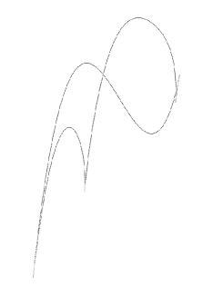
Figure 2. The polar curve of the quartic surface projected on a plane.

The first factor of degree $10$ has $4$ real roots corresponding to the smooth points of the surface with a tangent plane orthogonal to the $x$-direction. The second factor of multiplicity $2$ corresponds to points of the polar variety which project in the $(x,y)$-plane onto the same point. Geometrically speaking, we have a double folding of the surface in the $z$-direction above these values. There are two such real points in our example. The last factor of multiplicity $3$ corresponds to cusp points on the discriminant curve, which are the projection of a “fronce” or a pleat of the surface. There are $4$ such real points. Notice that the branches of the discriminant curve between two of these cusp points and one of the double folding points form a very tiny loop, which is difficult to observe at this scale.

These phenomena can be explained from an algebraic point of view, as we will see hereafter. They have also been analyzed from a singularity theory point of view. A well-know result in singularity theory, due to H. Whitney (see [31, 25, 2]) asserts that the singularities of the projection of a generic surface onto a plane are of $3$ types:

• a regular point on the contour curve corresponding to a fold of the surface,

• a cusp corresponding to a pleat,

• a double point corresponding to the projection of two transversal folds.

These are stable singularities, which remain by a small perturbation of the surface or of the direction of projection. For a more complete analysis of the singularities of the apparent contour, see also [29].

We are now going to analyze the algebraic side of these geometric properties for generic polynomials of a given degree. Suppose given a positive integer $d\geq 3$ and a homogeneous polynomial

$$\begin{array}[]{ll}P(X_{1},X_{2},X_{3}):=\sum_{0\leq i,j;i+j\leq d}&U_{i,j}X_{1}^{i}X_{2}^{j}X_{3}^{d-i-j}\in{\mathbb{U}}[X_{1},X_{2},X_{3}],\end{array}$$

where ${\mathbb{U}}$ is the universal coefficients ring $\mathbbm{Z}[U_{i,j}]$. In this section we will study the discriminant of the discriminant of $P$. Here is the first factorization we can get as a specialization of the iterated resultant we studied in the previous section.

Proposition 6.1.

We have the equality in ${\mathbb{U}}$:

$$U_{0,0}^{2\,d^{2}-2d-1}{\mathrm{Disc}}_{X_{2}}({\mathrm{Disc}}_{X_{3}}(P(1,X_{2},X_{3})))={\mathrm{Disc}}_{X_{1}:X_{2}:X_{3}}(P)\times\\ {\operatorname{Res}}_{X_{1}:X_{2}:X_{3}}(P,\partial_{3}P,\partial_{3}^{2}P)\times{\operatorname{Res}}_{X_{1}:\cdots:X_{4}}(P,\delta_{3,4}P,\partial_{3}P,\delta_{3,4}\partial_{3}P).$$

The iterated discriminant ${\mathrm{Disc}}_{X_{2}}({\mathrm{Disc}}_{X_{3}}(P(1,X_{2},X_{3})))$ is homogeneous with respect to the set of coefficients $U_{i,j}$ of degree $4\,(d-1)\,(d^{2}-d-1)$.

Proof.

This is essentially a specialization of the formula given in Proposition 5.6, which yields in our case the equality

$${\mathrm{Disc}}_{X_{2}}({\operatorname{Res}}_{X_{3}}(P(1,X_{2},X_{3}),\partial_{3}P(1,X_{2},X_{3})))={\mathrm{Disc}}(P,\partial_{3}P)\times\\ {\operatorname{Res}}(P,\delta_{3,4}P,\partial_{3}P,\delta_{3,4}\partial_{3}P).$$

On the one hand, we know by definition of the discriminant and properties of resultants, that

$${\operatorname{Res}}(P,\partial_{3}P,X_{1}){\mathrm{Disc}}(P,\partial_{3}P)$$

$$= {\operatorname{Res}}(P,\partial_{3}P,\partial_{2}P\partial_{3}^{2}P-\partial_{3}P\partial_{2}\partial_{3}P)$$

$$= {\operatorname{Res}}(P,\partial_{3}P,\partial_{2}P\partial_{3}^{2}P)$$

(6.2) $$= {\operatorname{Res}}(P,\partial_{3}P,\partial_{2}P)\times{\operatorname{Res}}(P,\partial_{3}P,\partial_{3}^{2}P).$$

Moreover, by Euler identity we have $dP=X_{1}\partial_{1}P+X_{2}\partial_{2}P+X_{3}\partial_{3}P$ from we deduce that

$${d^{d-1}{\operatorname{Res}}(P,\partial_{3}P,X_{1})} = {\operatorname{Res}}(X_{2}\partial_{2}P,\partial_{3}P,X_{1})$$

$$= {\operatorname{Res}}(X_{2},\partial_{3}P,X_{1})\times{\operatorname{Res}}(\partial_{2}P,\partial_{3}P,X_{1})$$

$$= d\,U_{0,0}{\operatorname{Res}}(\partial_{2}P,\partial_{3}P,X_{1}).$$

Again by Euler identity, the relation (2.4) yields

$${d^{(d-1)^{2}}{\operatorname{Res}}(P,\partial_{3}P,\partial_{2}P)} = {\operatorname{Res}}(X_{1}\partial_{1}P,\partial_{3}P,\partial_{2}P)$$

$$= {\operatorname{Res}}(X_{1},\partial_{3}P,\partial_{2}P){\operatorname{Res}}(\partial_{1}P,\partial_{3}P,\partial_{2}P)$$

$$= d^{d^{2}-3d+3}{\operatorname{Res}}(\partial_{2}P,\partial_{3}P,X_{1}){\mathrm{Disc}}(P)$$

and by substitution in (6.2) and simplification by ${\operatorname{Res}}(\partial_{2}P,\partial_{3}P,X_{1})$ and $d^{d-2}$, we get that

$$U_{0,0}{\mathrm{Disc}}(P,\partial_{3}P)={\mathrm{Disc}}(P){\operatorname{Res}}(P,\partial_{3}P,\partial_{3}^{2}P)$$

so that

$$U_{0,0}{\mathrm{Disc}}_{X_{2}}({\operatorname{Res}}_{X_{3}}(P(1,X_{2},X_{3}),\partial_{3}P(1,X_{2},X_{3})))={\mathrm{Disc}}(P)\times\\ {\operatorname{Res}}(P,\partial_{3}P,\partial_{3}^{2}P)\times{\operatorname{Res}}_{X_{1}:\cdots:X_{4}}(P(X_{3}),\delta_{X_{3},X_{4}}(P),\partial_{3}P(X_{3}),\delta_{X_{3},X_{4}}(\partial_{3}P)).$$

On the other hand,

$${\mathrm{Disc}}_{X_{2}}({\operatorname{Res}}_{X_{3}}(P(1,X_{2},X_{3}),\partial_{3}P(1,X_{2},X_{3})))$$

$$= {\mathrm{Disc}}_{X_{2}}(U_{0,0}{\mathrm{Disc}}_{X_{3}}(P(1,X_{2},X_{3})))$$

$$= U_{0,0}^{2\,(d(d-1)-1)}{\mathrm{Disc}}_{X_{2}}({\mathrm{Disc}}_{X_{3}}(P(1,X_{2},X_{3})))$$

$$= U_{0,0}^{2d^{2}-2d-2}{\mathrm{Disc}}_{X_{2}}({\mathrm{Disc}}_{X_{3}}(P(1,X_{2},X_{3})))$$

since ${\mathrm{Disc}}_{X_{3}}(P(1,X_{2},X_{3}))$ is of degree $d(d-1)$ in $X_{2}$ and the discriminant of a polynomial of degree $D$ is homogeneous of degree $2\,(D-1)$ in its coefficients. The claimed formula then follows immediately.

Concerning the degree, observe that ${\mathrm{Disc}}_{X_{3}}(P(1,X_{2},X_{3}))$ has coefficients of degree $2\,(d-1)$ in the coefficients of $P$. The discriminant of a polynomial of degree $D$ being homogeneous of degree $2\,(D-1)$ in its coefficients, we obtain that ${\mathrm{Disc}}_{X_{2}}({\mathrm{Disc}}_{X_{3}}(P(1,X_{2},X_{3})))$ is of degree

$$2(d(d-1)-1)\times 2\,(d-1)=4(d-1)(d^{2}-d-1)$$

since the degree of ${\mathrm{Disc}}_{X_{3}}(P(1,X_{2},X_{3})))$ in $X_{2}$ is $D=d(d-1)$. ∎

In the factorization of ${\mathrm{Disc}}_{X_{2}}({\mathrm{Disc}}_{X_{3}}(P))$ given in this proposition, we only know that the factor ${\mathrm{Disc}}(P)$ is known to be irreducible in ${\mathbb{U}}$. The remaining of this section is devoted to the study of the full factorization of the two other factors. We begin with the study of the factor appearing in Proposition 6.1 which corresponds to the resultant of $P$, its first and second derivatives with respect to $X_{3}$.

Lemma 6.2.

Let $\SS$ be a commutative ring and suppose given a linear form $L=a\,X_{1}+b\,X_{2}+c\,X_{3}\in\SS[X_{1},X_{2},X_{3}]$ and a homogeneous polynomial $Q\in\SS[X_{1},X_{2},X_{3}]$ of degree $d-1\geq 2$. Then

$${\operatorname{Res}}(LQ,\partial_{3}(LQ),\partial_{3}^{2}(LQ))=2^{2(d-1)}c^{3\,d-4}{\operatorname{Res}}(L,Q,\partial_{3}(Q))^{3}\times{\operatorname{Res}}(Q,\partial_{3}(Q),\partial_{3}^{2}(Q)).$$

Proof.

It is a straightforward computation using the properties of the resultants:

$${\operatorname{Res}}(LQ,\partial_{3}(LQ),\partial_{3}^{2}(LQ)) = {\operatorname{Res}}(LQ,cQ+L\partial_{3}(Q),2c\partial_{3}(Q)+L\,\partial_{3}^{2}(Q))$$

$$= {\operatorname{Res}}(L,c\,Q,2c\,\partial_{3}(Q))\times$$

$${\operatorname{Res}}(Q,L\,\partial_{3}(Q),2\,c\,\partial_{3}(Q)+L\,\partial_{3}^{2}(Q))$$

$$= 2^{d-1}c^{2d-3}{\operatorname{Res}}(L,Q,\partial_{3}(Q)){\operatorname{Res}}(Q,L,2\,c\,\partial_{3}(Q))\times$$

$${\operatorname{Res}}(Q,\partial_{3}(Q),L\,\partial_{3}^{2}(Q))$$

$$= 2^{2(d-1)}c^{2d-3+d-1}{\operatorname{Res}}(L,Q,\partial_{3}Q)^{2}\times$$

$${\operatorname{Res}}(Q,\partial_{3}(Q),L){\operatorname{Res}}(Q,\partial_{3}(Q),\partial_{3}^{2}(Q))$$

$$= 2^{2(d-1)}c^{3d-4}{\operatorname{Res}}(L,Q,\partial_{3}(Q))^{3}\times$$

$${\operatorname{Res}}(Q,\partial_{3}(Q),\partial_{3}^{2}(Q)).$$

∎

Proposition 6.3.

The following equality holds in ${\mathbb{U}}$:

$${\operatorname{Res}}_{X_{1}:X_{2}:X_{3}}(P,\partial_{3}P,\partial_{3}^{2}P)=2^{d(d-1)}U_{0,0}^{2}\,{\mathfrak{F}}(P)$$

where ${\mathfrak{F}}(P)$ is an irreducible homogeneous polynomial in ${\mathbb{U}}$ of degree $3d(d-2)$.

Proof.

We rewrite $P$ as

$$P=U_{0,0}X_{3}^{d}+c_{1}X_{3}^{d-1}+\cdots+c_{d-2}X_{3}^{2}+c_{d-1}X_{3}+c_{d}$$

where the $c_{i}$’s are homogeneous polynomials in ${\mathbb{U}}[X_{1},X_{2}]$ of degree $i$ respectively;  we have

$$\partial_{3}P = \operatorname{dA}_{0,0}X_{3}^{d-1}+(d-1)c_{1}X_{3}^{d-2}+\cdots+2c_{d-2}X_{3}+c_{d-1,}$$

$$\partial_{3}^{2}P = d(d-1)U_{0,0}X_{3}^{d-2}+(d-1)(d-2)c_{1}X_{3}^{d-3}+\cdots+2c_{d-2}.$$

Consider the incidence variety

$$\mathcal{W}:=\{(x_{1}:x_{2}:x_{3})\times(a_{i,j})\in\mathbbm{P^{\mathrm{2}}}\times\mathbbm{A}^{\mathrm{d(d+1)/2}}\operatorname{such}\operatorname{that}P=\partial_{3}P=\partial_{3}^{2}P=0\}$$

whose canonical projection onto the second factor, i.e. by $\pi_{2}:\mathcal{W}\rightarrow\mathbbm{A}^{\mathrm{d(d+1)/2}}$, is the variety of pure codimension one defined by the equation ${\operatorname{Res}}(P,\partial_{3}P,\partial_{3}^{2}P)=0$. Considering the canonical projection onto its first factor $\pi_{1}:\mathcal{W}\rightarrow\mathbbm{P}^{2}$, which is surjective, we observe that $\pi_{1}^{-1}(0:0:1)$ is the hyperplane $\{U_{0,0}=0\}$ in $\mathbbm{A^{\mathrm{d(d+1)/2}}}$ and that $\pi_{1}^{-1}(x_{1}:x_{2}:x_{3})$ is a linear space of codimension 3 in $\mathbbm{A^{\mathrm{d(d+1)/2}}}$ if $(x_{1}:x_{2}:x_{3})\neq(0:0:1)\in\mathbbm{P}^{2}$ (just observe that in this case the three conditions $c_{d}=0,c_{d-1}=0,c_{d-2}=0$ are non trivial and that $\partial_{3}P$ does not depend on $c_{d}$ and that $\partial_{3}^{2}P$ does not depend on $c_{d}$ and $c_{d-1}$). It follows that $\mathcal{W}=\mathcal{W}_{0}\cup\mathcal{W}_{3}$ where $\mathcal{W}_{0}$ is the irreducible variety defined by $\{U_{0,0}=0\}$ and $\mathcal{W}_{3}$, which is the closure of the fiber bundle $\pi_{1}^{-1}(\mathbbm{P}^{2}\setminus(0:0:1))\rightarrow\mathbbm{P}^{2}\setminus(0:0:1)$ in $\mathbbm{P^{\mathrm{2}}}\times\mathbbm{A^{\mathrm{d(d+1)/2}}}$, is an irreducible variety of codimension 3. We deduce that $\pi_{2}(\mathcal{W})$ is the union of two irreducible varieties: $\pi_{2}(\mathcal{W}_{0})$ whose defining equation is $\{U_{0,0}=0\}$ and $\pi_{2}(\mathcal{W}_{3})$. Therefore, we obtain that, in ${\mathbb{U}}$,

$${\operatorname{Res}}(P,\partial_{3}P,\partial_{3}^{2}P)=c(d)U_{0,0}^{a(d)}R_{d}^{r(d)}$$

where $c(d),a(d),r(d)$ are all positive integers (in particular, they are nonzero) which may only depend on $d$, the degree of $P$, and $R_{d}$ is an irreducible polynomial in ${\mathbb{U}}$. In order to determine $c(d),a(d),r(d)$ we will use a particular specialization and some properties of the resultants.

First, it is easy to check by hand (or with a computer), that the case $d=3$ gives, in ${\mathbb{U}}$,

$${\operatorname{Res}}(P,\partial_{3}P,\partial_{3}^{2}P)=2^{6}U_{0,0}^{2}{\mathfrak{F}}(P)$$

where ${\mathfrak{F}}(P)$ is an irreducible polynomial. Moreover, if $\phi$ denotes the homogeneous specialization which sends all the coefficients of $c_{d}$ to 0, we have $\phi(P)=X_{3}\,Q$, where $Q$ is a generic homogeneous polynomial of degree $d-1$. By Lemma 6.2, we get

$$\phi({\operatorname{Res}}(P,\partial_{3}P,\partial_{3}^{2}P))=2^{2(d-1)}{\operatorname{Res}}(Q,\partial_{3}Q,X_{3})^{3}{\operatorname{Res}}(Q,\partial_{3}Q,\partial_{3}^{2}Q).$$

So, if we proceed by induction on the integer $d$, we obtain

$$\phi({\operatorname{Res}}(P,\partial_{3}P,\partial_{3}^{2}P)) = 2^{2(d-1)}{\operatorname{Res}}(Q,\partial_{3}Q,X_{3})^{3}\times 2^{(d-1)(d-2)}U_{0,0}^{a(d-1)}{\mathfrak{F}}(Q)$$

$$= 2^{d(d-1)}U_{0,0}^{2}{\operatorname{Res}}(Q,\partial_{3}Q,X_{3})^{3}{\mathfrak{F}}(Q)$$

where we notice that ${\operatorname{Res}}(Q,\partial_{3}Q,X_{3})={\operatorname{Res}}(c_{d-1},c_{d-2})$ is an irreducible polynomial in ${\mathbb{U}}$ (it is the resultant of two generic homogeneous polynomials) which does not depend on $U_{0,0}$. Since we must also have

$$\phi({\operatorname{Res}}(P,\partial_{3}P,\partial_{3}^{2}P))=c(d)U_{0,0}^{a(d)}\phi({\mathfrak{F}}(P))^{r(d)}$$

we deduce by comparison that, for all $d\geq 3$,

• $c(d)$ divides $2^{d(d-1)}$,

• $r(d)=1$ (since the specialization of $R_{d}$ by $\phi$ produces an irreducible and reduced factor),

• $a(d)\leq 2$.

It is easy to see that 2 divides $\partial_{3}^{2}P$ and hence that $2^{d(d-1)}$ divides ${\operatorname{Res}}(P,\partial_{3}P,\partial_{3}^{2}P)$. This implies that $2^{d(d-1)}$ divides $c(d)$ and hence, since we already noted that $c(d)$ divides $2^{d(d-1)}$, $c(d)=2^{d(d-1)}$. To conclude the proof, it remains to show that $a(d)\geq 2$ for all $d\geq 3$, that is to say that $U_{0,0}^{2}$ divides ${\operatorname{Res}}(P,\partial_{3}P,\partial_{3}^{2}P)$ in ${\mathbb{U}}$. Moreover, it is sufficient to show that $U_{0,0}^{2}$ divides

$$\mathfrak{R}:={\operatorname{Res}}(d(d-1)P,(d-1)\partial_{3}P,\partial_{3}^{2}P)$$

since

$${\operatorname{Res}}(d(d-1)P,(d-1)\partial_{3}P,\partial_{3}^{2}P)=d(d-1)^{(d-1)(d-2)}\times(d-1)^{d(d-2)}\times{\operatorname{Res}}(P,\partial_{3}P,\partial_{3}^{2}P).$$

Using Euler identity several times, we get

$$\mathfrak{R} = {\operatorname{Res}}((d-1)X_{1}\partial_{1}P+(d-1)X_{2}\partial_{2}P,(d-1)\partial_{3}P,\partial_{3}^{2}P)$$

$$= {\operatorname{Res}}(X_{1}^{2}\partial_{1}^{2}P+2X_{1}X_{2}\partial_{1}\partial_{2}P+X_{2}^{2}\partial_{2}^{2}P,X_{1}\partial_{1}\partial_{3}P+X_{2}\partial_{2}\partial_{3}P,\partial_{3}^{2}P).$$

It is clear that $\partial_{3}^{2}P\in(X_{1},X_{2},U_{0,0}X_{3})$ and that

$$X_{1}\partial_{1}\partial_{3}P+X_{2}\partial_{2}\partial_{3}P\in(X_{1},X_{2})\subset(X_{1},X_{2},U_{0,0}X_{3}).$$

Moreover, $X_{1}^{2}\partial_{1}^{2}P+2X_{1}X_{2}\partial_{1}\partial_{2}P+X_{2}^{2}\partial_{2}^{2}P\in(X_{1},X_{2})^{2}\subset(X_{1},X_{2},U_{0,0}X_{3})^{2}$. Therefore, the divisibility property of resultants implies that

$${\operatorname{Res}}(X_{1},X_{2},U_{0,0}X_{3})^{2\times 1\times 1}\operatorname{divides}\mathfrak{R},$$

and since ${\operatorname{Res}}(X_{1},X_{2},U_{0,0}X_{3})=U_{0,0}$, we are done.

Finally, the degree of ${\mathfrak{F}}(P)$ in the coefficients of $P$ is given by the formula

$$d\,(d-1)+d\,(d-2)+(d-1)\,(d-2)-2=3\,d\,(d-2).$$

∎

We now turn to the study of the third factor appearing in the factorization of ${\mathrm{Disc}}_{X_{2}}({\mathrm{Disc}}_{X_{3}}(P))$ in Proposition 6.1.

Proposition 6.4.

Assuming that $d\geq 4$, we have the following equality between homogeneous polynomials in ${\mathbb{U}}$ of degree $2(d-1)(2d^{2}-4d+1)$:

$$2^{d(d-1)}{\operatorname{Res}}_{X_{1}:\cdots:X_{4}}(P,\delta_{3,4}P,\partial_{3}P,(\delta_{3,4}\partial_{3})P)=\\ {\operatorname{Res}}_{X_{1}:X_{2}:X_{3}}(P,\partial_{3}P,\partial_{3}^{2}P)^{2}\times{\operatorname{Res}}_{X_{1}:\cdots:X_{4}}(P,\partial_{3}P,\delta_{3,4}^{2}P,(\delta_{3,4}^{2}\partial_{3}-2\delta_{3,4}^{3})P).$$

Proof.

Using known properties of resultants and equalities (2.6) and (2.7), we get the equalities

$${\operatorname{Res}}(P,\delta_{3,4}P,\partial_{3}P,\delta_{3,4}\partial_{3}P) = {\operatorname{Res}}(P,\partial_{3}P+(X_{4}-X_{3})\delta_{3,4}^{2}P,\partial_{3}P,\delta_{3,4}\partial_{3}P)$$

$$= {\operatorname{Res}}(P,(X_{4}-X_{3})\delta_{3,4}^{2}P,\partial_{3}P,\delta_{3,4}\partial_{3}P)$$

$$= {\operatorname{Res}}(P,(X_{4}-X_{3}),\partial_{3}P,\delta_{3,4}\partial_{3}P)\times$$

$${\operatorname{Res}}(P,\delta_{3,4}^{2}P,\partial_{3}P,\partial_{3}^{2}P+(X_{4}-X_{3})\delta_{3,4}^{2}\partial_{3}P)$$

$$= {\operatorname{Res}}(P,\partial_{3}P,\partial^{2}_{3}P)\times$$

$${\operatorname{Res}}(P,\delta_{3,4}^{2}P,\partial_{3}P,\partial_{3}^{2}P+(X_{4}-X_{3})\delta_{3,4}^{2}\partial_{3}P).$$

Let us denote

$$\mathcal{S}(P):={\operatorname{Res}}(P,\delta_{3,4}^{2}P,\partial_{3}P,\partial_{3}^{2}P+(X_{4}-X_{3})\delta_{3,4}^{2}\partial_{3}P).$$

Since $\partial_{3}^{2}P=2\delta_{3,4}^{2}P-2(X_{4}-X_{3})\delta_{3,4}^{3}P$ in ${\mathbb{U}}$, we deduce that, in ${\mathbb{U}}$,

$$2^{d(d-1)(d-2)}\mathcal{S}(P) = {\operatorname{Res}}(P,2\delta_{3,4}^{2}P,\partial_{3}P,\partial_{3}^{2}P+(X_{4}-X_{3})\delta_{3,4}^{2}\partial_{3}P)$$

$$= {\operatorname{Res}}(P,2\delta_{3,4}^{2}P,\partial_{3}P,(X_{4}-X_{3})(\delta_{3,4}^{2}\partial_{3}-2\delta_{3,4}^{3})P)$$

$$= {\operatorname{Res}}(P,2\delta_{3,4}^{2}P,\partial_{3}P,(X_{4}-X_{3}))\times$$

$${\operatorname{Res}}(P,2\delta_{3,4}^{2}P,\partial_{3}P,(\delta_{3,4}^{2}\partial_{3}-2\delta_{3,4}^{3})P)$$

$$= {\operatorname{Res}}(P,\partial_{3}^{2}P,\partial_{3}P,(X_{4}-X_{3}))\times$$

$${\operatorname{Res}}(P,2\delta_{3,4}^{2}P,\partial_{3}P,(\delta_{3,4}^{2}\partial_{3}-2\delta_{3,4}^{3})P)$$

$$= 2^{d(d-1)(d-3)}{\operatorname{Res}}(P,\partial_{3}^{2}P,\partial_{3}P)\times$$

$${\operatorname{Res}}(P,\delta_{3,4}^{2}P,\partial_{3}P,(\delta_{3,4}^{2}\partial_{3}-2\delta_{3,4}^{3})P).$$

Therefore, we have

$$2^{d(d-1)}{\operatorname{Res}}(P,\delta_{3,4}P,\partial_{3}P,(\delta_{3,4}\partial_{3})P)={\operatorname{Res}}(P,\partial_{3}P,\partial_{3}^{2}P)^{2}\times\\ {\operatorname{Res}}((P,\partial_{3}P,\delta_{3,4}^{2}P,(\delta_{3,4}^{2}\partial_{3}-2\delta_{3,4}^{3})P).$$

The claimed formula for the degree of ${\operatorname{Res}}(P,\delta_{3,4}P,\partial_{3}P,(\delta_{3,4}\partial_{3})P)$ follows immediately by specialization of the formula given in Lemma 5.4. ∎

As a consequence, to get the full factorization of ${\mathrm{Disc}}_{X_{2}}({\mathrm{Disc}}_{X_{3}}(P))$ it only remains to study the factorization of the term

$${\mathcal{R}}(P):={\operatorname{Res}}_{X_{1}:\cdots:X_{4}}(P,\partial_{3}P,\delta_{3,4}^{2}P,(\delta_{3,4}^{2}\partial_{3}-2\delta_{3,4}^{3})P)$$

whose degree in the coefficients of $P$ is

$$2\,(d-1)\,(2d^{2}-4d+1)-2(d\,(d-1)+d\,(d-2)+(d-1)\,(d-2))=2\,(2d-3)\,(d^{2}-3d+1).$$

This is the aim of the next proposition. We begin with two technical lemmas.

Lemma 6.5.

Let $\SS$ be a commutative ring and suppose given a linear form $L=a\,X_{1}+b\,X_{2}+c\,X_{3}\in\SS[X_{1},X_{2},X_{3}]$ and a homogeneous polynomial $Q\in\SS[X_{1},X_{2},X_{3}]$ of degree $d-1\geq 2$. Then

$${\operatorname{Res}}_{X_{1}:\cdots:X_{4}}(LQ,\partial_{3}(LQ),\delta_{3,4}(LQ),\delta_{3,4}\partial_{3}(LQ))=2^{2(d-1)}c^{2(d-1)(3d-5)}\times\\ {\operatorname{Res}}_{X_{1}:X_{2}:X_{3}}(L,Q,\partial_{3}Q)^{6}\times{\operatorname{Res}}_{X_{1}:\cdots:X_{4}}(L(X_{4}),Q,\partial_{3}Q,\delta_{3,4}^{2}Q)^{4}\times\\ {\operatorname{Res}}_{X_{1}:\cdots:X_{4}}(Q,\delta_{3,4}Q,\partial_{3}Q,\delta_{3,4}\partial_{3}Q).$$

Proof.

Set $P:=LQ$. Applying (LABEL:eq:dr1) with $P_{2}=\partial_{3}(P)$ and

$$\partial_{3}P(X_{4})=\partial_{3}P(X_{3})+(X_{4}-X_{3})\,\delta_{3,4}\partial_{3}P,$$

we obtain the decomposition

$${\operatorname{Res}}(P,\partial_{3}(P),\delta_{3,4}(P),\delta_{3,4}\partial_{3}(P))$$

$$= c^{(d-1)(d-2)}\,\times{\operatorname{Res}}(L(X_{4}),Q(X_{3}),\partial_{3}(P),\delta_{3,4}\partial_{3}(P))^{2}\times$$

$${\operatorname{Res}}(Q,\delta_{3,4}(Q),\partial_{3}(P),\delta_{3,4}\partial_{3}(P))$$

$$= c^{(d-1)(d-2)}\,R_{1}^{2}\,R_{2}.$$

Using the relations

$$\partial_{3}(P) = \partial_{3}(L)\,Q+L\,\partial_{3}(Q),$$

$$\delta_{3,4}\partial_{3}(P) = \partial_{3}(L)\,\delta_{3,4}(Q)+\delta_{3,4}(L)\,\partial_{3}(Q)+L(X_{4})\delta_{3,4}\partial_{3}(Q),$$

we can decompose further the previous expressions:

$$R_{1}:=\hbox to0.0pt{$\displaystyle{\operatorname{Res}}(L(X_{4}),Q,\partial_{3}(P),\delta_{3,4}\partial_{3}(P))$\hss}$$

$$= {\operatorname{Res}}(L(X_{4}),Q,L\,\partial_{3}(Q),\partial_{3}(L)\,\delta_{3,4}(Q)+\delta_{3,4}(L)\,\partial_{3}(Q))$$

$$= {\operatorname{Res}}(L(X_{4}),Q,L,c\,\delta_{3,4}(Q)+c\,\partial_{3}(Q))\times{\operatorname{Res}}(L(X_{4}),Q,\partial_{3}(Q),c\,\delta_{3,4}(Q))$$

$$= {\operatorname{Res}}(L(X_{4}),Q,c\,(X_{3}-X_{4}),c\,(\delta_{3,4}(Q)+\partial_{3}(Q)))\times$$

$$c^{(d-1)(d-2)}{\operatorname{Res}}(L(X_{4}),Q,\partial_{3}(Q),\delta_{3,4}(Q))$$

$$= c^{(d-1)+(d-1)(d-2)}{\operatorname{Res}}(L,Q,2\partial_{3}(Q))\times$$

$$c^{(d-1)(d-2)}{\operatorname{Res}}(L(X_{4}),Q,\partial_{3}(Q),\delta_{3,4}(Q))$$

$$= 2^{d-1}c^{(d-1)(2d-3)}{\operatorname{Res}}(L,Q,\partial_{3}(Q))\times{\operatorname{Res}}(L(X_{4}),Q,\partial_{3}(Q),\delta_{3,4}(Q)).$$

Now, using the relation $\delta_{3,4}(Q)=\partial_{3}(Q)+(X_{4}-X_{3})\delta_{3,4}^{2}(Q)$, we have

$${\operatorname{Res}}(Q,\partial_{3}(Q),\delta_{3,4}(Q),L(X_{4}))$$

$$= {\operatorname{Res}}(Q,\partial_{3}(Q),(X_{4}-X_{3})\,\delta_{3,4}^{2}(Q),L(X_{4}))$$

$$= {\operatorname{Res}}(L,Q,\partial_{3}(Q))\times{\operatorname{Res}}(Q,\partial_{3}(Q),\delta_{3,4}^{2}(Q),L(X_{4})).$$

We deduce that

$$R_{1}=2^{d-1}c^{(d-1)(2d-3)}{\operatorname{Res}}(L,Q,\partial_{3}(Q))^{2}\times{\operatorname{Res}}(Q,\partial_{3}(Q),\delta_{3,4}^{2}(Q),L(X_{4})).$$

Similarly, we have

$$R_{2}=\hbox to0.0pt{$\displaystyle{\operatorname{Res}}(Q,\delta_{3,4}(Q),\partial_{3}(P),\delta_{3,4}\partial_{3}(P))$\hss}$$

$$= {\operatorname{Res}}(Q,\delta_{3,4}(Q),L\,\partial_{3}(Q),\delta_{3,4}(L)\partial_{3}(Q)+L(X_{4})\,\delta_{3,4}\partial_{3}(Q))$$

$$= {\operatorname{Res}}(Q,\delta_{3,4}(Q),L,\delta_{3,4}(L)\partial_{3}(Q)+L(X_{4})\,\delta_{3,4}\partial_{3}(Q))\times$$

$${\operatorname{Res}}(Q,\delta_{3,4}(Q),\partial_{3}(Q),L(X_{4})\,\delta_{3,4}\partial_{3}(Q))$$

$$= {\operatorname{Res}}(Q,\delta_{3,4}(Q),L,c\,\partial_{3}(Q)(X_{4}))\times{\operatorname{Res}}(Q,\delta_{3,4}(Q),\partial_{3}(Q),L(X_{4}))$$

$$\times{\operatorname{Res}}(Q,\delta_{3,4}(Q),\partial_{3}(Q),\delta_{3,4}\partial_{3}(Q))$$

$$= c^{(d-1)(d-2)}{\operatorname{Res}}(Q,\partial_{3}(Q),\delta_{3,4}(Q),L(X_{4}))^{2}\times$$

$${\operatorname{Res}}(Q,\delta_{3,4}(Q),\partial_{3}(Q),\delta_{3,4}\partial_{3}(Q)),$$

since

$$c\partial_{3}(Q)+L(X_{4})\delta_{3,4}\partial_{3}Q-L(X_{3})\,\delta_{3,4}\partial_{3}(Q)=c\partial_{3}(Q)(X_{4}),$$

and

$${\operatorname{Res}}(Q,\delta_{3,4}(Q),L,\partial_{3}(Q)(X_{4}))={\operatorname{Res}}(Q,\partial_{3}(Q),\delta_{3,4}(Q),L(X_{4})).$$

using the relation (6), we deduce that

$$R_{2}=c^{(d-1)\,(d-2)}{\operatorname{Res}}(L,Q,\partial_{3}Q)^{2}\times{\operatorname{Res}}(L(X_{4}),Q,\partial_{3}Q,\delta_{3,4}^{2}Q)^{2}\times\\ {\operatorname{Res}}(Q,\delta_{3,4}(Q),\partial_{3}(Q),\delta_{3,4}\partial_{3}(Q)).$$

By (6), squaring $R_{1}$ and taking the product with $R_{2}$ and $c^{(d-1)(d-2)}$, we obtain the expected decomposition. ∎

Lemma 6.6.

Let $\SS$ be a commutative ring and suppose given a linear form $L=a\,X_{1}+b\,X_{2}+c\,X_{3}\in\SS[X_{1},X_{2},X_{3}]$ and a homogeneous polynomial $Q\in\SS[X_{1},X_{2},X_{3}]$ of degree $d-1\geq 2$. Then

$${\mathcal{R}}(LQ)=c^{6d^{2}-22d+18}\,{\operatorname{Res}}(L(X_{4}),Q,\partial_{3}(Q),\delta_{3,4}^{2}(Q))^{4}\,{\mathcal{R}}(Q).$$

Proof.

Set $P:=LQ$. By Proposition 6.4 and Lemma 6.2, we have

$$2^{d(d-1)}{\operatorname{Res}}(P,\delta_{3,4}(P),\partial_{3}(P),\delta_{3,4}\partial_{3}(P))$$

$$= {\operatorname{Res}}(P,\partial_{3}(P),\partial_{3}^{2}(P))^{2}\,{\mathcal{R}}(P)$$

$$= \left(2^{2(d-1)}c^{3d-4}{\operatorname{Res}}(L,Q,\partial_{3}(Q))^{3}\,{\operatorname{Res}}(Q,\partial_{3}(Q),\partial_{3}^{2}(Q))\right)^{2}{\mathcal{R}}(P)$$

$$= 2^{4(d-1)}c^{6d-8}{\operatorname{Res}}(L,Q,\partial_{3}(Q))^{6}\,{\operatorname{Res}}(Q,\partial_{3}(Q),\partial_{3}^{2}(Q))^{2}\,{\mathcal{R}}(P).$$

Moreover, by Lemma 6.5 and Proposition 6.4 we also have

$${\operatorname{Res}}(P,\delta_{3,4}(P),\partial_{3}(P),\delta_{3,4}\partial_{3}(P))$$

$$= 2^{2(d-1)}c^{2(d-1)(3d-5)}{\operatorname{Res}}(L,Q,\partial_{3}Q)^{6}\,{\operatorname{Res}}(L(X_{4}),Q,\partial_{3}(Q),\delta_{3,4}^{2}(Q))^{4}\times$$

$${\operatorname{Res}}(Q,\delta_{3,4}Q,\partial_{3}Q,\delta_{3,4}\partial_{3}Q)$$

$$= 2^{-d(d-1)}c^{2(d-1)(3d-5)}{\operatorname{Res}}(L,Q,\partial_{3}Q)^{6}\,{\operatorname{Res}}(L(X_{4}),Q,\partial_{3}(Q),\delta_{3,4}^{2}(Q))^{4}\times$$

$${\operatorname{Res}}(Q,\partial_{3}Q,\partial_{3}^{2}Q)^{2}{\mathcal{R}}(Q)$$

and the claimed formula follows by comparison. ∎

Proposition 6.7.

Assuming that $d\geq 4$, we have

$$\mathcal{R}(P)=U_{0,0}^{2d(d-1)-6}{\mathfrak{U}}(P)^{2},$$

where ${\mathfrak{U}}(P)$ is irreducible in ${\mathbb{U}}$ of degree $2\,d\,(d-2)\,(d-3)$.

Proof.

We first prove that $U_{0,0}^{2d(d-1)-6}$ divides ${\mathcal{R}}(P)$ in ${\mathbb{U}}$. Gathering the results of the propositions 6.1, 6.3, 6.4 and 6.7 we obtain the following equality in ${\mathbb{U}}$:

(6.5) $$U_{0,0}^{2d(d-1)-6}{\mathrm{Disc}}_{X_{2}}({\mathrm{Disc}}_{X_{3}}(P(1,X_{2},X_{3})))=U_{0,0}{\mathrm{Disc}}_{X_{1}:X_{2}:X_{3}}(P){\mathfrak{F}}(P)^{3}{\mathcal{R}}(P).$$

In order to prove that $U_{0,0}^{2d(d-1)-6}$ divides ${\mathcal{R}}(P)$, it is thus sufficient to prove that $U_{0,0}$ divides ${\mathrm{Disc}}_{X_{2}}({\mathrm{Disc}}_{X_{3}}(P(1,X_{2},X_{3})))$. Rewrite the polynomial $P$ as

$$P:=U_{0,0}X_{3}^{d}+a_{d-1}X_{3}^{d-1}+\cdots+a_{1}X_{3}+a_{0}$$

where the $a_{i}$’s are homogeneous polynomials in $X_{1},X_{2}$. If one specializes $U_{0,0}$ to 0 then $P$ specializes to a polynomial of degree $d-1$ in $X_{3}$ and hence, by a well-known property of discriminants we have

$${\mathrm{Disc}}_{X_{3}}(P(1,X_{2},X_{3}))=(-1)^{d}a_{d-1}(1,X_{2})^{2}{\mathrm{Disc}}^{\prime}_{X_{3}}(P(1,X_{2},X_{3}))$$

where ${\mathrm{Disc}}^{\prime}_{X_{3}}(P(1,X_{2},X_{3}))$ denotes the discriminant of $P$ as a polynomial of degree $d-1$ (and not $d$). But then, the discriminant with respect to $X_{2}$ of the above quantity equals 0 since it contains a square factor. This implies that $U_{0,0}$ divides ${\mathrm{Disc}}_{X_{2}}({\mathrm{Disc}}_{X_{3}}(P(1,X_{2},X_{3})))$.

Observe now that by Proposition 5.4 and Proposition 6.4, ${\mathcal{R}}(P)$ is a square and hence can be decomposed as

$${\mathcal{R}}(P)=c(d)^{2}U_{0,0}^{2d(d-1)-6}\,{\mathfrak{R}}_{1}^{2\,r_{1}(d)}(P)\,{\mathfrak{R}}_{2}^{2\,r_{2}(d)}(P)\cdots{\mathfrak{R}}_{s}(P)^{2\,r_{s}(d)},$$

where ${\mathfrak{R}}_{i}(P)$ are irreducible polynomials and $c(d)\in{\mathbb{Z}}$. As we did several times, we will prove the claimed factorization by induction on the degree $d$ of $P$. For $d=4$, we find by explicit computation that

$${\mathcal{R}}(P):=2^{8}U_{0,0}^{18}{\mathfrak{U}}(P)^{2}$$

where ${\mathfrak{U}}(P)$ is an irreducible polynomial in ${\mathbb{U}}$ of the expected degree. Assume that for a generic polynomial $Q$ such that $\deg(Q)<d$, we have

$${\mathcal{R}}(Q)=U_{0,0}(Q)^{2(d-1)(d-2)-6}{\mathfrak{U}}(Q)^{2}$$

where ${\mathfrak{U}}(Q)$ is an irreducible polynomial of bi-degree $(0,2(d-1)(d-3)(d-4))$ in $(L,Q)$.

Consider the specialization $\phi(P)=L\,Q$ where $L$ and $Q$ are generic polynomials of degree $1$ and $(d-1)$ respectively. We denote by $c$, resp. $U_{0,0}^{\prime}$, the coefficient of $X_{3}$, resp. $X_{3}^{d-1}$, of $L$, resp. $Q$. Each factor $\phi({\mathfrak{R}}_{i})$ must decompose into a product of irreducible factors such that the degree in the coefficients of $L$ is equal to the degree in the coefficients of $Q$. By Lemma 6.6, we have

$${\mathcal{R}}(LQ)=c^{6d^{2}-22d+18}\,{\operatorname{Res}}(L(X_{4}),Q,\partial_{3}(Q),\delta_{3,4}^{2}(Q))^{4}{\mathcal{R}}(Q)$$

and by Proposition 4.6, we have

$${\operatorname{Res}}(L(X_{4}),Q,\partial_{3}(Q),\delta_{3,4}^{2}(Q))=U_{0,0}^{\prime d-1}{\mathfrak{T}}(Q,L)$$

where ${\mathfrak{T}}(Q,L)$ is irreducible of degree $((d-1)(d-2)(d-3),(3d-4)(d-3))$ in $(L,Q)$. Using now the induction hypothesis, we deduce that

$${\mathcal{R}}(LQ) = c^{6d^{2}-22d+18}U_{0,0}^{\prime 4(d-1)+2(d-1)(d-2)-6}{\mathfrak{T}}(Q,L)^{4}{\mathfrak{U}}(Q)^{2}$$

$$= c^{6d^{2}-22d+18}U_{0,0}^{\prime 2d(d-1)-6}{\mathfrak{T}}(Q,L)^{4}{\mathfrak{U}}(Q)^{2}$$

$$= \left(cU_{0,0}^{\prime}\right)^{2d(d-1)-6}c^{4(d-2)(d-3)}{\mathfrak{T}}(Q,L)^{4}{\mathfrak{U}}(Q)^{2}.$$

An explicit analysis, as the ones we did several times before in this paper, shows that the product $c^{2(d-2)(d-3)}{\mathfrak{T}}(Q,L)^{2}{\mathfrak{U}}(Q)$ must comes from the same factor ${\mathfrak{R}}_{i}(P)$. Indeed, counting 1 for the degree of a coefficient of $L$ and $-1$ for the degree of a coefficient of $Q$, the degree of a term $c^{l}{\mathfrak{T}}(Q,L)^{k}{\mathfrak{U}}(Q)$ with $l\leq 2(d-2)(d-3)$ is at most

$$2(d-2)(d-3)+k((d-1)(d-2)(d-3)-(3d-4)(d-3))-2(d-1)(d-3)(d-4)\\ =2(d-3)(d^{2}-6d+6)(k-2).$$

which is $<0$ for $k=0,1$ with $d\geq 5$ and $0$ for $k=2$. This proves that for $d\geq 5$, any sub-product $c^{2(d-2)(d-3)}{\mathfrak{T}}(Q,L)^{2}{\mathfrak{U}}(Q)$ has not the same degree in the coefficients of $L$ and $Q$, except when $k=2$ for the product of all terms. We deduce that ${\mathfrak{U}}(P)$ is irreducible, which concludes the proof of the proposition. ∎

Gathering all our results, we get the following theorem:

Theorem 6.8.

Assuming that $d\geq 4$, we have the equality in ${\mathbb{U}}$

$${\mathrm{Disc}}_{X_{2}}({\mathrm{Disc}}_{X_{3}}(P(1,X_{2},X_{3})))=U_{0,0}\,{\mathrm{Disc}}_{X_{1}:X_{2}:X_{3}}(P)\,{\mathfrak{F}}(P)^{3}\,{\mathfrak{U}}(P)^{2}.$$

The iterated discriminant ${\mathrm{Disc}}_{X_{2}}({\mathrm{Disc}}_{X_{3}}(P(1,X_{2},X_{3})))$ is homogeneous with respect to the set of coefficients $U_{i,j}$ of degree $4\,(d-1)\,(d^{2}-d-1)$.

Proof.

It is a direct consequence of (6.5) and Proposition 6.7. ∎

Corollary 6.9.

Given a polynomial $f(\mathbf{x},y,z)$ of the form

$$f(\mathbf{x},y,z)=\sum_{|\alpha|+i+j\leqslant d}a_{\alpha,i,j}\mathbf{x}^{\alpha}y^{i}z^{j}\in\SS[\mathbf{x}][y,z],$$

where $\mathbf{x}$ denotes a set of variables $(x_{1},\ldots,x_{n})$ for some integer $n\geq 1$ and $\SS$ is any commutative ring, the iterated discriminant ${\mathrm{Disc}}_{y}({\mathrm{Disc}}_{z}(f))\in\SS[\mathbf{x}]$ has degree at most $d(d-1)(d^{2}-d-1)$ in $\mathbf{x}$. If the polynomial $f$ is sufficiently generic and $\SS$ is an infinite field, we have

$${\mathrm{Disc}}_{y}({\mathrm{Disc}}_{z}(f))=a_{0,0,d}\,{\mathrm{Disc}}_{y,z}(f)\,{\mathfrak{F}}(f)^{3}\,{\mathfrak{U}}(f)^{2}.$$

where

• ${\mathrm{Disc}}_{y,z}(f)$ is an irreducible polynomial in $\mathbf{x}$ of degree $d(d-1)^{2}$,

• ${\mathfrak{F}}(f)$ is irreducible in $\mathbf{x}$ of degree $d(d-1)(d-2)$ and we have the equality ${\operatorname{Res}}_{y,z}(f,\partial_{z}f,\partial_{z}^{2}f)=2^{d(d-1)}\,a_{0,0,d}^{2}\,{\mathfrak{F}}(f).$

• ${\mathfrak{U}}(f)$ is an irreducible polynomial in $\mathbf{x}$ of degree $\frac{1}{2}\,d(d-1)(d-2)(d-3)$, such that

  $${\operatorname{Res}}_{y,z,z^{\prime}}(f,\delta_{z,z^{\prime}}(f),\partial_{z}f,\delta_{z,z^{\prime}}(\partial_{z}f))=a_{0,0,d}^{4}{\mathfrak{F}}(f)^{2}{\mathfrak{U}}(f)^{2}$$

  and also

  $${\operatorname{Res}}_{y,z,z^{\prime}}(f,\partial_{z}f,\delta^{2}_{z,z^{\prime}}(f),(\delta_{z,z^{\prime}}^{2}\partial_{3}-2\delta_{z,z^{\prime}}^{3})f)=a_{0,0,d}^{2d(d-1)-6}{\mathfrak{U}}(f)^{2}.$$

Remark 6.10.

In the decomposition formula given in the above corollary, we can replace ${\mathrm{Disc}}_{y,z}(f)$ by a resultant up to the constant factor $a_{0,0,d}^{2}$.

Acknowledgments: This work was partially supported by the french ANR GECKO.

References

- [1] F. Apéry and J.-P. Jouanolou, Élimination: le cas d’une variable, Hermann, Collection Méthodes, 2006.
- [2] V. Arnold, A. Varchenko, and S. M Gusein-Zade, Singularités des applications différentiables, Edition Mir, Moscou, 1986.
- [3] S. Basu, R. Pollack, and M.-F. Roy, Algorithms in real algebraic geometry, Springer-Verlag, Berlin, 2003, ISBN 3-540-00973-6.
- [4] E. Bézout, Théorie Générale des Équations Algébriques, Paris : Ph.-D. Pierres, 1779.
- [5] L. Busé, M. Elkadi, and B. Mourrain, Resultant over the residual of a complete intersection, J. Pure Appl. Algebra 164 (2001), no. 1-2, 35–57, Effective methods in algebraic geometry (Bath, 2000).
- [6] L. Busé, M. Elkadi, and B. Mourrain, Using projection operators in computer aided geometric design, Topics in Algebraic Geometry and Geometric Modeling,, Contemporary Mathematics, 2003, pp. 321–342.
- [7] L. Busé, Étude du résultant sur une variété algébrique, Ph.D. thesis, Université de Nice Sophia Antipolis, 2001.
- [8] by same author, Resultants of determinantal varieties, J. Pure Appl. Algebra 193 (2004), no. 1-3, 71–97.
- [9] G. E. Collins, Quantifier elimination for real closed fields by cylindrical algebraic decomposition, Automata theory and formal languages (Second GI Conf., Kaiserslautern, 1975), Springer, Berlin, 1975, pp. 134–183. Lecture Notes in Comput. Sci., Vol. 33.
- [10] M. Coste., An introduction to semi-algebraic geometry, RAAG network school, 2002.
- [11] D. Cox, John Little, and Donal O’Shea, Using algebraic geometry, Graduate Texts in Mathematics, vol. 185, Springer-Verlag, New York, 1998.
- [12] C. D’Andrea, Macaulay style formulas for sparse resultants, Trans. Amer. Math. Soc. 354 (2002), no. 7, 2595–2629 (electronic).
- [13] I.Z. Emiris and J.F. Canny, Efficient incremental algorithms for the sparse resultant and the mixed volume, J. Symbolic Computation 20 (1995), no. 2, 117–149.
- [14] I. M. Gel′fand, M. M. Kapranov, and A. V. Zelevinsky, Discriminants, resultants, and multidimensional determinants, Mathematics: Theory & Applications, Birkhäuser Boston Inc., Boston, MA, 1994.
- [15] R. M. Hardt, Triangulation of subanalytic sets and proper light subanalytic maps, Invent. Math. 38 (1976/77), no. 3, 207–217.
- [16] O. Henrici, On certain formulæ concerning the theory of discriminants, Proc. of London Math. Soc. (1868), 104–116.
- [17] by same author, On the singularities of curves envelopes, Proc. of London Math. Soc. (1869), 177–195.
- [18] J.-P. Jouanolou, Le formalisme du résultant, Adv. Math. 90 (1991), no. 2, 117–263.
- [19] by same author, Résultant anisotrope, compléments et applications, Electron. J. Combin. 3 (1996), no. 2, Research Paper 2, approx. 91 pp. (electronic), The Foata Festschrift.
- [20] by same author, Formes d’inertie et résultant: un formulaire, Adv. Math. 126 (1997), no. 2, 119–250.
- [21] W. Krull, Funktionaldeterminanten und Diskriminanten bei Polynomen in mehreren Unbestimmten, Monatsh. Math. Phys. 48 (1939), 353–368.
- [22] S. Lang, Algebra, third ed., Graduate Texts in Mathematics, vol. 211, Springer-Verlag, New York, 2002.
- [23] F.S. Macaulay, Some formulae in elimination, Proc. London Math. Soc. 1 (1902), no. 33, 3–27.
- [24] D. Manocha and J. F. Canny, Implicit representation of rational parametric surfaces, J. Symbolic Comput. 13 (1992), no. 5, 485–510.
- [25] J.N. Mather, Generic projections, Annals of Mathematics 98 (1973), 226–245.
- [26] S. McCallum, Factors of iterated resultants and discriminants, J. Symbolic Comput. 27 (1999), no. 4, 367–385.
- [27] by same author, Repeated discriminants, Preprint of Macquarie University, December 10th 2001.
- [28] B. Mourrain and J.P. Técourt, Isotopic meshing of a real algebraic surface, Technical Report 5508, INRIA Sophia Antipolis, 2005.
- [29] O.A. Platonova, Projection of smooth surfaces, J. of Mathematical Sciences 35 (1986), no. 6, 2796–808.
- [30] B. L. Van der Waerden, Modern algebra, vol. ii, New-York, Frederick Ungar Publishing Co, 1948.
- [31] H. Whitney, On singularities of mappings of euclidean spaces. i. mapping of the plane into the plane, Annals of Mathematics 62 (1955), no. 3, 374–410.