SIMPS: Using Sociology for Personal Mobility

Abstract

Assessing mobility in a thorough fashion is a crucial step toward more efficient mobile network design. Recent research on mobility has focused on two main points: analyzing models and studying their impact on data transport. These works investigate the consequences of mobility. In this paper, instead, we focus on the causes of mobility. Starting from established research in sociology, we propose SIMPS, a mobility model of human crowd motion. This model defines two complimentary behaviors, namely socialize and isolate, that regulate an individual with regard to her/his own sociability level. SIMPS leads to results that agree with scaling laws observed both in small-scale and large-scale human motion. Although our model defines only two simple individual behaviors, we observe many emerging collective behaviors (group formation/splitting, path formation, and evolution). To our knowledge, SIMPS is the first model in the networking community that tackles the roots governing mobility.

I Introduction

Mobility modeling aims at describing in the most accurate and simplest way the motion of mobile entities. They are fundamental tools in a large variety of domains, such as physics, biology, sociology, networking, electronic gaming, and many others.

As of now, there is a growing number of mobility models used in the design and analysis of communication systems, but how many of them fully represent the aspects characterizing the mobility of human beings? This is a fundamental issue, since in many situations the mobility of communicating and sensing equipments is the reflex of human mobility. In this paper, we specifically address this question.

Mobility modeling refers in general to the Random Waypoint model (RWP), which is the de-facto standard for both theoretical analysis and simulation studies.RWP belongs to the same class as Brownian motion, also called random walk, and has the main advantages of being simple and analytically tractable. Nevertheless, the simplicity provided by RWP fails in capturing realistic behaviors observed in human mobility, as shown by a number of recent studies [1, 2, 3, 4]. Fortunately, great advances have been recently achieved toward more realistic mobility models since the networking community has decided to investigate mobility in a finer level of details. A first set of models is based on expectations of how mobility is performed in particular situations such as first proposals of campus [2] and vehicular mobility models [3, 5]. Another set of proposals tweak RWP parameters with specific distributions in order to yield more realistic results [2, 4].

Recent mobility measurements performed both indoor and outdoor [6, 7] enabled the proposal of trace-based models calibrated with empirical data [8, 9, 10]. Furthermore, a number of analyses show that both contact and inter-contact distributions [7, 6], as well as location popularity distribution [9], follow power-law distributions. They also allowed revisiting the realness of existing models. For example, measurements have confirmed the presumption that RWP is unable to realistically model human mobility, since it leads to exponential distributions for both contact and inter-contact times. Another impact of measurement-based studies is that it is now possible to reassess mobility model assumptions. For example, in the valuable work done by Grossglauser and Tse [11], the authors assumed i.i.d. random placement of nodes; this is to be compared to the location popularity distribution found by Tuduce and Gross [9].

Despite the increasing number of works questioning the effective role of mobility, two main issues remain unanswered:

• Lack of explanation of the process governing mobility. Should RWP be used to represent a worst-case scenario or the uncorrelated displacement of individuals using different transport facilities? In order to represent more specific scenarios, a number of models have simply embedded realistic and higher level features and rules to RWP [2, 12]. Yet, neither advanced evidence that they captured realistic displacements.

• Retained modeling methodology. Recent proposed models [9, 13] have been designed to artificially match a very limited set of empirical observations. No clear methodology is applied to evaluate the proposed mobility models.

We argue that a far deeper investigation of the roots governing mobility is necessary toward realistic mobility modeling. Instead of simply replaying observed mobility patterns, we propose to rely on well established theories that tackle the natural process which govern mobility at its roots. The consequence is the natural emergence of mobility characteristics found in measurements; this is contrary to current approaches where these characteristics are artificially generated. To this end, we revisit the way human mobility modeling is done by tackling its causes and no more trying to match its consequences.

In this paper, we propose SIMPS (Sociological Interaction Mobility for Population Simulation), a mobility model that explores recent sociological findings driving human interactions: (a) each human has specific socialization needs, quantified by a target social interaction level, which corresponds to her/his personal status (e.g., age and social class [14, 15]); (b) humans make acquaintances in order to meet their social interaction needs [16, 17]. In this paper, we show that these two components can be translated into a coherent set of behaviors driving the dynamics of simulated entities.

For the calibration and validation of the model, we compare the simulation results with empirical observations obtained from measurements referenced previously. To our knowledge, this is the first time a mobility model exhibits such accurate matching with empirical observations. This is the basis for a high confidence in the validity of the model.

The remainder of this paper is organized as follows. In Section II, we present some background required for the definition of our model. In Section III, we detail the SIMPS model and its parameters. Then, in Section IV, we present an extensive analysis of SIMPS parameters. In Section V, we describe the methodology used for the tests performed and discussed in Section VI. In perspective of this analysis, further points are discussed in Section VII. Finally, in Section VIII we conclude this work.

II Rationale

In the following, we give the required background to understand our proposal. We first start by describing the modeling approaches we have retained. We then reconsider the importance of collective motion in mobility. Eventually, we describe the sociological basis upon which our approach relies upon.

SIMPS adopts a mobility modeling approach centered on behavioral rules. Behavioral mobility models rely on continuously interacting rules that express atomic behaviors governing mobility. Such an approach finds great success in other domains such as physicsand artificial intelligence.SIMPS defines two behavioral rules, namely socialize and isolate. These rules express recent sociological findings driving human interactions. Of course, no model can realistically integrate all potential behaviors that drive human motion. In fact, human beings are driven by many interacting influences, needs and motives driven by schedules, social ties, to cite a few. Hence, our goal is to (i) rely on realistic sociological assumptions (ii) with a reduced set of behaviors (simple model as possible) (iii) still exhibiting recent distributions observed empirically.

A crucial point in modeling human mobility is to characterize collective behaviors. The current approach to group modeling does not go further than proposing correlated motion as in RPGM [18] and leaves open the processes behind group composition (merges) and group splits. SIMPS responds to these limitations by having emerging collective behaviors results of the social interactions driven by our two rules. The difficulty is now to find ‘realistic’ assumptions of social interactions.

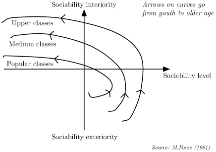
Figure 1: Evolution of the sociability of humans. As can be seen, the characteristics of one’s sociability are dependent on intrinsic personal characteristics, such as social class and age, instead of, e.g., the situation the person is in.

We base our proposal on the following findings. The first finding, intrinsicality, has been expressed concurrently in the literature by several research papers [14, 15]. It states that the sociability level of a given person is intrinsic to each person, and strongly dependent on internal factors (e.g., social class and age). This means that each individual has its own and constant sociability level at a given period in life that does not depend on its place in a social network – contrary to what one could assume – as shown by Fig. 1. This socialization level is translated to a need for social interactions. The second finding, interactivity, is derived from a socialization behavior defined in [16, 17], that assesses that individuals’ aim to fulfill their sociological interaction needs. This can be expressed by building new social ties until the needs are fulfilled or by satisfying these needs by encountering already known acquaintances. These acquaintances are defined by individuals to whom an individual is tightened in a social network.

Yet, social networks have already been used to design mobility models such as the ones proposed by Musolesi et al. [10, 19]. In these authors’ proposal, individuals are gathered in clusters by a heuristic which processes a graph representing social ties. Each cluster is then affected to a specific region in space. Mobility is generated by individuals moving from region to region according to a preferential attachment process. In a companion prior paper, we have already defined a mobility model based on this process [20]. Yet, as we will see in the next section, Musolesi et al.’s proposal and our model do not exploit the same social basis and hence differ in their expression and results.

III SIMPS: An interaction based mobility model

In this section, we present SIMPS in detail.

III-A Overview

SIMPS is a model of the social component of human motion. At the scale of a simulation, we assume: (i) fixed social interaction need per individual and (ii) fixed social graph representing social ties between individuals. Hence, the need of social interactions is satisfied by either encountering acquaintances or escaping from non-acquaintances. This requires that individuals meet through spatial displacements (mobility).

The interactions with acquaintances and non-acquaintances can be translated into a behavioral model. From these behaviors, defined by rules, individuals join and leave acquaintances. In SIMPS, each individual is associated with a personal sociability level, which is the equilibrium point of the social interaction volume she/he tries to achieve all the time. Each individual is also associated with a context-aware indicator, namely perceived surround, which indicates the individual’s perception of her/his current socialization volume; basically, this value depends on the number of surrounding individuals.

In order to meet the desired sociability level, individuals can resort to two complementary behaviors: socialize – movements toward acquaintances – and isolate – to escape from undesired presences. The acquaintances of an individual are determined by the social graph in which acquaintances are represented by directed edges. The effects of socialize and isolate behaviors are, respectively, to raise and lower one’s perceived surround. To activate one of these behaviors, a feedback decision process estimates, continually and for every individual, her/his current socialization volume, and compares it to the individual’s own needs.

SIMPS is composed of two parts: social motion influence and motion execution unit. The social motion influence updates an individual’s current behavior to either socialize or isolate. The motion execution unit is responsible for translating the behavior adopted by an individual into motion. We detail these processes in the following.

III-B Social motion influence

SIMPS simulates the dynamic properties of a population ${\mathcal{P}}$ containing $N$ individuals in a two-dimensional plane (although its expressions can be easily extended to more dimensions). Time $\tau$ is assumed to be discrete, with steps of $\Delta_{\tau}$.

Individual $i\in{\mathcal{P}}$ tends to socialize at her/his own volume, plus or minus a certain variation. This defines the following two random variables:

• $s_{i}$, or the sociability level of node $i$, is the number of individuals that node $i$ aims at being surrounded by.

• $t_{i}$, or the tolerance level of node $i$, is the fractional variation of the sociability level under which the individual still feels comfortable.

Following these random variables, we can define $i$’s social comfort range:

$$z_{i}=[s_{i}(1-t_{i}),s_{i}(1+t_{i})].$$ (1)

According to the theory of proxemics [21], the social awareness of an individual is situated in a sphere around her/him, whose radius $R_{soc}$, namely social distance, is approximately 3.5 meters, or 12 feet (cf., Section IV). In this sphere, the perception of nearby individuals is not immediate, i.e., individuals progressively notice the presence of others. Such a fuzzy perception is called the perceived surround, noted $u_{i}$. In order to reproduce this perception, in SIMPS, individual $i$’s perception is rendered by a pseudo-control loop as shown in Fig. 2. In this loop, the perceived surround $u_{i}$ is periodically mixed with $U_{i}(\tau)$, which gives the number of individuals within $i$’s social sphere at time $\tau$. The period of the pseudo-control loop is called half-perception time and noted $\tau_{r}$.

]Figures/ControlLoopHoriz.eps

Figure 2: Pseudo-control loop for the computation of the perceived surround.

We can now give expressions that determine the values of the different variables. Individual $i$’s surround is updated every $\tau_{r}$ seconds as follows:

$$u_{i}=\frac{U_{i}(\tau)+u_{i}}{2},$$ (2)

where $U_{i}(\tau)$ is given by:

$$U_{i}(\tau)=\sum_{\begin{array}[]{c}{\scriptstyle j=1}\\ {\scriptstyle j\neq i}\end{array}}^{n}P_{i,j}\textrm{, where }P_{i,j}=\left\{\begin{tabular}[]{l}$1$, if $|\overrightarrow{ij}|\leq R_{soc},$\\ $0$, otherwise.\end{tabular}\right.$$ (3)

In Eq. 3, $|\overrightarrow{ij}|$ denotes the Euclidian distance between nodes $i$ and $j$.

The perceived surround $u_{i}$ serves as input to the feedback decision process, which updates the behavior of the individual according to a sharp hysteresis as shown in Fig. 3. This hysteresis depends on both the individual’s sociability $s_{i}$ and tolerance level $t_{i}$.

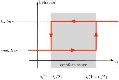
Figure 3: Sharp hysteresis curve for behavior decision process.

]./Figures/Tensions.eps

Figure 4: Illustration of the tension calculation process when the individual presents either socialize or isolate behaviors.

III-C The twin social behaviors

SIMPS also relies on social graphs from which motion influence behaviors are derived. Social graphs do not represent physical proximity, but only relationships among individuals. Nevertheless, the former influences the latter, since close acquaintances tend to get physically closer.

In SIMPS, a social graph $G=(V,E)$ is oriented and non-Eulerian. Vertices represent the nodes in the topology. Links, valuated in the range $[0;1]$, represent the acquaintances felt from its origin node toward its destination node: zero means no acquaintance at all (i.e., the destination is stranger to the origin) while one means high acquaintance (i.e., the destination has the maximum social proximity with the origin).

The acquaintance felt by $i$ toward $j$ is expressed as:

$$A_{i\to j}=\left\{\begin{tabular}[]{ll}$f(l_{i\to j})$&if $l_{i\to j}\in E$\\ $0$&otherwise,\\ \end{tabular}\right.$$ (4)

where $f(l)$ is the weight of edge $l_{i\to j}$.

Similarly, the strangeness $\overline{A_{i\to j}}$ felt by $i$ toward $j$ is defined as:

$$\overline{A_{i\to j}}=1-A_{i\to j}.$$ (5)

We can now precisely define the twin behaviors of nodes:

Definition 1

(Socialize) Individuals are attracted by acquaintances. The attractive tension $\overrightarrow{{\eta_{a}}_{ij}}$ felt by $i$ toward $j$ is a vector collinear to $\overrightarrow{ij}$, whose magnitude is proportional to the acquaintance $A_{i\to j}$ and inversely proportional to a power $\lambda$ of the distance $|\overrightarrow{ij}|$:

$$\overrightarrow{{\eta_{a}}_{ij}}=\frac{\hat{\overrightarrow{ij}}\,A_{i\rightarrow j}}{|\overrightarrow{ij}|^{\lambda}}\cdot$$ (6)

Definition 2

(Isolate) Individuals are repulsed by strangers. The repulsive tension $\overrightarrow{{\eta_{r}}_{ij}}$ felt by individual $i$ toward any other individual $j$ is a vector collinear to $\overrightarrow{ji}$, whose amplitude is proportional to the strangeness $\overline{A_{i\to j}}$ and inversely proportional to a power $\lambda$ of the distance $|\overrightarrow{ij}|$:

$$\overrightarrow{{\eta_{r}}_{ij}}=\frac{\hat{\overrightarrow{ji}}\,\overline{A_{i\rightarrow j}}}{|\overrightarrow{ij}|^{\lambda}}\cdot$$ (7)

The $\lambda$ parameter is called distance fading exponent.

Social motion influence. Nodes are either in socialize or isolate mode (as described in Section III-B). When in socialize mode, we have that $\overrightarrow{\eta_{ij}}=\overrightarrow{{\eta_{a}}_{ij}}$. On the other hand, when in isolate mode, node $i$ applies $\overrightarrow{\eta_{ij}}=\overrightarrow{{\eta_{r}}_{ij}}$. The vectorial sum $\overrightarrow{\eta_{i}}=\sum_{\scriptstyle i\neq j}\overrightarrow{\eta_{ij}}$ of all attractive or repulsive tensions give the direction of the willingness, $\overrightarrow{w_{i}}$, of $i$’s social motion influence (as depicted in Fig. 4.a and 4.b):

$$\overrightarrow{w_{i,\tau}}=\left\{\begin{tabular}[]{ll}$\hat{\overrightarrow{\eta_{i}}}e_{i,\tau}$,&if $\left|\overrightarrow{\eta_{i}}\right|\neq 0$,\\ $\overrightarrow{0}$,&otherwise,\end{tabular}\right.$$ (8)

where $e_{i,\tau}$, called $i$’s excitation, is given by:

$$e_{i,\tau}=\max\left(\left|\frac{u_{i}-s_{i}}{s_{i}t_{i}}\right|,1\right).$$ (9)

The excitation is null when $i$ feels surrounded at his exact sociability need $s_{i}$, and progressively increases until attaining $1$, when $i$’s surround $u_{i}$ falls outside $i$’s comfort range $z_{i}=[s_{i}(1-t_{i}),s_{i}(1+t_{i})]$.

A special instance of Eq. 8 happens when the sum of tensions is a null vector. Typically, this refers a situation where an individual is attracted toward many directions at the same time with a neutral result. In this situation, the individual hesitates and does not move. This situation, which is quite rare, is a case of instable equilibrium. The fact that neighboring individuals move makes this situation very short-lived.

III-D Motion execution unit

The social motion influence is not the sole parameter to have an impact on human motion. The role of the motion execution unit is to comply with two basic parameters governing the physical motion of individuals: velocity and acceleration. A more complete set of parameters (e.g., collision avoidance or terrain diversity) could be implemented; however, in order to focus on the social aspect of mobility, we only consider velocity and acceleration.

Velocities and accelerations are distributed according to two random variables, respectively $V$ and $A$, whose characteristics will be discussed later on. Individual $i$ is associated with an acceleration request, $\overrightarrow{{a_{r}}_{i,\tau}}$, which is proportional to $i$’s social motion influence:

$$\overrightarrow{{a_{r}}_{i,\tau}}={a_{\max}}_{i}\overrightarrow{w_{i,\tau}},$$ (10)

where ${a_{\max}}_{i}$ denotes the maximum scalar acceleration individual $i$ tolerates.

The acceleration request is applied with respect to $i$’s maximum velocity ${v_{\max}}_{i}$. Given $i$’s velocity vector at time $\tau-\Delta_{\tau}$, $\overrightarrow{v_{i,\tau-\Delta_{\tau}}}$, and the direction $\hat{\overrightarrow{{a_{r}}_{i,\tau}}}$ of the acceleration request, we compute the maximum acceleration $a_{lim_{i,\tau}}$ that can be applied for a duration $\Delta_{\tau}$ without trespassing ${v_{\max}}_{i}$. Since SIMPS discretizes time $\tau$ in steps of $\Delta_{\tau}$, we have:

$$\overrightarrow{v_{i,\tau}}=\overrightarrow{v_{i,\tau-\Delta_{\tau}}}+\overrightarrow{a_{i,\tau}}\Delta_{\tau}$$ (11)

and the speed limit condition:

$$\left|\overrightarrow{v_{i,\tau}}\right|\leq{v_{\max}}_{i}.$$ (12)

A short glance at Fig. 5 gives us:

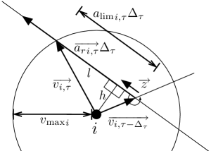
Figure 5: Calculation of ${a_{\lim}}_{i,\tau}$, in relation to $i$’s maximum velocity ${v_{\max}}_{i}$.

$$h=\left|\overrightarrow{v_{i,\tau-\Delta_{\tau}}}\right|\times\left|\sin\left(\widehat{\overrightarrow{{a_{r}}_{i,\tau}},\overrightarrow{v_{i,\tau-\Delta_{\tau}}}}\right)\right|,$$ (13)

$$l = \sqrt{{v_{\max}}_{i}^{2}-h^{2}}=$$

$$= \sqrt{{v_{\max}}_{i}^{2}-{\left(\left|\overrightarrow{v_{i,\tau-\Delta_{\tau}}}\right|\times\left|\sin\left(\widehat{\overrightarrow{{a_{r}}_{i,\tau}},\overrightarrow{v_{i,\tau-\Delta_{\tau}}}}\right)\right|\right)}^{2}}$$

and the projection of $\overrightarrow{z}$ on $\overrightarrow{{a_{r}}_{i,\tau}}$:

$$z=\left|\overrightarrow{v_{i,\tau-\Delta_{\tau}}}\right|\times\left(-\cos\left(\widehat{\overrightarrow{{a_{r}}_{i,\tau}},\overrightarrow{v_{i,\tau-\Delta_{\tau}}}}\right)\right).$$ (15)

We have that:

$${a_{\lim}}_{i,\tau}\Delta_{\tau}=h+z.$$ (16)

We can then obtain:

$${a_{\lim}}_{i,\tau} = \frac{\sqrt{{v_{\max}}_{i}^{2}-{\left(\left|\overrightarrow{v_{i,\tau-\Delta_{\tau}}}\right|\times\left|\sin\left(\widehat{\overrightarrow{{a_{r}}_{i,\tau}},\overrightarrow{v_{i,\tau-\Delta_{\tau}}}}\right)\right|\right)}^{2}}}{\Delta_{\tau}}$$ (17)

$$-\frac{\left|\overrightarrow{v_{i,\tau-\Delta_{\tau}}}\right|\times\cos\left(\widehat{\overrightarrow{{a_{r}}_{i,\tau}},\overrightarrow{v_{i,\tau-\Delta_{\tau}}}}\right)}{\Delta_{\tau}}$$

The acceleration request is then satisfied at best by the final acceleration $\overrightarrow{a_{i,\tau}}$:

$$\overrightarrow{a_{i,\tau}}=\hat{\overrightarrow{{a_{r}}_{i,\tau}}}\times\min\left(\left|\overrightarrow{{a_{r}}_{i,\tau}}\right|,{a_{\lim}}_{i,\tau}\right),$$ (18)

which is used to update $i$’s current velocity $\overrightarrow{v_{i,\tau-\Delta_{\tau}}}$ and position $\overrightarrow{p_{i,\tau}}$:

$$\left\{\begin{tabular}[]{l}$\overrightarrow{v_{i,\tau}}=\overrightarrow{v_{i,\tau-\Delta_{\tau}}}+\overrightarrow{a_{i,\tau}}\Delta_{\tau}$,\\ $\overrightarrow{p_{i,\tau}}=\overrightarrow{p_{i,\tau-\Delta_{\tau}}}+\overrightarrow{v_{i,\tau}}\Delta_{\tau}$.\end{tabular}\right.$$ (19)

IV Evaluation

Table I summarizes the parameters that are internal to the SIMPS mobility generator. They are described in the following.

TABLE I: Parameters used by SIMPS.

Name	Relates to	Type	Description	Value	Investigated
$V$	Pedestrian motion	Random variable	Maximal speed of individuals	$N(\mu=1.34,\delta^{2}=0.26)$	No
$A$	Pedestrian motion	Random variable	Maximum acceleration of individuals	$N(\mu=1.3,\delta=0.4)$	No
$S$	Sociability	Random variable	Sociability of individuals	$N(\mu=2.5,\delta=1)$	Yes
$T$	Sociability	Random variable	Tolerance of individuals	Uniform in $[0.1;0.7]$	No
$N$	Social graph	Integer variable	Number of nodes/individuals	$\in\mathbb{N}$	Yes
$D$	Social graph	Real variable	Average node outdegree	$\in[0;N-1]$	Yes
Graph type	Social graph	Enumerated value	Graph type	in {Natural,Random,Scale-Free}	Yes
$R_{soc}$	Human perception	Real variable	Social radius	$3.5$ meters	Yes
$\tau_{r}$	Human perception	Real variable	Half-perception time	$4$ seconds	Yes
$\lambda$	Human perception	Real variable	Distance fading exponent	$\in[0;3]$	Yes
Space	Space	Enumerated value	The space where motion happens	in {Infinite, Periodic Square}	Yes
$L$	Space	Real variable	Size of periodic shape	$\in[0;+\infty[$	Yes
$\tau_{\max}$	Time	Real variable	Total time considered	$\in[0;+\infty[$	Yes
$\Delta_{\tau}$	Time	Real variable	Time quantization step	$\in[0;\tau_{\max}[$	Yes

IV-A Pedestrian motion characteristics

This parameter dictates the distributions of the random variables $V$ and $A$, respectively the velocity and acceleration of the individuals. According to results published by Henderson in [22], velocity $V$ for pedestrians is set to follow a normal law $N(\mu=1.34,\delta^{2}=0.26)$. Acceleration distribution is harder to gauge. Considering that a human can switch from immobile position to walking in the order of the second, we empirically set it to follow a similar normal law $N(\mu=1.3,\delta^{2}=0.4)$.

IV-B Social interactions characteristics

These characteristics govern the interactions between individuals. Random variables $S_{i}$ and $T_{i}$, introduced in Section III-B, denote, respectively, the volume of social interaction required by each individual (sociability) and the variation she/he tolerates on this volume of interaction (tolerance). To assess $S_{i}$, we look into the group size distribution found in [22]. The results are expressed as a Poisson law ($\lambda=2.5$) of discrete values. Since the sociability distribution in SIMPS is a continuous function, we translate the discrete Poisson law into a normal law $N(\mu=2.5,\delta^{2}=1)$, for which we investigate in this paper the effect of variation of its first moment. Furthermore, the tolerance on this sociability is set to a uniform distribution in $[0.1;0.7]$ (i.e., between $10\%$ and $70\%$ tolerance on the sociability).

The social graph defines acquaintances between individuals, which are used to compose the twin behaviors. This graph is parameterized by the number of nodes, $N$, the average node degree $D$, and the type, which can be natural (when drawn from real traces) or synthetic (e.g., Erdös-Rényi random graph, exponential node-degree distributed graph, or Albert-Barabási scale-free graph with power-law node degree distribution). Average node degree for various measured social graphs vary more than one order of magnitude depending on the subject of the social graph. For example, sexual contact graphs exhibit a low average node degree ($D\approx 2$), followed by phone calls graphs ($D\approx 3$), blogs ($D\approx 14$), up to actor collaboration ($D\approx 61$). Since nodes in the graph represent mobile individuals, the size of the graph gives the population size to which the random variables $V$, $A$, $S$, and $T$ apply.

IV-C Human perception characteristics

This parameter defines the way human beings perceive their environment. They are in number of three: social distance, half-perception time, and distance fading exponent. Proxemics, defined by E. T. Hall [21], stipulates that relations between humans are dependent on the distance separating them. The social distance is the physical distance under which social transactions and interactions occur. In the United States, this distance was measured to be around $12$ft. (or $3.5$m); however, this value was found to vary from about half to several times this distance, depending on cultural variations, and also on spatial constraints, such as typically crowded areas. In SIMPS, this value is directly translated into $R_{soc}$, the distance used for one’s current socialization estimation. While $3.5$m is the typical value we set for our tests, we also investigate the impact of its variations.

The half-perception time $\tau_{r}$ regulates the pseudo-control loop described in Section III-B. It describes the time an individual takes to perceive changes in her/his neighborhood. Although, to our knowledge, this parameter has not been much investigated, some documents in the literature show that the perception time may range from hundreds of milliseconds to tens of seconds [23, 24]. SIMPS is about pedestrian motion, which is a more relaxed environment; in such a context, users spend more time to react, and reaction times are considered in the order from around one second to tens of second.

One of the particularities of physical motion is that each movement has a cost. In SIMPS, this is taken into account by the distance fading exponent $\lambda$ (cf., Section III-C), which defines the cost an individual associates to the distance that separates her/him from another individual. Basically, when $\lambda=1$, it means that the distance has a first order impact on the result (the cost of a motion is considered linear to the distance), while $\lambda=2$ means that the distance has a second order impact (the cost is considered to be in square of the distance). In Section VI, we will investigate $\lambda$ in detail.

IV-D Spatial characteristics

This parameter describes the space in which individuals evolve. The boundary conditions can be of three types: infinite, finite, and periodic. If finite, the topology can be a square, a hexahedron, a disc, a bitmap, or a parametric space given by a twin set of polygons (presence zone polygons minus obstacle polygons). If periodic, the topology can be a square (with toroidal boundary mapping), a set of hexahedrons (with cell-like boundary mapping), or a pair of discs (with bi-hemispheric boundary mapping). In the remainder of this paper, we investigate the properties exhibited by SIMPS alone. Aiming at the simplest scenarios, we will restrict our study to the infinite and periodic square (toroidal mapping) cases, in which the influence of square side $L$ will be investigated.

IV-E Time characteristics

Time characteristics concern the total duration $\tau_{\max}$ for which motion is considered, and the time quantization step $\Delta_{\tau}$ used for motion rendering. These two values, although more related to implementation than to model definition, are of prime concern since their choice can directly influence the outcome of the synthesized motion. It is then of major importance to distinguish inherent characteristics of our model from eventual effects on its outcomes due to time sampling. In the analysis below, we explore the effect of time quantization and total considered duration on the results of SIMPS.

V Methodology

In this section, we wish to highlight the outcome of our approach, which comforts recent observations of power-laws. The most common observation of power-law distributions lies in the contact/inter-contact durations. It is exhibited by studies conducted on WiFi-enabled devices at ETH Zurich, Dartmouth, and UCSD. Recently, a specific set of experiments conducted by Cambridge University, UK, in collaboration with Intel, traced the contact and inter-contact duration distributions between mobile users carrying iMotes Bluetooth devices [6]. Although at a lower communication scale than previous studies, the three experiments conducted in [6] (all three at different times and locations, and with different users) showed strikingly similar observation of the scale-free characteristics of human contacts. Contact and inter-contact durations have been observed to follow power laws whose exponents were situated respectively around $-1.5$ and $-0.6$, with cut-offs related to the durations of the observations.

In order to investigate social interactions between individuals, we simulate human mobility with conditions similar to [6]. In the iMotes experiments, users carried Bluetooth-enabled devices, which periodically recorded the presence of other BlueTooth-enabled devices, such as other iMotes, PDAs, mobile phones, or laptops. A contact situation between individuals was asserted as soon as the presence of one node was felt by the other one, and an inter-contact asserted as soon as two or more consecutive measures did not show the presence of a previously seen node. The theoretical range of BlueTooth is around $10$ meters. We consider however that a more realistic $6$-meter range is a valid assertion for sensing range in most situations. In this way, we chose to simulate a simplistic range-based contact condition based on a maximum distance of $6$ meters separating individuals.

TABLE II: Summary of test settings.

Aspect	$\Delta_{\tau}$	$\tau_{max}$	$\left<S\right>$	Graph type	$D$	$\lambda$	$R_{soc}$	Space	$L$	$\tau_{r}$
Social graph type	$1$s	$3600$s	$2.5$	$[$Random,SF$]$	$5$	$1$	$3.5$m	Periodic	$200$m	$4$s
Avg. node degree	$1$s	$3600$s	$2.5$	Scale-Free	$[2,5,15,50]$	$1$	$3.5$m	Periodic	$200$m	$4$s
Sociability	$1$s	$3600$s	$[1,2.5,10]$	Scale-Free	$5$	$1$	$3.5$m	Periodic	$200$m	$4$s
Socialize only	$1$s	$3600$s	$2.5$	Scale-Free	$5$	$1$	$0$	Periodic	$200$m	$4$s
Isolate only	$1$s	$3600$s	$0$	Scale-Free	$5$	$1$	$>\sqrt{2}\times L$	Periodic	$200$m	$4$s
Social distance	$1$s	$3600$s	$2.5$	Scale-Free	$5$	$1$	$[1,3.5,15]$m	Periodic	$200$m	$4$s
Reaction time	$1$s	$3600$s	$2.5$	Scale-Free	$5$	$1$	$3.5$m	Periodic	$200$m	$[1,4,20]$s
Distance cost	$1$s	$3600$s	$2.5$	Scale-Free	$5$	$[0,1,2,3]$	$3.5$m	Periodic	$200$m	$4$s
Space: infinite	$1$s	$3600$s	$2.5$	Scale-Free	$5$	$1$	$3.5$m	Infinite	$\infty$	$4$s
Space: periodic	$1$s	$3600$s	$2.5$	Scale-Free	$5$	$1$	$3.5$m	Periodic	$[20,200,2000]$m	$4$s
Total duration	$1$s	$[600$s$,1$h$,10$h$]$	$2.5$	Scale-Free	$5$	$1$	$3.5$m	Periodic	$200$m	$4$s
Time quantization	$[0.1,1,10]$s	$3600$s	$2.5$	Scale-Free	$5$	$1$	$3.5$m	Periodic	$200$m	$4$s

VI Results and discussion

Tests on the outcome of SIMPS mobility regarding contact and inter-contact distributions have been conducted over a population of $N=100$ individuals. The general parameters used by SIMPS are shown in Table II while the different values of the simulations we conducted are depicted in Table I.

VI-A Influence of social graph

Figure 6: Effect of the underlying graph on the outcome of the SIMPS mobility. Contact and inter-contact duration distributions taken with two inputs: Albert-Barabási scale-free graph with power law node degree distribution and Erdös-Rényi random graph with exponential node degree distribution.

The first aspect to gauge is the behavior of the model in the general case, and its dependence with the underlying graph structures. To this effect, the distributions of contact and inter-contact durations of Bluetooth-carrying nodes subject to SIMPS mobility are plotted, for both random and scale-free graphs, in Fig. 6. As we can observe, the contact and inter-contact duration distributions follow power-laws in both cases, and with very close exponents. The distribution of inter-contact is a bit below the one of the scale-free graph, while contact duration distributions are very close for both graph structures. All these distributions experiment an exponential cut-off around $500$ seconds. As will be seen later on, these cut-offs are due to the duration of the simulation.

The similarity of the mobility patterns obtained with scale-free and exponential graphs is noticeable, and both correspond to the same power law of exponent $\alpha=1.2$. Inter-contact distributions are also very similar for both graph types, with a slightly sharper cut-off for the scale-free social graph. We conclude from this that the graph structure has minor influence relatively to the emergence of the power-law contact and inter-contact distributions. This result is very important and surprising: although social graph are notable for their scale-free degree distribution, scale-free contact and inter-contact distributions are not due to this feature, and emerges from the social motion.

Figure 7: Effect of the variation of average node degree $D$ on the outcome of SIMPS.

The average node-degree $D$ of the social graph can vary significantly depending on the scenario. We verify then how SIMPS behaves under different average node degrees. Tests have been run for four different values of $D$: $2$, $5$, $15$, and $50$. These values span a broad range of situations encompassing most social graphs studied in literature. The results are plotted in Fig. 7. We observe that contact and inter-contact distributions remain quite stable in their power-law nature, despite the important changes in the underlying social graph. The exponents in both distributions tend to increase slightly in function of $D$.

The two previous observations give us high confidence in the robustness of SIMPS, and its reasonable independence relatively to the social graph used. For this reason, we decide to use Albert-Barabási scale-free social graphs for the remainder of this paper. These are considered to be closer to real social graphs than Erdös-Rényi random graphs. The default $D$ value used, unless needed otherwise, will be $5$.

VI-B Influence of sociability

Figure 8: Effect of the average sociability on the outcome of the SIMPS mobility, for contact and inter-contact duration distributions of mobile nodes carrying Bluetooth-like devices.

The next parameter we must verify for a social model is the variation of the social influence. We performed tests for three different values of $\left<S\right>$, the first moment of random variable $S$, for which the distributions are shown in Fig. 8. We can see from the graph that although the slope of both distributions change with the settings, their nature remains as a power-law with cut-off. For larger values of $\left<S\right>$, in which humans have higher needs for socialization, the inter-contact distribution changes the most. This is an important phenomenon that we will explore hereafter: the power-law nature of both distributions outputted by SIMPS seems strictly dependent on the balanced presence of both socialize and isolate behaviors.

VI-C Separate effects of socialize and isolate behaviors

Figure 9: Separate effect of socialize and isolate behaviors on SIMPS results.

We evaluate now the contribution of each of the twin social behaviors on mobility. To this end, we set the model for three runs. The first considers only the socialize behavior, the second considers only the isolate behavior, and the third considers both behaviors together. Setting a single behavior is accomplished by changing $R_{soc}$, the social distance (defined in Section III-B). Setting $R_{soc}=0$ means that individuals always want to socialize. Setting $R_{soc}>\sqrt{2}\times L$ and distributing $S$ and $T$ so as no individual tolerates a surround of more than $N-1$ individuals imposes that all individuals will feel over-socialized and want to isolate. The corresponding results are shown in Fig. 9.

We can observe from the graph the clear influence of the isolate behavior on the power-law distribution. Both contact and inter-contact duration distributions exhibit neat scaling laws. It is however not sufficient to explain the strong exponent difference between these two distributions, characteristic of all observations. The outcome of the socialize behavior is by far the more interesting – inter-contact distribution is far below contact distribution, and follows two power law sections separated by a sudden decrease. Such a staircase-like feature could explain the presence of two smaller bumps barely visible as an outcome of SIMPS, and also present in various real-life measures, such as in [6]. In order to ensure that these bumps were not the result of the periodic space used, an additional run has been performed in an infinite space. The results exhibit the same characteristic. Another interesting emergent behavior is that, although individuals are most of the time in socialize mode, the global outcome of SIMPS tends more toward the characteristics exhibited by the isolate behavior. This seems to indicate that the mixture of both behaviors is very different from their average, hence pointing the emergence of a different mechanism from their interplay.

VI-D Influence of human perception

Figure 10: Effect of the social distance on SIMPS outcome.

VI-D1 Social distance

Human perception also has direct influence on mobility. As discussed earlier in this paper, the typical social distance $R_{soc}$ between human beings was found to be around $3.5$ meters for U.S. citizens [21], subject to variations depending on sociocultural background (e.g. smaller in Latin countries, bigger for rural areas) and context (e.g. reduced in crowded areas, sport events). In order to assess the effect of perception on mobility, a test has been run with 3 different values of $R_{soc}$: $1$ m, $3.5$ m, and $15$ m. The results are shown in Fig. 10.

As seen with the case where $R_{soc}$ is reduced to $1$ m, contact and inter-contact duration distributions still show a power-law feature with cut-off, but with a higher exponent. When $R_{soc}$ is raised to $15$ m, both distributions experience a slight decrease in its exponent; however, the cut-off arrives much sooner in the contact distribution. This might be due to border effects, when the size of the social sphere approaches the total space considered for mobility (as we will see in Section VI-E). While interesting for our study, it is unlikely that this extreme case happens in reality, since proxemics states that the variation of social distance is related to the context an individual is immersed into; for instance, social distance is reduced in crowded areas.

Figure 11: Effect of the half-perception time on SIMPS outcome.

VI-D2 Half-perception time

We now investigate the impact of how quick human beings perceive changes in their immediate surroundings. We performed tests with three possible value of the half-perception time, $\tau_{r}$: $1$ s, $4$ s, and $20$ s. The results are shown in Fig. 11.

Although all values of $\tau_{r}$ lead to close results, we note two tendencies. On the one hand, when perception time is minimal, the inter-contact distribution exhibits lower values, but more frequently. This is in part due to the fact that individuals rapidly try to escape from crowds and come back to meet acquaintances. A similar observation can be drawn for the contact distribution, but with lower impact. On the other hand, when perception time is at the longest bound, inter-contact distribution does not change that much, while contact distribution shows a neat decrease in the proportion of shorter contacts.

It finally appears that the half-perception time of $4$ s (chosen for the rest of our simulations) does not lead to any of the border effects observed above. It results in strict power-laws and clear distinction between contact and inter-contact distributions, which are closer to the results obtained by Chaintreau et al. [6].

Figure 12: Effect of the distance-associated cost estimation on SIMPS outcome.

VI-D3 Distance fading exponent $\lambda$

One of the particularities of physical motion is that each movement has a cost. In SIMPS, this is taken into account by the distance fading exponent, $\lambda$, which is used by each individual to weight the interest of meeting/avoiding another individual relatively to the distance separating them.

We ran tests with four different values of $\lambda$: $0$ (distance has no influence on attraction between individuals), $1$ (distance plays linearly), $2$ (distance plays as a square), and $3$ (distance plays as a cube). The results are shown in Fig. 12. The main outcome of these tests is that when distance is not taken into account ($\lambda=0$), mobility is mainly characterized by a Weibull distribution, instead of a power-lay. While still showing scale-invariance in time, Weibull distributions are less characteristic of empirical traces, which tend more to a power-law.

Furthermore, the order at which distance is used in cost estimation does not fundamentally change the outcomes of SIMPS. The results indicate that distance plays a direct role in human displacement decisions, confirming results shown in [20].

VI-E Influence of the simulation space

Figure 13: Effect of the considered space on SIMPS results.

Individuals present different mobility characteristics depending on the space they evolve in. We explore here two parameters defining motion space. The first one, namely space type, defines if individual evolve in free, limited, or periodic space. In the case of limited space, two options can be considered to manage the situation where individuals attain a border: (a) nodes stop when they face a border (obstruction); (b) nodes’ directions are symmetrically reflected against limits (reflection). In periodic spaces, these latter are considered as a torus – nodes escaping one border are replaced in the opposite border of the space. This model has the advantage of leading to regular average spatial density.

Contrary to the experiments described earlier in this paper, which ran over periodic spaces, we consider now more realistic free spaces. The goal is to investigate if our observations still hold. In addition, in the case of a non-infinite space, we also consider the impact of the density on the results, since it directly influences the equilibrium between the quantities of socializing and isolating individuals. We vary density with the inverse square of side $L$. The first run is performed in free-space, with users initially uniformly disposed in a square of 200 m on side, while the other simulations are performed in a periodic square space with sides varying between $20$ m and $2,000$ m. The results are shown in Fig. 13.

The first observation is that in the free-space case contact and inter-contact distributions exhibit very close power-laws. This is a reminiscent characteristic of the isolate behavior – individuals can take the entire place they want. Looking at the runs with periodic space, the evolution of the distributions suggests a specific value of density that corresponds to the point of equilibrium between socialize and isolate behaviors. Above this point, the results tend to an exponential law, which is an inheritance of the RWP model. This is probably due to the fact that individuals move quickly from a point to another, and all the conditions change dramatically from one simulation step to another, rendering senseless the decisions of social adaptation. Below the point of equilibrium, the results obtained with a periodic space tend to approach the ones of free space.

VI-F Influence of considered time

The influence of time on SIMPS outcomes appears in two ways: time quantization step and total simulation time. The first aspect is related to the very common problem of sampling on measurements. It can be summarized in one simple question: “Is the considered time step fine enough for a realistic view of the system?” To explore this issue, we ran three tests, with times quantization steps of $0.1$ s, $1$ s, and $10$ s, respectively. The results are shown in Fig. 14.

Figure 14: Effect of the time quantization step on SIMPS results.

It is straightforward to observe that the results with $\Delta_{\tau}=0.1$ s and $\Delta_{\tau}=1$ s are very close one to the other, while $\Delta_{\tau}=10$ s completely changed the results. We can consider then with confidence that a time discretization step of $1$ s is fine enough for the results we wish to observe. Such a time granularity is in accordance with the half-perception time of $\tau_{r}=4$s we identified in our earlier experiments, and with the precept that a human goes from steady-state to full motion or inversely in around $1$ s (recall that this value was used for acceleration distribution).

Figure 15: Effect of the total duration considered on SIMPS results.

The second important aspect related to the influence of time is the total duration of the simulation, since it directly influences the cut-off in the tail of the distributions. The fundamental question here is: “Do these observations extend with time considered, or are they limited in scale?” Again, three tests were conducted, with total durations of $\tau_{\max}~{}=600$ s, $\tau_{\max}=3,600$ s, and $\tau_{\max}=36,000$ s. The results are shown in Fig. 15. As expected, the cut-offs are shifted right or left depending on the duration of the simulation. This comforts theoretical results that mobility contact and inter-contact distributions are purely power-law in essence.

VII Further discussion

VII-A About complex systems modeling

The main discussion relative the modeling of complex systems lies in the differences between two approaches:

• Simple models with mathematically tractable parameters should be preferred whenever possible, since their use allows obtaining strict results and deterministic predictions.

• More complex models, on the other side, often tend to be non-deterministic and only render empiric results, on smaller parameter ranges, with stochastic conditions.

The advantages in terms of “realism” of the latter approach is often considered dubious, when simpler models might render similar predictions. Indeed, a complex model is only interesting when it explores situations to which deterministic models cannot apply. With these considerations in mind, we aimed at making SIMPS as simple as possible, though exhibiting complex emerging features. Although SIMPS could be made more complex and specialized in many manners (for example, by introducing a third behavior stating that an individual just pauses at some location), we believe that such additions would restrict the scope of our results. Such adaptations, however, are welcome in more specific situations.

We also believe that SIMPS brings novelty in two ways: (a) it adapts outer knowledge from sociology that has not been used before and (b) it generates mobility patterns that spans a wide range of empirical observations in an extremely robust fashion.

VII-B About complex behavior emergence

The combination of very simple interacting rules leads sometimes to very complex outputs. Such an emergence phenomenon can be observed for instance via the SIMPS front-end interface (a real-time graphical interface of the simulator). We can observe for example situations referred to as bugger’s case: an isolating node closely pursued by a socializing node. This appears as pairs of nodes having a highly asymmetric social relation. Further observations showed that such situations resolve themselves since they are part of a more complex collective mechanism.

VIII Conclusion

In this paper, we proposed SIMPS, a new mobility model that addresses the roots of mobility. SIMPS deals with sociological influences in human crowd motion found in typical situations like malls, fairs, cafeterias, clubs, beaches, or fora. SIMPS’s modular conception separates motion influences from motion generation, which allows associating additional mobility influences with little effort. Based on a human feature thoroughly studied in sociology, namely sociability, SIMPS defines two behaviors that regulate each individual’s social interaction level.

We evaluated SIMPS using a simple in-range contact model. Under the light of recent measures of contact and inter-contact duration distributions, we draw the following surprising conclusions from our study:

• Although entirely synthetic, SIMPS’s traces show strong similarities with various heavy-tailed distributions observed in real-life situations.

• Such heavy-tailed features are emergent. While SIMPS uses a social graph for estimating motion, we show that the graph structure has negligible influence on the results. Decomposing the influence of the graph into two complementary behaviors, namely socialize and isolate, we show the crucial role of their interplay in the final mobility pattern.

• The investigation of some input parameters seems to bring clues on the occasional tendency of contact and inter-contact distributions to show Weibull distribution characteristics.

References

- [1] J.-Y. Le Boudec and M. Vojnovic, “Perfect simulation and stationarity of a class of mobility models,” in IEEE INFOCOM, Miami, FL, Mar. 2005.
- [2] A. Jardosh, E. Belding-Royer, K. Almeroth, and S. Suri, “Real world environment models for mobile ad hoc networks,” IEEE Journal on Selected Areas in Communications, vol. 23, no. 3, Mar. 2005.
- [3] A. K. Saha and D. Johnson, “Modeling mobility for vehicular ad hoc networks,” in ACM Workshop on Vehicular Ad Hoc Networks (VANET), Philadelphia, PA, July 2004.
- [4] C. Bettstetter, “Smooth is better than sharp: a random mobility model for simulation of wireless networks,” in ACM MSWiM, Rome, Italy, July 2001.
- [5] D. Choffnes and F. Bustamante, “An integrated mobility and traffic model for vehicular wireless networks,” in ACM Workshop on Vehicular Ad Hoc Networks (VANET), Cologne, Germany, Sept. 2005.
- [6] A. Chaintreau, P. Hui, J. Crowcroft, C. Diot, R. Gass, and J. Scott, “Impact of human mobility on the design of opportunistic forwarding algorithms,” in IEEE Infocom, Barcelona, Spain, Apr. 2006.
- [7] D. Kotz and K. Essien, “Analysis of a campus-wide wireless network,” in ACM Mobicom, Atlanta, GA, Sept. 2002.
- [8] M. McNett and G. Voelker, “Access and mobility of wireless PDA users,” Mobile Computing and Communications Review, vol. 9, no. 2, pp. 40–55, Apr. 2005.
- [9] C. Tuduce and T. Gross, “A mobility model based on WLAN traces and its validation,” in IEEE Infocom, Miami, FL, Mar. 2005.
- [10] M. Musolesi, S. Hailes, and C. Mascolo, “An ad hoc mobility model founded on social network theory,” in ACM MSWim, Venice, Italy, Oct. 2004.
- [11] M. Grossglauser and D. Tse, “Mobility increases the capacity of ad hoc wireless networks,” IEEE/ACM Trans. on Networking, vol. 10, no. 4, pp. 477–486, Aug. 2002.
- [12] B. Zhou, K. Xu, and M. Gerla, “Group and swarm mobility models for ad hoc network scenarios using virtual tracks,” in IEEE Milcom, Monterey, CA, Oct. 2004.
- [13] W. Hsu, K. Merchant, H. Shu, C. Hsu, and A. Helmy, “Weighted waypoint mobility model and its impact on ad hoc networks,” ACM Mobile Computer Communications Review (MC2R), vol. 9, no. 1, pp. 59–63, Jan. 2005.
- [14] M. Forsé, “Les réseaux de sociabilité dans un village,” Population (French Edition), vol. 36, no. 6, pp. 1141–1162, Nov. 1981.
- [15] R. Laporte, “Pratiques sportives et sociabilité,” Journal of Mathematics and Social Sciences, vol. 43, no. 170, pp. 74–94, Nov. 2005.
- [16] T. Snijders, “The statistical evaluation of social network dynamics,” Sociological Methodology, 2001.
- [17] ——, Models for Longitudinal Network Data. New-York: P. Carrington, J. Scott, & S. Wasserman (Eds.), Cambridge University Press, 2005.
- [18] X. Hong, M. Gerla, G. Pei, and C. Chiang, “A group mobility model for ad hoc wireless networks,” in ACM/IEEE MSWiM, Seattle, WA, Aug. 1999.
- [19] M. Musolesi and C. Mascolo, “A community based mobility model for ad hoc network research,” in ACM/SIGMOBILE International Workshop on Multi-hop Ad Hoc Networks: from theory to reality (REALMAN), Florence, Italy, May 2006.
- [20] V. Borrel, M. D. de Amorim, and S. Fdida, “A preferrential attachment gathering mobility model,” IEEE Communications Letters, vol. 9, no. 10, pp. 900–902, Oct. 2005.
- [21] E. Hall, The Hidden Dimension. Garden City, N.Y.: Doubleday, 1966.
- [22] L. Henderson, “The statistics of crowd fluids,” Nature, no. 229, pp. 381–383, Feb. 1971.
- [23] A. Welford, Reaction Times. New-York: Academic Press, New York, 1980.
- [24] T. Triggs and W. Harris, “Reaction time of drivers to road stimuli,” Monash University Human Factors Group - Report HFR-12, Tech. Rep., 1982.