About the Lifespan of Peer to Peer Networks

Abstract

In this paper we analyze the ability of peer to peer networks to deliver a complete file among the peers. Early on we motivate a broad generalization of network behavior organizing it into one of two successive phases. According to this view the network has two main states: first centralized - few sources (roots) hold the complete file, and next distributed - peers hold some parts (chunks) of the file such that the entire network has the whole file, but no individual has it. In the distributed state we study two scenarios, first, when the peers are “patient”, i.e, do not leave the system until they obtain the complete file; second, peers are “impatient” and almost always leave the network before obtaining the complete file.

We first analyze the transition from a centralized system to a distributed one. We describe the necessary and sufficient conditions that allow this vital transition. The second scenario occurs when the network is already in the distributed state. We provide an estimate for the survival time of the network in this state, i.e., the time in which the network is able to provide all the chunks composing the file. We first assume that peers are patient and we show that if the number of chunks is much less than $e^{n}$, where $n$ is the number of peers in the network, then the expected survival time of the network is exponential in the number of peers. Moreover we show that if the number of chunks is greater than $\frac{\log n}{n+1}e^{n+1}$, the network’s survival time is constant. This surprisingly suggests that peer to peer networks are able to sustain only a limited amount of information. We also analyze the scenario where peers are impatient and almost always leave the network before obtaining the complete file. We calculate the steady state of the network under this condition. Finally a simple model for evaluating peer to peer networks is presented.

Keywords: P2P, file sharing, chunk, downloading rate, survivability

1 Introduction

Over recent years, peer to peer (P2P) networks have emerged as the most popular method for sharing and streaming data (see for instance [1]). There has been popular adoption and widespread success due to the high efficiencies that these networks obtain for broadcast data. Apart from personal usage, many companies, like for instance redhat_®, provide links in order to download their free distributions in a P2P fashion. In doing so, companies avoid the problem of too many clients connected to their server. This solves bottleneck or high concentrated transmission cost on a single node with a significant chance of failure at peak loads. On the other hand, companies are not the only benefactor. Indeed, it makes things much faster from the point of view of the user even though at the expense of “being used” by other users.

Another very interesting application where such networks are highly successful concerns the distribution of data for storage purposes. The idea, in fact, to collect data among users spread over all the world is increasing more and more. Instead of having (for each one) a full copy of everything, a community can share resources hence obtaining a distributed storage device. This permits them to collectively maintain more and more data and it increases also the reliability. It ensures, in fact, that data will not disappear due to the malfunction of a small number of devices.

The main differences among the two applications we have just outlined are a more collaborative environment and a lower percentage of disappearing pieces of data, with the second being the more reliable in this sense. For downloading purposes, in fact, the aim is sometimes to download the required data as fast as possible and then leave the network. This implies also a higher frequency in peers disappearing. On the other hand, in an ideal world where people collaborate for a common final purpose, we like to imagine both the applications are quite equivalent.

We consider the following processes. A file is divided into $k$ chunks. The network contains a large number of nodes. We distinguish among peers, i.e., nodes with a number of chunks less than $k$ and roots, i.e., nodes owning all the chunks. We assign to peers a probability $\alpha$ for which they may disappear. This means that peers live on average $\frac{1}{\alpha}$ rounds. For the roots we chose a probability $\alpha_{R}\geq\alpha$. We consider closed network, i.e., every time a peer or a root leaves the network a new peer will join with no chunks. For the sake of simplicity we consider a synchronous model. During a round each node can receive or send one chunk; and at the end of each round any node disappears with respect to the related probability. We study the following three scenarios:

Spreading or Centralized Scenario: Peers contain no chunks and there are $R$ roots. We wonder if the file is spread into the network. This happens if all the chunks are sent from the roots inside the network where they multiply themselves. This can give us a measure for the file length with respect to the life of the last surviving root. After the last root leaves the network, in fact, either the file has been spread or it is not possible to build it back. We say in this case, the network (or the file) is “dead”.

Distributed Scenario: The chunks are widely spread in the network. There is not a fixed amount of roots, $R$ can be also zero, we only require that the whole chunks composing the file are there. We wonder if the network life is long or short. As we are going to see, the network life is long when some almost steady state is reached. This can give us a measure about the conditions ensuring a long life for the network, and, when this happens, how often a full download is completed.

Survivability Scenario: In this scenario we are interested in studying the network behavior under extreme conditions. We consider, in fact, the case in which a file is almost never downloaded since peers have a very high volatility. They almost never stay in the network long enough to perform a full download. However, it is still very interesting to note that the network is able to survive. We recall that a network is said to survives whenever it still contains all the $k$ chunks composing the original file, no matter where they reside.

Given some parameter settings, our aim is to answer the question of how long we can expect a network to continue producing new completed downloads. For all the previous three scenarios we provide a stochastic formulation. We show how parameters should be set up in order to obtain the desired results concerning network survivability and file downloading rate. It turns out that the eventual fate of the network is mainly dependent on the number of nodes $n$ and the number of chunks $k$ in which the file is split. We show how the network may pass through the previous three scenarios before eventually dying.

1.1 Related Work

A lot of work has been devoted to the area of file sharing in P2P networks. Many experimental papers provide practical strategies and preliminary results concerning the behavior of these kind of networks. In [2] for instance, the authors essentially describe properties like liveness and downloading rate by means of extended experiments and simulations under several assumptions.

Concerning analytical models it is very difficult to capture suitable features in order to describe what happens and why protocols like BitTorrent [3] are so powerful in practice. Suitable models are hard to find that describe what sometimes is easily observable by simulations. One of the main assumption made in the literature in order to describe the behavior of such networks at a top level concern Flow models [4, 5], Queueing theory [6], Network Coding [7] and Coupon Collector aspects [8]. This latter paper mainly focuses on systems in which peers owning some chunks (usually one at random) appear in the network with some probability and disappear as soon as they complete their download. Recently in [9], the distribution of $k$ chunks on a network with diameter $d$ and maximum degree $D$ has been proved to require at most $O(D(k+d))$ rounds of concurrent downloads with high probability. This is tight within a factor of $D$. They also specialized to the networks used by BitTorrent improving the bound to $O(k\ln\ n)$ rounds where $n$ is the number of nodes.

1.2 A first thought

Such results are quite interesting from a theoretical point of view but sometimes not truly representative of the real life. The main assumption that collides with practical aspects is that the number of peers participating in the protocol is assumed to be huge, hence obtaining asymptotically optimal results in terms of network survivability and spreading speed of the desired file. Moreover, different from our model many of the previously cited papers do not assume the possibility for a peer to leave the network before it completes the whole file. This aspect is indeed introduced also in [5]. On the other hand we should immediately point out that if there is at least one root that stays indefinitely, then the file will always be available in the network, if a peer is willing to wait. We call such a scenario “trivial” since there is no question about the behavior of the network. In contrast, if all the original $R$ roots disappear (at some time $t$) then there are many possibilities. We say a chunk is present in the network if at least one peer has that chunk. If there exists a chunk that is not present on the network, then no more full downloads are possible. Therefore, the most interesting case is when no roots are persistent ($t<\infty$).

When using BitTorrent [3] or similar programs in order to download desired files, usually such networks look quite different. The assumption for which a huge number of nodes is participating in the protocol given in [7, 8, 5] is indeed too strong. Moreover, in practice, the number of chunks is usually much bigger than the number of nodes composing the network. This is due to the fact that even if a file is spread among thousands of users, they do not participate concurrently in the protocol. At any given time the network is usually quite small if compared to the actual number of downloads.

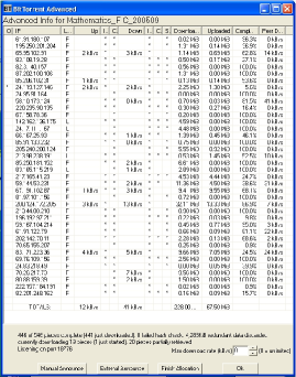
Figure 1: Screenshot of the advanced properties of BitTorrent during a downloading phase.

Figure 1 shows a standard screenshot of the advanced BitTorrent window while downloading a file of size roughly $272Mb$. As it is described in the figure, there are $38$ peers participating in the protocol with $15$ roots and $23$ peers while the number of chunks is $546$ that is $512Kb$ per chunk. It is worth noting that under those circumstances the success of these protocols has to reside in the adopted strategies, in contrast with that outlined in [8]. In such a setting, for instance, the “rarest pieces” distribution becomes quite important. This is the peculiarity in BitTorrent for which once an empty peer appears in the network it is provided with the least common chunk among the network. Also the “altruistic user behavior” is quite crucial from the point of view of the network survivability. It is based on the observable fact for which peers that terminate their download do not immediately disappear. In [2] for instance, it is pointed out how friendly users usually behave in the network. They do not disappear as soon as their download is finished thus ensuring that all the chunks are available. Indeed most of the time this happens since whoever is downloading has just left the computer unattended but working.

1.3 Outline

The remainder of the paper is organized as follows. In the next section we give our first insight of P2P networks by introducing the so called Spreading Scenario. We show under which conditions a file is successfully spread over the network, hence remains alive. Section 3 describes the so called Distributed Scenario. We show under which conditions a file spread over the network can survive according to the number of peers composing the network and the number of chunks in which the file is split. Section 4 is devoted to the so called Survivability Scenario. In this case the behavior of the network is studied under critical circumstances like the high volatility of peers persistence. Section 5 provides a simple model for P2P networks in order to obtain numerical results about peers volatility, chunks distributions and downloading rate. Finally, Section 6 provides some conclusive remarks.

2 Spreading Scenario

In this section we study our first scenario in which a file must be distributed among the network by spreading its $k$ chunks. Our model is synchronous. At round $t$ the network is composed by $R_{t}$ roots that disappear with probability $\alpha_{R}$. In this scenario we do not take into account the number of peers. Usually peers are much more than roots but for our analysis we just consider that a root can provide one chunk to one single peer at each round. This can be seen also by considering at round $t$ a number of peers equal to $R_{t}$ since we are just analyzing the number of rounds needed by the roots in order to spread the file. At a generic round $t$ each peer asks a root for one random chunk. A root answers with a random chunk that has never been spread inside the network before. This implements the previously described “rarest pieces” issue. After each round, roots coordinate with each other in order to maintain the list of chunks that have been sent across the network.

The process is then similar to a coupon collector problem [8]. All the $k$ chunks have to be collected, but a chunk can be collected several times during a round. Moreover the number of roots from which one can collect a coupon decreases exponentially. Let $K_{t}$ be the number of chunks to be collected at time $t$, i.e., chunks that have not been distributed until round $t$.

For a given chunk $x$:

$$Pr(x\mbox{ is not collected})=\left(1-\frac{1}{K_{t}}\right)^{R_{t}}=\left(1-\frac{1}{K_{t}}\right)^{K_{t}\frac{R_{t}}{K_{t}}}\approx e^{-\frac{R_{t}}{K_{t}}}$$

hence $E[K_{t+1}|K_{t}]\approx e^{-\frac{R_{t}}{K_{t}}}K_{t}$. Assuming for now that $K_{t}=E[K_{t}]$ with probability $1$ we get $E[K_{t+1}]\approx e^{-\frac{R_{t}}{K_{t}}}E[K_{t}]$.

For $R_{t}$ the situation is simpler since $R_{t}$ is just the sum of $R$ independent variables, (each one being described by the series $\sum Pr(R_{t+1}=i)z^{i}=(\alpha_{R}+z(1-\alpha_{R}))^{R_{t}}$, and $R_{t}$ is concentrated around its mean $(1-\alpha_{R})R_{t}$. So we have $E[R_{t+1}]=\alpha_{R}E[R_{t}]$.

Let $\rho_{t}=E[R_{t}]/E[K_{t}]$, we get

$$\rho_{t+1}=(1-\alpha_{R})e^{\rho_{t}}\rho_{t}.$$

From this, two situations can follow. If $(1-\alpha_{R})e^{\rho_{0}}\geq 1$, then $\rho_{t}$ always increases, and this increase is faster and faster. This implies that the spreading will easily succeed since the number of chunks not spread decreases much faster than the number of roots that leave the network. Conversely, if $(1-\alpha_{R})e^{\rho_{0}}<1$, $\rho$ decreases and keep doing it faster and faster. This means that the process dies soon.

In the first situation we almost always collect all the chunks otherwise never. Of course, either at some point the chunks are all distributed or there are no roots that can provide the missing chunks. We can conclude from this first analysis that the file gets spread whenever $\alpha_{R}<1-e^{-\frac{R}{k}}$. Note that when $k>>R$ this actually means $\alpha_{R}<\frac{R}{k}$ and this is usually the case. For $k=R$ we get $\alpha_{R}\leq\frac{e-1}{e}$ but, in real world scenarios, this usually does not happen.

3 Distributed Scenario

In the previous section we gave a necessary and sufficient condition to describe the asymptotic behavior of the network. That is, the network must move from the initial state to the distributed state. In this section we study the behavior of P2P networks in the distributed state, that is, there are no roots, yet every chunk is available on the network after time $t$. In the following we refer to [10] for the applied probabilistic tools.

3.1 Upper bound

Our next goal is to show that networks that are in the distributed state will not survive if the number of chunks is exponentially big in the number of peers. In order to show this we assume the following model. In each time step each peer asks a random chunk among all the chunks that the peer is missing. We assume that if the chunk is anywhere on the network then the peer will get this chunk in the next time step. Clearly this assumption is optimistic and will help the survival of the network. Importantly, this makes the network’s gross behavior deterministic and thus we can say with certainty that every peer stays precisely $k$ timesteps before leaving, since he gets exactly $1$ chunk per timestep. When a new peer enters, it has no chunks and we may use the variable $i$, with $0\leq i<n$, to indicate its ordering when all peers are sorted according to their number of chunks. This ordering is equivalent to the chronological ordering. After $\frac{k}{n}$ time steps, each peer is promoted to the next ordinal position. We point out that nothing changes in the network viability unless a peer leaves, and further the only peer that may leave is the last one, or the one with the most chunks; eventually the last peer will have $k$ chunks when the file has been completely downloaded. We wish to bound the probability that a chunk will be missing. Therefore the number of chunks that each peer $i$ has is $\frac{k(i-1)}{n}$ whenever a peer is leaving.

To be precise, we imagine the total network state at any time to be given by a binary vector of length $kn$; that is,

$$\Omega=\left(\{0,1\}^{k}\right)^{n}.$$

In $\Omega$, the first $k$ coordinates describe the chunks held by the first peer. In this first part, the first coordinate is $1$ if and only if the first peer holds the first chunk, otherwise, it is $0$. The next coordinate indicates the next chunk, and so on for all $k$ chunks.

We will define an event $G$ on $\Omega$ such that $\forall i=1..n$, peer $i$ has exactly $\frac{ik}{n}$ chunks. Let $A^{j}_{i}$ be the event that peer $i$ has chunk $j$. Let $X^{j}_{i}$ be the indicator variable of $A^{j}_{i}$. Let $Y^{j}=\max\{X^{j}_{1},X^{j}_{2}...,X^{j}_{n}\}$, i.e., $Y^{j}$ is the indicator variable of the event that chunk $j$ is in the system. We define the random variable $Z=\min\{Y^{1},...,Y^{k}\}$ as follows: it is the indicator variable of the event that there is a missing chunk in the network. In other words, $Z=0$ means the network has died, and $Z>0$ means it continues to distribute the file.

Lemma 1

Let $n$ and $k$ be the number of peers and chunks in the system respectively. For $n>2$, the probability that there is a missing chunk can be bounded by $\Pr[Z=0]\leq kne^{-n}$.

Proof

by the Union bound over all $k$ chunks,

$$\Pr[Z=0]<k\Pr[Y^{1}=0]=k\prod_{i=1}^{n}\frac{i}{n}=k\frac{n!}{n^{n}}$$

and by Sterling’s approximation,

$$k\frac{n!}{n^{n}}<kne^{-n}.$$

$\hfill\square$

The next corollary shows that if the number of chunks is small the probability for the network to die approaches 0.

Corollary 1

For all $k<\frac{e^{n}}{n\log n}$,

$$\lim_{n\rightarrow\infty}\Pr[Z=0]=0.$$

The next corollary shows that if the number of chunks is small the system survives for a long time.

Corollary 2

If the number of chunks is a polynomial ${\rm Poly}(n)$ then the expected survival time is at least $\frac{e^{n}}{n{\rm Poly}(n)}.$

3.2 Lower bound

The main problem in proving the lower bound is the dependence between the random variables $Y^{j}$ and $Y^{j^{\prime}}$. To remove this technical difficulty we use a different model, the binomial model. The idea is to make $Y^{j}$ and $Y^{j^{\prime}}$ i.i.d. variables. In order to prove a lower bound on the previous model we increase the expected number of chunks that peer $i$ has at the time the last peer leaves the network. I.e., we relax the assumption that, at the time the last peer leaves the network, the number of chunks in the peer $i$ is $\frac{k(i-1)}{n}$. Moreover we assume that the number of chunks is a binomial random variable. This assumption is legitimate since the binomial distribution is highly concentrated. The problem with this approach is that now we are no longer sure that each peer has enough chunks. The way we solve this problem is by strengthening the peer capabilities by increasing the chance that a peer has received chunk $i$. Since in a normal file sharing system chunks are correlated and peers have a smaller number of chunks, our lower bound also captures the behavior of these systems. This is justified since both assumptions (increasing the number of packets and the fact that packets are i.i.d) decrease the probability of failure. We do not offer a method to achieve this, but rather we use this approach to prove a lower bound with high probability. We posit this property (the binomial distribution) for the proof. We assume that the peers $i=1,...,n$ have $\frac{ki}{n+1}$ chunks on average. More precisely, let $\mathcal{X}^{j}_{i}$ be a Bernoulli random variable such that $E[\mathcal{X}^{j}_{i}]=\frac{i}{n+1}$. Let $\mathcal{G}_{i}=\sum_{j=1}^{k}\mathcal{X}^{j}_{i}$ be a random variable that counts the number of chunks that peer $i$ has. Note that $E[\mathcal{G}_{i}]=\frac{ki}{n+1}$. The next lemma bounds the probability that peer $i$ will have less than $\frac{(i-1)k}{n}$ chunks.

Lemma 2

Let $\mathcal{G}_{i}$ be the number of different chunks belonging to peer $i$. For all $1\leq i\leq n$, $\Pr[\mathcal{G}_{i}<\frac{(i-1)k}{n}]<e^{-\frac{k}{2n^{3}(n+1)}}$.

Proof

$$\Pr\left[\mathcal{G}_{i}<\frac{k(i-1)}{n}\right]=\Pr\left[\mathcal{G}_{i}<\left(1-\frac{n+1-1}{in}\right)\frac{ki}{(n+1)}\right]<$$

$$<e^{-\big{(}\frac{n+1-i}{in}\big{)}^{2}\frac{ki}{2(n+1)}}<e^{-\frac{k}{{2n^{3}(n+1)}}}$$

The first equality follows from algebra, and a Chernoff bound yields the next inequality. $\hfill\square$

If $k>>n^{4}$ we get that the probability that the $i$-peer (Bernoulli process) has less than $\frac{(i-1)k}{n}$ chunks is exponentially small.

Let $Q=\bigcap_{i=0}^{n-1}\{\mathcal{G}_{i}\geq\frac{(i-1)k}{n}\}$. Note that $Q$ is the event that all peers have more chunks than they are supposed to have, i.e., for all $i$, $\mathcal{G}_{i}\geq\frac{(i-1)k}{n}$.

Lemma 3

For all $\log k>n$, $\Pr[Q]>1-ne^{-\frac{k}{2(n+1)n^{3}}}$.

Proof

$$\Pr[Q]=\prod_{i=1}^{n}\Pr\left[\mathcal{G}_{i}\geq\frac{k(i-1)}{n}\right]=$$

$$=\prod_{i=1}^{n}\left(1-\Pr\left[\mathcal{G}_{i}<\frac{k(i-1)}{n}\right]\right)\geq\prod_{i=1}^{n}\left(1-e^{-\frac{k}{2(n+1)n^{3}}}\right).$$

We apply Lemma 2 to derive the last inequality above. We choose the smallest term in the product and raise it to the $n$ power for the bound:

$$\Pr[Q]\geq\left(1-e^{-\frac{k}{2(n+1)n^{3}}}\right)^{n}>1-ne^{-\frac{k}{2(n+1)n^{3}}}.$$

$\hfill\square$

Using the previous lemma it follows that the probability for which $\overline{Q}$ holds is exponentially small.

Corollary 3

For all $\log k>n$, $\Pr[\overline{Q}]<ne^{-\frac{k}{2(n+1)n^{3}}}$.

After bounding the probability that all the Bernoulli peers will have more chunks than the discrete peers, we analyze the probability that the Bernoulli peers will fail, i.e., some chunk is missing. Let $\mathcal{Y}^{j}=\max\{\mathcal{X}^{j}_{1},\mathcal{X}^{j}_{2}...,\mathcal{X}^{j}_{n}\}$, $\mathcal{Z}=\min\{\mathcal{Y}^{1},...,\mathcal{Y}^{k}\}$. Note that $\mathcal{Z}=0$ is equivalent to say that the Bernoulli peers will fail.

The following lemmata lead to the last corollary that shows under which condition the network goes to miss some chunk, i.e., it is not able to deliver any further complete download.

Lemma 4

The probability that the Bernoulli peers will fail is,

$$\Pr[\mathcal{Y}^{j}=0]>\frac{1}{e^{n+1}}.$$

Proof

The proof follows from the following computation.

$$\Pr[\mathcal{Y}^{j}=0]=\prod_{i=1}^{n}\frac{i+1}{n+1}=\frac{(n+1)!}{(n+1)^{n}}>\frac{\frac{(n+1)^{n+1}}{e^{n+1}}}{(n+1)^{n+1}}=\frac{1}{e^{n+1}}.$$

$\hfill\square$

Lemma 5

$$\Pr[\mathcal{Z}>0]<e^{-\frac{k(n+1)}{e^{n+1}}}.$$

Proof

In order to prove the claim we make use of Lemma 4, followed by the limit definition of $e$ and then Sterling’s approximation, hence obtaining

$$\Pr[\mathcal{Z}>0]=\prod_{j=1}^{k}\left(1-\Pr[\mathcal{Y}^{j}=0]\right)=\left(1-\frac{(n+1)!}{(n+1)^{n}}\right)^{k}\cong e^{-\frac{k(n+1)!}{(n+1)^{n}}}<e^{-\frac{k(n+1)}{e^{n+1}}}.$$

$\hfill\square$

Lemma 6

For $\log k>n$,

$$\Pr[Z=0]\geq 1-e^{-\frac{k(n+1)}{e^{n+1}}}-ne^{-\frac{k}{2(n+1)n^{3}}}.$$

Proof

From Bayes Law and the complementary events property,

$$\Pr[Z=0]>\Pr[\mathcal{Z}=0|Q]=\Pr[\mathcal{Z}=0]-\Pr[\overline{Q}]\Pr[\mathcal{Z}=0|\overline{Q}]>$$

$$>\Pr[\mathcal{Z}=0]-\Pr[\overline{Q}]\geq 1-e^{-\frac{k(n+1)}{e^{n+1}}}-ne^{-\frac{k}{2(n+1)n^{3}}}.$$

$\hfill\square$

Corollary 4

For all $k\geq\frac{\log n}{n+1}e^{n+1}$,

$$\lim_{n\rightarrow\infty}\Pr[Z=0]=1.$$

From the previous corollary it follows that if the number of chunks $k$ is bigger than or equal to $\frac{\log n}{n+1}e^{n+1}$, then the expected survival time is constant.

4 Survivability Scenario

In this section we study how likely the network is to survive in extreme conditions. With extreme conditions we mean that a file is almost never downloaded since peers have a very high volatility and almost never stay in the network long enough to perform a full download. However, it is still very interesting to note that the network is able to survive. We remind that a network survives whenever it still contains all the $k$ chunks composing the original file, no matter where they reside. We will assume that peers leave the system with probability $\alpha$ while roots or experts (peers that succeed at the full download) leave the network with probability $\alpha_{R}$.

During the process chunks are duplicated and hence created while others disappear because of nodes leaving the system. Let us denote by $N$ the number of nodes (peers plus experts, assuming roots as experts) in the network and by $P_{i}$ the probability (percentage of peers) that a peer has $i$ chunks. The number of chunks lost during one time step is then:

$$N\left(\alpha\sum_{i=0}^{k-1}iP_{i}+\alpha_{R}P_{k}\right).$$

The amount $C$ of chunks created, depends on how many successful download are performed during a step. This strongly depends on the chosen protocol. In any case this amount cannot be more than the number of peers with one packet $N(1-P_{0})$ multiplied by the probability to stay inside the network, i.e., $C\leq(1-\alpha)N(1-P_{0})$.

Hence a necessary condition for the network survival is that

$$N(1-P_{0})(1-\alpha)\geq N\left(\alpha\sum_{i=0}{k-1}iP_{i}+\alpha_{e}P_{k}\right)\geq N\alpha(1-P_{0})$$

and this leads to have $1-\alpha\geq\alpha$, i.e., $\alpha\leq\frac{1}{2}$.

When $\alpha=\frac{1}{2}$ the stationary distribution is as follows $P_{0}=P_{1}=\frac{1}{2}$, after each communication step all the nodes have a chunk, but then half of them die (reset to zero chunks). Note that such a network dies quite quickly, from deviations. However, as soon as $\alpha>\frac{1}{2}$ the network lives almost forever.

Our process is very similar to a birth and death process, each node lives on average $\frac{1}{1-\alpha}$ rounds. And at each round it generates $1-\alpha$ chunks, hence its average number of children is $\frac{1-\alpha}{\alpha}$. It holds that when this number is strictly greater than $1$ the network survives.

Let us assume the network to be in some random state with $P_{0}=P_{1}=\frac{1}{2}$, with $k$ chunks regularly spread across the peers with one chunk each. Let $F_{i,t}$ be a random variable that denotes the percentage of peers with the $i$-th chunk at time $t$. $F_{i,0}$ is deterministic with value $\frac{N}{2k}$.

After the first step of the protocol, we have:

$$P[F_{i,1}=k]={2F_{0,t}\choose k}/2^{2F_{i,0}}$$

So after the initial step, chunks are distributed as the sum of $\frac{N}{2k}$ random bits.

We study this phenomenon at the critical point in its most canonical form. At time $t$ we have a number $S_{t}$ of chunks alive, we double each chunk and randomly destroy half of the chunks.

First we consider the future of a single chunk. Let $F_{t}(z)$ denote the generating series at time $t$ associated with the future of chunk $z$.

Considering one time step we have: with probability $\frac{1}{4}$ the process dies, with probability $\frac{1}{2}$ the process restarts with $1$ chunk and $t-1$ time units remain, with probability $\frac{1}{4}$ we get two chunks and $t-1$ time units remain.

$$F_{t}(z)=\frac{1}{4}+\frac{1}{2}F_{t-1}(z)+\frac{1}{4}F^{2}_{t-1}(z)=\left(\frac{F_{t-1}(z)+1}{2}\right)^{2}$$

Note that by setting $\varepsilon_{t}(z)_{t}=F_{t}(z)-1$, we obtain

$$\varepsilon_{t}(z)=\varepsilon_{t-1}(z)+\left(\frac{\varepsilon_{t-1}(z)}{2}\right)^{2}$$

and $\varepsilon_{t}(0)$ is the probability to stop before time $t$. So the probability to have the process alive at time $t$ is about $\frac{t}{\ln t}$, and if one considers $n$ bits one needs $n\ln n$ time units to kill all of them.

This scenario is quite optimistic since one assumes that the network exchanges $N(1-P_{0})$ chunks during a round which corresponds to a perfect situation. This happens, in fact, by means of a perfect matching between the nodes that meet their necessities. Indeed, if we make use of a non optimal strategy, i.e., matching the node in a perfectly arbitrarily way, it is worth noting that this does not affect and degrade the process too much.

A typical way to marry the nodes is to choose randomly for each node a server, and to elect a node randomly for each server. Despite the simplicity of this process (nodes which have all the chunks still demand some, and nodes with no chunks are considered as able to provide some), it does not affect the network survivability as we are going to see.

Note that, by means of a simple matching algorithm, the number of edges is already of order $(1-\frac{1}{e})N$. Among those edges some are unable to duplicate chunks (if the server does not have any chunks that the client needs). A critical stage occurs when almost all the nodes with chunks have almost no chunks, so the probability for an edge to be useful is indeed exactly $(1-P_{0})$. In such a situation the number of chunks replicated is

$$\left(1-\frac{1}{e}\right)\left(1-P_{0}\right)\left(1-\alpha\right)$$

while the number of chunks destroyed is at least $\alpha(1-P_{0})$. This implies that the network survives when $\alpha\leq\frac{1-\frac{1}{e}}{2-\frac{1}{e}}\simeq.3873$.

5 Simple evaluation Model for P2P Networks

To better understand the behavior of this kind of network we propose a simplified model and protocol. Such a model can be easily applied and modified in order to find preliminary results on P2P networks. We have also compared our easy model’s results to the outputs of more sophisticated simulators. Even though the comparison is outside the scope of this paper, it is worth mentioning that the deviation from the simulations is negligible.

• At the beginning of each time slot, each peer chooses another peer randomly. An inquired peer randomly selects one of its customers. We call this customer lucky. Next the uploading peer delivers to its lucky customer a useful random chunk, i.e., a chunk that he has and that this customer has not. The unlucky customers do not get any chunk at this round.
  

• In order to get a stable situation, each peer that disappears (with probability $\alpha$) is immediately replaced by a new empty peer (i.e., with no chunks).

The probability $luck$ that a customer gets lucky is indeed equal to the proportion of customers served, which is the number of peers having at least one customer. Hence, $luck=1-\frac{1}{e}$.

We first compute the probability that a node with $i$ chunks gets a new useful one. To do this we make a strong assumption that chunks remains almost identically distributed, i.e., a random node with $i$ chunks contains a given chunk with probability $\frac{i}{k}$.

To get a chunk, a node needs first to be lucky, then the probability that it gets a chunk depends on the number of chunks of its uploading peer. Assume that a customer with $i$ chunks contacts an uploading peer with $j$ chunks, its probability to receive a chunk is

$$\Delta_{i,j}=1-\frac{{i\choose j}}{{k\choose j}}$$

Note that we use the standard convention ${i\choose j}=0$ whenever $j\geq i$, but in the case $i=j=0$ we have $\Delta_{i,j}=0$, so we consider ${0\choose 0}=1$. It follows that a lucky node in state $i$ that does not vanish (i.e., conditioned on all those events) moves to states $i+1$ with probability

$$\sum_{j=0*}^{k}\Delta_{ij}P_{j}$$

From that it follows that a peer in state $i\neq 0$ moves to:

• State $i+1$ with probability $T_{i,i+1}=(1-\alpha)luck\sum_{j=0}^{k}\Delta_{i,j}P_{j}$

• State $i$ with probability $T_{i,i}=(1-\alpha)-T_{i,i+1}$

• State $0$ with probability $\alpha$

To summarize we have:

$$P_{0}=\alpha\sum_{i=0}^{k}P_{j}+\left(1-\alpha\right)\left(1-luck\sum_{j=0}^{k}\Delta_{0,j}P_{j}\right),$$

$\forall i>0,$

$$P_{i}=(1-\alpha)\left(P_{i}\left(1-luck\sum_{j=0}^{k}\Delta_{i,j}P_{j}\right)+P_{i-1}\left(luck\sum_{j=0}^{k}\Delta_{i-1,j}P_{j}\right)\right).$$

For the aim of preliminary and experimental results such a model is already enough in order to get an idea of the general behavior of this class of networks.

6 Conclusion

In this paper we have studied the behavior of P2P networks. We have considered three main scenarios. In the first one there are some peers owning all the chunks (roots) composing a file and the aim is to study the time required to ensure that every chunk is spread out on the network. This is very important to understand since, of course, it reflects the required behavior for peers that want to share their information. We have shown that the success of the spreading phase depends on two main parameters. Namely, the number of roots in the network and the number of chunks in which the file is divided. The probability $\alpha_{R}$ for which $R$ roots can leave the network should be smaller than $1-e^{-\frac{R}{k}}$ where $k$ is the number of chunks. In the second scenario, we have started with a configuration in which many peers have subsets of the whole chunk set and the aim is to study the probability for the network to survive, i.e., every chunk must belong to some peer. This is also very important since it gives a measure of the behavior that peers should exhibit in order to maintain the viability of their download and archival capabilities. We have shown that if $k$ is much less than $e^{n}$, with $n$ being the number of peers in the network, the expected survival time of the network is exponential in $n$. Moreover, if the number of chunks is greater than $\frac{\log n}{n+1}e^{n}+1$, the network survival time is constant. The third proposed scenario concerns the critical setting for the peers in terms of volatility. We have shown how under this setting the network is still able to survive. Namely, our estimated maximum value of the probability $\alpha$ for which a peer can leave the network while guaranteing its survivability is $\alpha\leq.3873$. From the point of view of experimental results, we have also proposed a simple way for analyzing and modeling P2P networks.

Our study has raised many open questions that might be investigated for further research. Many variations of our proposed models are possible and interesting. An important issue, for instance, concerns file sharing protocols that cope with security aspects. Deep analysis of tit-for-tat strategies for avoiding the so called free-riders problem is of primary interest to better understand the success of these protocols (see [11] for preliminary results). Free-riders are users that download files from the network but do not share their own chunks. In BitTorrent, those kind of users are allowed even though the performance of their downloads is much slower than for “friendly” users.

References

- [1] Sun, T., Tamai, M., Yasumoto, K., Shibata, N., Ito, M., Mori, M.: MTcast: Robust and Efficient P2P-based Video Delivery for Heterogeneous Requirements. In: Proceedings of the 9th International Conference on Principles of Distributed Systems (OPODIS). Lecture Notes in Computer Science, Springer-Verlag (2005)
- [2] Izal, M., Urvoy-Keller, G., Biersack1, E.W., Felber, P., Hamra, A.A., Garces-Erice, L.: Dissecting BitTorrent: Five Months in a Torrent’s Lifetime. In: Proceedings of the 5th International Workshop on Passive and Active Network Measurement (PAM). Volume 3015 of Lecture Notes in Computer Science., Springer-Verlag (2004) 1–11
- [3] Cohen, B.: Incentives Build Robustness in BitTorrent. In: Proceedings of the 1st Workshop on the Economics of Peer-to-Peer Systems (Econ P2P). (2003)
- [4] Clevenot, F., Nain, P.: A Simple Fluid Model for the Analysis of the Squirrel Peer-to-Peer Caching System. In: Proceedings of the 23rd Annual Joint Conference of the IEEE Computer and Communications Societies (INFOCOM), IEEE Computer Society (2004)
- [5] Qiu, D., Srikant, R.: Modeling and performance analysis of bittorrent-like peer-to-peer networks. In: Proceedings of Conference on Applications, technologies, architectures, and protocols for computer communications (SIGCOMM), ACM Press (2004) 367–378
- [6] Ge, Z., Figueiredo, D.R., Jaiswal, S., Kurose, J., Towsley, D.: Modeling peer-peer file sharing systems. In: Proceedings of the 22nd Annual Joint Conference of the IEEE Computer and Communications Societies (INFOCOM), IEEE Computer Society (2003)
- [7] Jain, K., Lovasz, L., Chou, P.A.: Building scalable and robust peer-to-peer overlay networks for broadcasting using network coding. In: Proceedings of the 24th annual ACM SIGACT-SIGOPS symposium on Principles of distributed computing (PODC), ACM Press (2005) 51–59
- [8] Massouli, L., Vojnovi, M.: Coupon replication systems. ACM SIGMETRICS Performance Evaluation Review 33(1) (2005) 2–13
- [9] Arthur, D., Panigrahy, R.: Analyzing bittorrent and related peer-to-peer networks. In: Proceedings of the 17th annual ACM-SIAM symposium on Discrete algorithm (SODA), ACM Press (2006) 961–969
- [10] Williams, D.: Probability with Martingales. Cambridge University Press (1991)
- [11] Jun, S., Ahamad, M.: Incentives in bittorrent induce free riding. In: Proceeding of the 3rd Workshop on Economics of Peer-to-Peer Systems (Econ P2P), ACM Press (2005) 116–121