Zig-zag and Replacement Product Graphs and LDPC Codes

Abstract.

The performance of codes defined from graphs depends on the expansion property of the underlying graph in a crucial way. Graph products, such as the zig-zag product [13] and replacement product provide new infinite families of constant degree expander graphs. The paper investigates the use of zig-zag and replacement product graphs for the construction of codes on graphs [16]. A modification of the zig-zag product is also introduced, which can operate on two unbalanced biregular bipartite graphs.

Christine A. Kelley Deepak Sridhara Joachim Rosenthal The Ohio State University 1251 Waterfront Place Institut f$\ddot{\mbox{u}}$r Mathematik Department of Mathematics Seagate Technology Universit$\ddot{\mbox{a}}$t Z$\ddot{\mbox{u}}$rich Columbus, OH 43210 Pittsburgh, PA 15222 CH-8057, Switzerland. ckelley@math.ohio-state.edu deepak.sridhara@seagate.com rosen@math.unizh.ch

(Communicated by Aim Sciences)

1. Introduction

Expander graphs are of fundamental interest in mathematics and engineering and have several applications in computer science, complexity theory, designing communication networks, and coding theory [8, 1, 17]. In a remarkable paper [13] Reingold, Vadhan, and Wigderson introduced an iterative construction which leads to infinite families of constant degree expander graphs. The iterative construction is based on the zig-zag graph product introduced by the authors in the same paper. The zig-zag product of two regular graphs is a new graph whose degree is equal to the square of the degree of the second graph and whose expansion property depends on the expansion properties of the two component graphs. In particular, if both component graphs are good expanders, then their zig-zag product is a good expander as well. Similar things can be said about the replacement product.

Since the work of Sipser and Spielman [15] it has been well known that the performance of codes defined on graphs depends on the expansion property of the underlying graph in a crucial way. Several authors have provided constructions of codes from graphs whose underlying graphs are good expanders. In general, a graph that is a good expander is particularly suited for the message-passing decoder that is used to decode low density parity check (LDPC) codes, in that it allows for messages to be dispersed to all nodes in the graph as quickly as possible. Furthermore, graphs with good expansion yield LDPC codes with good minimum distance and pseudocodeword weights [4, 6, 7, 14, 15].

Probably the most prominent example of expander graphs are the class of Ramanujan graphs which are characterized by the property that the second eigenvalue of the adjacency matrix is minimal inside the class of $k$-regular graphs on $n$ vertices. This family of ‘maximal expander graphs’ was independently constructed by Lubotzky, Phillips and Sarnak [10] and by Margulis [11]. The description of these graphs and their analysis rely on deep results from mathematics using tools from graph theory, number theory, and representation theory of groups [9]. Codes from Ramanujan graphs were constructed and studied by several authors [7, 14, 18].

Ramanujan graphs have the drawback that they exist only for a limited set of parameters. In contrast, the zig-zag product and the replacement product can be performed on a large variety of component graphs. The iterative construction also has a lot of engineering appeal as it allows one to construct larger graphs from smaller graphs as one desires. This was the starting point of our research reported in [5].

In this paper we examine the expansion properties of the zig-zag product and the replacement product in relation to the design of LDPC codes. We also introduce variants of the zig-zag scheme that allow for the component graphs to be unbalanced bipartite graphs. In our code construction, the vertices of the product graph are interpreted as sub-code constraints of a suitable linear block code and the edges are interpreted as the code bits of the LDPC code, as originally suggested by Tanner in [16]. Codes obtained in this way will be referred to as generalized LDPC (GLDPC) codes. By choosing component graphs with relatively small degree, we obtain product graphs that are relatively sparse. Examples of each product and resulting LDPC codes are given to illustrate the results of this paper. Some of the examples use Cayley graphs as components, and the resulting product graph is also a Cayley graph with the underlying group being the semi-direct product of the component groups, and the new generating set being a function of the generating sets of the components [2]. Simulation results reveal that LDPC codes based on zig-zag and replacement product graphs perform comparably to, if not better than, random LDPC codes of comparable block lengths and rate. The vertices of the product graph must be fortified with strong (i.e., good minimum distance) sub-code constraints, in order to achieve good performance with message-passing (or, iterative) decoding.

The paper is organized as follows. Section 2 discusses preliminaries on the formal definition of expansion for a $d$-regular graph and the best one can achieve in terms of expansion. Furthermore, expansion for a general graph is discussed. Section 3 describes the original zig-zag product and replacement product. A first result on the girth and diameter of the replacement product is derived.

Section 4 contains a new zig-zag product construction of unbalanced bipartite graphs. The main result is Theorem 1 which essentially states that the constructed bipartite graph is a good expander graph if the two component graphs are good expanders.

Section 5 is concerned with applications to coding theory. The section contains several code constructions using the original and the unbalanced bipartite zig-zag products and the replacement product. Simulation results of the LDPC codes constructed in Section 5 are presented in Section 6. Section 7 introduces a new iterative construction for an unbalanced bipartite zig-zag product and the replacement product to generate families of expanders with constant degree. For completion, the iterative construction for the original zig-zag product from [13] is also described. The expansion for the iterative families are also discussed. Section 8 summarizes the results and concludes the paper.

2. Preliminaries

In this section, we review the basic graph theory notions used in this paper.

Let $G=(V,E)$ be a graph with vertex set $V$ and edge set $E$. The number of edges involved in a path or cycle in $G$ is called the length of the path or cycle. The girth of $G$ is the length of the shortest cycle in $G$. If $x,y\in V$ are two vertices in $G$, then the distance from $x$ to $y$ is defined to be the length of the shortest path from $x$ to $y$. If no such path exists from $x$ to $y$, then we say the distance from $x$ to $y$ is infinity. The diameter of $G$ is the maximum distance among all pairs of vertices of $G$.

Intuitively, a graph has good expansion if any small enough set of vertices in the graph has a large enough set of vertices connected to it. It is now almost common knowledge that for a graph to be a good expander [15], the second largest eigenvalue of the adjacency matrix $A$ must be as small as possible compared to the largest eigenvalue [17]. For a $d$-regular graph $G$, the index (or, the largest eigenvalue) of the adjacency matrix $A$ is $d$. Hence, by normalizing the entries of $A$ by the factor $d$, the normalized matrix $\tilde{A}=\frac{1}{d}A$ has the largest eigenvalue equal to $1$.

Definition 1.

Let $G$ be a $d$-regular graph on $N$ vertices. Denote by $\lambda(G)$ the second largest eigenvalue of the normalized adjacency matrix $\tilde{A}$ representing $G$. $G$ is said to be a $(N,d,\lambda)$-graph if $\lambda=\lambda(G)$.

In this paper, we will follow the definition provided in [2, 12] for a graph to be an expander.

Definition 2.

A sequence of graphs is said to be an expander family if for every (connected) graph $G$ in the family, the second largest eigenvalue $\lambda(G)$ is bounded below some constant $\kappa<1$. In other words, there is an $\epsilon>0$ such that for every graph $G$ in the family, $\lambda(G)<1-\epsilon$. A graph belonging to an expander family is called an expander graph.

Alon and Boppana have shown that for a $d$-regular graph $G$, as the number of vertices $n$ in $G$ tends to infinity, $\lambda(G)\geq\frac{2\sqrt{d-1}}{d}$ [1]. For $d$-regular (connected) graphs, the best possible expansion based on the eigenvalue bound is achieved by Ramanujan graphs that have $\lambda(G)\leq\frac{2\sqrt{d-1}}{d}$ [10]. Hence, Ramanujan graphs are optimal in terms of the eigenvalue gap $1-\lambda(G)$.

The definition of expansion to $d$-regular graphs can be similarly extended to $(c,d)$-regular bipartite graphs as defined below and also to general irregular graphs.

Definition 3.

A graph $G=(X,Y;E)$ is $(c,d)$-regular bipartite if the set of vertices in $G$ can be partitioned into two disjoint sets $X$ and $Y$ such that all vertices in $X$ (called left vertices) have degree $c$ and all vertices in $Y$ (called right vertices) have degree $d$ and each edge $e\in E$ of $G$ is incident with one vertex in $X$ and one vertex in $Y$, i.e., $e=(x,y),x\in X,y\in Y$.

Definition 4.

A $(c,d)$-regular bipartite graph $G$ on $N$ left vertices and $M$ right vertices is said to be a $(N,M,c,d,\lambda)$-graph if the second largest eigenvalue of the normalized adjacency matrix $\tilde{A}$ representing $G$ is $\lambda$.

The largest eigenvalue of a $(c,d)$-regular graph is $\sqrt{cd}$. Once again, normalizing the adjacency matrix of a $(c,d)$-regular bipartite graph by its largest eigenvalue $\sqrt{cd}$, we have that the (connected) graph is a good expander if second largest eigenvalue of its normalized adjacency matrix is bounded away from 1 and is as small as possible.

To normalize the entries of an irregular graph $G$ defined by the adjacency matrix $A=(a_{ij})$, we scale each $(i,j)^{th}$ entry in $A$ by $\frac{1}{r_{i}c_{j}}$, where $r_{i}$ and $c_{j}$ are the $i^{th}$ row weight and $j^{th}$ column weight, respectively, in $A$. It is easy to show that the resulting normalized adjacency matrix has its largest eigenvalue equal to one. The definition of an expander for an irregular graph $G$ can be defined analogously.

3. Graph Products

In designing codes over graphs, graphs with good expansion, relatively small degree, small diameter, and large girth are desired. Product graphs give a nice avenue for code construction, in that taking the product of small graphs suitable for coding can yield larger graphs (and therefore, codes) that preserve these desired properties. Standard graph products, however, such as the Cartesian product, tensor product, lexicographic product, and strong product, all yield graphs with large degrees. Although sparsity is not as essential for generalized LDPC codes, large degrees significantly increase the complexity of the decoder.

In this section we describe the zig-zag product of [8, 13], introduce a variation of the zig-zag product that holds for bi-regular (unbalanced) bipartite graphs, and review the replacement product. In each case, the expansion of the product graph with respect to the expansion of the component graphs is examined. When the graph is regular-bipartite, this bi-regular product yields the product in [8, 13]. In addition to preserving expansion, these products are notable in that the resulting product graphs have degrees dependent on only one of the component graphs, and therefore can be chosen to yield graphs suitable for coding.

3.1. Zig-zag product

Let $G_{1}$ be a $(N_{1},d_{1},\lambda^{(1)})$-graph and let $G_{2}$ be a $(d_{1},d_{2},$ $\lambda^{(2)})$-graph. Randomly number the edges around each vertex of $G_{1}$ by $\{1,\ldots,d_{1}\}$, and each vertex of $G_{2}$ by $\{1,\ldots,d_{1}\}$.Then the zig-zag product $G=G_{1}\mbox{\scriptsize$Z$⃝}G_{2}$ of $G_{1}$ and $G_{2}$, as introduced in [8, 13], is a $(N_{1}\cdot d_{1},d_{2}^{2},\lambda)$-graph defined as follows:

• vertices of $G$ are represented as ordered pairs $(v,k)$, where $v\in\{1,2,\ldots,N_{1}\}$ and $k\in\{1,2,\dots,d_{1}\}$. That is, every vertex in $G_{1}$ is replaced by a cloud of vertices of $G_{2}$.

• edges of $G$ are formed by making two steps on the small graph and one step on the big graph as follows:

  • a step “zig” on the small graph $G_{2}$ is made from vertex $(v,k)$ to vertex $(v,k[i])$, where $k[i]$ denotes the $i^{th}$ neighbor of $k$ in $G_{2}$, for $i\in\{1,2,\dots,d_{2}\}$.

  • a deterministic step on the large graph $G_{1}$ is made from vertex $(v,k[i])$ to vertex $(v[k[i]],\ell)$, where $v[k[i]]$ is the $k[i]^{th}$ neighbor of $v$ in $G_{1}$ and correspondingly, $v$ is the $\ell^{th}$ neighbor of $v[k[i]]$ in $G_{1}$.

  • a final step “zag” on the small graph $G_{2}$ is made from vertex $(v[k[i]],\ell)$ to vertex $(v[k[i]],\ell[j])$, where $\ell[j]$ is the $j^{th}$ neighbor of $\ell$ in $G_{2}$, for $j\in\{1,2,\dots,d_{2}\}$.

  Therefore, there is an edge between vertices $(v,k)$ and $(v[k[i]],\ell[j])$ for $i,j\in\{1,\dots,d_{2}\}$.

Figure 1. Zig-Zag product of two graphs.

Example 1.

Consider the zig-zag product graph $G=G_{1}\mbox{\scriptsize$Z$⃝}G_{2}$ depicted in Figure 1. The edge from $(1,3)$ (“cloud $a_{1}$, vertex 3”) to $(5,2)$ (“cloud $a_{5}$, vertex 2”) is obtained by the following 3 steps:

$$(1,3)\rightarrow(1,4)\rightarrow(5,3)\rightarrow(5,2)$$

The first step from 3 to 4 in cloud $a_{1}$ takes $(1,3)$ to $(1,4)$. The second step from $a_{1}$ to $a_{5}$ in $G_{1}$ takes $(1,4)$ to $(5,3)$, since $a_{5}$ is the $4$th neighbor of $a_{1}$ and $a_{1}$ is the $3$rd neighbor of $a_{5}$ in the labeling around the vertices of $G_{1}$. The final step in cloud $a_{5}$ takes $(5,3)$ to $(5,2)$. Similarly, vertex $(1,3)$ also connects to $(5,4)$,$(3,4)$, and $(3,6)$ by these steps:

$$(1,3)\rightarrow(1,4)\rightarrow(5,3)\rightarrow(5,4)$$

$$(1,3)\rightarrow(1,2)\rightarrow(3,5)\rightarrow(3,4)$$

$$(1,3)\rightarrow(1,2)\rightarrow(3,5)\rightarrow(3,6),$$

so the degree of vertex $(1,3)$ is $2^{2}=4$ as expected.

It is shown in [13] that the zig-zag product graph $G=G_{1}\mbox{\scriptsize$Z$⃝}G_{2}$ is a $(N_{1}\cdot d_{1},d_{2}^{2},\lambda)$-graph with $\lambda<\lambda^{(1)}+\lambda^{(2)}+[\lambda^{(2)}]^{2}$, and further, that $\lambda<1$ if $\lambda^{(1)}<1$ and $\lambda^{(2)}<1$. Therefore, the degree of the zig-zag product graph depends only on the smaller component graph whereas the expansion property depends on the expansion of both the component graphs, i.e., it is a good expander if the two component graphs are good expanders.

Lemma 1.

Let $G_{1}$ and $G_{2}$ have girth $g_{1}$ and $g_{2}$, respectively. Then the zig-zag product graph $G=G_{1}\mbox{\scriptsize$Z$⃝}G_{2}$ has girth $g=4$.

Proof.

We show that any pair of vertices at distance two in $G_{2}$ are involved in a 4-cycle in $G$. Consider two vertices $(v_{1},k_{1})$ and $(v_{1},k_{2})$ in the same cloud of $G$ that lie at distance two apart in $G_{2}$. Let $(v_{1},k_{3})$ be their common neighbor. In step 1 of the zig-zag product, an edge will start from $(v_{1},k_{1})$ and $(v_{1},k_{2})$ to $(v_{1},k_{3})$. Note that the deterministic step will then continue the edge from $(v_{1},k_{3})$ to a specified vertex $(\tilde{v},\tilde{k})$ in another cloud. Therefore, with step 3, the actual edges in $G$ will go from $(v_{1},k_{1})$ to the neighbors of $(\tilde{v},\tilde{k})$, and from $(v_{1},k_{2})$ to the neighbors of $(\tilde{v},\tilde{k})$. Therefore, $(v_{1},k_{1})$ and $(v_{1},k_{2})$ are involved in a 4-cycle provided $(\tilde{v},\tilde{k})$ does not have degree 1. Since it is assumed $G_{2}$ is a connected graph with more than 2 vertices, there is a pair of vertices such that the resulting $(\tilde{v},\tilde{k})$ has degree $>1$ in $G_{2}$. ∎

We now consider the case when the two component graphs are Cayley graphs [14]. Suppose $G_{1}=C(G_{a},S_{a})$ is the Cayley graph formed from the group $G_{a}$ with $S_{a}$ as its generating set. This means that $G_{1}$ has the elements of $G_{a}$ as vertices and there is an edge from the vertex representing $g\in G_{a}$ to the vertex representing $h\in G_{a}$ if for some $s\in S_{a}$, $g*s=h$, where ‘$*$’ denotes the group operation. If the generating set $S_{a}$ is symmetric, i.e., if $a\in S_{a}$ implies $a^{-1}\in S_{a}$, then the Cayley graph is undirected.

Let the two components of our (zig-zag product) graph be Cayley graphs of the type $G_{1}=C(G_{a},S_{a})$ and $G_{2}=C(G_{b},S_{b})$ and further, let us assume that there is a well-defined group action by the group $G_{b}$ on the elements of the group $G_{a}$. For $g\in G_{a}$ and $h\in G_{b}$, let $g^{h}$ denote the action of $h$ on $g$. Then the product graph is again a Cayley graph. More specifically, if $G_{1}=C(G_{a},S_{a})$ and $G_{2}=C(G_{b},S_{b})$, and if $S_{a}$ is the orbit of $k$ elements $a_{1},a_{2},\dots,a_{k}\in G_{a}$ under the action of $G_{b}$, then the generating set $S$ for the Cayley (zig-zag product) graph is

$$S=\{(1_{G_{a}},\beta)(a_{i},1_{G_{b}})(1_{G_{a}},\beta^{\prime})|\ \beta,\beta^{\prime}\in S_{b},i\in 1,\dots,k\}.$$

The group having as elements the ordered pairs $\{(g,h)|g\in G_{a},h\in G_{b}\}$, and group operation defined by

$$(g^{\prime},h^{\prime})(g,h)=(g^{\prime}g^{h^{\prime-}1},h^{\prime}h)$$

is called the semi-direct product of $G_{a}$ and $G_{b}$, and is denoted by $G_{a}\rtimes G_{b}$. It is easily verified that when $k=1$, the Cayley graph $C(G_{a}\rtimes G_{b},S)$ is the zig-zag product originally defined in [13]. The degree of this Cayley graph is at most $k|S_{b}|^{2}$ if we disallow multiple edges between vertices. When the group sizes $G_{a}$ and $G_{b}$ are large and the $k$ distinct elements $a_{1},a_{2},\dots,a_{k}\in G_{a}$ are chosen randomly, then the degree of the product graph is almost always $k|S_{b}|^{2}$.

3.2. Replacement product

Let $G_{1}$ be a $(N_{1},d_{1},\lambda^{(1)})$-graph and let $G_{2}$ be a $(d_{1},d_{2},\lambda^{(2)})$-graph. Randomly number the edges around each vertex of $G_{1}$ by $\{1,\ldots,d_{1}\}$, and each vertex of $G_{2}$ by $\{1,\ldots,d_{1}\}$. Then the replacement product $G=G_{1}\mbox{\scriptsize$R$⃝}G_{2}$ of $G_{1}$ and $G_{2}$ has vertex set and edge set defined as follows: the vertices of $G$ are represented as ordered two tuples $(v,k)$, for $v\in\{1,2,\dots,N_{1}\}$ and $k\in\{1,2,\dots,d_{1}\}$. There is an edge between $(v,k)$ and $(v,\ell)$ if there is an edge between $k$ and $\ell$ in $G_{2}$; there is also an edge between $(v,k)$ and $(w,\ell)$ if the $k^{th}$ edge incident on vertex $v$ in $G_{1}$ is connected to vertex $w$ and this edge is the $\ell^{th}$ edge incident on $w$ in $G_{1}$. Note that the degree of the replacement product graph depends only on the degree of the smaller component graph $G_{2}$. The replacement product graph $G=G_{1}\mbox{\scriptsize$R$⃝}G_{2}$ is a $(N_{1}\cdot d_{1},d_{2}+1,\lambda)$-graph with $\lambda\leq(p+(1-p)f(\lambda^{(1)},\lambda^{(2)}))^{1/3}$ for $p=d_{2}^{2}/(d_{2}+1)^{3}$, where $f(\lambda^{(1)},\lambda^{(2)})=\lambda^{(1)}+\lambda^{(2)}+[\lambda^{(2)}]^{2}$ [13, Theorem 6.4].

Figure 2. Replacement product of two graphs.

Example 2.

Consider the replacement product graph $G=G_{1}\mbox{\scriptsize$R$⃝}G_{2}$ shown in Figure 3. The vertex $(1,6)$ (“cloud $a_{1}$, vertex 6”) has degree $d_{2}+1$ = 3. The edges from $(1,6)$ to $(1,1)$ and $(1,5)$ result since in $G_{2}$, vertex 6 connects to vertices 1 and 5. The edge from $(1,6)$ to $(7,1)$ result since in $G_{1}$, $a_{1}$ is the first neighbor of $a_{7}$ and $a_{7}$ is the sixth neighbor of $a_{1}$ in the labeling of $G_{1}$. Similarly, $(1,5)$ connects to $(1,6)$ and $(1,4)$ due to the original connections in $G_{2}$, and $(1,5)$ has an edge to $(6,2)$ since $a_{1}$ is the second neighbor of $a_{6}$ and $a_{6}$ is the fifth neighbor of $a_{2}$.

Lemma 2.

Let $G_{1}$ (resp., $G_{2}$) have girth $g_{1}$ and diameter $t_{1}$(resp., $g_{2}$, $t_{2}$). Then the girth $g$ and diameter $t$ of the replacement product graph $G=G_{1}\mbox{\scriptsize$R$⃝}G_{2}$ are given by: (a) girth $\min\{g_{2},2g_{1}\}\leq g\leq\min\{g_{2},g_{1}t_{2}\}$, and (b) diameter $\max\{t_{2},2t_{1}\}\leq t\leq t_{1}+t_{2}$.

Proof.

(a) Observe that there are cycles of length $g_{2}$ in $G$, as $G_{2}$ is a subgraph of $G$. Moreover, consider two vertices in $G_{1}$ on a cycle of length $g_{1}$. Their clouds are $g_{1}$ apart in $G$, so a smallest cycle between them would contain at most $g_{1}t_{2}$ edges (in the worst case, $t_{2}$ steps would be needed within each cloud in the $G_{1}$-cycle). So $g\leq\min\{g_{2},g_{1}t_{2}\}$. For the lower bound, the smallest cycle possible involving vertices in different clouds has length $2g_{1}$, and would occur if in the cycle, only one step was needed on each cloud. Thus, $g\geq\min\{g_{2},2g_{1}\}$. (b) For the diameter, the furthest two vertices could be would occur if they belonged to clouds associated to vertices at distance $t_{1}$ apart in $G_{1}$, and the path between them in $G$ would require at most $t_{2}$ steps on each cloud. Therefore, $t\leq t_{1}t_{2}$. Similarly, the furthest distance between vertices in the same cloud is $t_{2}$, and the furthest distance between vertices in different clouds is at least $2t_{1}$, which would occur if they lie in clouds associated to vertices at distance $t_{1}$ apart in $G_{1}$, but only one step was needed on each cloud on the path. So $t\geq\max\{t_{2},2t_{1}\}$. ∎

As earlier, let the two components of the product graph be Cayley graphs of the type $G_{1}=C(G_{a},S_{a})$ and $G_{2}=C(G_{b},S_{b})$ and again assume that there is a well-defined group action by the group $G_{b}$ on the elements of the group $G_{a}$. Then the replacement product graph is again a Cayley graph. If $S_{a}$ is the union of $k$ orbits, i.e., the orbits of $a_{1},a_{2},\dots,a_{k}\in G_{a}$ under the action of $G_{b}$, then the replacement product graph is the Cayley graph of the semi-direct product group $G_{a}\rtimes G_{b}$ and has $S=(1_{G_{a}},S_{b})\bigcup\{(a_{1},1_{G_{b}}),\dots,(a_{k},1_{G_{b}})\}$ as the generating set. The degree of this Cayley graph is $|S_{b}|+k$ and the size of its vertex set is $|G_{a}||G_{b}|$ [8]. (Here again, it is easily verified that when $k=1$, the Cayley graph $C(G_{a}\rtimes G_{b},S)$ is the replacement product originally defined in [8].)

4. Zig-zag product for unbalanced bipartite graphs

For the purpose of coding theory it would be very interesting to have a product construction of good unbalanced bipartite expanders. In this Section we adapt the original zig-zag construction in a natural manner. The main result (Theorem 1) will show that this construction results in a bipartite expander graph if the component bipartite graphs are expander graphs.

Let $G_{1}$ be a $(c_{1},d_{1})$-regular graph on the vertex sets $V_{1},W_{1}$, where $|V_{1}|=N$ and $|W_{1}|=M$. Let $G_{2}$ be a $(c_{2},d_{2})$-regular graph on the vertex sets $V_{2},W_{2}$, where $|V_{2}|=d_{1}$ and $|W_{2}|=c_{1}$. Let $\lambda^{(1)}$ and $\lambda^{(2)}$ denote the second largest eigenvalues of the normalized adjacency matrices of $G_{1}$ and $G_{2}$, respectively. Again, randomly number the edges around each vertex $\tilde{v}$ in $G_{1}$ and $G_{2}$ by $\{1,\ldots,deg(\tilde{v})\}$, where $deg(\tilde{v})$ is the degree of $\tilde{v}$. Then the zig-zag product graph, which we will denote by $G=G_{1}\mbox{\tiny$Z_B$⃝}G_{2}$, is a $(c_{2}^{2},d_{2}^{2})$-regular bipartite graph on the vertex sets $V,W$ with $|V|=N\cdot d_{1}$, $|W|=M\cdot c_{1}$, formed in the following manner:

Figure 3. Zig-Zag product of two unbalanced bipartite graphs.

• Every vertex $v\in V_{1}$ and $w\in W_{1}$ of $G_{1}$ is replaced by a copy of $G_{2}$. The cloud at a vertex $v\in V_{1}$ has vertices $V_{2}$ on the left and vertices $W_{2}$ on the right, with each vertex from $W_{2}$ corresponding to an edge from $v$ in $G_{1}$. The cloud at a vertex $w\in W_{1}$ is similarly structured with each vertex in $V_{2}$ in the cloud corresponding to an edge of $w$ in $G_{1}$. (See Figure 3.) Then the vertices from $V$ are represented as ordered pairs $(v,k)$, for $v\in\{1,\dots,N\}$ and $k\in\{1,\dots,d_{1}\}$, and the vertices from $W$ are represented as ordered pairs $(w,\ell)$, for $w\in\{1,\dots,M\}$ and $\ell\in\{1,\dots,c_{1}\}$.

• A vertex $(v,k)\in V$ is connected to a vertex in $W$ by making three steps in the product graph:

  • A small step “zig” from left to right in the local copy of $G_{2}$. This is a step $(v,k)\rightarrow(v,k[i])$, for $i\in\{1,\dots,c_{2}\}$.

  • A deterministic step from left to right on $G_{1}$ $(v,k[i])\rightarrow(v[k[i]],\ell)$, where $v[k[i]]$ is the $k[i]^{th}$ neighbor of $v$ in $G_{1}$ and $v$ is the $\ell^{th}$ neighbor of $v[k[i]]$ in $G_{1}$.

  • A small step “zag” from left to right in the local copy of $G_{2}$. This is a step $(v[k[i]],\ell)\rightarrow(v[k[i]],\ell[j])$, where the final vertex is in $W$, for $j\in\{1,\dots,c_{2}\}$.

  Therefore, there is an edge between $(v,k)$ and $(v[k[i]],\ell[j])$.

There is a subtle difference in the zig-zag product construction described for the unbalanced bipartite component graphs when compared to the original construction in [13]. The difference lies in that the vertex set of $G$ does not include vertices from the set $W_{2}$ in every cloud of vertices from $V_{1}$ and similarly, the vertex set of $G$ does not include vertices from $V_{2}$ in every cloud of vertices from $W_{1}$.

The following theorem describes the major properties of the constructed unbalanced bipartite graph.

Theorem 1.

Let $G_{1}$ be a $(c_{1},d_{1})$-regular bipartite graph on $(N,M)$ vertices with $\lambda(G_{1})=\lambda^{(1)}$, and let $G_{2}$ be a $(c_{2},d_{2})$-regular bipartite graph on $(d_{1},c_{1})$ vertices with $\lambda(G_{2})=\lambda^{(2)}$. Then, the zig-zag product graph $G_{1}\mbox{\tiny$Z_B$⃝}G_{2}$ is a $(c_{2}^{2},d_{2}^{2})$-regular bipartite on $(N\cdot d_{1},M\cdot c_{1})$ vertices with $\lambda=\lambda(G_{1}\mbox{\tiny$Z_B$⃝}G_{2})\leq\lambda^{(1)}+\lambda^{(2)}+[\lambda^{(2)}]^{2}$. Moreover, if $\lambda^{(1)}<1$ and $\lambda^{(2)}<1$, then $\lambda=\lambda(G_{1}\mbox{\tiny$Z_B$⃝}G_{2})<1$.

The proof of the expansion of the unbalanced zig-zag product graph is nontrivial and will require the remainder of Section 4. Several of the key ideas in the following proof are already present in the original zig-zag product graph paper [13]. Some modifications for balanced bipartite graphs has been dealt in [8]. Note that unlike in the original zig-zag product construction [13], the vertex set of $G$ does not include vertices from the set $W_{2}$ in any cloud of vertices from $V_{1}$, nor vertices from $V_{2}$ in any cloud of vertices from $W_{1}$. However, the girth of the unbalanced zig-zag product is also 4, and this can be seen using a similar argument as in Lemma 1.

Proof.

Let $M_{G}$ denote the adjacency matrix of $G$. For convenience, we also let $G_{2}$ denote the $d_{1}\times c_{1}$ matrix that describes the connections between the nodes in $V_{2}$ to the nodes in $W_{2}$ for the graph $G_{2}$, and $G_{1}$ denote the $N\times M$ matrix that describes the connections between the nodes in $V_{1}$ and the nodes in $W_{1}$ for the graph $G_{1}$. This means that the adjacency matrix for the graph $G_{2}$ is given by $M_{2}=\left[\begin{array}[]{cc}0&G_{2}\\ G_{2}^{T}&0\end{array}\right]$, and the adjacency matrix for the graph $G_{1}$ is given by $M_{1}=\left[\begin{array}[]{cc}0&G_{1}\\ G_{1}^{T}&0\end{array}\right]$.

The adjacency matrix for the zig-zag product graph $G$ is given by

$$M_{G}=\left[\begin{array}[]{cc}0&(G_{2}\otimes I_{n}){\tilde{A}_{2}}(G_{2}^{T}\otimes I_{m})\\ (G_{2}^{T}\otimes I_{m}){\tilde{A}_{2}}(G_{2}\otimes I_{n})&0\end{array}\right],$$

where $\tilde{A}_{2}$ is a permutation matrix of size $Nc_{1}\times Nc_{1}$ that describes the zig-zag product connections.

The largest eigenvalue of $M_{G}$ is $c_{2}d_{2}$ and the corresponding eigenvector is $v_{0}=[1\ \cdots\ 1\ r\ \cdots\ r]^{T}$, where the first $Nd_{1}$ components are equal to 1 and the remaining $Mc_{1}$ components are equal to $r=\frac{d_{2}}{c_{2}}=\frac{d_{1}}{c_{1}}$.

Let $1_{x}$ denote a column vector of length $x$ with all entries equal to 1. Then, the largest eigenvalue of $M_{1}$ is $\sqrt{c_{1}d_{1}}$ and the corresponding eigenvector is $w_{0}=\left[\begin{array}[]{c}1_{N}\\ r_{1}1_{M}\\ \end{array}\right]$, where $r_{1}=\sqrt{\frac{d_{1}}{c_{1}}}=\sqrt{r}$. Similarly, the largest eigenvalue of $M_{2}$ is $\sqrt{c_{2}d_{2}}$ and the corresponding eigenvector is $u_{0}=\left[\begin{array}[]{c}1_{d_{1}}\\ r_{2}1_{c_{1}}\\ \end{array}\right]$, where $r_{2}=\sqrt{\frac{d_{2}}{c_{2}}}=r_{1}=\sqrt{r}$.

Let $\lambda_{2}=\max_{u\perp u_{0}}\frac{<M_{2}u,u>}{<u,u>}=\max_{u\perp u_{0}}{\frac{2(u_{a}^{T}G_{2}u_{b})}{\parallel u_{a}\parallel^{2}+\parallel u_{b}\parallel^{2}}}$, where $u=\left[\begin{array}[]{c}u_{a}\\ u_{b}\end{array}\right]$. That is $u_{a}$ is a column vector of length $d_{1}$ corresponding to the vertices in $V_{2}$ and $u_{b}$ is a column vector of length $c_{1}$ corresponding to the vertices in $W_{2}$. We choose $u$ such that $u\perp u_{0}$. Furthermore, $u$ can be written as two vectors $u^{\parallel}$ and $u^{\perp}$ where $u^{\parallel}$ is a vector that is parallel to the constant (non-zero) vector and $u^{\perp}$ is a vector that is perpendicular (or, orthogonal) to the constant (non-zero) vector. That is $u=u^{\parallel}+u^{\perp}$.

(Note that, by definition, $\lambda_{2}$ corresponds to the second largest eigenvalue of $M_{2}$ and the corresponding eigenvector $u$ that maximizes $\lambda_{2}$ in the above is orthogonal to the $u_{0}$, the eigenvector corresponding to the eigenvalue $\sqrt{c_{2}d_{2}}$. )

Similarly, let $\lambda_{1}=\max_{w\perp w_{0}}\frac{<M_{1}w,w>}{<w,w>}=\max_{w\perp w_{0}}{\frac{2(w_{a}^{T}G_{1}w_{b})}{\parallel w_{a}\parallel^{2}+\parallel w_{b}\parallel^{2}}}$, where $w=\left[\begin{array}[]{c}w_{a}\\ w_{b}\end{array}\right]$. (Here, $w_{a}$ is a column vector of length $N$ and $w_{b}$ is a column vector of length $M$. $w$ can also be broken down as $w=w^{\parallel}+w^{\perp}$ as above. By definition, $\lambda_{1}$ is the second largest eigenvalue of $M_{1}$.)

The eigenvector of $M_{G}$ corresponding to the largest eigenvalue $c_{2}d_{2}$ is $v_{0}=\left[\begin{array}[]{c}1_{Nd_{1}}\\ r1_{Mc_{1}}\end{array}\right]$. Let $\alpha=\left[\begin{array}[]{c}\alpha_{a}\\ \alpha_{b}\end{array}\right]$ be an eigenvector of $M_{G}$, where $\alpha_{a}$ has length $Nd_{1}$ and $\alpha_{2}$ has length $Mc_{1}$. Let $e_{m}$ be a basis vector with component value $1$ at the $m$th entry and component value $0$ elsewhere. Then, the vectors $\alpha_{a}$ and $\alpha_{b}$ can be written as $\alpha_{a}=\sum_{n\in[N]}\alpha_{a_{n}}\otimes e_{n}$, and $\alpha_{b}=\sum_{m\in[M]}\alpha_{b_{m}}\otimes e_{m}$, where $\otimes$ denotes the Kronecker product, $\alpha_{a_{n}}$ is the vector $\alpha_{a}$ restricted to the components corresponding to the vertices in the $n^{th}$ vertex cloud, $n\in[N]$, of the graph $G$, and $\alpha_{b_{m}}$, for $m\in[M]$, is defined similarly.

Then the second largest eigenvalue of $M_{G}$ is $\lambda=\max_{\alpha\perp v_{0}}\frac{2\alpha_{a}^{T}(K)\alpha_{b}}{<\alpha,\alpha>}$, where $K=(G_{2}\otimes I_{N})\tilde{A}_{2}(G_{2}\otimes I_{M})$.

Let $s=|2(\alpha_{a}^{T}K\alpha_{b})|$. Splitting $\alpha_{a_{n}}$ (and, $\alpha_{b_{m}}$) into parallel and perpendicular parts, $\alpha_{a_{n}}=\alpha_{a_{n}}^{\parallel}+\alpha_{a_{n}}^{\perp}$, we can write

$$s=2\Big{(}\sum_{n\in[N]}((\alpha_{a_{n}}^{\parallel})^{T}G_{2}\otimes e_{n})\\ +\sum_{n\in[N]}(\alpha_{a_{n}}^{\perp})^{T}G_{2}\otimes e_{m}\Big{)}\tilde{A}_{2}\Big{(}\sum_{m\in[M]}G_{2}\alpha_{b_{m}}^{\parallel}\otimes e_{m}+\sum_{m\in[M]}g_{2}\alpha_{b_{m}}^{\perp}\otimes e_{m}\Big{)}$$

We want to show that $s\leq f(\lambda_{1},\lambda_{2})(\parallel\alpha_{a}\parallel^{2}+\parallel\alpha_{b}\parallel^{2})$, where $f(\lambda_{1},\lambda_{2})$ is some positive-valued function such that $f(\lambda_{1},\lambda_{2})\leq\lambda_{1}+\lambda_{2}+\lambda_{2}^{2}$. Note that $\alpha_{a}\in\mathbb{R}^{Nd_{1}}$, and $\alpha_{b}\in\mathbb{R}^{Mc_{1}}$.

Observe the following:

1. $\lambda_{2}=\max_{u\perp{\scriptscriptstyle\left[\begin{array}[]{c}1_{d_{1}}\\ \sqrt{r}1_{c_{1}}\end{array}\right]}}\frac{2u_{a}^{T}g_{2}u_{b}}{\parallel u_{a}\parallel^{2}+\parallel u_{b}\parallel^{2}},$ where $u=\left[\begin{array}[]{c}u_{a}\\ u_{b}\end{array}\right]$.

2. $\lambda_{1}=\max_{u\perp{\scriptstyle\left[\begin{array}[]{c}1_{N}\\ \sqrt{r}1_{M}\end{array}\right]}}\frac{2w_{a}^{T}g_{1}w_{b}}{\parallel w_{a}\parallel^{2}+\parallel w_{b}\parallel^{2}},$ where $w=\left[\begin{array}[]{c}w_{a}\\ w_{b}\end{array}\right]$.

3. $\alpha_{a}=\left[\begin{array}[]{c}\alpha_{a_{1}}\\ \vdots\\ \alpha_{a_{N}}\end{array}\right]$, where $\alpha_{a_{i}}\in\mathbb{R}^{d_{1}},i\in[N]$, $\alpha_{b}=\left[\begin{array}[]{c}\alpha_{b_{1}}\\ \vdots\\ \alpha_{b_{M}}\end{array}\right]$,
   where $\alpha_{b_{i}}\in\mathbb{R}^{c_{1}},i\in[M]$, and $\alpha=\left[\begin{array}[]{c}\alpha_{a}\\ \alpha_{b}\end{array}\right]\in\mathbb{R}^{Nd_{1}+Mc_{1}}$.

4. From the definition of $\lambda_{2}$, we have

   $$\parallel\left[\begin{array}[]{cc}0&G_{2}\\ G_{2}^{T}&0\end{array}\right]\left[\begin{array}[]{c}\alpha_{a_{n}}\\ 0\end{array}\right]\parallel\leq\lambda_{2}|\left[\begin{array}[]{c}\alpha_{a_{n}}\\ 0\end{array}\right]|$$

   $$\Rightarrow\parallel G_{2}^{T}\alpha_{a_{n}}\parallel\leq\lambda_{2}\parallel\alpha_{a_{n}}^{\perp}\parallel\mbox{ and }\parallel G_{2}^{T}\alpha_{a_{n}}\parallel\leq\lambda_{2}\parallel\alpha_{a_{n}}\parallel.$$

   This implies that $\left[\begin{array}[]{c}\alpha_{a_{n}}\\ 0\end{array}\right]\perp\left[\begin{array}[]{c}1_{d_{1}}\\ \sqrt{r}1_{c_{1}}\end{array}\right]$.

5. Since $\alpha_{a_{n}}^{\perp}$ is orthogonal to the constant vector, we have $\alpha_{a_{n}}^{\perp}\perp 1_{d_{1}}$.

Rewriting, we have that

$$s=2\Big{(}\sum_{n\in[N]}(\alpha_{a_{n}}^{\parallel})^{T}G_{2}\otimes e_{n}\Big{)}\tilde{A}_{2}\Big{(}\sum_{m\in[M]}G_{2}\alpha_{b_{m}}^{\parallel}\otimes e_{m}\Big{)}\\ +2\Big{(}\sum_{n\in[N]}(\alpha_{a_{n}}^{\parallel})^{T}G_{2}\otimes e_{n}\Big{)}\tilde{A}_{2}\Big{(}\sum_{m\in[M]}G_{2}\alpha_{b_{m}}^{\perp}\otimes e_{m}\Big{)}\\ +2\Big{(}\sum_{n\in[N]}(\alpha_{a_{n}}^{\perp})^{T}G_{2}\otimes e_{n}\Big{)}\tilde{A}_{2}\Big{(}\sum_{m\in[M]}G_{2}\alpha_{b_{m}}^{\parallel}\otimes e_{m}\Big{)}\\ +2\Big{(}\sum_{n\in[N]}(\alpha_{a_{n}}^{\perp})^{T}G_{2}\otimes e_{n}\Big{)}\tilde{A}_{2}\Big{(}\sum_{m\in[M]}G_{2}\alpha_{b_{m}}^{\perp}\otimes e_{m}\Big{)}.$$

So $s=s_{1}+s_{2}+s_{3}+s_{4}$, where

$$s_{1}=2\Big{(}\sum_{n\in[N]}(\alpha_{a_{n}}^{\parallel})^{T}G_{2}\otimes e_{n}\Big{)}\tilde{A}_{2}\Big{(}\sum_{m\in[M]}G_{2}\alpha_{b_{m}}^{\parallel}\otimes e_{m}\Big{)}$$

$$s_{2}=2\Big{(}\sum_{n\in[N]}(\alpha_{a_{n}}^{\parallel})^{T}G_{2}\otimes e_{n}\Big{)}\tilde{A}_{2}\Big{(}\sum_{m\in[M]}G_{2}\alpha_{b_{m}}^{\perp}\otimes e_{m}\Big{)}$$

$$s_{3}=2\Big{(}\sum_{n\in[N]}(\alpha_{a_{n}}^{\perp})^{T}G_{2}\otimes e_{n}\Big{)}\tilde{A}_{2}\Big{(}\sum_{m\in[M]}G_{2}\alpha_{b_{m}}^{\parallel}\otimes e_{m}\Big{)},\mbox{ and }$$

$$s_{4}=2\Big{(}\sum_{n\in[N]}(\alpha_{a_{n}}^{\perp})^{T}G_{2}\otimes e_{n}\Big{)}\tilde{A}_{2}\Big{(}\sum_{m\in[M]}G_{2}\alpha_{b_{m}}^{\perp}\otimes e_{m}\Big{)}.$$

We will bound each part of $s$ separately:

1. Since $\tilde{A}_{2}$ is a permutation matrix, we have

   $$s_{4}\leq 2\parallel\sum_{n\in[N]}(\alpha_{a_{n}}^{\perp})^{T}G_{2}\otimes e_{n}\parallel\parallel\sum_{m\in[M]}G_{2}\alpha_{b_{m}}^{\perp}\otimes e_{m}\parallel$$

   Since $\parallel(\alpha_{a_{n}}^{\perp})^{T}G_{2}\parallel\leq\lambda_{2}\parallel\alpha_{a_{n}}^{\perp}\parallel$ by definition of $\lambda_{2}$ (and similarly,
   $\parallel G_{2}\alpha_{b_{m}}^{\perp}\parallel\leq\lambda_{2}\parallel\alpha_{b_{n}}^{\perp}\parallel$), we have

   $$s_{4}\leq 2\parallel\sum_{n\in[N]}\lambda_{2}\alpha_{a_{n}}^{\perp}\otimes e_{n}\parallel\parallel\lambda_{2}\sum_{m\in[M]}\alpha_{b_{m}}^{\perp}\otimes e_{m}\parallel$$

   $$=2\lambda_{2}^{2}\parallel\alpha_{a}^{\perp}\parallel\parallel\alpha_{b}^{\perp}\parallel\leq\lambda_{2}^{2}(\parallel\alpha_{a}^{\perp}\parallel^{2}+\parallel\alpha_{b}^{\perp}\parallel^{2})=\lambda_{2}^{2}(\parallel\alpha^{\perp}\parallel^{2})$$

2. Since $\tilde{A}_{2}$ is a permutation matrix, we have

   $$s_{3}\leq 2\parallel\sum_{n\in[N]}(\alpha_{a_{n}}^{\perp})^{T}G_{2}\otimes e_{n}\parallel\parallel\sum_{m\in[M]}G_{2}\alpha_{b_{m}}^{\parallel}\otimes e_{m}\parallel$$

   Using the argument from the previous step and since $\parallel G_{2}\alpha_{b_{m}}^{\parallel}\parallel\leq\parallel\alpha_{b_{m}}^{\parallel}\parallel$, we have

   $$s_{3}\leq 2\lambda_{2}\parallel\alpha_{a}^{\perp}\parallel\parallel\alpha_{b}^{{}^{\parallel}}\parallel$$

3. Similarly, we can show that

   $$s_{2}\leq 2\lambda_{2}\parallel\alpha_{a}^{\parallel}\parallel\parallel\alpha_{b}^{\perp}\parallel$$

4. To upper bound $s_{1}$, define a new vector $C(\alpha_{a}^{\prime})$ for every vector $\alpha_{a}^{\prime}$ such that its $m$th component is

   $$(C(\alpha_{a}^{\prime}))_{m}:=\frac{1}{d_{1}}\sum_{a=1}^{d_{1}}\alpha_{a^{\prime}_{m}},\mbox{ for }m\in[M]$$

   This implies that $\alpha_{a}^{\prime\parallel}=C(\alpha_{a}^{\prime})\otimes\frac{1d_{1}}{d_{1}}.$

   Similarly, define a new vector $C^{\prime}(\alpha_{b}^{\prime})$ for every $\alpha_{b}^{\prime}$ as

   $$(C^{\prime}(\alpha_{b}^{\prime}))_{n}:=\frac{1}{c_{1}}\sum_{b=1}^{c_{1}}\alpha_{b_{n}}^{\prime},\mbox{ for }n\in[N]$$

   This implies that $\alpha_{b}^{\prime\parallel}=C^{\prime}(\alpha_{b}^{\prime})\otimes\frac{1c_{1}}{c_{1}}.$

   That is, the functions $C(\cdot)$ and $C^{\prime}(\cdot)$ computes the average value of the components in each vertex cloud of the zig-zag product graph $G$.

   Therefore, we have $C^{\prime}\tilde{A}_{2}(e_{m}\otimes\frac{1d_{1}}{d_{1}})=G_{1}e_{m}$. Note that $\alpha_{b_{m}}^{\parallel}G_{2}=\alpha_{\tilde{a}_{m}}^{\parallel}$, where $\tilde{a}_{m}$ in the subscript refers to the left vertices on the right of the zig-zag product graph that are used for the construction but do not belong to the vertex set of the zig-zag product graph. Rewriting $s_{1}$, we have

   $$\hskip 14.22636pts_{1}=2(\sum_{n\in[N]}(\alpha_{a_{n}}^{\parallel})^{T}G_{2}\otimes e_{n})^{T}\tilde{A}_{2}(\sum_{m\in[M]}\alpha_{b_{m}}^{\parallel}G_{2}\otimes e_{m})\\ =2(\sum_{n\in[N]}\alpha_{\tilde{b}_{n}}^{\parallel}\otimes e_{n})^{T}\tilde{A}_{2}(\sum_{m\in[M]}\alpha_{\tilde{a}_{m}}^{\parallel}\otimes e_{m}).$$

   This is because, $(\alpha_{a_{n}}^{\parallel})^{T}G_{2}=\alpha_{\tilde{b}_{n}}^{\parallel}$, the components of the right vertices of the $G_{2}$ clouds on the left of $G$, and $G_{2}(\alpha_{b_{m}}^{\parallel})=\alpha_{\tilde{a}_{m}}^{\parallel}$, the components corresponding to the left vertices of the $G_{2}$ clouds on the right of $G$. (That is, since $G_{2}$ denotes the connections between the left vertices and right vertices, multiplying with $G_{2}$ takes $(\alpha_{a_{n}}^{\parallel})^{T}$ to $(\alpha_{\tilde{b}_{n}}^{\parallel})$ and $(\alpha_{b_{m}}^{\parallel})$ to $(\alpha_{\tilde{a}_{m}}^{\parallel})$.)

   But $\alpha_{a}^{\parallel}=(C(\alpha_{a}))\otimes\frac{1d_{1}}{d_{1}}$, $\alpha_{\tilde{b}}^{\parallel}=(C^{\prime}(\alpha_{\tilde{b}})\otimes\frac{1c_{1}}{c_{1}}$. Hence,

   $$s_{1}=2(C^{\prime}(\alpha_{\tilde{b}})\otimes\frac{1c_{1}}{c_{1}})^{T}\tilde{A}_{2}(C(\alpha_{\tilde{a}})\otimes\frac{1d_{1}}{d_{1}})$$

   $$\Rightarrow s_{1}=2(C(\alpha_{\tilde{b}}))^{T}G_{1}(C(\alpha_{\tilde{a}}))/(c_{1}d_{1})=\frac{2(\frac{1}{\sqrt{c_{1}}}C^{\prime}(\alpha_{\tilde{b}}))^{T}G_{1}(\frac{1}{\sqrt{d_{1}}}C(\alpha_{\tilde{a}}))}{\sqrt{c_{1}}\sqrt{d_{1}}}$$

   But observe that $\left[\begin{array}[]{c}\frac{1}{\sqrt{c_{1}}}C^{\prime}(\alpha_{\tilde{b}})\\ \frac{1}{\sqrt{d_{1}}}C(\alpha_{\tilde{a}})\end{array}\right]$ is orthogonal to the vector $\left[\begin{array}[]{c}1_{N}\\ \sqrt{r}1_{M}\end{array}\right]$. This is because

   $$<\left[\begin{array}[]{c}\frac{1}{\sqrt{c_{1}}}C^{\prime}(\alpha_{\tilde{b}})\\ \frac{1}{\sqrt{d_{1}}}C(\alpha_{\tilde{a}})\end{array}\right],\left[\begin{array}[]{c}1_{N}\\ \sqrt{r}1_{M}\end{array}\right]>=\frac{1}{\sqrt{c_{1}}}\sum_{b=1}^{c_{1}}\sum_{n=1}^{N}\alpha_{{\tilde{b}}_{n}}+\frac{1}{\sqrt{d_{1}}}\frac{\sqrt{d_{1}}}{\sqrt{c_{1}}}\sum_{a=1}^{d_{1}}\sum_{m=1}^{M}\alpha_{{\tilde{a}}_{m}}\ \ (**)$$

   However, $\sum_{b=1}^{c_{1}}\sum_{n=1}^{N}\alpha_{b_{n}}=c_{2}\sum_{a=1}^{d_{1}}\sum_{n=1}^{N}\alpha_{a_{n}}$ and
   $\sum_{a=1}^{d_{1}}\sum_{m=1}^{M}\alpha_{a_{m}}=d_{2}\sum_{b=1}^{c_{1}}\sum_{m=1}^{M}\alpha_{b_{m}}$. Since $\left[\begin{array}[]{c}\alpha_{a}\\ \alpha_{b}\end{array}\right]$ was chosen to be orthogonal to $\left[\begin{array}[]{c}1_{Nd_{1}}\\ r1_{Mc_{1}}\end{array}\right]$, it is easy to verify that the sum in $(**)$ is zero.

   Hence, from the definition of $\lambda_{1}$, we have

   $$s_{1}=\frac{2(\frac{1}{\sqrt{c_{1}}}C^{\prime}(\alpha_{\tilde{b}}))^{T}G_{1}(\frac{1}{\sqrt{d_{1}}}C(\alpha_{\tilde{a}}))}{{c_{1}}{d_{1}}}\leq\frac{\lambda_{1}}{{c_{1}d_{1}}}(\frac{1}{c_{1}}\parallel C^{\prime}(\alpha_{\tilde{b}})\parallel^{2}+\frac{1}{d_{1}}\parallel C(\alpha_{\tilde{a}})\parallel^{2})\ \ \ (*)$$

   It is easy to verify that the RHS in $(*)$ can be upper bounded as

   $$s_{1}\leq RHS(*)\leq\lambda_{1}(\parallel\alpha_{a}^{\parallel}\parallel^{2}+\parallel\alpha_{b}^{\parallel}\parallel^{2})=\lambda_{1}(\parallel\alpha^{\parallel}\parallel^{2})$$

Combining the upper bounds on $s_{1},s_{2},s_{3},s_{4}$, we have

$$s=s_{1}+s_{2}+s_{3}+s_{4}$$

$$s\leq\lambda_{1}(\parallel\alpha^{\parallel}\parallel^{2})+2\lambda_{2}(\parallel\alpha_{a}^{\perp}\parallel\parallel\alpha_{b}^{\parallel}\parallel+\parallel\alpha_{a}^{\parallel}\parallel\parallel\alpha_{b}^{\perp}\parallel)+\lambda_{2}^{2}(\parallel\alpha^{\perp}\parallel^{2})$$

However, observe that

$$2\lambda_{2}(\parallel\alpha_{a}^{\perp}\parallel\parallel\alpha_{b}^{\parallel}\parallel+\parallel\alpha_{a}^{\parallel}\parallel\parallel\alpha_{b}^{{}^{\perp}}\parallel)\leq$$

$$\lambda_{2}(\parallel\alpha_{a}^{\parallel}\parallel^{2}+\parallel\alpha_{a}^{\perp}\parallel^{2}+\parallel\alpha_{b}^{\parallel}\parallel^{2}+\parallel\alpha_{b}^{\perp}\parallel^{2})=\lambda_{2}(\parallel\alpha\parallel^{2}).$$

Further, $\parallel\alpha^{\parallel}\parallel^{2}\leq\parallel\alpha\parallel^{2}$ and $\parallel\alpha^{\perp}\parallel^{2}\leq\parallel\alpha\parallel^{2}$.

Thus, we have

$$s\leq(\lambda_{1}+\lambda_{2}+\lambda_{2}^{2})(\parallel\alpha\parallel^{2})$$

The second largest eigenvalue of $M_{G}$ is defined as $\lambda=\max_{\alpha\perp v_{0}}\frac{s}{<\alpha,\alpha>}$, where $s=2\alpha_{a}^{T}(G_{2}\otimes I_{N})\tilde{A}_{2}(G_{2}\otimes I_{M})\alpha_{b}$. Using the upper bound on $s$, we get $\lambda\leq\frac{(\lambda_{1}+\lambda_{2}+\lambda_{2}^{2})(\parallel\alpha\parallel^{2})}{\parallel\alpha\parallel^{2}}=\lambda_{1}+\lambda_{2}+\lambda_{2}^{2}$.

The only remaining step is to show that if $\lambda_{1}<1$ and $\lambda_{2}<1$, then $\lambda<1$. Suppose $\lambda_{1}<1,\lambda_{2}<1$ and suppose $\parallel\alpha^{\perp}\parallel\leq\frac{1-\lambda_{1}}{3\lambda_{2}}\parallel\alpha\parallel$. Then, we can upper bound $s$ as follows

$$s\leq\lambda_{1}\parallel\alpha^{\parallel}\parallel^{2}+2\lambda_{2}\parallel\alpha^{\parallel}\parallel\parallel\alpha^{\perp}\parallel+\lambda_{2}^{2}\parallel\alpha^{\perp}\parallel^{2}$$

$$\leq\parallel\alpha\parallel^{2}+\frac{2(1-\lambda_{1})}{3}\parallel\alpha\parallel^{2}+\frac{(1-\lambda_{1})^{2}}{9}\parallel\alpha\parallel^{2}=(1-\frac{1-\lambda_{1}}{3})^{2}\parallel\alpha\parallel^{2}\leq\parallel\alpha\parallel^{2}$$

Suppose $\parallel\alpha^{\perp}\parallel>\frac{1-\lambda_{1}}{3\lambda_{2}}\parallel\alpha\parallel$.

Then, notice that $s=2(\alpha_{a}^{\parallel}+\alpha_{a}^{\perp})(\sum_{n}G_{2}^{T}\otimes e_{n})A_{2}(\sum_{m}G_{2}\otimes e_{m})(\alpha_{b}^{\parallel}+\alpha_{b}^{\perp})$. The RHS can be written as $2(\alpha_{\tilde{b}}^{\parallel}+\sum_{n}\alpha_{a_{n}}^{\perp}(G_{2}^{T})\otimes e_{n})A_{2}(\alpha_{\tilde{a}}^{\parallel}+\sum_{m}G_{2}\alpha_{b_{m}}^{\perp}\otimes e_{m}$. However, $\sum_{n}\alpha_{a_{n}}^{\perp}(G_{2}^{T})\otimes e_{n}$ is orthogonal to $\alpha_{\tilde{a}}^{\parallel}$ and $\sum_{m}G_{2}\alpha_{b_{m}}^{\perp}\otimes e_{m}$ is orthogonal to $\alpha_{\tilde{b}}^{\parallel}$. Thus,

$$s=2(\alpha_{\tilde{b}}^{\parallel})A_{2}(\alpha_{\tilde{a}}^{\parallel})+2(\sum_{n}\alpha_{a_{n}}^{\perp}(G_{2}^{T})\otimes e_{n})A_{2}(\sum_{m}G_{2}\alpha_{b_{n}}^{\perp}\otimes e_{m})$$

From the previous arguments, we have

$$s\leq\lambda_{1}(\parallel\alpha^{\parallel}\parallel^{2})+\lambda_{2}^{2}(\parallel\alpha^{\perp}\parallel^{2})$$

$$=\lambda_{1}(\parallel\alpha\parallel^{2}-\parallel\alpha^{\perp}\parallel^{2})+\lambda_{2}^{2}\parallel\alpha^{\perp}\parallel^{2}$$

$$\leq(\parallel\alpha\parallel^{2}-\parallel\alpha^{\perp}\parallel^{2})+\lambda_{2}^{2}\parallel\alpha^{\perp}\parallel^{2}=(1-\frac{(1-\lambda_{1})^{2}(1-\lambda_{2}^{2})}{9})\parallel\alpha\parallel^{2}\leq\parallel\alpha\parallel^{2}$$

This completes the proof. ∎

5. Zig-zag and replacement product LDPC codes

In this section, we design LDPC codes based on expander graphs arising from the zig-zag and replacement products. The zig-zag product of regular graphs yields a regular graph which may or may not be bipartite, depending on the choice of the component graphs. Therefore, to translate the zig-zag product graph into a LDPC code, the vertices of the zig-zag product are interpreted as sub-code constraints of a suitable linear block code and the edges are interpreted as code bits of the LDPC code. This is akin to the procedure described in [16] and [7]. The same procedure is applied to the replacement product graphs.

We further restrict the choice of the component graphs for our products to be appropriate Cayley graphs so that we can work directly with the group structure of the Cayley graphs. The following examples, the first two using Cayley graphs from [2], illustrate the code construction technique:

Example 3.

Let $A=\mathbb{F}_{2}^{p}$ be the Galois field of $2^{p}$ elements for a prime $p$, where the elements of $A$ are represented as vectors of a $p$-dimensional vector space over $\mathbb{F}_{2}$. Let $B=\mathbb{Z}_{p}$ be the group of integers modulo $p$. (Further, let $p$ be chosen such that the element $2$ generates the multiplicative group $\mathbb{Z}_{p}^{*}=\mathbb{Z}_{p}-\{0\}$.) The group $B$ acts on an element ${\bf x}=(x_{0},x_{1},\dots,x_{p-1})\in A$ by cyclically shifting its coordinates, i.e. $\phi_{b}({\bf x})=(x_{b},x_{b+1},\dots,x_{b-1}),\ \forall b\in B$. Let us now choose $k$ elements $a_{1},a_{2},\dots,a_{k}$ randomly from $A$. The result in [2, Theorem 3.6] says that for a random choice of elements $a_{1},a_{2},\dots,a_{k}$, the Cayley graph $C(A,\{a_{1}^{B},a_{2}^{B},\dots,a_{k}^{B}\})$ is an expander with high probability. (Here, $a_{i}^{B}$ is the orbit of $a_{i}$ under the action of $B$.) The Cayley graph for the group $B$ with the generators $\{\pm 1\}$ is the cyclic graph on $p$ vertices, $C(B,\{\pm 1\})$.

(a) The zig-zag product of the two Cayley graphs is the Cayley graph

$$C(A\rtimes B,S=\{(0,\beta)(a_{i},0)(0,\beta^{\prime})|\ \beta,\beta^{\prime}=\pm 1,i=1,2,..,k\})$$

on $N=2^{p}\cdot p$ vertices, where $A\rtimes B$ is the semi-direct product group and the group operation is $(a,b)(c,d)=(a+\phi_{b}(c),b+d)$, for $a,c\in A,\ b,d\in B$. This is a regular graph with degree $d_{g}\leq k|S_{B}|^{2}=4k$. If we interpret the vertices of the graph as sub-code constraints of a $[d_{g},k_{g},d_{m}]$ linear block code and the edges of the graph as code bits of the LDPC code, then the block length $N_{LD}$ of the LDPC code is $2^{p}\cdot p\cdot d_{g}/2$ and the rate of the LDPC code is

$$r\geq\frac{N_{LD}-N(d_{g}-k_{g})}{N_{LD}}=1-\frac{2(d_{g}-k_{g})}{d_{g}}=\frac{2k_{g}}{d_{g}}-1.$$

(Observe that $r\geq 2r_{1}-1$, where $r_{1}$ is the rate of the sub-code.)

(b) The replacement product of the two Cayley graphs is the Cayley graph

$$C(A\rtimes B,S=(0,S_{B})\cup\{(a_{i},0)|i=1,2,..,k\})$$

on $N=2^{p}\cdot p$ vertices, where $A\rtimes B$ is the semi-direct product group and the group operation is $(a,b)(c,d)=(a+\phi_{b}(c),b+d)$, for $a,c\in A,\ b,d\in B$. This is a regular graph with degree $d_{g}=k+|S_{B}|=k+2$. We interpret the vertices of the graph as sub-code constraints of a $[d_{g},k_{g},d_{m}]$ linear block code and the edges of the graph as code bits of the LDPC code, to obtain an LDPC code of block length $N_{LD}=2^{p}\cdot p\cdot d_{g}/2$ and rate

$$r\geq\frac{N_{LD}-N(d_{g}-k_{g})}{N_{LD}}=1-\frac{2(d_{g}-k_{g})}{d_{g}}=\frac{2k_{g}}{d_{g}}-1.$$

(Observe that $r\geq 2r_{1}-1$, where $r_{1}$ is the rate of the sub-code.) $\Box$

In some cases, to achieve a certain desired rate, we may have to use a mixture of sub-code constraints from two or more linear block codes. For example, to design a rate 1/2 LDPC code when $d_{g}$ is odd, we may have to impose a combination of $[d_{g},k_{g},d_{m1}]$ and $[d_{g},k_{g}+1,d_{m2}]$ block code constraints, for an appropriate $k_{g}$, on the vertices of the graph.

Example 4.

Let $B=SL_{2}(\mathbb{F}_{p})$ be the group of all $2\times 2$ matrices over $\mathbb{F}_{p}$ with determinant one. Let $S_{B}=\left\{\left(\begin{array}[]{cc}1&1\\ 0&1\end{array}\right),\left(\begin{array}[]{cc}1&0\\ 1&1\end{array}\right)\right\}$ be the generating set for the Cayley graph $C(B,S_{B})$. Further, let $\mathbb{P}_{1}=\mathbb{F}_{p}\cup\{\infty\}$ be the projective line. The M$\ddot{o}$bius action of $B$ on $\mathbb{P}_{1}$ is given by $\left(\begin{array}[]{cc}a&b\\ c&d\\ \end{array}\right)(x)=\frac{ax+b}{cx+d}$. Let $A=\mathbb{F}_{2}^{\mathbb{P}_{1}}$ and let the action of $B$ on the elements of $A$ be the M$\ddot{o}$bius permutation of the coordinates as above. If we now choose $k$ elements $a_{1},a_{2},\dots,a_{k}$ randomly from $A$ as in the previous example, then [2] again shows that with high probability, the Cayley graph $C(A,\{a_{1}^{B},\dots,a_{k}^{B}\})$ is an expander.
(a) The zig-zag product of the two Cayley graphs is the Cayley graph

$$C(A\rtimes B,S=\{(1_{A},\beta)(a_{i},1_{B})(1_{A},\beta^{\prime})|\ \beta,\beta^{\prime}\in S_{B},i=1,2,..,k\})$$

on $|A||B|=2^{p+1}(p^{3}-p)$ vertices. (Note that $1_{B}=\left(\begin{array}[]{cc}1&0\\ 0&1\end{array}\right)$ and $1_{A}=\left(\begin{array}[]{cc}0&0\\ 0&1\end{array}\right)$.) However, this Cayley graph will be a directed Cayley graph since the generating set $S$ is not symmetric. Hence, we modify our graph construction by taking two copies of the vertex set $A\rtimes B$. A vertex $v$ from one copy is connected to vertex $w$ in the other copy if there is a $s\in S$ such that $v*s=w$. The new product graph obtained has $2|A||B|$ vertices and every vertex has degree $d_{g}=|S|$; moreover, it is a balanced bipartite graph. An LDPC code of block length $|A||B|d_{g}$ is obtained by interpreting the vertices of the graph as sub-code constraints of a $[d_{g},k_{g},d_{m}]$ linear block code, and the edges as code bits of the LDPC code. The rate of this code is

$$r\geq 1-\frac{2(d_{g}-k_{g})}{d_{g}}=\frac{2k_{g}}{d_{g}}-1.$$

(b) The replacement product of the two Cayley graphs is the Cayley graph

$$C(A\rtimes B,S=(1_{A},S_{B})\cup\{(a_{i},1_{B})|i=1,2,\dots,k\}),$$

on $|A||B|=2^{p+1}(p^{3}-p)$ vertices. Here also, the Cayley graph will be a directed Cayley graph since the generating set $S$ is not symmetric. Hence, we modify our graph construction by taking two copies of the vertex set $A\rtimes B$. A vertex $v$ from one copy is connected to vertex $w$ in the other copy if there is a $s\in S$ such that $v*s=w$. The new product graph obtained has $2|A||B|$ vertices and every vertex has degree $d_{g}=|S|$; moreover, it is a balanced bipartite graph. An LDPC code of block length $|A||B|d_{g}$ is obtained by interpreting the vertices of the graph as sub-code constraints of a $[d_{g},k_{g},d_{m}]$ linear block code, and the edges as code bits of the LDPC code. The rate of this code is

$$r\geq 1-\frac{2(d_{g}-k_{g})}{d_{g}}=\frac{2k_{g}}{d_{g}}-1.$$

$\Box$

Example 5.

Codes from unbalanced bipartite zig-zag product graphs.
Using a random construction, we design a $(c_{1},d_{1})$-regular bipartite graph $G_{1}$ on $(N,M)$ vertices. Similarly, we design a $(c_{2},d_{2})$-regular bipartite graph $G_{2}$ on $(d_{1},c_{1})$ vertices. The zig-zag product of $G_{1}$ and $G_{2}$ is a $(c_{2}^{2},d_{2}^{2})$-regular graph on $(N\cdot d_{1},M\cdot c_{1})$ vertices. An LDPC code is obtained as before by interpreting the degree $c_{2}^{2}$ vertices [resp. degree $d_{2}^{2}$ vertices] as sub-code constraints of a $C_{S1}=[c_{2}^{2},k_{1},d_{m1}]$ [resp. a $C_{S2}=[d_{2}^{2},k_{2},d_{m2}]$] linear block code and the edges of the product graph as code bits of the LDPC code. The block length of the LDPC code thus obtained is $N_{LD}=Nd_{1}c_{2}^{2}$ and the rate is

$$r\geq\frac{Nd_{1}c_{2}^{2}-(Nd_{1}(c_{2}^{2}-k_{1})+Mc_{1}(d_{2}^{2}-k_{2}))}{Nd_{1}c_{2}^{2}}=\frac{k_{1}}{c_{2}^{2}}+\frac{k_{2}}{d_{2}^{2}}-1$$

(since $Nd_{1}c_{2}^{2}=Mc_{1}d_{2}^{2}$ is the number of edges in the graph). Observe that $r\geq r_{1}+r_{2}-1$, where $r_{1}$ and $r_{2}$ are the rates of the two sub-codes $C_{S1}$ and $C_{S2}$, respectively. $\Box$

6. Performance of Zig-zag and Replacement Product LDPC Codes

The performance of the LDPC code designs based on zig-zag and replacement product graphs is examined for use over the additive white Gaussian noise (AWGN) channel. (Binary modulation is simulated and the bit error performance with respect to signal to noise ratio (SNR) $E_{b}/N_{o}$ is determined.) The LDPC codes are decoded using the graph based iterative sum-product (SP) algorithm. Since LDPC codes based on product graphs use sub-code constraints, the decoding at the constraint nodes is accomplished using the BCJR algorithm on a trellis representation of the appropriate sub-code. (A simple procedure to obtain the trellis representation of the sub-code based on its parity check matrix representation is discussed in [19].) It must be noted that as the number of states in the trellis representation and the block length of the sub-code increases, the decoding complexity correspondingly increases.

Figure 4 shows the performance of the zig-zag product LDPC codes based on Example 4.1, with sum-product decoding. For the parameters $p=5$ and $k=5$, five elements in $A=\mathbb{F}_{2}^{p}$ are chosen (randomly) to yield a set of generators for the Cayley graph of the semi-direct product group. The Cayley graph has 160 vertices, each of degree 20. The sub-code used for the zig-zag LDPC code design is a $[20,15,4]$ code and the resulting LDPC code has rate 1/2 and block length 1600. The figure also shows the performance of a LDPC code based on a randomly designed degree 20 regular graph on 160 vertices which also uses the same sub-code constraints as the former code. The two codes perform comparably, indicating that the expansion of the zig-zag product code compares well with that of a random graph of similar size and degree. Also shown in the figure is the performance of a $(3,6)$ regular LDPC code, that uses no special sub-code constraints other than simple parity check constraints, having the same block length and rate. Clearly, using strong sub-code constraints improves the performance significantly, albeit at the cost of higher decoding complexity. The figure also shows another set of curves for a longer block length design. Choosing $p=11$ and $k=5$ and the $[20,15,4]$ sub-code constraints yields a rate 1/2 and block length 225,280 zig-zag product LDPC code. At this block length also, the LDPC based on the zig-zag product graph is found to perform comparably, if not, better than the LDPC code based on a random degree 20 graph. The zig-zag product graph has a poor girth and this causes the performance of the zigzag LDPC code to be inferior to that of the random LDPC codes at high signal to noise ratios.

Figure 5 shows the performance of a replacement product LDPC code based on Example 4.1, with sum-product decoding. For the parameters $p=11$ and $k=13$, 13 elements in $A=\mathbb{F}_{2}^{p}$ are chosen (randomly) to yield a set of generators for the Cayley graph of the semi-direct product group. The Cayley graph has 22,528 vertices, each of degree 15. The sub-code used for the replacement product LDPC code design is a $[15,11,3]$ Hamming code and the resulting LDPC code has rate 0.4667 and block length 168,960. The figure also shows the performance of a LDPC code based on a randomly designed degree 15 regular graph on 22,528 vertices which also uses the same sub-code constraints as the former code. Here again, the two codes perform comparably, indicating that the expansion of the replacement product code compares well with that of a random graph of similar size and degree.

Figure 4. LDPC codes from zig-zag product graphs based on Example 4.1.

Figure 5. LDPC code from replacement product based on Example 4.1.

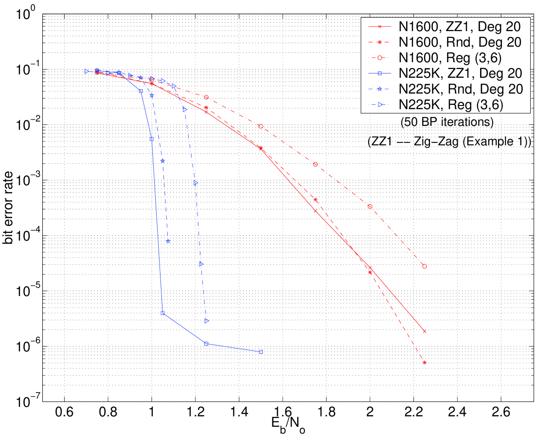
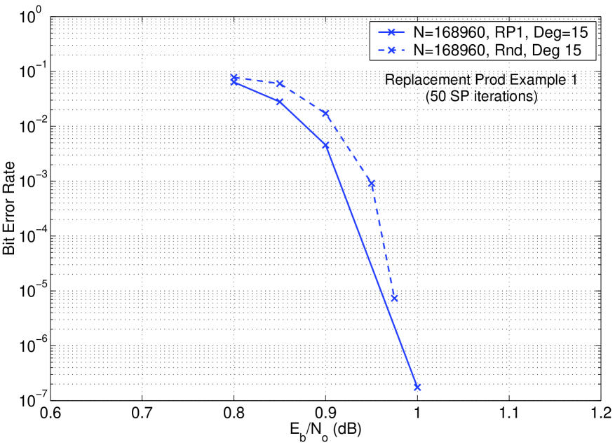
Figure 6 shows the performance of zig-zag product LDPC codes based on Example 4.2, with sum-product decoding. Once again, this performance is compared with the analogous performance of a LDPC code based on a random graph using identical sub-code constraints and having the same block length and rate. These results are also compared with a $(3,6)$ regular LDPC code that uses simple parity check constraints. For the parameters $p=3$ and $k=5$ in Example 4.2, a bipartite graph, based on the zig-zag product graph, on $768$ vertices with degree 20 is obtained. Using the $[20,15,4]$ sub-code constraints as earlier, a block length 7680 rate 1/2 LDPC code is obtained. This code performs comparably with the random LDPC code that is based on a degree 20 randomly designed graph. Using the parameters $p=5$ and $k=4$ and a $[16,12,2]$ sub-code, a longer block length 122,880 LDPC code is obtained. As in the previous case, this code also performs comparably, if not, better than its random counterpart for low to medium signal-to-noise ratios (SNRs). Once again, we attribute its slightly inferior performance at high SNRs to the poor girth of the zig-zag product graph.

Figure 7 shows the performance of a replacement product LDPC code based on Example 4.2, with sum-product decoding. Once again, this performance is compared with the analogous performance of an LDPC code based on a random graph using identical sub-code constraints and having the same block length and rate. For the parameters $p=5$ and $k=13$ in Example 4.2, a bipartite graph, based on the replacement product graph, on $15,360$ vertices with degree 15 is obtained. Using the $[15,11,3]$ Hamming code as a sub-code in the replacement product graph, a block length 115,200 rate 0.4667 LDPC code is obtained. The performance of the replacement product LDPC code is inferior to that of the random code in this example due to the poor choice of the generators in the component Cayley graphs. We believe a more judicious choice would improve the performance considerably.

Figure 6. LDPC codes from zig-zag product graphs based on Example 4.2.

Figure 7. LDPC code from replacement product based on Example 4.2.

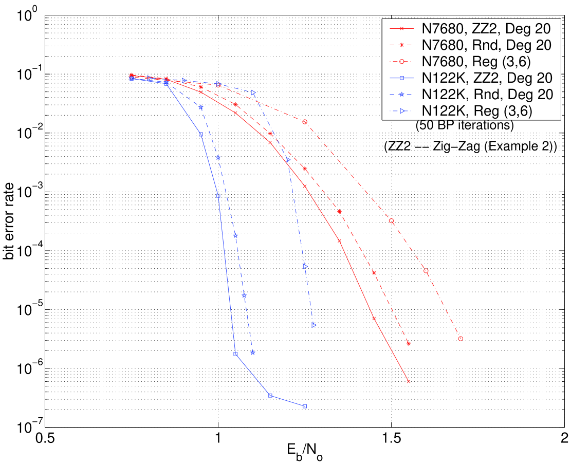
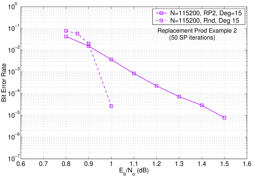
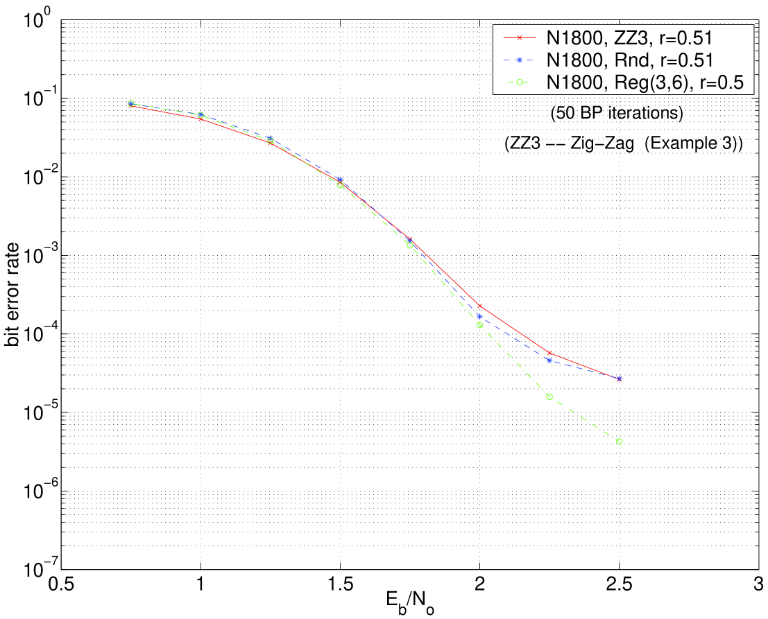
Figure 8 shows the performance of LDPC codes designed based on the zig-zag product of two unbalanced bipartite graphs as in Example 4.3. A $(6,10)$-regular bipartite graph on $(20,12)$ vertices is chosen as one of the component graphs and a $(3,5)$-regular bipartite graph on $(10,6)$ vertices is chosen as the other component. Their zig-zag product is a $(9,25)$-regular bipartite graph on $(200,72)$ vertices. Using sub-code constraints of two codes – a $[9,6,2]$ and a $[25,21,2]$ linear block code – a block length 1800 LDPC code of rate 0.5066 is obtained. The performance of this code is compared with a LDPC code based on a random $(9,25)$-regular bipartite graph using the same sub-code constraints, and also with a block length 1800 random $(3,6)$ regular LDPC code. All three codes perform comparably, with the random $(3,6)$ showing a small improvement over others at high SNRs. Given that the zigzag product graph is composed of two very small graphs, this result highlights the fact that good graphs may be designed using just simple component graphs.

Figure 8. LDPC code from the unbalanced bipartite zig-zag product graph based on Example 4.3.

7. Iterative construction of generalized product graphs

In this section, we introduce iterative families of expanders that address an important design problem in graph theory and that have several other practical engineering applications such as in designing communication networks, complexity theory, and derandomization techniques.

For code constructions, we would ideally use products that could be iterated to generate families of LDPC codes having a slow growth in the number of vertices (so as to get codes for many block-lengths), while maintaining a constant (small) degree. The iterative families described in this section have these characteristics, but unfortunately do not have parameters that make the codes practical. Designing such iterative constructions suitable for coding is a nice open problem.

First we review the iteration scheme of [13] for the original zig-zag product starting from a seed graph $H$. The existence of the seed graph $H$ as well as explicit examples of suitable seed graphs for $H$ are also discussed in [13]. We present new iterative constructions of a modified unbalanced bipartite zig-zag product and the replacement product thereafter.

7.1. Iterative construction of original zig-zag product graphs

We will need a squaring operation and the zig-zag operation in the iterative technique that is proposed next. Note that for a graph $G$, its square $G^{2}$ is a graph whose vertices are the same as in $G$ and whose edges are paths of length two in $G$. Further, if $G$ is a $(N,D,\lambda)$ graph, then $G^{2}$ is a $(N,D^{2},\lambda^{2})$ graph.

A graph $H$ is used to serve as the basic building block for the iteration. Let $H$ be any $(D^{4},D,\frac{1}{5})$ graph. Then the iteration is defined by

$$G_{1}=H^{2}=(D^{4},D^{2},\frac{1}{25}).$$

$$G_{i+1}=G_{i}^{2}\mbox{\scriptsize$Z$⃝}H.$$

The above iterative construction indeed gives a family of expanders as presented in the following result:

Theorem 2.

[13] For every $i$, $G_{i}$ is an $(D^{4i},D^{2},\frac{2}{5})$ graph.

7.2. Iterative construction of unbalanced bipartite zig-zag product graphs

The unbalanced bipartite zig-zag product presented in Section 4 cannot be used directly to obtain an iterative construction, due to constraints on the parameters. Therefore, we slightly modify the zig-zag product by introducing an additional step on the small component graph in the product construction. We note that the introduction of this additional step can only increase the expansion of the zig-zag product graph. However, this increase in expansion is at the cost of increasing the degree of the graph slightly. The new modified unbalanced bipartite zig-zag product is presented next, followed by an iterative construction that uses this product.

7.2.1. Modified unbalanced bipartite zig-zag product

The two component graphs are unbalanced bipartite graphs, i.e., the two sets of vertices have different degrees. Let $G_{1}$ be a $(c_{1},d_{1})$-regular graph on the vertex sets $V_{1},W_{1}$, where $|V_{1}|=N$ and $|W_{1}|=M$. Let $G_{2}$ be a $(c_{2},d_{2})$-regular graph on the vertex sets $V_{2},W_{2}$, where $|V_{2}|=d_{1}$ and $|W_{2}|=c_{1}$. Let $\lambda_{1}$ and $\lambda_{2}$ denote the second largest eigenvalues of the normalized adjacency matrices of $G_{1}$ and $G_{2}$, respectively. Again, randomly number the edges around each vertex $\tilde{v}$ in $G_{1}$ and $G_{2}$ by $\{1,\ldots,deg(\tilde{v})\}$, where $deg(\tilde{v})$ is the degree of $\tilde{v}$. Then the zig-zag product graph, which we will denote by $G=G_{1}\mbox{\tiny$Z_M$⃝}G_{2}$, is a $(c_{2}^{2}d_{2},d_{2}^{2}c_{2})$-regular bipartite graph on the vertex sets $V,W$ with $|V|=N\cdot d_{1}$, $|W|=M\cdot d_{1}$, formed in the following manner:

• Every vertex $v\in V_{1}$ and $w\in W_{1}$ of $G_{1}$ is replaced by a copy of $G_{2}$. The cloud at a vertex $v\in V_{1}$ has vertices $V_{2}$ on the left and vertices $W_{2}$ on the right, with each vertex from $W_{2}$ corresponding to an edge from $v$ in $G_{1}$. The cloud at a vertex $w\in W_{1}$ is similarly structured with each vertex in $V_{2}$ in the cloud corresponding to an edge of $w$ in $G_{1}$. (See Figure 3.) Then the vertices from $V$ are represented as ordered pairs $(v,k)$, for $v\in\{1,\dots,N\}$ and $k\in\{1,\dots,d_{1}\}$, and the vertices from $W$ are represented as ordered pairs $(w,\ell)$, for $w\in\{1,\dots,M\}$ and $\ell\in\{1,\dots,c_{1}\}$.

• A vertex $(v,k)\in V$ is connected to a vertex in $W$ by making four steps in the product graph. The first three steps are the same as in Section 4. The fourth step is:

  • A second small step from right to left in the local copy of $G_{2}$. This is a step $(v[k[i]],\ell[j])\rightarrow(v[k[i]],\ell[j][j^{\prime}])$, where the final vertex is in $W$, for $j^{\prime}\in\{1,\ldots,d_{2}\}$.

  Therefore, there is an edge between $(v,k)$ and $(v[k[i]],\ell[j][j^{\prime}])$.

Theorem 3.

Let $G_{1}$ be a $(c_{1},d_{1})$-regular bipartite graph on $(N,M)$ vertices with $\lambda(G_{1})=\lambda_{1}$, and let $G_{2}$ be a $(c_{2},d_{2})$-regular bipartite graph on $(d_{1},c_{1})$ vertices with $\lambda(G_{2})=\lambda_{2}$. Then, the modified zig-zag product graph $G_{1}\mbox{\tiny$Z_M$⃝}G_{2}$ is a $(c_{2}^{2}d_{2},c_{2}d_{2}^{2})$-regular bipartite on $(N\cdot d_{1},M\cdot d_{1})$ vertices with $\lambda=\lambda(G_{1}\mbox{\tiny$Z_M$⃝}G_{2})\leq\lambda_{1}+\lambda_{2}+\lambda_{2}^{2}$. Moreover, if $\lambda_{1}<1$ and $\lambda_{2}<1$, then $\lambda=\lambda(G_{1}\mbox{\tiny$Z_M$⃝}G_{2})<1$.

The proof is omitted but may be seen intuitively given the expansion of the original unbalanced zig-zag product (Theorem 1) in the following way. The new step is independent of the previous steps and is essentially a random step on an expander graph ($G_{2}$). Considering a distribution on the vertices $(v,k)$ of $G=G_{1}\mbox{\tiny$Z_M$⃝}G_{2}$, if the distribution of $k$ conditioned on $v$ is close to uniform after step 3, then step 4 is redundant and no gain is made. If the distribution of $k$ conditioned on $v$ is not close to uniform after step 3, then step 4 will increase the entropy of $k$ by the expansion of $G_{2}$.

7.2.2. Iterative construction

The modified zigzag product of $G_{1}=(N,M,c_{1},d_{1},\lambda_{1})$ and $G_{2}=(d_{1},c_{1},c_{2},d_{2},\lambda_{2})$ is a graph $G=G_{1}\mbox{\tiny$Z_M$⃝}G_{2}$ that is $(c_{2}^{2}d_{2},c_{2}d_{2}^{2})$-regular on $(Nd_{1},Md_{1})$ vertices. For the iteration, let $H$ be any $(N=c_{2}^{4}d_{2}^{5},M=c_{2}^{5}d_{2}^{4},c_{2},d_{2},\lambda)$ expander graph, Then, the iteration is defined by

$$G_{1}=H^{3}=(N,M,c_{2}^{2}d_{2},c_{2}d_{2}^{2},\lambda^{3}).$$

$$G_{i+1}=G_{i}^{3}\mbox{\tiny$Z_M$⃝}H.$$

We show that the above iterative technique yields a family of expanders in the following

Theorem 4.

Let $H$ be a $(c_{2}d_{2}^{2},c_{2}^{2}d_{2},c_{2},d_{2},\lambda)$ graph, where $\lambda\leq 0.296$. Let $G_{1}=H^{3}$ and $G_{i+1}=G_{i}^{3}\mbox{\tiny$Z_M$⃝}H$. Then the $i$-th iterated zig-zag product graph $G_{i}$ is a $((c_{2}^{4i}d_{2}^{5i},c_{2}^{4i+1}d_{2}^{5i-1},c_{2}^{2}d_{2},c_{2}d_{2}^{2},\lambda^{\prime})$ graph, where $\lambda^{\prime}\leq 0.55$.

Proof.

Let $n_{i}$ and $m_{i}$ be the number of left vertices and right vertices in $G_{i}$, respectively. Since $G_{i}=G_{i-1}^{3}\mbox{\tiny$Z_M$⃝}H$, we have $n_{i}=n_{i-1}(c_{2}^{4}d_{2}^{5})$ and $m_{i}=m_{i-1}(c_{2}^{4}d_{2}^{5})$. Since $n_{1}=c_{2}^{4}d_{2}^{5}$ and $m_{1}=c_{2}^{5}d_{2}^{4}$, it follows from the above recursion that $n_{i}=c_{2}^{4i}d_{2}^{5i}$ and $m_{i}=c_{2}^{4i+1}d_{2}^{5i-1}$. Note that $G_{i}$ is always $(c_{2}^{2}d_{2},c_{2}d_{2}^{2})$-regular.

Let $\lambda_{i}$ be the normalized second eigenvalue of $G_{i}$. Using the result from Theorem 3, we have

$$\lambda_{i}\leq\lambda_{i-1}^{3}+\lambda+\lambda^{2}.$$

Further note that $\lambda_{1}=\lambda^{3}$. Observe that even for $\lambda_{i}=\lambda_{i-1}^{3}+\lambda+\lambda^{2}$, the series converges $\lambda_{i}\rightarrow 0.5499$ when $\lambda\leq 0.296$. Hence, for each iteration $i$, $\lambda_{i}\leq 0.55$, thereby yielding a family of expanders. ∎

7.3. Iterative construction of replacement product graphs

The replacement product of $G_{1}=(N,d_{1},\lambda_{1})$ and $G_{2}=(d_{1},d_{2},\lambda_{2})$, denoted by $G_{1}\mbox{\scriptsize$R$⃝}G_{2}$, is an $(Nd_{1},d_{2}+1,\lambda)$ graph. In [13], it is shown that the expansion of the replacement product graph is given by

$$\lambda\leq(p+(1-p)f(\lambda_{1},\lambda_{2}))^{\frac{1}{3}},\hskip 108.405pt$$ (1)

$$\mbox{ where }p=\frac{d_{2}^{2}}{(d_{2}+1)^{3}}\mbox{ and }f(\lambda_{1},\lambda_{2})=\frac{1}{2}(1-\lambda_{2}^{2})\lambda_{1}+\frac{1}{2}\sqrt{(1-\lambda_{2}^{2})^{2}\lambda_{1}^{2}+4\lambda_{2}^{2}}.$$

To obtain an iterative construction, we choose two graphs $G_{1}=(N,(d+1),\lambda_{1})$ and $H=((d+1)^{4},d,\lambda_{2})$.

The iteration is defined by

$$G_{i+1}=(G_{i})^{4}\mbox{\scriptsize$R$⃝}H.$$

We show that the above iterative construction results in a family of expanders.

Theorem 5.

Let $G_{1}$ be a $(N,(d+1),\lambda_{1})$ graph and let $H$ be a $((d+1)^{4},d,\lambda_{2})$ graph, where $\lambda_{1}\leq 0.2,\lambda_{2}\leq 0.2$ and $d\geq 6$. Let $G_{i+1}=(G_{i})^{4}\mbox{\scriptsize$R$⃝}H$. Then the $i$-th iterated replacement product graph $G_{i}$ is a $(N(d+1)^{4(i-1)},d+1,\lambda)$ graph, where $\lambda\leq 0.86$.

Proof.

Let $n_{i}$ be the number of vertices in $G_{i}$. Then $n_{i}=n_{i-1}(d+1)^{4}$. Since $n_{1}=N$, it follows that $n_{i}=N(d+1)^{4i-4}$. It is clear that the degree of $G_{i}$ is one more than the degree of $H$, and thus, $G_{i}$ is $(d+1)$-regular. Let $\lambda_{i}$ be the normalized second eigenvalue of $G_{i}$. Using the result from Equation (1), we have

$$\lambda_{i}\leq[p+(1-p)f(\lambda_{i-1}^{4},\lambda_{2})]^{\frac{1}{3}},$$

where $p=\frac{d^{2}}{(d+1)^{3}}$ and $f$ is as above. Using numerical methods with Matlab, it was verified that $\lambda_{i}$ converges to $0.8574$ when $\lambda_{1}\leq 0.2,\lambda_{2}\leq 0.2$, and $d\geq 6$. Hence, for each iteration $i$, $\lambda_{i}<0.86$, thereby yielding a family of expanders. ∎

Note that if the above iteration was defined to be $G_{i+1}=(G_{i})^{2}\mbox{\scriptsize$R$⃝}H$, then for no choice of $\lambda_{1},\lambda_{2}$, or $d$, would the resulting iterative family be expanders.

8. Conclusions

In this paper we generalized the zig-zag product resulting in a product for unbalanced bipartite graphs. We proved that the resulting graphs are expander graphs as long as the component graphs are expanders. We examined the performance of LDPC codes obtained from zig-zag and replacement product graphs. The resulting product LDPC codes perform comparably to random LDPC codes with the additional advantage of having a compact description. We also introduced iterative constructions for the unbalanced zig-zag and replacement products yielding families of graphs with small, constant or slowly increasing degrees, and good expansion. Although these iterative schemes do not yield parameters for practical codes as yet, we believe they provide a first step in exploring iterated products for code construction. Designing iterative graph products that result in a family of good practical codes remains an intriguing open problem. We conclude that codes from product graphs provide a nice avenue for code constructions.

Submitted: August 17, 2007.

References

- [1] N. Alon. Eigenvalues and expanders. Combinatorica, 6(2):83–96, 1986. Theory of computing (Singer Island, Fla., 1984).
- [2] N. Alon, A. Lubotzky, and A. Wigderson. Semi-direct product in groups and zig-zag product in graphs: connections and applications (extended abstract). In 42nd IEEE Symposium on Foundations of Computer Science (Las Vegas, NV, 2001), pages 630–637. IEEE Computer Soc., Los Alamitos, CA, 2001.
- [3] W. Imrich and S. Klavžar. Product graphs. Wiley-Interscience Series in Discrete Mathematics and Optimization. Wiley-Interscience, New York, 2000. Structure and recognition, With a foreword by Peter Winkler.
- [4] H. Janwa and A. K. Lal. On Tanner codes: minimum distance and decoding. Appl. Algebra Engrg. Comm. Comput., 13(5):335–347, 2003.
- [5] C. Kelley, J. Rosenthal, and D. Sridhara. Some new algebraic constructions of codes from graphs which are good expanders. In Proc. of the 41-st Allerton Conference on Communication, Control, and Computing, pages 1280–1289, 2003.
- [6] C. Kelley and D. Sridhara. Eigenvalue bounds on the pseudocodeword weight of expander codes. Journal of Advances in Mathematics of Communication, Aug. 2007.
- [7] J. Lafferty and D. Rockmore. Codes and iterative decoding on algebraic expander graphs. In the Proceedings of ISITA 2000, Honolulu, Hawaii, available at http://www-2.cs.cmu.edu/afs/cs.cmu.edu/user/lafferty/www/pubs.html, November 2000.
- [8] N. Linial and A. Wigderson. Expander graphs and their applications. Lecture notes of a course given at the Hebrew University, 2003. Available under http://www.math.ias.edu/avi/TALKS/.
- [9] A. Lubotzky. Discrete Groups, Expanding Graphs and Invariant Measures. Birkhäuser Verlag, Basel, 1994. With an appendix by Jonathan D. Rogawski.
- [10] A. Lubotzky, R. Phillips, and P. Sarnak. Ramanujan graphs. Combinatorica, 8(3):261–277, 1988.
- [11] G. A. Margulis. Explicit group-theoretic constructions of combinatorial schemes and their applications in the construction of expanders and concentrators. Problems Inform. Transmission, 24(1):39–46, 1988. Translation from Problemy Peredachi Informatsii.
- [12] R. Meshulam and A. Wigderson. Expanders in group algebras. Combinatorica, 2003. To appear.
- [13] O. Reingold, S. Vadhan, and A. Wigderson. Entropy waves, the zig-zag graph product, and new constant-degree expanders. Ann. of Math. (2), 155(1):157–187, 2002.
- [14] J. Rosenthal and P. O. Vontobel. Constructions of LDPC codes using Ramanujan graphs and ideas from Margulis. In Proc. of the 38-th Allerton Conference on Communication, Control, and Computing, pages 248–257, 2000.
- [15] M. Sipser and D. A. Spielman. Expander codes. IEEE Trans. Inform. Theory, 42(6, part 1):1710–1722, 1996.
- [16] R. M. Tanner. A recursive approach to low complexity codes. IEEE Trans. Inform. Theory, 27(5):533–547, 1981.
- [17] R. M. Tanner. Explicit concentrators from generalized -gons. SIAM J. Algebraic Discrete Methods, 5(3):287–293, 1984.
- [18] J.-P. Tillich and G. Zémor. Optimal cycle codes constructed from Ramanujan graphs. SIAM J. Discrete Math., 10(3):447–459, 1997.
- [19] J. K. Wolf. Efficient maximum likelihood decoding of linear block codes using a trellis. IEEE Trans. Inform. Theory, IT-24(1):76–80, 1978.