A Generic Global Constraint based on MDDs

Abstract

The paper suggests the use of Multi-Valued Decision Diagrams (MDDs) as the supporting data structure for a generic global constraint. We give an algorithm for maintaining generalized arc consistency (GAC) on this constraint that amortizes the cost of the GAC computation over a root-to-terminal path in the search tree. The technique used is an extension of the GAC algorithm for the regular language constraint on finite length input[19]. Our approach adds support for skipped variables, maintains the reduced property of the MDD dynamically and provides domain entailment detection. Finally we also show how to adapt the approach to constraint types that are closely related to MDDs, such as AOMDDs [17] and Case DAGs [7].

1 Introduction

Constraint Programming (CP)[21] is a powerful technique for specifying Constraint Satisfaction Problems (CSPs) based on allowing a constraint programmer to model problems in terms of high-level constraints. Using such global constraints allows easier specification of problems but also allows for faster solvers that take advantage of the structure in the problem. The classical approach to CSP solving is to explore the search tree of all possible assignments to the variables in a depth-first search backtracking manner, guided by various heuristics, until a solution is found or proven not to exist. One of the most basic techniques for reducing the number of search tree nodes explored is to perform domain propagation at each node. In order to get as much domain propagation as possible we wish for each constraint to remove from the variable domains all values that cannot participate in a solution to that constraint. This property is known as Generalized Arc Consistency (GAC). It is only possible to achieve GAC for some types of global constraints in practice, as some global constraint model NP-hard problems making GAC infeasible. The use of global constraints can significantly reduce the total number of constraints in the model, which again improves domain propagation if GAC or other powerful types of consistency can be enforced. However, in typical CSPs there are many constraints that lie outside the domain of the current Global Constraints. Such constraints are typically represented as a conjunction of simple logical constraints or stored in tabular form. The former can potentially cause a massive loss in domain propagation efficiency, while the tabular constraints typically takes up too much space for all but the most simple constraints and for the same reason performing domain propagation can be expensive. We aim to introduce a new generic global constraint type for constraints on finite domains based on the approach of compiling an explicit, but compressed, representation of the solution space of as many constraints as possible. To this end we suggest the use of Multi-Valued Decision Diagrams (MDDs). It is already known how to perform GAC in linear, or nearly linear time in the size of the decision diagram for many types of decision diagrams including MDD’s[6, 17, 12]. However, compact as decision diagrams may be, they are still of exponential size in the number of variables in the worst case. In practice their size is also the main concern, even when they do not exhibit worst case behavior. Applying the static GAC algorithms at every step of the search is therefore likely to cause an unacceptable overhead in many cases. To avoid this it is essential to avoid repeating computation from scratch at each step and instead use an algorithm that amortizes the cost of the GAC computation over a number of domain propagation steps. In this paper we introduce such an algorithm. In section 2 we discuss compiling versus searching. Section 3 defines the type of search we consider and the operations our constraint will support. In section 4.1 we describe the standard GAC algorithm for MDDs based on scanning the entire data structure and also cover some optimizations available from related work. In section 5 we present a basic dynamic approach for a simplified version of the MDD data structure based on the technique used in [19] and contrast it to the scanning approach covered in the preceding section. In Section 6 and 7 we extend the dynamic approach to support MDDs fully as well as provide domain entailment detection. In Section 8 we discuss the issue of constructing the MDD constraints. Finally in Section 9 we show how to apply our techniques to some other data structures that can be viewed as a compilation of the solution space.

1.1 Related Work

The concept of compiling an explicit, but compact, representation of the solution space of a set of constraints has previously been applied to obtain backtrack-free configurators for many practical configuration problems[14]. In this case Binary Decision Diagrams (BDDs)[6] are used for representing the solution space. However, it is well known that BDDs(and MDDs) are not generally capable of efficiently representing constraints where the allowable values of a variable depends on all the preceding variables as it is then very hard to obtain good substructure sharing. This means that prominent constraints such as the AllDifferent constraint[20] cannot be represented in practice unless the number of variables is very small. Techniques have been developed for achieving GAC in BDDs under the restriction of an external constraint, but as we show in section 2 this technique cannot be applied when the external constraint is the AllDifferent constraint. This motivates a compromise between compilation and search, such as it is achieved by the MDD global constraint presented in this paper.

The regular language constraint for finite sequences of variables is introduced in [19]. It uses a DFA to represent the valid inputs where the input is limited to be of length $n$. Since the constraint considers a finite number of inputs, these can be mapped to $n$ variables, and the constraint can be made Generalized Arc Consistent according to these variables domains. To this end the cycles in the DFA are ’unfolded’ by taking advantage of the fact that the input is of a finite length. The resulting data structure has size $O(nd_{max}q)$ where $n$ is the number variables, $q$ the number of states in the DFA and $d_{max}$ the size of the largest variable domain. A GAC algorithm that amortizes the cost of the GAC computation over root-to-leaf paths in the search tree based on this data structure is also presented. We note that there is a strong correspondence between the unfolded DFA and an MDD representing the same constraint, but there are some important extra requirements on the MDD structure which we take into account in this paper. However, the GAC algorithm on the unfolded DFA in the regular constraint still forms the basis of our GAC algorithm for the MDD. Below we summarize our new contributions and highlight the differences compared to the regular constraint.

• DFAs do not allow skipping inputs, even for states where the next input is irrelevant. Skipping input variables in this manner is part of the reduce steps for BDDs, and if used in MDDs requires alterations to the GAC algorithm. We give a modified algorithm to handle this. In some cases allowing the decision diagram to skip variables can give a significant reduction in size. A very simple example is a constraint specifying that the value $v$ must occur at least once for one of the variables $x_{1},\ldots,x_{n}$. In an MDD that does not allow skipped variables(or an unfolded DFA) this requires $\Omega(n^{2})$ nodes compared to $O(n)$ nodes if we allow skipped variables in the MDD.

• BDDs are normally kept reduced during operations on the BDDs. This allows subsequent operations to run faster and also shows directly if the result is the constant true function. We present an approach that can dynamically reduce the MDD without resorting to scanning the entire live part of the data structure, and which also allows us to detect domain entailment [26]. Such entailment detection can be a very important property of a global constraint as it can save processing of the entailed constraint in all descendant search nodes. We note that implemented state-of-the-art CSP solvers, such as GeCode[3], allow constraints to signal entailment in order to optimize the search process.

  The suggestion in [19] is to minimize the DFA only once at the beginning (thereby also minimizing the initial ’unfolded’ DFA) which would correspond to reducing the MDD prior to the search, and does not provide any form of entailment detection. The problem of efficient dynamic minimization is not discussed in [19] and would seem to require a technique similar to the one we present in this paper for obtaining dynamic reduction of the MDD constraint.

• We adapt the GAC algorithm to operate on other decision diagram style data structures such as AOMDDs [17] and Case DAGs [7].

Finally, from a practical perspective its not a good idea to first construct a DFA and then unfold it. It is more efficient to use a BDD package to construct an ROBDD directly, as efficient BDD packages [1, 2] with a focus on optimizing the construction phase have already been developed driven by needs in formal verification [18]. Specifically the use of BDDs for the construction gives access to the extensive work done on variable ordering (see for example [4, 15, 22]) for BDDs. Once an ROBDD is constructed it can then easily be converted into the desired MDD.

Another related result is [9] in which it is discussed how to maintain Generalized Arc Consistency in a binary decision diagram(BDD) when using the BDD as a global constraint in a CSP. The solution approach suggested in [9] is intended for smaller constraints with a small scope, and is only presented for the case of binary variables. Their technique differs from the straightforward scanning technique by using shared good/no-good recording and a simple cut-off technique to (in some cases) reduce the amount of nodes visited in a scan. Their technique can be adapted for non-binary variables, but good/no-good recording becomes useless as the scope of the MDD constraint increase, and the cut-off technique lose merit if we wish to reduce the MDD dynamically or have domains that are even slightly larger than 2. Hence their techniques do not apply when the intention is to collect as many small constraints as possible into one global MDD. We discuss the direct adaption of their technique to non-binary variables below and compare it to our approach in section 4.1.

An entirely different approach is suggested in [5, 11] which considers representing constraints as a disjunction of geometrical constraints(boxes and triangles in [11] and just boxes in [5]. The experiments in [11] gives a comparison with the case constraint[7] which is implemented using what is essentially an MDD, called a case DAG, where edges represents an interval of values. They also provide comparisons with using a case DAG directly along with a simple GAC algorithm that treats the DAG as a tree. The experiments show that the naive DAG approach is slower than the box and triangle approach, but the case implementation (which most likely uses a DFS scanning approach) is still faster. In section 9.1 we extend our dynamic approach to support the case DAG, most likely increasing the advantage over the box and triangle approach.

1.2 Notation

In this paper we consider a CSP problem $\textit{CP}(X,D,F)$, where $X=\{x_{1},\ldots,x_{n}\}$ is the set of variables, $F$ the set of constraints and $D=\{D_{1},\ldots,D_{n}\}$ is the multi-set of variable domains, such that the domain of a variable $x_{i}$ is $D_{i}$. When discussing a backtracking search we will use $D_{i}$ to refer to the currently allowed domain values for $x_{i}$, and $D_{i}^{0}$ to denote the original domains. We use $d_{i}=|D_{i}^{0}|$ to denote the size of domains and $d_{max}=\max\{d_{i}|x_{i}\in X\}$ to denote the largest domain (for simplifying complexity analysis). We use $scope(\{F_{1},\ldots,F_{j}\})$ and $scope(F_{j})\subseteq X$ to denote the variable scope of a set of constraints and a single constraint respectively.

A single assignment $a$ is a pair $(x_{i},v)$ where $x_{i}\in X$ and $v\in D^{0}_{i}$. The assignment $a$ is said to have support in a constraint $F_{k}$, iff there exists a solution to $F_{k}$ where $x_{i}$ is assigned $v$. If a single assignment ($x_{i},v$) has support in a constraint $F_{j}$, $v$ is said to be in the valid domain for $x_{i}$, denoted $VD_{i}(F_{j})$. If for all variables $x_{i}$ and a constraint $F_{j}$ it is the case that $D_{i}=VD_{i}(F_{j})$ then $F_{j}$ is said to fulfill the property of Generalized Arc Consistency (GAC). A partial assignment $\rho$ is a set of single assignments to distinct variables, and a full assignment is a partial assignment that assigns all variables.

1.3 The MDD data structure

Below we give the definition of the MDD data structure. We will then present the valid domains algorithm and show how to store the MDD to support the suggested algorithms.

Definition 1 (Ordered Multi-Valued Decision Diagram (OMDD)).

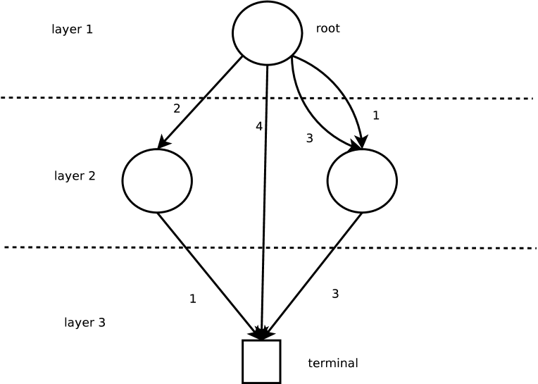
An Ordered Multi-Valued Decision Diagram (OMDD or just MDD) for a CSP CP is a layered Directed Acyclic MultiGraph $G(V,E)$ with up to $n+1$ layers. Each node $u$ has a label $l(u)\in\{1,\ldots,n+1\}$ corresponding to the layer in which the node is placed, and each edge $e$ outgoing from layer $i$ has a label $v(e)\in D_{i}$. Furthermore we use $s(e)$ and $d(e)$ to denote the source and destination layer of each edge $e$ respectively.

The following restrictions apply:

• There is exactly one node $u$ such that $l(u)=\min\{l(q)\mid q\in V\}$ denoted root.

• There is exactly one node $u$ such that $l(u)=n+1$ denoted terminal.

• For any node $u$, all outgoing edges from $u$ have distinct labels.

• All nodes except $terminal$ has at least one outgoing edge.

• For all $e\in E$ it is the case that $s(e)<l(e)$.

A full assignment $\rho$ is a solution to a given MDD iff there exists a path $Q=(e_{1},\ldots,e_{j})$ from root to terminal such that for each $(x_{i},v)\in\rho$ there exists an edge $e\in Q$ such that $l(e)=i$ and $v(e)=v$ or $s(e)<i<d(e)$.

Figure 1: The above figure shows an example MDD that is fully reduced. Assuming $D_{1}=\{1,2,3,4\}$ and $D_{2}=\{1,2,3\}$, it represents the binary constraint with solutions { (1,3),(2,1), (3,3),(4,1),(4,2),(4,3) }.

We will use $V_{i}=\{u\in V\mid l(u)=i\}$ to denote the nodes of layer $i$ and $E_{i}=\{e\in E\mid s(e)=i\}$ to denote the set of edges originating from layer $i$. Furthermore we define $P_{u}=\{(p,v)\mid\exists e\in E:v(e)=v\land s(e)=p\land d(e)=u\}$ and $C_{u}=\{(c,v)\mid\exists e\in E:v(e)=v\land s(e)=u\land d(e)=c\}$. That is, $P_{u}$ corresponds to the incoming edges to $u$, and $C_{u}$ corresponds to the outgoing edges of $u$.

Definition 2 (Reduced OMDD).

An MDD is called uniqueness reduced iff for any two distinct nodes $u_{1},u_{2}$ at any layer $i$ it is the case that $C_{u_{1}}\not=C_{u_{2}}$.

If it is furthermore the case for all layers $i\in\{1,\ldots,n\}$ that no node $u_{1}$ in layer $i$ exists with $d_{i}$ outgoing edges to the same node $u_{2}$, the MDD is said to be fully reduced.

The above definitions are just the straightforward extension of the similar properties of BDDs[6]. Fully reduced MDDs retain the canonicity property of reduced BDDs, that is there is exactly one fully reduced MDD for each Boolean constraint on $n$ discrete domain variables. An example MDD is shown in Figure 1

2 Compiling vs. searching

Consider the problem of compiling the set of all possible solutions to a CSP. By compiling we mean computing an explicit, but compressed, representation of the set of solutions to the CSP, such that evaluation of assignments in time polynomial in the size of the representation is supported. While compiling the solution space is obviously harder than finding a single solution to the constraint set, this approach has been used successfully with BDDs for verification of circuits (as described above) and for interactive configuration[14]. That is, in certain scenarios it is possible to compile the entire solution space of a CSP problem which can be viewed as obtaining one huge global constraint upon which GAC can be enforced. There are of course many global constraint types which by themselves result in a decision diagram that is too large to handle. One of the most prominent is the AllDifferent constraint. As there are many practical applications where an AllDifferent constraint plays a crucial role (such as layout/placement problems, which also frequently occur in configuration problems) it seems obvious that a search approach is appropriate.

However, in a recent result [13] it was shown how to perform valid domains computation on a BDD under the further restriction of a separate linear constraint(which if included in the BDD might have produced an exponential blow-up in size) in polynomial time in the size of the BDD. This allows efficient cost configuration for a restricted class of cost functions. That is, in some cases it is possible to filter the valid domains computation enforcing additional constraints without encoding the additional constraints directly in the decision diagram. It is obvious to consider whether or not a similar approach can be taken for the problematic AllDifferent constraint. However, as we show below, performing valid domains computation under the restriction of an AllDifferent constraint in polynomial time in the size of the BDD implies that P=NP.

Theorem 3.

If an algorithm exists for checking satisfiability of the conjunction of an MDD and an AllDifferent constraint in time polynomial in the size of the MDD then P = NP.

Proof.

We consider the Hamiltonian Path problem[16] on an undirected graph $G(V_{H},E_{H})$. We will show that the Hamiltonian Path problem can be expressed as an AllDifferent constraint conjoined with an MDD of size polynomial in the number of nodes in the input graph. Therefore the existence of a polynomial time algorithm deciding whether or not an MDD contains a solution that satisfies an AllDifferent constraint implies P = NP.

We model the Hamiltonian path problem with $n=|V_{H}|$ variables of domain size $n$. The value of the $i$th variable corresponds to the $i$th node visited in the Hamiltonian path. We use an MDD to represent the N-Walk constraint, which restricts the values of the $n$ variables to represent a valid $n$ node long walk of the graph. That is, the edge labels of a path from root to terminal in the MDD gives a valid walk of $n$ steps in the graph $G_{H}$. An example is provided in Figure 2. When combined with an AllDifferent constraint over the $n$ variables, we have a representation of the Hamiltonian Path problem.

Figure 2: An example of an MDD encoding an N-Walk constraint. On the left is shown an example graph, and on the right the corresponding MDD. In order to avoid clutter some edge labels have been left out in the MDD and instead edges leading to a node labelled for example “1”,”2”,”3” or “4” correspond to edge labels 1,2,3 and 4 respectively (this type of labelling is only possible because all edges leading to the same MDD node always have the same label in the N-Walk constraint). The root represents the choice point for the start of the walk, and nodes in layer 1 represents the choice point for the second node in the walk.

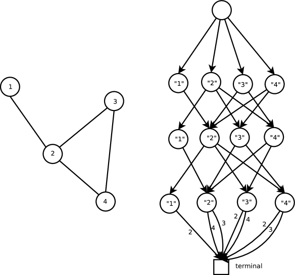
There are only $O(n^{2})$ different states in the N-Walk constraint, as the valid choices for the current variable depend only on the value of the preceding variable (the node in $G_{H}$ we are at now) and the number of variables already assigned (how many nodes have been visited so far). Hence the MDD representation is obviously polynomial, having at most $O(n^{2})$ nodes and at most $O(n^{3})$ edges, assuming it is uniqueness reduced. ∎

From this result we get a strong motivation for settling on a search strategy. One could argue that alternative compiled data structures providing valid domains computation under the restriction of an AllDifferent constraint in polynomial time of its size could exist. However, it is obvious from the above result that any such data structure must require super polynomial construction time in the worst-case when encoding the simple N-Walk constraint (unless $P=NP$).

3 Searching with an MDD

In this paper we consider a backtracking search for a solution to a conjunction of constraints at least one of which is an MDD. To simplify the complexity analysis, we assume that the search branches on the domain values of each variable in some specified order and that full domain propagation takes place after each branching. The process of branching and performing full domain propagation we will refer to as a phase. For the proposed constraint we refer to performing domain propagation on the MDD, as a single step. As such, one phase may contain many steps depending on how many iterations it takes until none of the constraints are able to remove any further domain values.

In order to be useful in this type of CSP search, an implementation of the MDD constraint needs to supply the following functionality:

• Assign($x,v$)

• Remove($(x_{1},v_{1}),\ldots,(x_{k},v_{k})$)

• Backtrack()

The Assign operation restricts the valid domain of $x$ to $v$ and is used to perform branchings. The Remove operation corresponds to domain restrictions occurring due to domain propagation in the other constraints. The Backtrack operations undoes the last Assign operation and all Remove operations that has occurred since, effectively backtracking one phase in the search tree.

For the implementation of Backtrack we will simply push data structure changes on a stack, so that they can be reversed easily when a backtrack is requested. This very simple method ensures that a backtrack can be performed in time linear in the number of data structure changes made in the last step. For all the dynamic data structures considered in this paper the space used for this undo stack will be asymptotically bounded by the time used over a root-to-terminal path in the search tree. Furthermore, in all the cases studied in this paper, Assign($x,v$) is just as efficiently implemented as a single call to Remove($\{(x_{i},v_{j})\mid v_{j}\in D_{i}\setminus\{v\}\}$). Therefore we will only discuss implementation of Remove.

4 Calculating the change in valid domains

In this section we consider two different approaches for determining which values are lost from the valid domains when applying restrictions of the form $x_{i}\not=v$. A crucial element in computing the valid domains is that of a supporting edge. An edge $e$ supports a single assignment $(x_{i},v)$, if $s(e)=i$ and $v(e)=v$ or $s(e)<i<d(e)$. Note that the existence of an edge supporting a give assignment implies that the assignment is part of the valid domain for the corresponding variable.

The first approach to maintaining valid domains we cover is the straight forward scanning approach that builds the valid domains from scratch by scanning and finding all supporting edges. In addition to this we discuss the direct adaptation of some optimization techniques from [9]. The second approach is the dynamic technique we suggest based on [19], which instead relies on tracking the loss of supporting edges.

Finally, to ease presentation we will at first assume that the OMDD we operate on is initially Uniqueness Reduced, but not fully reduced, in fact we will assume that all outgoing nodes from a node in layer $i$ lead to nodes in layer $i+1$ (and hence also $l(root)=1$). In section 6 we show how to handle a fully reduced OMDD.

4.1 The full scan algorithm

We will now present the standard scanning algorithm for computing the valid domains from scratch. It scans the MDD for supporting edges and stores the assignments that they support. This is done in a DFS manner deleting encountered edges that correspond to disallowed assignments. A node $u$ is said to die when it can no longer participate in any solution, and is otherwise said to be alive. During the DFS search nodes that are not already known to be dead or alive are searched recursively, and as soon as a valid path to terminal is found they are marked as being alive. A domain value is added to the valid domains if an edge with a live end point corresponding to this value is visited. The pseudo-code for this approach is shown in Figure 3.

• RemoveScan$(R)$
     1global $live\leftarrow\emptyset$ $\rhd$ Set of nodes found to be alive 2global $dead\leftarrow\emptyset$ $\rhd$ Set of nodes found to be (newly) dead 3for $i$ st. $x_{i}\in X$ 4 do$D_{i}\leftarrow\emptyset$ 5$rootAlive\leftarrow\textnormal{ScanRecursive}(root,R)$ 6if $rootAlive=false$ 7 then return Constraint failed

• ScanRecursive($u,R$)
      1if $u\in live$ 2 then return $true$ 3elseif $u\in dead$ 4 then return $false$ 5$alive\leftarrow false$ $\rhd$ $u$ is dead unless support is found 6for $(c,v)\in C_{u}$ $\rhd$ Outgoing edge from $u$ to $c$ 7 doif $c\in dead\lor(x_{l(u)},v)\in R$ 8 then $C_{u}\leftarrow C_{u}\setminus\{(c,v)\}$ $\rhd$ Edge is dead 9 elseif $\textnormal{ScanRecursive}(c,R)$ 10 then $alive\leftarrow true$ 11 $D_{l(u)}\leftarrow D_{l(u)}\cup\{v\}$ $\rhd$ Add to valid domain 12 else $C_{u}\leftarrow C_{u}\setminus\{(c,v)\}$ $\rhd$ Edge is dead 13if alive 14 then $live\leftarrow live\cup\{u\}$ 15 else $dead\leftarrow dead\cup\{u\}$ 16return $alive$

Figure 3: The above pseudo-code shows the scanning approach for the valid domains computation. The set $R$, i.e. the collection of arguments to Remove, consists of the pairs $(x_{i},v)$ that have been disallowed by other constraints since the last step. The set $dead$ consists of the nodes that have been found to be newly dead, while $live$ is the set of nodes that have been found to be alive in this step. The decremental updates to the outgoing edges $C_{u}$ can be implemented as marking in practice.

4.1.1 Two ways for nodes to perish

In order to analyze the complexity of the scanning algorithm it is important to distinguish between two different causes of a node $u$ dying. Firstly, all the parents of $u$ can lose their edge leading to $u$. If so, there is no longer any path from $root$ to $terminal$ through $u$, so $u$ can no longer be part of a solution. We will refer to this as a NoReference node death. Secondly, a node can lose all its outgoing edges, so that $root$ can never be reached from it, which we will call a NoValue node death. Similarly an edge dies if one of its end points die.

We will denote the set of live edges after the $i$’th step as $E^{i}_{liv}$. The initial edge set preceding the first step is $E^{0}$. Furthermore we use $E^{i}_{ref}$ to refer to the edges lost in step $i$ due to a NoReference node death. Similarly we will use $E^{i}_{val}$ to denote the set of edges that perished in step $i$ due to a $NoValue$ death. Note that an edge can appear in both $E^{i}_{ref}$ and $E^{i}_{val}$.

Lemma 4.

In step $t$ RemoveScan traverses $|E^{t}_{liv}|+|E^{t}_{val}\setminus E^{t}_{ref}|$ edges.

Proof.

We note that ScanRecursive when invoked on the root will visit all edges once except those that lie in a part of the MDD that cannot be accessed any more due to the new restriction in $R$. If an edge $e$ is inaccessible it must by definition at least die from NoReference, i.e. $e\in E^{t}_{ref}$. It follows that edges that die only from NoValue must be accessible and therefore will be traversed. ∎

4.1.2 Good/No-good recording

The use of good/no-good recording to assist the scan algorithm during search is introduced in [9]. The technique is extremely simple, relying on recording the current partial assignment projected on the scope of the constraint in question as a no-good when a backtrack is needed. If a partial assignment occurs that matches a previous failed partial assignment on the scope of the constraint, the constraint will know it has failed. This can also be done for the cases where no domains change, resulting in a ’good’ recording. Furthermore, the stored no-goods can be used by identical constraints defined on different scopes.

Obviously, the no-good recording is less useful if the constraints have a large scope, as the number of times the stored no-goods can potentially be used decreases exponentially as the scope increases.

4.1.3 $\Delta$-cutoff

This technique was suggested in [9] for use in BDDs, and consists of the following: While scanning we maintain the largest index $\Delta$ such that the currently discovered valid values in the domains of $x_{\Delta},\ldots x_{n}$ are the same as the valid values in the previous step. Should we at any time be scanning a node $v$ which has already been found to be alive( has at least one outgoing live edge to a live node), we can neglect to recursively scan its other children if $l(u)\geq\Delta$.

We expect $\Delta$-cutoff to be able to perform large cut-offs in a constraint with binary variable domains, but as the domain size increases, it will take much more scanning before a large continuous interval of variables find all the values they were previously allowed.

Furthermore, consider a node $s$ in the search tree. It might be the case that a cut-off is made that would otherwise have pruned a number of edges. As further restrictions are applied it is highly likely that we at some descendant search nodes of $s$ will be required to scan the part of the structure that was previously neglected. As there can be a large number of descendant search nodes the $\Delta$-cutoff might actually result in an non-constant factor performance decrease.

5 A New dynamic approach

In this section we present a dynamic algorithm for maintaining valid domains, based on tracking the loss of supporting edges to avoid recomputing the valid domains from scratch in every step. It follows the technique presented in [19], just applied to the MDD instead of the unfolded DFA. In the following sections we then extend the algorithm to handle fully reduced MDDs and add support for dynamically reducing the MDD, enabling us to deliver domain entailment detection.

5.1 Support lists

In order to avoid re-doing unnecessary work we track the set of supporting edges by storing a set of sets $S$, such that for every possible single assignment $(x_{i},v)$ where $x_{i}\in X$ and $v\in D_{i}$ there exists a set $s_{i,v}\in S$ containing all the nodes and the corresponding edges that gives support to the single assignment $(x_{i},v)$. As we will see below $S$ can easily be maintained. In maintaining $S$ we learn immediately when a single assignment no longer has support, as the corresponding $s_{i,v}$ list will be empty. Note that the space needed for the support lists is only $O(|E|)$.

5.2 Performing Remove

A remove operation is performed by, for each single assignment $(x_{i},v)$ to be removed, visit all nodes that offer support for $(x_{i},v)$. On each such node the update procedure RemoveEdge is used to remove the corresponding edge while maintaining $S$ and the valid domains. Both are shown in Figure 4.

• $\textnormal{Remove}(R)$
     1for each $(x_{i},v)\in R$ 2 dofor each $(u,c)\in s_{i,v}$ 3 $\textnormal{RemoveEdge}(u,c,v)$

• $\textnormal{RemoveEdge}(u,c,v)$
      1$C_{u}\leftarrow C_{u}\setminus\{(c,v)\}$ 2$P_{c}\leftarrow P_{c}\setminus\{(u,v)\}$ 3$s_{l(u),v}\leftarrow s_{l(u),v}\setminus\{(u,c)\}$ 4if $s_{l(u),v}=\emptyset$ 5 then $D_{l(u)}\leftarrow D_{l(u)}\setminus\{v\}$ 6 if $D_{l(u)}=\emptyset$ 7 then return Constraint failed 8if $C_{u}=\emptyset$ $\rhd$ $u$ dies a NoValue death 9 then for each $(p,v^{\prime})\in P_{u}$ 10 do$\textnormal{RemoveEdge}(p,u,v^{\prime})$ 11if $P_{c}=\emptyset$ $\rhd$ $c$ dies a NoReference death 12 then for each $(c^{\prime},v^{\prime})\in C_{c}$ 13 doRemoveEdge$(c,c^{\prime},v^{\prime})$

Figure 4: RemoveEdge takes as input the dead edge in form of the originating node $u$, the destination node $c$ and the corresponding value label $v$. It then moves from the dead edge downwards in depth first manner as long as there are nodes dying because of lack of references. If the node $u$ has no more outgoing edges it propagates upwards, removing nodes that have no more outgoing edges. Note that any call to RemoveEdge, except the initial one by Remove will only result in either upwards or downwards propagation. It is not possible to do both. This is because downwards propagation is only caused by nodes with no incoming edges, while upwards propagation is only caused by nodes with no outgoing edges. Furthermore the direction will remain the same after the initial invocation by Remove.

5.3 Complexity

We start by examining the complexity of Remove in terms of the number of calls to RemoveEdge. Ideally we would like an algorithm that never uses more time than the scanning approach per step, and gives an improved bound on the time spent in total. Finally we show how to choose data structures to support RemoveEdge in time $O(1)$ per call.

5.3.1 Worst case performance in a single step

Recall that a step corresponds to a request to apply generalized arc consistency which again corresponds to a call to Remove with a set of assignments banned by other constraints. The following result bounds the complexity of the Remove procedure in a single step.

Lemma 5.

The number of calls to RemoveEdge in the Remove in step $t$ is $|E^{t}_{ref}\cup E^{t}_{val}|$

Proof.

Consider the $\textnormal{RemoveEdge}(u,c,v)$ method. Assume it is called with an edge that has just died. Its then easy to see that it will only invoke RemoveEdge on edges that die as a consequence of the initial call. Since the first invocation of RemoveEdge in Remove is guaranteed to be on a dead edge, and since RemoveEdge maintains $S$, we can conclude that RemoveEdge is only called on newly dead edges. ∎

The dynamic algorithm can potentially use more time in a single step but we can give a (pessimistic) bound on how much slower the dynamic approach could be in total.

Lemma 6.

If RemoveScan visits $s$ edges in any given step $t$, then Remove causes at most $O(s)$ calls to RemoveEdge in step $t+1$.

Proof.

This is easily seen by the fact that any edges that die in a step, must have been alive in the previous step. Combining this with Lemma 4 and Lemma 5 yields the claim. ∎

Since there can potentially be a factor of $d_{max}$ more search nodes at step $t+1$ compared to step $t$, the above result means that the dynamic algorithm might theoretically work on a factor $d_{max}$ more edges in total. This is a natural consequence of the fact that RemoveScan (in its best case) looks only at living edges, while the dynamic algorithm spends time on edges that died in the current step.

5.3.2 Complexity over a search path

Consider a path in the search tree implicitly represented by the branching search. We will here and in the following describe the complexity of the presented algorithms as the complexity over such a root-to-leaf path in the search tree. The following result tells us that the number of RemoveEdge operations required is only linear in the size of the MDD. As comparison the scanning approach could use on the order of $t|E|$ operations over a search path with $t$ steps.

Lemma 7.

Consider any root-to-leaf path in the search tree. Then the total number of calls to RemoveEdge is at most $O(|E|)$

Proof.

Follow directly from Lemma 5 as edges can only die once. ∎

5.3.3 Complexity of RemoveEdge

Lemma 8.

A call to RemoveEdge that causes a total of $k$ RemoveEdge calls can be performed in time $O(k)$ by choosing an appropriate representation of the MDD. Furthermore the $j$ edges supporting an assignment $(x_{i},v)$ can be enumerated in time $O(j)$.

Proof.

The constant time complexity for RemoveEdge is easily achieved using some simple pointer based data structures.

In each node we store its incoming and outgoing edge lists as double linked lists and each edge is contained in both its start point’s children list and its end point’s parent list. Therefore, given an edge we can remove it from the MDD in $O(1)$ time.

We store the support lists as double-linked lists. Since the support list in each entry stores the corresponding edge we spend $O(1)$ time deleting an edge and its support list entry given the support list entry. Each edge also stores a pointer back to the entry it corresponds to in the support lists, ensuring that the we can also delete the edge in $O(1)$ given its support list entry.

The only further operation required by RemoveEdge is iteration over the set of children and lists, which is of course supported by the lists in time $O(1)$ per element.

Finally enumerating the $j$ supporting edges of a given set of assignments takes $O(j)$ time as it corresponds to iterating over the corresponding support list which are maintained such that they only contain live support edges. ∎

In practice the outgoing edges of a node will most likely fit in the memory cache and hence it could be better to simply mark dead outgoing edges and scan the edge list instead of storing pointers into it. This approach goes well in hand with an alternative support caching strategy where we store a single support for each node and when this support is removed, simply scan the corresponding layer for a replacement. Assuming the outgoing edges of each node fit in cache this will not increase the asymptotic number of cache misses in total on a root-to-leaf path. If nodes are stored as an outgoing edge set and a pointer to the incoming edge set layer by layer it will most likely improve it in practice. However, it does run the risk of pushing work down the search tree, as we may iterate over dead nodes. Similarly incoming edge lists can also be stored as arrays and dead entries simply marked without affecting the root-to-leaf complexity. However, in order to ensure the complexity over a root-to-leaf path each edge must still contain an index into its end node’s incoming edge table, as the incoming edges can not be assumed to fit into cache.

5.4 No-good recording

Just as in [9] we can use no-good recording for constraints $f$ when $|scope(f)|<n$. We could also apply good recording, but that would mean postponing updates to the data structure which we prefer to do as early as possible in the search tree.

We expect the no-good recording to be very beneficial, when it applies, as it can save the potentially costly operation of having to delete all the remaining edges in the MDD. However, our approach of attempting to compile as many constraints as possible into a single MDD constraint could easily result in a scope that contains all variables.

6 Skipping input variables

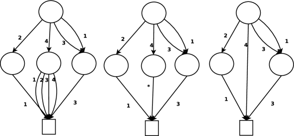
We have so far obtained a very efficient GAC algorithm for a simplified MDD data structure. In particular the algorithm described so far does not allow the MDD to be fully reduced. While simple and efficient to use, the simplified MDD is not as compact as a fully reduced MDD. It is inefficient in the case where a node $u$ exists in the MDD representing a choice point that has no effect, ie all choices lead to same node $c$. Recall that in a fully reduced MDD such a node would have been removed and its parent would instead point directly to $c$ (if no parent exist, $c$ becomes the new parent and we have an implicit edge skipping layer 1 to $l(c)-1$). Such an edge that skips a layer in the MDD is called a long edge. In the extreme the difference in edge count between the simplified MDD and the fully reduced MDD can be a factor of $nd_{max}$. An alternative that is sometimes used is to introduce wildcard nodes instead of long edges. A wildcard node only have one outgoing edge, indicating that all the node’s $d_{i}$ edges point to the same end point. This can only yield a factor of $d_{max}$ reduction in edge count over the simplified MDD, but the changes required to support wild card nodes are simpler than for long edges. Figure 5 illustrates the different edge types.

Figure 5: The decision diagrams above illustrate the effect of various methods for skipping input variables. The leftmost MDD does not skip variables, the middle one uses wildcard nodes, and the rightmost uses long edges.

6.1 Handling long edges

The simplest way to support long edges is to simply expand them for the purpose of building support lists. However, this means we use time in the total length of all the long edges, so we can no longer provide a complexity bound linear in the number of edges over a root-to-leaf path in the search tree. In the scan approach the issue of long edges is solved by scanning the BDD and for each level finding the longest outgoing edge. Given this information it is simple to list the variables which have full support due to a long edge in time $O(n)$ [12].

In our dynamic approach we do not wish to scan the MDD in order to find the longest edges. Instead, for each distinct interval supported by at least one long edge, we store the counter $L_{i,j}$, being the size of the set of long edges skipping the layers $i$ to $j$.

We will maintain the set $\mathcal{L}$ of these intervals during the search and based on these decide which variables are supported by long edges. A long edge $e$ dies if its end node $d(e)$ dies or if the assignment $(x_{s(e)},v(e))$ becomes invalid. Note that we ignore the case where a long edges dies by having all values for one of its skipped variables removed. This is safe because in this case the constraint fails. This also means we do not keep track of how many values are actually available for each skipped variable or modify the intervals if a Remove call actually ’cuts’ a long edge into two parts. This means that we allow the intervals to support values that are invalid. However, the only invalid values covered in this way are those that have explicitly been removed by calls to Remove so we can easily correct this by modifying Remove to eliminate the domain values corresponding to its arguments as we only perform decremental updates to the domains after that.

Each long edge $e$ skipping the layers from $i$ to $j$ stores a pointer to $L_{i,j}$ and when $e$ dies we decrement $L_{i,j}$. When the counter for an interval reaches zero, the interval is no longer supported by any long edge and is therefore removed from $\mathcal{L}$. We can easily create a dynamic version of the technique applied to the scanning approach for BDDs in order to handle long edges in [12]. Recall that in this case a table listing the longest outgoing edges originating from each layer is computed, and based on this the variables covered by long edges can be computed in time $O(n)$. We can obtain a dynamic version of this solution approach by store a priority queue for each level, storing the longest interval starting at that layer. Assuming the priority queue supports reporting the maximum in time $O(1)$ we can obtain the required table in $O(n)$ time as long as the priority queues are properly maintained which is done in the same manner as in the previously described approach. The following lemma gives the amortized complexity of this algorithm.

Lemma 9.

On a root-to-leaf in the search tree the complexity of the longest-outgoing-edge based approach is bounded by $O(|E|+n^{2}\lg\lg n+n^{2}d_{max})$.

Proof.

As previously, the actual time for handling normal edges is at most $O(|E|)$. Each interval can only be removed once, and each such deletion costs $O(\lg\lg|\mathcal{L}|)$ using a VEB-based priority queue[25]. Finally we spent $O(n)$ time per step to compute the table of longest outgoing edges and compute the variables covered by long edges. In total this yields a complexity over a root-to-leaf path in the search tree of $O(|E|+|\mathcal{L}|\lg\lg|\mathcal{L}|+tn)$, where $t$ is the number of steps. Since there can at most be $O(n^{2})$ distinct long edge intervals and $nd_{max}$ steps this yields $O(|E|+n^{2}\lg\lg n+n^{2}d_{max})$. ∎

As an alternative solution we can use the dynamic interval union data structure (DIU) presented in [10] to store the intervals. The DIU allows us to add or remove intervals in time $O(\lg|\mathcal{L}|)$ while allowing enumeration of the $k$ disjoint intervals representing the union of the stored intervals in time $O(k)$. Furthermore the list of values lost from the domain can be computed during a delete using just the time to enumerate them. This approach yields the following result.

Lemma 10.

On a root-to-leaf in the search tree the complexity of the DIU based approach is bounded by $O(|E|+n^{2}\lg n+nd_{max})$.

Proof.

As previously the time spent on deleting edges and handling normal edges is at most $O(|E|)$. Each interval can only be removed once and each such removal takes time at most $O(\lg|\mathcal{L}|)$. The only other work performed is to record the value removed in each step, failing the constraint if needed, costing $O(1)$ per step. This leads to a complexity of $O(|E|+|\mathcal{L}|\lg|\mathcal{L}|+t)$. Since there can at most be $O(n^{2})$ distinct long edge intervals and $nd_{max}$ steps we obtain $O(|E|+n^{2}\lg n+nd_{max})$. ∎

We believe that for most practical applications of the MDD constraint the above complexity will be completely dominated by the $|E|$ factor, and hence that the addition of long edges result in no significant performance impact. The DIU approach is most likely preferable to the longest-outgoing-edges approach in practice unless $n$ is very large and the domains very small, but replacing the VEB with a standard binary heap yields a very simple approach with a decent asymptotic complexity and good practical performance.

6.2 Handling wild card nodes

Instead of removing the nodes in a long edge, we can replace each of them with a wild card node. A wild card node has a single edge labelled $*_{i}$ representing all the outgoing edges. An interesting point about such an edge, is that during calls to Remove or RemoveScan the meaning of what allowed values it corresponds to may change, but it will change to the same for all edges labelled with $*_{i}$. Therefore, we never need to update the outgoing edge of a wildcard node, just as we didn’t update long edges. When the scanning approach is used and we encounter a wild card node $u$ which points to a live node, we can add all values in $D_{l(u)}$ to the valid domains.

When using the dynamic approach the wild card edges are not represented in the support lists. Instead a separate table containing a count of wild card nodes $w_{i}$ for each level is stored along with a list of domain values $s^{w}_{i}$ that can only be supported by wild card nodes. When a wild card node $u$ dies, $w_{i}$ is decremented, should this yield $w_{i}=0$, the values in $s^{w}_{i}$ are removed from $D_{i}$. Finally, when an assignment $(x_{i},v)$ loses support in the support list, RemoveEdge now only removes $v$ from $D_{i}$ if $w_{i}=0$ and adds $v$ to $s^{w}_{i}$ otherwise.

7 Maintaining the reduced property

In the above as well as in [9] we do not take steps to maintain the uniqueness reduced property of the MDD when we update the data structure. This forfeits a chance for a large speed-up. If a reduction at an early search node $s$ would lead to large reduction in the size of the data structure all descendant search node of $s$ (of which there can be an exponential number) would benefit from working on a much smaller data structure. An example showing the effect of dynamic reduction is given in Example 11.

Example 11.

As an example of the effect of dynamic reduction consider the simple constraint encoding the rule $x_{1}\leq x_{2},x_{1}\leq x_{3}\ldots,x_{1}\leq x_{j}$ with domains $D_{i}=\{1,\ldots,k\}$ for some constant $k$. Let $f_{v}$ denote the sub-structure representing the constraint restricted to $x_{1}=v$. Now consider the removal of the value $1$ from the domain of variable $x_{2},\ldots,x_{j}$ (as could be induced by an external AllDifferent constraint). With this restriction $f_{1}$ becomes equivalent to $f_{2}$ and can be merged, reducing the size of the MDD with a constant factor. If the value $2$ is lost next then a further constant fraction of the MDD can be removed due to the reduce step as $f_{1}=f_{2}$ now becomes equivalent to $f_{3}$. This is of course a very simplistic constraint easily propagated using other methods, but if we consider the conjunction of the constraint with another constraint, the example still applies in many cases, especially if the new constraint does not depend on the value of $x_{1}$. One example of such an additional constraint is $\forall i\in[2,j-1]:x_{i}\not=x_{i+1}$.

As we will see below, the scanning approach can be easily adapted to perform reductions, though $\Delta$-cutoff loses its benefits. The dynamic approach incurs a small performance penalty, but still elegantly avoids falling back on a scanning approach. Note that if we ensure the uniqueness reduced property the MDD will be fully reduced according to the original domains throughout the search (assuming it is fully reduced initially), since there is no risk of new long edges when we only perform domain restrictions. We therefore first discuss how to ensure the uniqueness reduced property and in section 7.3 describe the addition necessary in order to obtain full reduction according to the current domains. In section 7.4 we cover domain entailment detection for fully reduced and uniqueness reduced MDDs.

7.1 Static reduction

Our goal is to provide reduction along with our dynamic generalized arc consistency algorithm. However we will first cover how to reduce the MDD statically, such as could be done in conjunction with RemoveScan. To that end we make the following observation:

A node $u_{1}$ in layer $i$ can become redundant iff the death or merger of one or more of its children renders its live outgoing edge-set $C_{u_{1}}$ identical to another node (assuming that the MDD is uniqueness reduced for all layers below layer $i$). In order to remove this redundancy $u_{1}$ and $u_{2}$ should merge, by letting $u_{1}$ be subsumed by the identical node $u_{2}$(in this case we say that $u_{1}$ is the subsumee and $u_{2}$ the subsumer), or vice-versa. Assume that the MDD is reduced for all layers below layer $i$. Given a node $u_{1}$ in layer $i$ which changed its outgoing edges, we merely need to check if there exists another node on level $i$ which have the exact same set of children. If such a node $u_{2}$ is found, $u_{2}$ subsumes $u_{1}$ by redirecting all incoming edges that end in $u_{1}$ to $u_{2}$ and deleting all outgoing edges of $u_{1}$. Following this reduction each modified parent must be tested for redundancy. To ensure the reduced property for lower layers at all times the scan can be changed to operate in a breadth first manner, postponing all reductions until reaching the lowest layer affected by RemoveScan at which point the reductions can proceed in a bottom-up manner.

For the uniqueness test we use hashing, each node $u$ is hashed as the pair $(C_{u},l(u))$ and inserted into a hash table, updates being performed by recomputing the hash value and reinserting the node. The cost of performing the reduction during step $t$ is therefore expected $O(|E_{liv}^{t-1}|)$ assuming that universal hashing is used. The space used for the hash table is $O(|V|)$ and will therefore not have a significant impact on the total space used compared to the space needed to store the edges of the MDD.

Note that $\Delta$-cutoff is no longer useful as we have to scan the entire live part of the structure in order to ensure that its reduced.

7.2 Dynamic reduction

Let us start by considering an adaption of the static approach described above. To obtain a dynamic version we will resolve detected redundancies as above by subsuming one node into another. We can also use the same redundancy hash table. Instead of scanning for redundant nodes we simply need to check nodes that lose an outgoing edge, or have an outgoing edge redirected due to a subsume operation.

In order to make this approach correct and efficient there some issues which must be addressed. The first is to ensure that subsumptions and redundancy checks happens in the correct order. The second issue is that the process of subsuming a node can potentially be very expensive since all edges pointing to the subsumee needs to be moved. Finally we need to be able to quickly perform a redundancy check on a node, it is no longer acceptable to spent time linear in the number of outgoing edges for each such check.

7.2.1 Ordering

To ensure that nodes are considered for reduction in the correct order, we maintain a set of ’dirty’ nodes that need to be checked for redundancy. When the removal phase ends we can check these for redundancy in a bottom-up manner. Note that a redundancy check in layer $i$ can lead to a subsumption, which can lead to redundancy checks and subsumptions in layer $j<i$, but not in layer $j^{\prime}>i$. If we do not wish to reduce at every step it is safe to maintain the set of ’dirty’ nodes between steps.

7.2.2 Redundancy detection

As in the static reduction approach we will use a hash table to check for redundancy. However we need a hash value for each node that can be updated in $O(1)$ time when an outgoing edge is lost or updated. Furthermore, when inserting nodes into a hash table, it might be that other nodes have hashed to the same location, either due to a hash collision or due to the inserted node being redundant. If we do not have any efficient way to checking if it is a collision or not we will need to compare the inserted node $u_{1}$ with each of the collided nodes $u_{2}$ in turn. Such a comparison requires us to check whether $C_{u_{1}}=C_{u_{2}}$, taking time $O(\min\{|C_{u_{1}}|,C_{u_{2}}|\})$, and hence an insertion could require time $O(d_{max})$ for a constant number of collisions. We therefore require an approach that can ensure that we (almost) never need to do a full comparison with another node unless that node makes the inserted node redundant. Such an approach will ensure that insertions only take $O(1)$ time per collision. In case the inserted node is redundant we will need to perform one full comparison. To resolve such a redundancy we need to remove all edges of one of the nodes anyway, so the asymptotic complexity is not affected. For now we will assume the availability of a hashing strategy with the above properties and show what can be achieved under this assumption. Afterwards we show how to achieve such a hashing strategy in practice.

7.2.3 Merging nodes

Given two identical nodes $u_{1}$ and $u_{2}$ to merge we always designate the one with the largest number of parents as the subsumer in order to reduce the total cost of the merge operations. An edge $e$ is only moved when its end-point $c$ is subsumed. Since this only happens when another node of larger in-degree becomes identical to $c$ the in-degree required to cause $e$ to be moved must at least double each time $e$ is moved. Hence an edge can only be moved $\lceil\lg(|V|)\rceil$ times as $|V|$ is an upper bound on the in-degree of a node. Note that this is a very simple and classic greedy strategy that incurs no significant overhead.

7.2.4 Complexity of dynamic reduction

Lemma 12.

Let $m_{i}$ be the number of layer $i$ edges that are incident to a node involved in a subsumption during the part of the search corresponding to a given root-to-leaf path in the search tree. The time spent over this path by Remove on reducing the MDD is then

$$O(\lg|V|\sum_{1\leq i\leq n}m_{i})=O(|E|\lg|V|)$$

Proof.

Outgoing edges of nodes that are subsumed are simply deleted, requiring $O(1)$ time per outgoing edge. Note that each end point of the deleted edges much have an in degree of at least two before the subsumption, and therefore no further edges will need to be removed. In total this sums to $O(m_{i})$. Moving an incoming edge from the subsumee to the subsumer takes $O(1)$ time using the above mentioned hashing strategy. As demonstrated earlier, each edge will be moved at most $\lceil\lg|V|\rceil$ times. Therefore, we find that the total time spent on reducing the MDD is $O(\lg(|V|)\sum_{1\leq i\leq n}m_{i})$.

∎

Note that all of the above techniques could be applied to the scanning approach but the asymptotic performance would not change in the worst case. We also note that this dynamic approach will never use asymptotically more time on merging in total or in a single step compared to the previously described scanning approach to reduction.

7.2.5 Hashing strategy

In order to fulfill the required promises for the hashing strategy we use the following two techniques.

Fast updates

To allow quick updates of hash values we will use a slight variation on vector hashing[8, 24]. The idea behind vector hashing hashing is to hash a vector by assigning one hash function to each entry in the vector. The hash value is then computed as the XOR of each entry’s hash value. The most interesting property of vector hashing is that if a single entry changes value, the hash value can be updated in constant time, regardless of the length of the vector. In order to apply vector hashing it is necessary that each entry’s hash function is chosen from a strongly universal class of hash functions:

Definition 13 (Strongly universal hashing).

[24] A class of hash functions $\mathcal{H}\subseteq(U\rightarrow U)$ is said to be strongly universal if for all distinct $x,y\in U$ it holds that $\forall\alpha,\beta,\alpha\not=\beta:\Pr[h(x)=\alpha\land h(y)=\beta]=O(1/|U|^{2})$ for any $h$ chosen uniformly randomly from $\mathcal{H}$.

Our intention is to hash a node $u$ as a bit vector $b$ of length $d_{max}+1$ such that for $j\leq d_{max}$ the $j$th entry is the index of the node that is the end-point of the outgoing edge labelled $j$ if it exists, and $0$ otherwise. For the remaining entry we put $b_{d+1}=l(u)$, to distinguish between identical nodes in different layers. Note that this is just an encoding of $(C_{u},l(u))$ which was also used as key in Section 7.1. If we apply vector hashing directly we will need time $O(d_{l(u)})$ per node to compute the initial hash values, the total cost of which might not be bound by $O(|E|\lg|V|)$. With a slight modification presented in Lemma 14 the total time required for computing the initial hash values is reduced to $O(|E|)$.

Lemma 14.

Let $\mathcal{H}\subseteq(U\rightarrow U)$ be a class of strongly universal hash functions. Let $U_{0}$ denote a chosen ’null’ element of $U$. Define $\mathcal{H}_{U_{0}}^{S}$ as the class of hash functions $h:U^{d}\rightarrow U$ of the form $h(u)=h_{0}(U_{0})\oplus(\oplus_{u_{j}\not=U_{0}}h_{j}(u_{j}))$ where $\{h_{0},\ldots,h_{d}\}\subseteq\mathcal{H}$. Then $\mathcal{H}_{U_{0}}^{S}$ is strongly universal.

Proof.

Consider two vectors $u=(u_{1},\ldots,u_{d})$ and $q=(q_{1},\ldots,q_{d})$ such that $q\not=u$. We need to show that $\forall\alpha^{\prime},\beta^{\prime},\alpha^{\prime}\not=\beta^{\prime}:\Pr[h(q)=\alpha^{\prime}\land h(u)=\beta^{\prime}]=O(1/|U|^{2})$. We consider two cases:

Case 1

First if there is at least one entry $j$ such that $u_{j}\not=q_{j}$ and $u_{j},q_{j}\not=U_{0}$, consider fixing all hash functions except $h_{j}$. We then have $h(u)=\alpha\oplus h_{j}(u_{j})$ and $h(q)=\beta\oplus h_{j}(q_{j})$ for some fixed $\alpha$ and $\beta$.

We note that for a given choice of $\alpha,\beta,\alpha^{\prime},\beta^{\prime}$ there exists at most one pair of values for $h(u_{j})$ and $h(q_{j})$ such that $h(u)=\alpha^{\prime}\land h(q)=\beta^{\prime}$. Since $h$ is chosen from a strongly universal class of hash functions we therefore have $\Pr[h(u)=\alpha^{\prime}\land h(q)=\beta^{\prime}]=O(1/|U|^{2})$.

Case 2

If the first case does not apply then for all $1\leq k\leq d$ it is the case that either $u_{k}$ or $q_{k}$ is $U_{0}$ or $u_{k}=q_{k}$ . For this second case assume without loss of generality that $u_{j}=U_{0}\not=q_{j}$ for some $j$. We then have $h(u)=\alpha$ and $h(q)=\beta\oplus h_{j}(q_{j})$. We note that in choosing a random hash function from $\mathcal{H}_{U_{0}}^{S}$ we also choose its component hash functions independently. Therefore $h_{j}(q_{j})$ is independent from $h(u)$. Furthermore we note that for given values of $\beta$ and $\beta^{\prime}$ only one value of $h_{j}(q_{j})$ results in $h(q)=\beta^{\prime}$. Hence we obtain $\forall\alpha^{\prime},\beta^{\prime},\alpha^{\prime}\not=\beta^{\prime}:\Pr[h(u)=\alpha^{\prime}\land h(q)=\beta^{\prime}]=O(1/|U|^{2})$. ∎

To use the above result we choose a $U$ such that $V\subseteq U$ and set $U_{0}=0$. Note that the addition of $h_{0}(U_{0})$ in the lemma is only required to ensure strongly universal hashing when $U_{0}^{d}$ is allowed as key. Since this is not the case for our redundancy checks ($0^{d}$ corresponds to a dead node) $h_{0}$ is not needed.

Note that the the initial computation of the hash values during construction of the MDD now only requires $O(|E|)$ XOR operations, as the hash values only depend on existing edges. Finally, a hash value $q$ for a node $u$ can be updated in time $O(1)$ when an outgoing edge $(c,v)$ is updated to $(c^{\prime},v)$, simply by computing $q\oplus h_{v}(c)\oplus h_{v}(c^{\prime})$.

Avoiding unnecessary comparisons

So far we have not discussed an appropiate size for $U$. In practice $U$ will be chosen such that $|U|=2^{w}$ where $w$ is the word size of the relevant machine in bits. Because we use strongly universal hashing, a class of hash functions obtained by truncating the hash value to a specific length is also strongly universal[24]. Hence we can generate word size hash values and use a prefix to index the hash table. We will use the remaining bits to solve the issue of expensive collisions in the hash table, in the following way: When it becomes necessary to compare nodes within a bucket we compare the remaining bits of the hash value, and only if these are identical will we perform a full comparison of the two nodes in question.

To analyze the performance of this approach let us assume that the generated hash values contain $\lceil\lg k\rceil$ bits more than required to index the hash table, for some $k$. At any point during the search at most $|V|$ nodes are present in the hash table. In total at most $O(|E|\lg|V|)$ different nodes will be inserted during the processing of a root-to-leaf path in the search tree, since each node updates it hash value each time one of its outgoing edges is updated or removed. The expected number of elements per bucket in a hash table is $l_{b}=O(1)$. The expected number of nodes with the same full hash value is $l_{h}=O(1/k)$. Each insertion costs $O(l_{b}+d_{max}l_{h})$. Hence the expected cost of each insertion, of which there is at most $O(|E|\lg|V|)$, is $O(1+d_{max}/k)$. If $k=\Omega(d_{max})$ we obtain a total expected cost of $O(|E|\lg|V|)$ for insertions.

7.3 Full reduction based on current domains

The reduce step described above keeps the MDD fully reduced according to the original domains. This means that while the MDD is uniqueness reduced it is not fully reduced according to the current domains. As an example consider an MDD with 1 variable $x_{1}$ and a single node $u_{1}$ with edges $1$ and $2$ going to terminal. If the domain of $x_{1}$ is $\{1,2,3\}$ this MDD is fully reduced, while it reduces to the terminal node if the domain is $\{1,2\}$.

Full reduction according to the current domains can be achieved by using the following rule: If a node $u$ has live edges with labels corresponding to all values in $D_{l(u)}$ to the same child we will consider it redundant and reduce it into a long edge (or wild card node). Note that this will not result in incorrect values being added to the domains as observed in Section 6 and that this edge can only lose its supporting values if the corresponding domain is empty, in which case all the constraints fail so again we do not need to keep track of the actual ’content’ of the edge.

However, in order to maintain the MDD reduced under these new rules, we will after a domain value for $x_{i}$ is removed need to discover nodes that now support all possible values of $x_{i}$ while only having a single distinct child node.

First off we need to be able to efficiently discover that a node only has one distinct child. To this end we observe that a node either starts out with all edges pointing to the same node or achieves this status through loosing outgoing edges or having two child nodes merge to one. We can handle the second case by for each node either maintaining a unique child hash table or by using a counter in conjunction with maintaining links between edges leading to the same node.

When a node is discovered to only have one distinct child node we store them in a hash table in a way that allows us to retrieve them based on the values they support. We simply maintain a hash signature for each node on the set of labels in use on its outgoing edges, using the same variation of vector hashing used earlier, this time treating a set of value labels as a bit vector with $d_{max}$ entries. When a node is discovered to only have one distinct child node, we insert it into a hash table using the above mentioned signature. We also maintain this hash signature for each domain. When a domain value is lost, we merely update the domain signature and look up all edges corresponding exactly to the current domain (nodes having a super set of the current domain will have been discovered in an earlier step).

None of this affects the asymptotic space usage or amortized complexity of the previous reduction technique. We note that in practice we can combine the hash table needed for the uniqueness reduction and the one needed for full reduction under current domains into one in order to save space.

7.4 Domain entailment detection

Given a constraint $F_{k}$, and a partial assignment $\rho$, let $sol_{\rho}(F_{k})$ be the set of vectors of domain values corresponding to solutions allowed by this constraint that are consistent with $\rho$. A constraint $F_{k}$ is said to be domain entailed under domains $D$ iff $\times_{1\leq i\leq n}D_{i}\subseteq sol_{\rho}(F_{k})$[26]. That is, if all possible solutions to the CSP based on the available domains will be accepted by $F_{k}$ then $F_{k}$ is entailed by constraints implicit in the domains. It is beneficial to be able to detect domain entailment as it allows the solver to disregard the entailed constraint until it backtracks through the search node where the constraint was entailed.

If an MDD is kept fully reduced according to the current domains it is entirely trivial to detect domain entailment as the MDD will be reduced to the terminal node.

If the MDD is only kept uniqueness reduced and is domain entailed it is easy to see that it will consist of a path of precisely $n+1$ nodes(incl. the 1 terminal) if we use wild card nodes and a path of up to $n+1$ nodes if we use long edges. Note that this state of the MDD is both necessary and sufficient for domain entailment assuming that the MDD has performed the most recent domain propagation step. We can easily track whether or not the above properties are fulfilled using the following rules: If there is at most 1 live node per layer and the MDD constraint has not failed it is domain entailed. Naturally the node count can be maintained efficiently by simply updating a layer node counter whenever a node dies and maintaining a further counter for the number of layers having a node count of 1 or less.

8 Constructing the MDD

In order to apply our approach we first need to construct the MDD and compute the necessary auxiliary data structures.

The input to constructing the MDD is assumed to be a set of constraints expressed in discrete variable logic. For example, tabular constraints could be expressed as disjunction of tuples, while an AllDifferent would be expressed as $\forall(x_{i},x_{j})\in X^{2},i\not=j:x_{i}\not=x_{j}$.

We suggest to construct the MDD by first building the ROBDD of the component constraints using $\lg d_{i}$ binary variables to represent domain values for $x_{i}$(see for example [14]). This allows utilization of the optimized ROBDD libraries available and furthermore gives access to the many variable ordering heuristics available for BDDs which can substantially reduce the size of the BDD.

After the ROBDD is constructed it is trivial to construct the MDD from the BDD using time linear in the resulting MDD, assuming the binary variables encoding each domain variable are kept consecutive in the variable ordering. The additional data structures required by the incremental algorithm can be obtained by using the scanning approach to discover all the supporting edges.

The time that is acceptable for the compilation phase(and therefore also the allowable size of intermediate and final MDDs) depend on whether the constraint system is to be solved once or whether it is used in for example a configurator where the solver is used repeatedly on the same constraint set(with different user assignments) to compute the valid domains[23]. One could easily specify a large set of constraints and incrementally combine them into fewer and fewer MDD constraints until a time or memory limit is reached and still gain the benefit of improved propagation.

9 Other constraint compilation data structures

While we have described the above algorithms in terms of MDDs our approach also applies to similar data structures as described below.

9.1 Interval edges

In an ordinary MDD each edge corresponds to a single domain value. It is quite natural to consider the generalization to edges that represent a subset of a domain. One particular useful generalization of edges is to let each edge correspond to some interval of the domain values. This approach is used in Case DAGs[7, 11] which resemble MDDs without long edges, but where edges represent disjoint intervals instead of single values.

We could directly apply our approach above to such a Case DAG, but nodes might be stored in many more support lists than they have actual edges. This can be fixed quite easily however.

9.1.1 Basic idea

For each unique interval $I^{j}\in\mathcal{I}_{i}$ in layer $i$ we store a set $I^{j}_{E}$ of edges labelled with this interval. To each such interval we associate a counter $I^{j}_{c}$ specifying the number of valid values in the interval(so initially $I^{j}_{c}$ will simply be the size of the interval). We use $l^{I}$ to denote the sum of the size of all distinct interval present in layer $i$ and note that $l^{I}=O(nd_{max}^{3})$ since there can at most be $O(d_{i}^{2})$ distinct intervals of length at most $d_{i}$ in layer $i$.

The idea is now to maintain the set of live intervals for each layer. If we can do that efficiently we just need to be able to detect loss of domain values, which corresponds to maintaining the union of a set of intervals efficiently under deletion. Note that we do not need to split intervals when a Remove call splits the allowed domain on an edge, for similar reasons as described in Section 6.1.

This idea enables us to create a GAC that algorithm that spends time depending on the length of the distinct intervals and not on the total sum of all intervals. As comparison, the straightforward scanning approach will use time in the total interval size summed over all edges alive in the MDD in each step, meaning that processing a single edge could cost as much as $d_{max}$.

9.1.2 Maintaining the live intervals

In order to maintain the set of live intervals we need to maintain $I_{c}$ and $I_{E}$ for each interval. When performing Remove in layer $i$ we can by using an interval tree find the intervals that cover the value $v$ and decrement the corresponding counters in time $O(\lg|\mathcal{I}_{i}|+k)$ where $k$ is the number of intervals intersecting $v$. The necessity of the counter on each interval means that each interval can be accessed by by Remove as many times as the size of the interval of values it supports. RemoveEdge can work as before, the only addition being to update $I_{E}$ of the interval associated to the edge being removed.Using this approach the time for maintaining the live intervals over a search path with $t$ steps is $O(t\lg(|\mathcal{I}|)+l^{I}+|E|)=O(nd_{max}^{3}+|E|)$.

9.1.3 Maintaining the union

Since we are already spending time in the total length of the distinct intervals, we can use a very simple approach to maintain the union of the intervals. For each layer $i$ we maintain a counter indicating the number of intervals covering it. When an interval is deleted it decrements all the corresponding counters. Combined with the maintenance of the live intervals we still get a complexity of $O(nd_{max}^{3}+|E|)$. The disadvantage of this simple approach is that these relatively expensive deletions occur at lower levels in the search tree than the counter decrements. As an alternative we can use the DIU data structure described in Section 6.1 to maintain the union. Over a search path each interval can be deleted once so we get a complexity of $O(|\mathcal{I}|\lg(|\mathcal{I}|))=O(nd^{2}_{max}(\lg(n)+\lg(d_{max})))$ for handling the deletions in the DIU data structure. The reporting of values no longer covered is in total $O(nd_{max})$. Adding this to the time complexity for maintaining the live intervals we obtain a total time complexity of $O(nd^{3}_{max}+nd_{max}^{2}\lg(n)+|E|)$.

9.2 AND/OR Multi-Valued Decision Diagrams (AOMDD)

AOMDDs were introduced in [17], and from the perspective of a GAC algorithm just introduces AND nodes into the MDD, such that each child of an AND node roots an AOMDD which scope is disjoint from its siblings. This data structure is potentially much more compact than an MDD. Fortunately the above described technique can be applied easily. The only change is that an AND node dies if it looses any of its outgoing edges as opposed to all outgoing edges for an OR node. Therefore we can utilize this more compact type of decision diagram while still maintaining the complexity bounds in terms of the size of data structure.

10 Future work

One possible weakness of our approach lies in the inability to share work between multiple constraints. Just as in [9] identically structured constraints on different scopes can share the no-good cache, but that is the limit of co-operation. Specifically MDD substructure sharing between separate constraints does not extend to the support lists, while the scanning algorithm can share pruned nodes/edges and the $\Delta$-cutoff value.

Another interesting subject is the propagation between MDD constraints. Due to the size of the conjunction of a set of constraints it might be more practical to use a small set of MDD constraints each being the compilation of a subset of the original constraints. In this case it might be beneficial to consider a stronger propagation than just domain propagation among the MDD constraints. This stronger propagation could for example take the form of exchanging binary decompositions between constraints, as projections of the solution space is easy to compute in an MDD.

11 Conclusion

This paper introduced the MDD global constraint and provided an efficient incremental Generalized Arc Consistency algorithm for it based on techniques from [19], that is potentially much more efficient than the straightforward scanning approach while not using asymptotically more space. Since the constraint uses a reduced decision diagram to represent the solution space of the constraint it can be used to represent tabular constraints in a compressed manner while still allowing a complexity that relates to the size of the data structure and not the number of solutions stored as opposed to normal compression. Furthermore the MDD global constraint can be used to efficiently represent the solution space of a set of simpler constraints. As an additional advantage the constraint can be kept reduced dynamically in an efficient manner while also allowing efficient domain entailment detection. By using a good model and a good choice of global constraints, CSPs can therefore be reduced to a set of normal global constraints and a set of MDD constraints for improved domain propagation.