Functional Brain Imaging with Multi-Objective Multi-Modal Evolutionary Optimization

Abstract

Functional brain imaging is a source of spatio-temporal data mining problems. A new framework hybridizing multi-objective and multi-modal optimization is proposed to formalize these data mining problems, and addressed through Evolutionary Computation (EC).

The merits of EC for spatio-temporal data mining are demonstrated as the approach facilitates the modelling of the experts’ requirements, and flexibly accommodates their changing goals.

1 Introduction

Functional brain imaging aims at understanding the mechanisms of cognitive processes through non-invasive technologies such as magnetoencephalography (MEG). These technologies measure the surface activity of the brain with a good spatial and temporal resolution [8, 15], generating massive amounts of data.

Finding “interesting” patterns in these data, e.g. assemblies of active neuronal cells, can be viewed as a Machine Learning or a Data Mining problem. However, contrasting with ML or DM applications [6], the appropriate search criteria are not formally defined up to now; in practice the detection of active cell assemblies is manually done.

Resuming an earlier work [17], this paper formalizes functional brain imaging as a multi-objective multi-modal optimization (MoMOO) problem, and describes the evolutionary algorithm called 4D-Miner devised to tackle this problem. In this paper, the approach is extended to the search of discriminant patterns; additional criteria are devised and accommodated in order to find patterns specifically related to particular cognitive activities.

The paper is organized as follows. Section 2 introduces the background and notations; it describes the targeted spatio-temporal patterns (STP) and formalizes the MoMOO framework proposed. Section 3 describes the 4D-Miner algorithm designed for finding STPs, hybridizing multi-objective [5] and multi-modal [12] heuristics, and it reports on its experimental validation. Section 4 presents the extension of 4D-Miner to a new goal, the search for discriminant STPs. Section 5 discusses the opportunities offered by Evolutionary Data Mining, and the paper concludes with perspectives for further research.

2 Background and Notations

This section introduces the notations and criteria for Data Mining in functional brain imaging, assuming the reader’s familiarity with multi-objective optimization [5]. Let $N$ be the number of sensors and let $T$ denote the number of time steps. The $i$-th sensor is characterized by its position $M_{i}$ on the skull ($M_{i}=(x_{i},y_{i},z_{i})\in{\rm IR}^{3}$) and its activity $C_{i}(t),1\leq t\leq T$ along the experiment. Fig. 1 depicts a set of activity curves.

Figure 1: Magneto-Encephalography Data (N = 151, T = 875)

A spatio-temporal pattern noted $X=(I,i,w,r)$ is characterized from its temporal interval $I$ ($I=[t_{1},t_{2}]\subset[1,T]$) and a spatial region ${\cal B}(i,w,r)$. For the sake of convenience, spatial regions are restricted to axis-parallel ellipsoids centered on some sensor; region ${\cal B}(i,w,r)$ is the ellipsoid centered on the $i$-th sensor, which includes all sensors $j$ such that $d_{w}(M_{i},M_{j})$ is less than radius $r>0$, with

$$d_{w}(M_{i},M_{j})^{2}=w_{1}(x_{i}-x_{j})^{2}+w_{2}(y_{i}-y_{j})^{2}+w_{3}(z_{i}-z_{j})^{2}{\hskip 36.135pt}w_{1},w_{2},w_{3}>0$$

This paper focuses on the detection of assemblies of active neuronal cells, informally viewed as large spatio-temporal regions with correlated sensor activities. Formally, let $I=[t_{1},t_{2}]$ be a time interval, and let $\bar{C}_{i}^{I}$ denote the average activity of the $i$-th sensor over $I$. The $I$-alignment $\sigma_{I}(i,j)$ of sensors $i$ and $j$ over $I$ is defined as:

$$\sigma_{I}(i,j)~{}=\frac{\sum_{t=t_{1}}^{t_{2}}C_{i}(t).C_{j}(t)}{\sqrt{\sum_{t=t_{1}}^{t_{2}}C_{i}(t)^{2}}~{}\times~{}\sqrt{\sum_{t=t_{1}}^{t_{2}}C_{j}(t)^{2}}}\times\left(1-\frac{|\bar{C}_{i}^{I}-\bar{C}_{j}^{I}|}{|\bar{C}_{i}^{I}|}\right),$$

To every spatio-temporal pattern $X=(I,i,w,r)$, are thus associated i) its duration or length $\ell(X)$ ($=t_{2}-t_{1}$); ii) its area $a(X)$ (the number of sensors in ${\cal B}(i,w,r)$); and iii) its alignment $\sigma(X)$, defined as the average of $\sigma_{I}(i,j)$ for $j$ ranging in ${\cal B}(i,w,r)$. An interesting candidate pattern is one with large length, area and alignment.

Naturally, the sensor alignment tends to decrease as a longer time interval or a larger spatial region are considered, everything else being equal; conversely, the alignment increases when the duration or the area decrease. It thus comes to characterize the STP detection problem as a multi-objective optimization problem (MOO) [5], searching for large spatio-temporal regions $X$ with correlated sensor activities, i.e. patterns $X$ simultaneously maximizing criteria $\ell(X),~{}a(X)$ and $\sigma(X)$. The best compromises among these criteria, referred to as Pareto front, are the solutions of the problem.
Definition 1. (Pareto-domination)
Let $c_{1},\ldots,c_{K}$ denote $K$ criteria to be simultaneously maximized on $\Omega$. $X$ is said to Pareto-dominate $X^{\prime}$ if $X$ improves on $X^{\prime}$ with respect to all criteria, and the improvement is strict for at least one criterion. The Pareto front includes all solutions which are not Pareto-dominated.
However, the MOO setting fails to capture the true target patterns: The Pareto front defined from the above three criteria could be characterized and it does include a number of patterns; but all of these actually represent the same spatio-temporal region up to some slight variations of the time interval and the spatial region. This was found unsatisfactory as neuroscientists are actually interested in all active areas of the brain; $X$ might be worth even though its alignment, duration and area are lower than that of $X^{\prime}$, provided that $X$ and $X^{\prime}$ are situated in different regions of the brain.

The above remark leads to extend multi-objective optimization goal in the spirit of multi-modal optimization [12]. Formally, a new optimization framework is defined, referred to as multi-modal multi-objective optimization (MoMOO). MoMOO uses a relaxed inclusion relationship, noted $p$-inclusion, to relax the Pareto domination relation.
Definition 2. (p-inclusion)
Let $A$ and $B$ be two subsets of a measurable set $\Omega$, and let $p$ be a positive real number ($p\in[0,1]$). $A$ is $p$-included in $B$ iff $|A\bigcap B|>p\times|A|$, where $|A|$ denotes the measure of set $A$.
Definition 3. (multi-modal Pareto domination)
Let $X$ and $Y$ denote two spatio-temporal patterns with respective supports $Sup(X)$ and $Sup(Y)$ ($Sup(X),Sup(Y)\subset{\rm IR}^{d}$). $X$ p-mo-Pareto dominates $Y$ iff the support of $Y$ is $p$-included in that of $X$, and $X$ Pareto-dominates $Y$.
Finally, the interesting STPs are all spatio-temporal patterns which are not $p$-mo-Pareto dominated.

It must be emphasized that MoMOO differs from MOO with diversity enforcing heuristics (see e.g., [3, 11]): diversity-based heuristics in MOO aim at a better sampling of the Pareto front defined from fixed objectives; MoMOO is interested in a new Pareto front, including diversity as a new objective.

3 4D-Miner

This section describes the 4D-Miner algorithm designed for the detection of stable spatio-temporal patterns, and reports on its experimental validation.

3.1 Overview of 4D-Miner

Following [4], special care is devoted to the initialization step. In order to both favor the generation of relevant STPs and exclude the extremities of the Pareto front (patterns with insufficient alignment, or insignificant spatial or temporal amplitudes), every initial pattern $X=(i,w,I,r)$ is generated after a constrained sampling mechanism:

• Center $i$ is uniformly drawn in $[1,N]$;

• Vector $w$ is set to $(1,1,1)$ ($d_{w}$ is initialized to the Euclidean distance);

• Interval $I=[t_{1},t_{2}]$ is such that $t_{1}$ is drawn with uniform distribution in $[1,T]$; the length $t_{2}-t_{1}$ of $I_{j}$ is drawn according to a Gaussian distribution ${\cal N}(min_{\ell},min_{\ell}/10)$, where $min_{\ell}$ is a user-supplied length parameter.

• Radius $r$ is deterministically computed from a user-supplied threshold $min_{\sigma}$, corresponding to the minimal $I$-alignment desired.

  $$r=min_{k}\{d_{w}(i,k)~{}s.t.~{}\sigma_{I}(i,k)>min_{\sigma})\}$$

• Last, the spatial amplitude $a(X)$ of individual $X$ is required to be more than a user-supplied threshold $min_{a}$; otherwise, the individual is non admissible and it does not undergo mutation or crossover.

The user-supplied $min_{\ell}$, $min_{\sigma}$ and $min_{a}$ thus govern the proportion of admissible individuals in the initial population. The computational complexity of the initialization phase is ${\cal O}(P\times N\times min_{\ell})$, where $P$ is the population size, $N$ is the number of measure points and $min_{\ell}$ is the average length of the intervals.

The variation operators go as follows. From parent $X=(i,w,I,r)$, mutation generates an offspring by one among the following operators: i) replacing center $i$ with another sensor in ${\cal B}(i,w,r)$; ii) mutating $w$ and $r$ using self-adaptive Gaussian mutation; iii) incrementing or decrementing the bounds of interval $I$; iv) generating a brand new individual (using the initialization operator).
The crossover operator is subjected to restricted mating (only sufficiently close patterns are allowed to mate); it proceeds by i) swapping the centers or ii) the ellipsoid coordinates of the two individuals, or iii) merging the time intervals.

A steady state evolutionary scheme is considered. In each step, a single admissible parent individual is selected and it generates an offspring via mutation or crossover; the parent is selected using a Pareto archive-based selection [5], where the size of the Pareto archive is 10 times the population size. The offspring either replaces a non-admissible individual, or an individual selected after inverse Pareto archive-based selection.

3.2 Experimental results

This subsection reports on the experiments done using 4D-Miner on real-world datasets, collected from subjects observing a moving ball. Each dataset involves 151 measure points and the number of time steps (milliseconds) is 875. As can be noted from Fig. 1, the range of activities widely varies along time. The runtime on the available data is less than 20 seconds on PC Pentium 2.4 GHz.

The parameters used in the experiments are as follows. The population size is $P=200$; the stop criterion is based on the number of fitness evaluations per run, limited to 40,000. A few preliminary runs were used to adjust the operator rates; the mutation and crossover rates are respectively set to .7 and .3. For computational efficiency, the $p$-inclusion is computed as: $X$ is $p$-included in $Y$ if the center $i$ of $X$ belongs to the spatial support of $Y$, and there is an overlap between their time intervals. 4D-Miner is written in C⁺⁺.

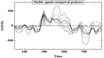
(a): $\ell(X)=8,~{}a(X)=8,~{}\sigma(X)=.29$ (b): $\ell(X)=20,~{}a(X)=9,~{}\sigma(X)=.396$

Figure 2: Two stable spatio-temporal patterns ($N=151,~{}T=875$)

Typical STPs found in the real datasets are shown in Fig. 2.(a) and (b), displaying all activity curves belonging to the STP plus the time-window of the pattern. Both patterns are considered relevant by the expert; note that the STP on the right is Pareto dominated by the one of the left.

All experiments confirm the importance of the user-defined thresholds ($min_{\ell}$, $min_{a},~{}min_{\sigma}$), defining the minimum requirements on solution individuals. Raising the thresholds beyond certain values leads to poor final results as the optimization problem becomes over constrained; lowering the thresholds leads to a crowded Pareto archive, increasing the computational time and adversely affecting the quality of the final solutions. Indeed, the coarse tuning of the parameters can be achieved based on the desired proportion of admissible individuals in the initial population. However, the fine-tuning of the parameters could not be automatized up to now, and it still requires running 4D-Miner a few times. For this reason, the control of the computational cost (through the population size and number of generations) is of utmost importance.

4 Extension to Discriminant STPs

After some active brain areas have been identified, the next task in the functional brain imaging agenda is to relate these areas to specific cognitive processes, using contrasted experimental settings. In this section, the catch versus no-catch experiment is considered; the subject sees a ball, which s/he must respectively catch (catch setting) or let go (no-catch setting). Cell assemblies that are found active in the catch setting and inactive in the no-catch one, are conjectured to relate to motor skills.

More generally, the mining task becomes to find STPs that behave differently in a pair of (positive, negative) settings, referred to as discriminant STPs. The notations are modified as follows. To the $i$-th sensor are attached its activities in the positive and negative settings, respectively noted $C_{i}^{+}(t)$ and $C_{i}^{-}(t)$; its positions are similarly noted $M_{i}^{+}$ and $M_{i}^{-}$.

The fact that the sensor position differs depending on the setting entails that the genotype of the sought patterns must be redesigned. An alternative would have been to specify the 3D coordinates of a pattern instead of centering the pattern on a sensor position. However, the spatial region of a pattern actually corresponds to a set of sensors; in other words it is a discrete entity. The use of a 3D (continuous) spatial genotype would thus require to redesign the spatial mutation operator, in order to ensure effective mutations. However, calibrating the continuous mutation operator and finding the right trade-off between ineffective and disruptive modifications of the pattern position proved to be trickier than extending the genotype.

Formally, the STP genotype noted $X(i,j,I,w,r)$ now refers to a pair of sensors $i,j$, which are closest to each other across both settings. The STP is assessed from:

• its spatial amplitude $a^{+}(X)$ (resp. $a^{-}(X)$) defined as the size of ${\cal B}^{+}(i,w,r)$, including all sensors $k$ such that $d_{w}(M^{+}_{i},M^{+}_{k})<r$ (resp. ${\cal B}^{-}(j,w,r)$, including all sensors $k$ such that $d_{w}(M^{-}_{j},M^{-}_{k})<r$)).

• its spatio-temporal alignment $\sigma^{+}(X)$ (respectively $\sigma^{-}(X)$), defined as the activity alignment of the sensors in ${\cal B}^{+}(i,w,r)$ (resp. in ${\cal B}^{-}(j,w,r)$), over time interval $I$.

The next step regards the formalization of the goal. Although neuroscientists have a clear idea of what a discriminant STP should look like, turning this idea into a set of operational requirements is by no way easy. Several formalizations were thus considered, modelling the search criteria in terms of new objectives (e.g. maximizing the difference between $\sigma^{+}$ and $\sigma^{-}$) or in terms of constraints ($|\sigma^{+}(X)-\sigma^{-}(X)|>min_{d\sigma}$). The extension of the 4D-Miner system to accommodate the new objectives and constraints was straightforward.

The visual inspection of the results found along the various modellings led the neuroscientists to introduce a new feature noted $d(X)$, the difference of the average activity in ${\cal B}^{+}(i,w,r)$ and ${\cal B}^{-}(j,w,r)$ over the time interval $I$. Finally, the search goal was modelled as an additional constraint on the STPs, expressed as $|d(X)|>min_{d}$ where $min_{d}$ is a user-supplied threshold.

Also, it was deemed neurophysiologically unlikely that a functional difference could occur in the early brain signals; only differences occurring after the motor program was completed by the subject, i.e. 200ms after the beginning of the experiment, are considered to be relevant. This requirement was expressed in a straightforward way, through a new constraint on admissible STPs, and directly at the initialization level (e.g., drawing $t_{1}$ uniformly in $[200,T]$, section 3.1).

Figs. 3.(a) and 3.(b) show two discriminant patterns, that were found to be satisfactory by the neuroscientists. Indeed, this assessment of the results pertains to the field of data mining more than discriminant learning. It is worth mentioning that the little amount of data available in this study, plus the known variability of brain activity in the general case (between different persons and for a same person at different moments, see e.g. [10]), does not permit to assess discriminant patterns (e.g. by splitting the data into training and test datasets, and evaluating the patterns extracted from the training set onto the test set).

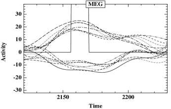
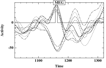
(a) (b)

Figure 3: Two discriminant stable spatio-temporal patterns. Sensors display a positive (resp. negative) activity in the catch (resp. nocatch) case. ($N=151$, $T=2500$)

Overall, the extension of 4D-Miner to the search of discriminant STPs required i) a small modification of the genotype and ii) the modelling of two additional constraints. An additional parameter was introduced, the minimum difference $min_{d}$ on the activity level, which was tuned by a few preliminary runs. Same parameters as in section 3.2 were used; the computational cost is less than 25 seconds on PC-Pentium.

5 State of the art and discussion

The presented approach is concerned with finding specific patterns in databases describing spatial objects along time.

Many approaches have been developed in signal processing and computer science to address such a goal, ranging from Fourier Transforms to Independent Component Analysis [7] and mixtures of models [2]. These approaches aim at particular pattern properties (e.g. independence, generativity) and/or focus on particular data characteristics (e.g. periodicity).

Functional brain imaging however does not fall within the range of such wide spectrum methods, for two reasons. Firstly, the sought spatio-temporal patterns are not periodic, and not independent. Secondly, and most importantly, it appears useless to build a general model of the spatio-temporal activity, while the “interesting” activity actually corresponds to a minuscule fragment of the total activity $-$ the proverbial needle in the haystack.

In the field of spatio-temporal data mining (see [18, 16] for comprehensive surveys), typical applications such as remote sensing, environmental studies, or medical imaging, involve complete algorithms, achieving an exhaustive search or building a global model. The stress is put on the scalability of the approach.

Spatio-temporal machine learning mostly focuses on clustering, outlier detection, denoising, and trend analysis. For instance, [2] used EM algorithms for non-parametric characterization of functional data (e.g. cyclone trajectories), with special care regarding the invariance of the models with respect to temporal translations. The main limitation of such non-parametric models, including Markov Random Fields, is their computational complexity; therefore the use of randomized algorithms is attracting an increasing for sidestepped by using randomized search for model estimates.

Many developments are targeted at efficient access primitives and/or complex data structures (see, e.g., [19]); another line of research is based on visual and interactive data mining (see, e.g., [9]), exploiting the unrivaled capacities of human eyes for spotting regularities in 2D-data.

More generally, the presented approach can be discussed with respect to the generative versus discriminative dilemma in Machine Learning. Although the learning goal is most often one of discrimination, generative models often outperform discriminative approaches, particularly when considering low-level information, e.g. signals, images or videos (see e.g. [14]). The higher efficiency of generative models is frequently explained as they enable the modelling and exploitation of domain knowledge in a powerful and convenient way, ultimately reducing the search space by several orders of magnitude.

In summary, generative ML extracts faithful models of the phenomenon at hand, taking advantage of whatever prior knowledge is available; these models can be used for discriminative purposes, though discrimination is not among the primary goals of generative ML. In opposition, discriminative ML focuses on the most discriminant hypotheses in the whole search space; it does not consider the relevance of a hypothesis with respect to the background knowledge per se.

To some extent, the presented approach combines generative and discriminative ML. 4D-Miner was primarily devised with the extraction of interesting patterns in mind. The core task was to model the prior knowledge through relevance criteria, combining optimization objectives (describing the expert’s preferences) and constraints (describing what is not interesting). The extraction of discriminant patterns from the relevant ones was relatively straightforward, based on the use of additional objectives and constraints. This suggests that extracting discriminant patterns from relevant ones is much easier than searching discriminant patterns, and thereafter sorting them out to find the relevant ones.

6 Conclusion and Perspectives

This paper has proposed a stochastic approach for mining stable spatio-temporal patterns. Indeed, a very simple alternative would be to discretize the spatio-temporal domain and compute the correlation of the signals in each cell of the discretization grid. However, it is believed that the proposed approach presents several advantages compared to the brute force, discretization-based, alternative.

Firstly, 4D-Miner is a fast and frugal algorithm; its good performances and scalability have been successfully demonstrated on real-world problems and on large-sized artificial datasets [17]. Secondly, data mining applications specifically involve two key steps, exemplified in this paper: i) understanding the expert’s goals and requirements; ii) tuning the parameters involved in the specifications. With regard to both steps, the ability of Evolutionary Computation to work under bounded resources is a very significant advantage. Evolutionary algorithms intrinsically are any-time algorithms, allowing the user to check at a low cost whether the process can deliver useful results, and more generally enabling her to control the trade-off between the computational resources needed and the quality of the results.

A main perspective for further research is to equip 4D-Miner with learning abilities, facilitating the automatic acquisition of the constraints and modelling the expert’s expectations. A first step would be to automatically adjust the thresholds involved in the constraints, based on the expert’s feedback. Ultimately, the goal is to design a truly user-centered mining system, combining advanced interactive optimization [13], online learning [1] and visual data mining [9].

Acknowledgments

We heartily thank Sylvain Baillet, Cognitive Neurosciences and Brain Imaging Lab., La Piti Salp tri re and CNRS, who provided the data and the interpretation of the results. The authors gratefully acknowledge the support of the Pascal Network of Excellence (IST 2002506778).

References

- [1] N. Cesa-Bianchi, A. Conconi, and C. Gentile. On the generalization ability of on-line learning algorithms. IEEE Transactions on Information Theory, 50(9):2050–2057, 2004.
- [2] D. Chudova, S. Gaffney, E. Mjolsness, and P. Smyth. Translation-invariant mixture models for curve clustering. In Proc. of the Ninth Int. Conf. on Knowledge Discovery and Data Mining, pages 79–88. ACM, 2003.
- [3] D. Corne, J. D. Knowles, and M. J. Oates. The Pareto envelope-based selection algorithm for multi-objective optimisation. In Proc. of PPSN - VI, LNCS, pages 839–848. Springer Verlag, 2000.
- [4] J. Daida. Challenges with verification, repeatability, and meaningful comparison in genetic programming: Gibson’s magic. In Proc. of GECCO 99, pages 1069–1076. Morgan Kaufmann, 1999.
- [5] K. Deb. Multi-Objective Optimization Using Evolutionary Algorithms. John Wiley, 2001.
- [6] T. Hastie, R. Tibshirani, and J. H. Friedman. The Elements of Statistical Learning: Data Mining, Inference, and Prediction. Springer Series in Statistics, 2001.
- [7] A. Hyvarinen, J. Karhunen, and E. Oja. Independent Component Analysis. Wiley New York, 2001.
- [8] M. H m l inen, R. Hari, R. Ilmoniemi, J. Knuutila, and O. V. Lounasmaa. Magnetoencephalography: theory, instrumentation, and applications to noninvasive studies of the working human brain. Rev. Mod. Phys, 65:413–497, 1993.
- [9] D. A. Keim, J. Schneidewind, and M. Sips. Circleview: a new approach for visualizing time-related multidimensional data sets. In Proc. of Advanced Visual Interfaces, pages 179–182. ACM Press, 2004.
- [10] T. Lal. Machine Learning Methods for Brain-Computer Interfaces. PhD thesis, Max Plank Institute for Biological Cybernetics, 2005.
- [11] M. Laumanns, L. Thiele, K. Deb, and E. Zitsler. Combining convergence and diversity in evolutionary multi-objective optimization. Evolutionary Computation, 10(3):263–282, 2002.
- [12] J.-P. Li, M. E. Balazs, G. T. Parks, and P. J. Clarkson. A species conserving genetic algorithm for multimodal function optimization. Evolutionary Computation, 10(3):207–234, 2002.
- [13] X. Llorà, K. Sastry, D. E. Goldberg, A. Gupta, and L. Lakshmi. Combating user fatigue in IGAs: partial ordering, support vector machines, and synthetic fitness. In Proc. of GECCO 05, pages 1363–1370. ACM, 2005.
- [14] I. McCowan, D. Gatica-Perez, S. Bengio, G. Lathoud, M. Barnard, and D. Zhang. Automatic analysis of multimodal group actions in meetings. IEEE Trans. on Pattern Analysis and Machine Intelligence (PAMI), 27(3):305–317, 2005.
- [15] D. Pantazis, T. E. Nichols, S. Baillet, and R. Leahy. A comparison of random field theory and permutation methods for the statistical analysis of MEG data. Neuroimage, 25:355–368, 2005.
- [16] J. Roddick and M. Spiliopoulou. A survey of temporal knowledge discovery paradigms and methods. IEEE Trans. on Knowledge and Data Engineering, 14(4):750–767, 2002.
- [17] M. Sebag, N. Tarrisson, O. Teytaud, S. Baillet, and J. Lefevre. A multi-objective multi-modal optimization approach for mining stable spatio-temporal patterns. In Proc. of Int. Joint Conf. on AI, IJCAI’05, pages 859–864, 2005.
- [18] S. Shekhar, P. Zhang, Y. Huang, and R. R. Vatsavai. Spatial data mining. In H. Kargupta and A. Joshi, editors, Data Mining: Next Generation Challenges and Future Directions. AAAI/MIT Press, 2003.
- [19] K. Wu, S. Chen, and P. Yu. Interval query indexing for efficient stream processing. In ACM Conf. on Information and Knowledge Management, pages 88–97. ACM Press, 2004.