INSTITUT NATIONAL DE RECHERCHE EN INFORMATIQUE ET EN AUTOMATIQUE

A higher-order active contour model of a ‘gas of circles’ and its application to tree crown extraction
Péter Horváth — Ian H. Jermyn — Zoltan Kato — Josiane Zerubia N° ????
November 2006

Abstract: Many image processing problems involve identifying the region in the image domain occupied by a given entity in the scene. Automatic solution of these problems requires models that incorporate significant prior knowledge about the shape of the region. Many methods for including such knowledge run into difficulties when the topology of the region is unknown a priori, for example when the entity is composed of an unknown number of similar objects. Higher-order active contours (HOACs) represent one method for the modelling of non-trivial prior knowledge about shape without necessarily constraining region topology, via the inclusion of non-local interactions between region boundary points in the energy defining the model.

The case of an unknown number of circular objects arises in a number of domains, e.g. medical, biological, nanotechnological, and remote sensing imagery. Regions composed of an a priori unknown number of circles may be referred to as a ‘gas of circles’. In this report, we present a HOAC model of a ‘gas of circles’. In order to guarantee stable circles, we conduct a stability analysis via a functional Taylor expansion of the HOAC energy around a circular shape. This analysis fixes one of the model parameters in terms of the others and constrains the rest. In conjunction with a suitable likelihood energy, we apply the model to the extraction of tree crowns from aerial imagery, and show that the new model outperforms other techniques.

Key-words: tree, crown, extraction, aerial image, higher-order, active contour, gas of circles, prior, shape

Un modèle de contours actifs d’ordre supérieur d’un ‘gaz de cercles’ et son application à l’extraction des houppiers

Résumé : Plusieurs problèmes en traitement d’image demandent l’identification de la région dans le domaine de l’image qui correspond à une entité donnée dans la scène. La solution automatique de ces problèmes demande des modèles qui incorporent une connaissance a priori importante de la forme de la région. Beaucoup de méthodes pour l’inclusion d’une telle connaissance ont des difficultés quand la topologie est a priori inconnue, par exemple quand l’entité est composée d’un nombre inconnu d’objets similaires. Les contours actifs d’ordre supérieur (CAOS) sont une méthode pour la modélisation d’une connaissance a priori sur la forme non-triviale sans nécessairement contraindre la topologie de la région, via l’inclusion d’interactions non-locales entre les points du bord de la région dans l’énergie qui définie le modelé.

Le cas d’un nombre inconnu d’objets circulaires se soulève dans plusieurs domaines, e.g. l’imagerie médicale, biologique, nanotechnologique, et la télédétection. Des régions composées d’un nombre inconnu de cercles peuvent être appelées un “gaz de cercles”. Dans ce rapport, nous présentons un modelé CAOS d’un gaz de cercles. Pour garantir des cercles stables, nous faisons une analyse de stabilité via un développement de Taylor fonctionnel autour d’une forme circulaire. Cette analyse fixe un des paramètres du modèle en fonction des autres, et contraint le reste. En combinaison avec une énergie d’attache aux données appropriée, nous appliquons le modèle à l’extraction des houppiers dans des images aériennes, et montrons que sa performance est meilleure que d’autres techniques.

Mots-clés : arbre, houppier, extraction, image aérienne, ordre supérieur, contour actif, gaz de cercles, a priori, forme

1 Introduction

Forestry is a domain in which image processing and computer vision techniques can have a significant impact. Resource management and conservation, whether commercial or in the public domain, require information about the current state of a forest or plantation. Much of this information can be summarized in statistics related to the size and placement of individual tree crowns (e.g. mean crown area and diameter, density of the trees). Currently, this information is gathered using expensive field surveys and time-consuming semi-automatic procedures, with the result that partial information from a number of chosen sites frequently has to be extrapolated. An image processing method capable of automatically extracting tree crowns from high resolution aerial or satellite images (an example is shown in figure 1) and computing statistics based on the results would greatly aid this domain.

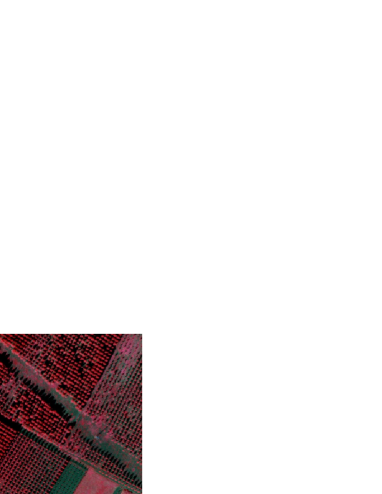
Figure 1: Real image with planted forest ©IFN.

The tree crown extraction problem can be viewed as a special case of a general image understanding problem: the identification of the region $R$ in the image domain $\Omega$ corresponding to some entity or entities in the scene. In order to solve this problem in any particular case, we have to construct, even if only implicitly, a probability distribution on the space of regions $\text{P}(R|I,K)$. This distribution depends on the current image data $I$ and on any prior knowledge $K$ we may have about the region or about its relation to the image data, as encoded in the likelihood $\text{P}(I|R,K)$ and the prior $\text{P}(R|K)$ appearing in the Bayes’ decomposition of $\text{P}(R|I,K)$ (or equivalently in their energies $-\ln\text{P}(I|R,K)$ and $-\ln\text{P}(R|K)$). This probability distribution can then be used to make estimates of the region we are looking for.

In the automatic solution of realistic problems, the prior knowledge $K$, and in particular prior knowledge about the ‘shape’ of the region, as described by $\text{P}(R|K)$, is critical. The tree crown extraction problem provides a good example: particularly in plantations, $R$ takes the form of a collection of approximately circular connected components of similar size. There is thus a great deal of prior knowledge about the region sought. The question is then how to incorporate such prior knowledge into a model for $R$? If the model does not include enough prior knowledge, it will be necessary to include it in some other form. So, for example, the use of classical active contour energies to find entities in images usually requires the initialization of the contour close to the entity to be found, which represents a large injection of prior knowledge by the user.

The simplest prior information concerns the smoothness properties of the boundary of the region. For example, the Ising model and many active contour models [18, 7, 8, 3, 4] use the length of the region boundary and its interior area as their prior energies. This type of prior information can be augmented using more demanding measures of smoothness, for example the boundary curvature [18, 14]. These models are all limited, though, by the fact that they are integrals over the region boundary of some function of various derivatives of the boundary. In consequence, they capture local differential geometric information, corresponding to local interactions between boundary points, but can say nothing more global about the shape of the region.

To go further, it is therefore clear that one must introduce longer range interactions. There are two principal ways to do this: one is to introduce hidden variables, given which the original variables of interest are (more or less) independent. Marginalizing over the hidden variables then introduces interactions between the original variables. Another is to include explicit long-range interactions between the original variables (these interactions may also have an interpretation in terms of marginalization over some hidden variables, which are left implicit).

The first approach has been much investigated, in the form of template shapes and their deformations [5, 10, 11, 9, 12, 13, 17, 22, 24, 23, 26, 21]. Here a probability distribution or an energy is defined based on a distance measure of some kind between regions. One region, the template, is fixed, while the other is the variable $R$. This type of model constrains $R$ to be close to the template region in the space of regions. Template regions may be learned from examples or fixed by hand; similarly the distance function maybe based, for example, on the learned covariance of a Gaussian distribution, or chosen a priori. The most sophisticated methods use the kernel trick to define the distance as a pullback from a high-dimensional space, thereby allowing more complex behaviours. Multiple templates may also be used, corresponding to a mixture model. It is clear that these methods implicitly introduce long-range interactions: if you know that one half of a given region aligns well with the template, this tells you something about the likely position and shape of the other half.

The above methods assign high probability to regions that lie ‘close’ to certain points in the space of regions. As such, it is difficult to construct models of this type that favour regions for which the topology, and in particular the number of connected components, is unknown a priori. There are many problems, however, for which this is the case, for example, the extraction of networks, or the extraction of an unknown number of objects of a particular type from astronomical, biological, medical, or remote sensing images. For this type of prior knowledge, a different type of model is needed. Higher-order active contours (HOACs) are one such category of models.

HOACs, first described by Rochery et al. [29] (see also [30, 31] for fuller descriptions), take the second approach mentioned above. They introduce explicit long-range interactions between region boundary points via energies that contain multiple integrals over the boundary, thus avoiding the use of template shapes. HOAC energies can be made intrinsically Euclidean invariant, and, as required by the above analysis, incorporate sophisticated prior information about region shape without necessarily constraining the topology of the region. As with other methods incorporating significant prior knowledge, it is not necessary to introduce extra knowledge via an initialization close to the target region: a generic initialization suffices, thus rendering the method quasi-automatic. Rochery et al. [29] applied the method to road extraction from satellite and aerial images using a prior which favours network-like objects.

In this report, we describe a HOAC model of a ‘gas of circles’: the model favours regions composed of an a priori unknown number of circles of a certain radius. For such a model to work, the circles must be stable to small perturbations of their boundaries, i.e. they must be local minima of the HOAC energy, for otherwise a circle would tend to ‘decay’ into other shapes. This is a non-trivial requirement. We impose it by performing a functional Taylor expansion of the HOAC energy around a circle, and then demanding that the first order term be zero for all perturbations, and that the second order term be positive semi-definite. These conditions allow us to fix one of the model parameters in terms of the others, and constrain the rest. Experiments using the HOAC energy demonstrate empirically the coherence between these theoretical considerations and the gradient descent algorithm used in practice to minimize the energy.

The model has many potential applications, to medical, biological, physical, and remote sensing imagery in which the entities to be identified are circular. We choose to apply it to the tree crown extraction problem from aerial imagery, using the ‘gas of circles’ model as a prior energy, and an appropriate likelihood. We will see that the extra prior knowledge included in the ‘gas of circles’ model permits the separation of trees that cannot be separated by simpler methods, such as maximum likelihood or classical active contours.

In the rest of this section, we present a brief introduction to HOACs. In section 2, we describe the ‘gas of circles’ HOAC model. The key to this model is the analysis of the stability of a circle as a function of the model parameters. To demonstrate the prior knowledge contained in the model, and the empirical correctness of the stability analysis, we present experimental results using the new energy. In section 3, we apply the new model to tree crown extraction. We describe a likelihood energy for trees based on the image intensity and gradient, and then present experimental results on synthetic data and on aerial images. We conclude in section 4, and discuss some open issues with the model.

1.1 Higher order active contours

As described in section 1, HOACs introduce long-range interactions between boundary points not via the intermediary of a template region or regions to which $R$ is compared, but directly, by using energy terms that involve multiple integrals over the boundary. The integrands of such integrals thus depend on two or more, perhaps widely separated, boundary points simultaneously, and can thereby impose relations between tuples of points. Euclidean invariance of such energies can be imposed directly on the energy, without the necessity to estimate a transformation between the boundary sought and the template. Perhaps more importantly, because there is no template, the topology of the region need not be constrained, a factor that is critical when the topology is not known a priori.

As with all active contour models, a region $R$ is represented by its boundary, $\partial R$. There are various ways to think of the boundary of a region. If the region has only one connected component, which is also simply-connected, then a boundary is an equivalence class of embeddings of the circle $S^{1}$ under the action of orientation-preserving diffeomorphisms of $S^{1}$. When more, possibly multiply-connected components are included, however, things get complicated. First, the number of embeddings of $S^{1}$ that are required depends on the topology, and second, there are constraints on the orientations of different components if they are to represent regions with handles.

An alternative is to view $\partial R$ as a closed $1$-chain $\gamma$ in the image domain $\Omega$ ([6] is a useful reference for the following discussion). Although region boundaries correspond to a special subset of closed $1$-chains known as domains of integration, active contour energies themselves are defined for general $1$-chains. It is convenient to use this more general context to distinguish HOAC energies from classical active contours, because it allows for notions of linearity to be used to characterize the complexity of energy functionals.

Using this representation, HOAC energies can be defined as follows [30, 31]. Let $\gamma$ be a $1$-chain in $\Omega$, and $\Box\gamma$ be its domain. Then $\gamma^{n}:(\Box\gamma)^{n}\rightarrow\Omega^{n}$ is an $n$-chain in $\Omega^{n}$. We define a class of $(n-p)$-forms on $\Omega^{n}$ that are $1$-forms with respect to $(n-p)$ factors and $0$-forms with respect to the remaining $p$ factors (by symmetry, it does not matter which $p$ factors). These forms can be pulled back to $(\Box\gamma)^{n}$ by $\gamma^{n}$. The Hodge duals of the $p$ $0$-form factors with respect to the induced metric on $\Box\gamma$ can then be taken independently on each such factor, thus converting them to $1$-forms, and rendering the whole form an $n$-form on $(\Box\gamma)^{n}$. This $n$-form can then be integrated on $(\Box\gamma)^{n}$.

In the $(n,p)=(n,0)$ cases, we are simply integrating a general $n$-form on the image of $\gamma^{n}$ in $\Omega^{n}$, thus defining a linear functional on the space of $n$-chains in $\Omega^{n}$, and hence an $n^{\text{th}}$-order monomial on the space of $1$-chains in $\Omega$. Taking arbitrary linear combinations of such monomials then gives the space of polynomial functionals on the space of $1$-chains. By analogy we refer to the general $(n,p)$ cases as ‘generalized $n^{\text{th}}$-order monomials’ on the space of $1$-chains in $\Omega$, and to arbitrary linear combinations of the latter as ‘generalized polynomial functionals’ on the space of $1$-chains in $\Omega$. HOAC energies are generalized polynomial functionals. Standard active contour energies are generalized linear functionals on $1$-chains in this sense, hence the term ‘higher-order’.

The $(1,1)$ case is simply the boundary length in some metric. An interesting application of the $(2,2)$ case to topology preservation is described by Sundaramoorthi and Yezzi [32]. The $(1,0)$ case gives the region area in some metric.

To be more concrete, we specialize to the $(n,0)$ case. Let $F$ be an $n$-form on $\Omega^{n}$. We pull $F$ back to the domain of $\gamma^{n}$ and integrate it:

$$E(\gamma)=\int_{(\partial R)^{n}}F=\int_{(\Box\gamma)^{n}}(\gamma^{n})^{\ast}F\;.$$ (1.1)

Specializing again to the case $n=2$, and using the antisymmetry of $F$ together with the symmetry of $\gamma^{2}$, we can rewrite the energy functional in this case as

$$E(\gamma)=\int_{(\partial R)^{2}}F=\int_{(\Box\gamma)^{2}}(\gamma\times\gamma)^{*}F=\iint_{(\Box\gamma)^{2}}dt\>dt^{\prime}\>\tau(t)\cdot F(\gamma(t),\gamma(t^{\prime}))\cdot\tau(t^{\prime})\;,$$ (1.2)

where $F(x,x^{\prime})$, for each $(x,x^{\prime})\in\Omega^{2}$, is a $2\times 2$ matrix, $t$ is a coordinate on $\Box\gamma$, and $\tau=\dot{\gamma}$ is the tangent vector to $\gamma$.

By imposing Euclidean invariance on this term, and adding linear terms, Rochery et al. [29] defined the following higher-order active contour prior:

$$E_{\text{g}}(\gamma)=\lambda_{C}L(\gamma)+\alpha_{C}A(\gamma)-\frac{\beta_{C}}{2}\iint dt\>dt^{\prime}\>\tau(t^{\prime})\cdot\tau(t)\>\Phi(R(t,t^{\prime}))\;,$$ (1.3)

where $L$ is the boundary length functional, $A$ is the interior area functional and $R(t,t^{\prime})=\lvert\gamma(t)-\gamma(t^{\prime})\rvert$ is the Euclidean distance between $\gamma(t)$ and $\gamma(t^{\prime})$. Rochery et al. [29] used the following interaction function $\Phi$:

$$\Phi(z)=\begin{cases}1&\text{$z<d-\epsilon$}\;,\\ \frac{1}{2}\bigl{(}1-\frac{z-d}{\epsilon}-\frac{1}{\pi}\sin\frac{\pi(z-d)}{\epsilon}\bigr{)}&\text{$d-\epsilon\leq z<d+\epsilon$}\;,\\ 0&\text{$z\geq d+\epsilon$}\;.\end{cases}$$ (1.4)

In this paper, we use this same interaction function with $d=\epsilon$, but other monotonically decreasing functions lead to qualitatively similar results.

2 The ‘gas of circles’ model

For certain ranges of the parameters involved, the energy (1.3) favours regions in the form of networks, consisting of long narrow arms with approximately parallel sides, joined together at junctions, as described by Rochery et al. [29, 30, 31]. It thus provides a good prior for network extraction from images. This behaviour does not persist for all parameter values, however, and we will exploit this parameter dependence to create a model for a ‘gas of circles’, an energy that favours regions composed of an a priori unknown number of circles of a certain radius.

For this to work, a circle of the given radius, hereafter denoted $r_{0}$, must be stable, that is, it must be a local minimum of the energy. In section 2.1, we conduct a stability analysis of a circle, and discover that stable circles are indeed possible provided certain constraints are placed on the parameters. More specifically, we expand the energy $E_{\text{g}}$ in a functional Taylor series to second order around a circle of radius $r_{0}$. The constraint that the circle be an energy extremum then requires that the first order term be zero, while the constraint that it be a minimum requires that the operator in the second order term be positive semi-definite. These requirements constrain the parameter values. In subsection 2.2, we present numerical experiments using $E_{\text{g}}$ that confirm the results of this analysis.

2.1 Stability analysis

We want to expand the energy $E_{\text{g}}$ around a circle of radius $r_{0}$. We denote a member of the equivalence class of maps representing the $1$-chain defining the circle by $\gamma_{0}$. The energy $E_{\text{g}}$ is invariant to diffeomorphisms of $\Box\gamma_{0}$, and thus is well-defined on $1$-chains. To second order,

$$E_{\text{g}}(\gamma)=E_{\text{g}}(\gamma_{0}+\delta\gamma)=E_{\text{g}}(\gamma_{0})+\langle\delta\gamma|\frac{\delta E_{\text{g}}}{\delta\gamma}\rangle_{\gamma_{0}}+\frac{1}{2}\langle\delta\gamma|\frac{\delta^{2}E_{\text{g}}}{\delta\gamma^{2}}|\delta\gamma\rangle_{\gamma_{0}}\;.$$ (2.1)

where $\langle\cdot|\cdot\rangle$ is a metric on the space of $1$-chains.

Since $\gamma_{0}$ represents a circle, it is easiest to express it in terms of polar coordinates $r,\theta$ on $\Omega$. For a suitable choice of coordinate on $S^{1}$, a circle of radius $r_{0}$ centred on the origin is then given by $\gamma_{0}(t)=(r_{0}(t),\theta_{0}(t))$, where $r_{0}(t)=r_{0}$, $\theta(t)=t$, and $t\in[-\pi,\pi)$. We are interested in the behaviour of small perturbations $\delta\gamma=(\delta r,\delta\theta)$. The first thing to notice is that because the energy $E_{\text{g}}$ is defined on $1$-chains, tangential changes in $\gamma$ do not affect its value. We can therefore set $\delta\theta=0$, and concentrate on $\delta r$.

On the circle, using the arc length parameterization $t$, the integrands of the different terms in $E_{\text{g}}$ are functions of $t-t^{\prime}$ only; they are invariant to translations around the circle. In consequence, the second derivative $\delta^{2}E_{\text{g}}/\delta\gamma(t)\delta\gamma(t^{\prime})$ is also translation invariant, and this implies that it can be diagonalized in the Fourier basis of the tangent space at $\gamma_{0}$. It thus turns out to be easiest to perform the calculation by expressing $\delta r$ in terms of this basis:

$$\delta r(t)=\sum_{k}a_{k}e^{ir_{0}kt}\;,$$ (2.2)

where $k\in\{m/r_{0}:\,m\in{\mathbb{Z}}\}$. Below, we simply state the resulting expansions to second order in the $a_{k}$ for the three terms appearing in equation (1.3). Details can be found in appendix A.

The boundary length and interior area of the region are given to second order by

$$L(\gamma) =\int_{-\pi}^{\pi}dt\>\lvert\tau(t)\rvert=2\pi r_{0}\left\{1+\frac{a_{0}}{r_{0}}+\frac{1}{2}\sum_{k}k^{2}\lvert a_{k}\rvert^{2}\right\}$$ (2.3)

$$A(\gamma) =\int_{-\pi}^{\pi}d\theta\int_{0}^{r(\theta)}dr^{\prime}\>r^{\prime}=\pi r_{0}^{2}+2\pi r_{0}a_{0}+\pi\sum_{k}\lvert a_{k}\rvert^{2}\;.$$ (2.4)

Note the $k^{2}$ in the second order term for $L$. This is the same frequency dependence as the Laplacian, and shows that the length term plays a similar smoothing role for boundary perturbations as the Laplacian does for functions. In the area term, by contrast, the Fourier perturbations are ‘white noise’.

It is also worth noting that there are no stable solutions using these terms alone. For the circle to be an extremum, we require $\lambda_{C}2\pi+\alpha_{C}2\pi r_{0}=0$, which tells us that $\alpha_{C}=-\lambda_{C}/r_{0}$. The criterion for a minimum is, for each $k$, $\lambda_{C}r_{0}k^{2}+\alpha_{C}\geq 0$. Note that we must have $\lambda_{C}>0$ for stability at high frequencies. Substituting for $\alpha_{C}$, the condition becomes $\lambda_{C}(r_{0}k^{2}-r_{0}^{-1})\geq 0$. Substituting $k=m/r_{0}$, gives the condition $m^{2}-1\geq 0$. Two points are worth noting. The first is the one we have already made: the zero frequency perturbation is not stable. The second is that the $m=1$ perturbation is marginally stable to second order, that is, such changes require no energy to this order. To fully analyse them, we must therefore go to higher order in the Taylor series. This feature will appear also in the analysis of the full energy $E_{\text{g}}$.

The quadratic term can be expressed to second order as

$$\iint_{-\pi}^{\pi}dt\>dt^{\prime}\>\tau(t^{\prime})\cdot\tau(t)\>\Phi(R(t,t^{\prime}))=2\pi\int_{-\pi}^{\pi}dp\>F_{00}(p)+4\pi a_{0}\int_{-\pi}^{\pi}dp\>F_{10}(p)\\ +\sum_{k}2\pi\lvert a_{k}\rvert^{2}\biggl{\{}\Bigl{[}2\int_{-\pi}^{\pi}dp\>F_{20}(p)+\int_{-\pi}^{\pi}dp\>e^{-ir_{0}kp}F_{21}(p)\Bigr{]}\\ -\Bigl{[}2ir_{0}k\int_{-\pi}^{\pi}dp\>e^{-ir_{0}kp}F_{23}(p)\Bigr{]}+\Bigl{[}r_{0}^{2}k^{2}\int_{-\pi}^{\pi}dp\>e^{-ir_{0}kp}F_{24}(p)\Bigr{]}\biggr{\}}\;,$$ (2.5)

The $F_{ij}$ are functionals of $\Phi$ (hence functions of $d$ and $\epsilon$ for $\Phi$ given by equation (1.4)), and functions of $r_{0}$, as well as functions of the dummy variable $p$.

Combining equations (2.3), (2.4), and (2.5), we find the energy functional (1.3) up to the second order:

$$\begin{split}E_{\text{g}}(\gamma_{0}+\delta\gamma)&=e_{0}(r_{0})+a_{0}e_{1}(r_{0})+\frac{1}{2}\sum_{k}\lvert a_{k}\rvert^{2}e_{2}(k,r_{0})\\ &=\Bigl{\{}2\pi\lambda_{C}r_{0}+\pi\alpha_{C}r_{0}^{2}-\pi\beta_{C}G_{00}(r_{0})\Bigr{\}}+a_{0}\Bigl{\{}2\pi\lambda_{C}+2\pi\alpha_{C}r_{0}-2\pi\beta_{C}G_{10}(r_{0})\Bigr{\}}\\ &+\frac{1}{2}\sum_{k}\lvert a_{k}\rvert^{2}\Bigl{\{}2\pi\lambda_{C}r_{0}k^{2}+2\pi\alpha_{C}\\ &-2\pi\beta_{C}\bigl{[}2G_{20}(r_{0})+G_{21}(k,r_{0})-2ir_{0}kG_{23}(k,r_{0})+r_{0}^{2}k^{2}G_{24}(k,r_{0})\bigr{]}\Bigr{\}}\;,\end{split}$$ (2.6)

where $G_{ij}=\int_{-\pi}^{\pi}dp\>e^{-ir_{0}(1-\delta(j))kp}F_{ij}(p)$. Note that as anticipated, there are no off-diagonal terms linking $a_{k}$ and $a_{k^{\prime}}$ for $k\neq k^{\prime}$: the Fourier basis diagonalizes the second order term.

2.1.1 Parameter constraints

Note that a circle of any radius is always an extremum for non-zero frequency perturbations ($a_{k}$ for $k\neq 0$), as these Fourier coefficients do not appear in the first order term (this is also a consequence of invariance to translations around the circle). The condition that a circle be an extremum for $a_{0}$ as well ($e_{1}=0$) gives rise to a relation between the parameters:

$$\beta_{C}(\lambda_{C},\alpha_{C},\hat{r}_{0})=\frac{\lambda_{C}+\alpha_{C}\hat{r}_{0}}{G_{10}(\hat{r}_{0})}\;,$$ (2.7)

where we have introduced $\hat{r}_{0}$ to indicate the radius at which there is an extremum, to distinguish it from $r_{0}$, the radius of the circle about which we are calculating the expansion (2.1). The left hand side of figure 2 shows a typical plot of the energy $e_{0}$ of a circle versus its radius $r_{0}$, with the $\beta_{C}$ parameter fixed using the equation (2.7) with $\lambda_{C}=1.0$, $\alpha=0.8$, and $\hat{r}_{0}=1.0$. The energy has a minimum at $r_{0}=\hat{r}_{0}$ as desired. The relationship between $\hat{r}_{0}$ and $\beta_{C}$ is not quite as straightforward as it might seem though. As can be seen, the energy also has a maximum at some radius. It is not a priori clear whether it will be the maximum or the minimum that appears at $\hat{r}_{0}$. If we graph the positions of the extrema of the energy of a circle against $\beta_{C}$ for fixed $\alpha_{C}$, we find a curve qualitatively similar to that shown in figure 3 (this is an example of a fold catastrophe). The solid curve represents the minimum, the dashed the maximum. Note that there is indeed a unique $\beta_{C}$ for a given choice of $\hat{r}_{0}$. Denote the point at the bottom of the curve by $(\beta_{C}^{(0)},\hat{r}_{0}^{(0)})$. Note that at $\beta_{C}=\beta_{C}^{(0)}$, the extrema merge and for $\beta_{C}<\beta_{C}^{(0)}$, there are no extrema: the energy curve is monotonic because the quadratic term is not strong enough to overcome the shrinking effect of the length and area terms. Note also that the minimum cannot move below $r_{0}=r_{0}^{(0)}$. This behaviour is easily understood qualitatively in terms of the interaction function in equation (1.4). If $2r_{0}<d-\epsilon$, the quadratic term will be constant, and no force will exist to stabilize the circle. In order to use equation (2.7) then, we have to ensure that we are on the upper branch of figure 3.

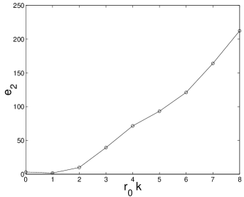
Figure 2: Plots of $e_{0}$ against $r_{0}$ and $e_{2}$ against $\hat{r}_{0}k$. Left: the energy of a circle $e_{0}$ plotted against radius $r_{0}$ for $\lambda_{C}=1.0$, $\alpha=0.8$, and $\beta_{C}=1.39$ calculated from equation (2.7) with $\hat{r}_{0}=1.0$. (The parameters of $\Phi$ are $d=1.0$ and $\epsilon=1.0$, but note that it is not necessary in general that $d=\hat{r}_{0}$.) The function has a minimum at $r_{0}=\hat{r}_{0}$ as desired. Right: the second derivative of $E_{\text{g}}$, $e_{2}$, plotted against $\hat{r}_{0}k$ for the same parameter values. The function is non-negative for all frequencies.

Equation (2.7) gives the value of $\beta_{C}$ that provides an extremum of $e_{0}$ with respect to changes of radius $a_{0}$ at a given $\hat{r}_{0}$ ($e_{1}(\hat{r}_{0})=0$), but we still need to check that the circle of radius $\hat{r}_{0}$ is indeed stable to perturbations with non-zero frequency, i.e. that $e_{2}(k,\hat{r}_{0})$ is non-negative for all $k$. Scaling arguments mean that in fact the sign of $e_{2}$ depends only on the combinations $\tilde{r}_{0}=r_{0}/d$ and $\tilde{\alpha}_{C}=(d/\lambda_{C})\alpha_{C}$. The equation for $e_{2}$ can then be used to obtain bounds on $\tilde{\alpha}_{C}$ in terms of $\tilde{r}_{0}$. (Details of these calculations and bounds will be given elsewhere.) The right hand side of figure 2 shows a plot of $e_{2}(k,\hat{r}_{0})$ against $\hat{r}_{0}k$ for the same parameter values used for the right hand side, showing that it is non-negative for all $\hat{r}_{0}k$.

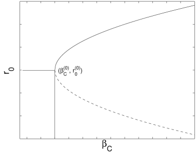
Figure 3: Schematic plot of the positions of the extrema of the energy of a circle versus $\beta_{C}$.

We call the resulting model, the energy $E_{\text{g}}$ with parameters chosen according to the above criteria, the ‘gas of circles’ model.

2.2 Geometric experiments

In order to illustrate the behaviour of the prior energy $E_{\text{g}}$ with parameter values fixed according to the above analysis, in this section we show the results of some experiments using this energy (there are no image terms). Figure 4 shows the result of gradient descent using $E_{\text{g}}$ starting from various different initial regions. (For details of the implementation of gradient descent for higher-order active contour energies using level set methods, see [30, 31].) In the first column, four different initial regions are shown. The other three columns show the final regions, at convergence, for three different sets of parameters. In particular, the three columns have $\hat{r}_{0}=15.0$, $10.0$, and $5.0$ respectively.

In the first row, the initial shape is a circle of radius $32$ pixels. The stable states, which can be seen in the other three columns, are circles with the desired radii in every case. In the second row, the initial region is composed of four circles of different radii. Depending on the value of $\hat{r}_{0}$, some of these circles shrink and disappear. This behaviour can be explained by looking at figure 2. As already noted, the energy of a circle $e_{0}$ has a maximum at some radius $r_{\text{max}}$. If an initial circle has a radius less than $r_{\text{max}}$, it will ‘slide down the energy slope’ towards $r_{0}=0$, and disappear. If its radius is larger than $r_{\text{max}}$, it will finish in the minimum, with radius $\hat{r}_{0}$. This is precisely what is observed in this second experiment. In the third row, the initial condition is composed of four squares. The squares evolve to circles of the appropriate radii. The fourth row has an initial condition composed of four differing shapes. The nature of the stable states depends on the relation between the stable radius, $\hat{r}_{0}$, and the size of the initial shapes. If $\hat{r}_{0}$ is much smaller than an initial shape, this shape will ‘decay’ into several circles of radius $\hat{r}_{0}$.

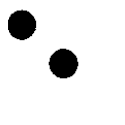
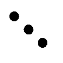
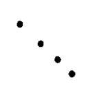
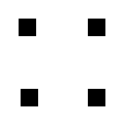
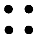
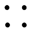
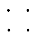
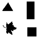
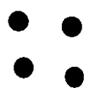
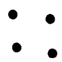
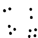
(Initial)	($\hat{r}_{0}=15$)	($\hat{r}_{0}=10$)	($\hat{r}_{0}=5$)

Figure 4: Experimental results using the geometric term: the first column shows the initial conditions; the other columns show the stable states for various choices of the radius.

3 Data terms and experiments

In this section, we apply the ‘gas of circles’ model developed in section 2 to the extraction of trees from aerial images. This is just one of many possible applications, corresponding to the mission of the Ariana research group. In the next section, we give a brief state of the art for tree crown extraction, and then present the data terms we use in section 3.2. In section 3.3, we describe tree crown extraction experiments on aerial images and compare the results to those found using a classical active contour model. In section 3.4, we examine the robustness of the method to noise using synthetic images. This illuminates the principal failure modes of the model, which will be further discussed in section 4, and which point the way for future work. In section 3.5, we illustrate the importance of prior information via tree crown separation experiments on synthetic images, and compare the results to those obtained using a classical active contour model.

3.1 Previous work

The problem of locating, counting, or delineating individual trees in high resolution aerial images has been studied in a number of papers.

Gougeon [16, 15] observes that trees are brighter than the areas separating them. Local minima of the image are found using a $3\times 3$ filter, and the ‘valleys’ connecting them are then found using a $5\times 5$ filter. The tree crowns are subsequently delineated using a five-level rule-based method designed to find circular shapes, but with some small variations permitted. Larsen [19, 20] concentrates on spruce tree detection using a template matching method. The main difference between these two papers is the use of multiple templates in the second. The 3D shape of the tree is modelled using a generalized ellipsoid, while illumination is modelled using the position of the sun and a clear-sky model. Reflectance is modelled using single reflections, with the branches and needles acting as scatterers, while the ground is treated as a Lambertian surface. Template matching is used to calculate a correlation measure between the tree image predicted by the model and the image data. The local maxima of this measure are treated as tree candidates, and various strategies are then used to eliminate false positives. Brandtberg and Walter [2] decompose an image into multiple scales, and then define tree crown boundary candidates at each scale as zero crossings with convex greyscale curvature. Edge segment centres of curvature are then used to construct a candidate tree crown region at each scale. These are then combined over different scales and a final tree crown region is grown. Andersen et al. [1] use a morphological approach combined with a top-hat transformation for the segmentation of individual trees.

All of these methods use multiple steps rather than a unified model. Closer in spirit to the present work is that of Perrin et al. [27, 28], who model the collection of tree crowns by a marked point process, where the marks are circles or ellipses. An energy is defined that penalizes, for example, overlapping shapes, and controls the parameters of the individual shapes. Reversible Jump MCMC and simulated annealing are used to estimate the tree crown configuration. Compared to the work described in this paper, the method has the advantage that overlapping trees can be represented as two separate objects, but the disadvantage that the tree crowns are not precisely delineated due to the small number of degrees of freedom for each mark.

3.2 Data terms and gradient descent

In order to couple the region model $E_{\text{g}}$ to image data, we need a likelihood, $\text{P}(I|R,K)$. The images we use for the experiments are coloured infrared (CIR) images. Originally they are composed of three bands, corresponding roughly to green, red, and near infrared (NIR). Analysis of the one-point statistics of the image in the region corresponding to trees and the image in the background, shows that the ‘colour’ information does not add a great deal of discriminating power compared to a ‘greyscale’ combination of the three bands, or indeed the NIR band on its own. We therefore model the latter.

The images have a resolution $\sim 0.5$m/pixel, and tree crowns have diameters of the order of ten pixels. Very little if any dependence remains between the pixels at this resolution, which means, when combined with the paucity of statistics within each tree crown, that pixel dependencies (i.e. texture) are very hard to use for modelling purposes. We therefore model the interior of tree crowns using a Gaussian distribution with mean $\mu$ and covariance $\sigma^{2}\delta_{R}$, where $\delta_{A}$ is the identity operator on images on $A\subset\Omega$.

The background is very varied, and thus hard to model in a precise way. We use a Gaussian distribution with mean $\bar{\mu}$ and variance $\bar{\sigma}^{2}\delta_{\bar{R}}$. In general, $\mu>\bar{\mu}$, and $\sigma<\bar{\sigma}$; trees are brighter and more constant in intensity than the background. The boundary of each tree crown has significant inward-pointing image gradient, and although the Gaussian models should in principle take care of this, we have found in practice that it is useful to add a gradient term to the likelihood energy. Our likelihood thus has three factors:

$$\text{P}(I|R,K)=Z^{-1}\>g_{R}(I_{R})\>g_{\bar{R}}(I_{\bar{R}})\>f_{\partial R}(I_{\partial R})\;.$$

where $I_{R}$ and $I_{\bar{R}}$ are the images restricted to $R$ and $\bar{R}$ respectively, and $g_{R}$ and $g_{\bar{R}}$ are proportional to the Gaussian distributions already described, i.e.

$$-\ln g_{R}(I_{R})=\int_{R}d^{2}x\>\frac{1}{2\sigma^{2}}(I_{R}(x)-\mu)^{2}$$ (3.1)

and similarly for $g_{\bar{R}}$. The function $f_{\partial R}$ depends on the gradient of the image $\partial I$ on the boundary $\partial R$:

$$-\ln f_{\partial R}(I_{\partial R})=\lambda_{i}\int_{\Box\gamma}dt\>n(t)\cdot\partial I(t)$$ (3.2)

where $n$ is the unnormalized outward normal to $\gamma$. The normalization constant $Z$ is thus a function of $\mu$, $\sigma$, $\bar{\mu}$, $\bar{\sigma}$, and $\lambda_{i}$. $Z$ is also a functional of the region $R$. To a first approximation, it is a linear combination of $L(\partial R)$ and $A(R)$. It thus has the effect of changing the parameters $\lambda_{C}$ and $\alpha_{C}$ in $E_{\text{g}}$. However, since these parameters are essentially fixed by hand (the criteria described in section 2.1.1 only allow us to fix $\beta_{C}$ and constrain $\alpha_{C}$), knowledge of the normalization constant does not change their values, and we ignore it once the likelihood parameters have been learnt.

The full model is then given by $E(R)=E_{\text{i}}(I,R)+E_{\text{g}}(R)$, where

$$E_{\text{i}}(I,R)=-\ln\text{P}(I|R,K)+\ln Z=-\ln g_{R}(I_{R})-\ln g_{\bar{R}}(I_{\bar{R}})-\ln f_{\partial R}(I_{\partial R})\;.$$

The energy is minimized by gradient descent. The gradient descent equation for $E$ is

$$\hat{n}\cdot\frac{\partial\gamma}{\partial s}(t)=-\partial^{2}I(\gamma(t))-\frac{(I(\gamma(t))-\mu)^{2}}{2\sigma^{2}}+\frac{(I(\gamma(t))-\bar{\mu})^{2}}{2\bar{\sigma}^{2}}\\ -\lambda_{C}\kappa(t)-\alpha_{C}+\beta_{C}\int_{\Box\gamma}dt^{\prime}\>\hat{R}(t,t^{\prime})\cdot n(t^{\prime})\dot{\Phi}(R(t,t^{\prime}))\;,$$ (3.3)

where $s$ is the descent time parameter, $\hat{R}(t,t^{\prime})=(\gamma(t)-\gamma(t^{\prime}))/\lvert\gamma(t)-\gamma(t^{\prime})\rvert$ and $\kappa$ is the signed boundary curvature. As already mentioned, to evolve the region we use the level set framework of Osher and Sethian [25] extended to the demands of nonlocal forces such as equation (3.3) [30, 31].

3.3 Tree crown extraction from aerial images

In this section, we present the results of the application of the above model to $50$ cm/pixel colour infrared aerial images of poplar stands located in the ‘Saône et Loire’ region in France. The images were provided by the French National Forest Inventory (IFN). As stated in section 3.2, we model only the NIR band of these images, as adding the other two bands does not increase discriminating power. The tree crowns in the images are $\sim 8$–$10$ pixels in diameter, i.e. $\sim 4$–$5$m.

In the experiments, we compare our model to a classical active contour model ($\beta_{C}=0$). The parameters $\mu$, $\sigma$, $\bar{\mu}$, and $\bar{\sigma}$ were the same for both models, and were learned from hand-labelled examples in advance. The classical active contour prior model thus has three free parameters ($\lambda_{i}$, $\lambda_{C}$ and $\alpha_{C}$), while the HOAC ‘gas of circles’ model has six ($\lambda_{i}$, $\lambda_{C}$, $\alpha_{C}$, $\beta_{C}$, $d$ and $r_{0}$). We fixed $r_{0}$ based on our prior knowledge of tree crown size in the images, and $d$ was then set equal to $r_{0}$. Once $\alpha_{C}$ and $\lambda_{C}$ have been fixed, $\beta_{C}$ is determined by equation (2.7). There are thus three effective parameters for the HOAC model. In the absence of any method to learn $\lambda_{i}$, $\alpha_{C}$ and $\lambda_{C}$, they were fixed by hand to give the best results, as with most applications of active contour models. The values of $\lambda_{i}$, $\lambda_{C}$ and $\alpha_{C}$ were not the same for the classical active contour and HOAC models; they were chosen to give the best possible result for each model separately.

The initial region in all real experiments was a rounded rectangle slightly bigger than the image domain. The image values in the region exterior to the image domain were set to $\bar{\mu}$ to ensure that the region would shrink inwards.

Figure 5 illustrates the first experiment. On the left is the data, showing a regularly planted poplar stand. The result is shown on the right. We have applied the algorithm only in the central part of the image, for reasons that will be explained in section 4.

Figure 6 illustrates a second experiment. On the left is the data. The image shows a small piece of an irregularly planted poplar forest. The image is difficult because the intensities of the crowns are varied and the gradients are blurred. In the middle is the best result we could obtain using a classical active contour. On the right is the result we obtain with the HOAC ‘gas of circles’ model. Note that in the classical active contour result several trees that are in reality separate are merged into single connected components, and the shapes of trees are often rather distorted, whereas the prior geometric knowledge included when $\beta\neq 0$ allows the separation of almost all the trees and the regularization of their shapes.

Figure 7 illustrates a third experiment. Again the data is on the left, the best result obtained with a classical active contour model is in the middle, and the result with the HOAC ‘gas of circles’ model is on the right. The trees are closer together than in the previous experiment. Using the classical active contour, the result is that the tree crown boundaries touch in the majority of cases, despite their separation in the image. Many of the connected components are malformed due to background features. The HOAC model produces more clearly delineated tree crowns, but there are still some joined trees. We will discuss this further in section 4

Figure 8 shows a fourth experiment. The data is on the left, the best result obtained with a classical active contour model is in the middle, and the result with the HOAC ‘gas of circles’ model is on the right. Again, the ‘gas of circles’ model better delineates the tree crowns and separates more trees, but some joined trees remain also. The HOAC model selects only objects of the size chosen, so that false positives involving small objects do not occur.

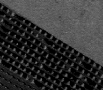
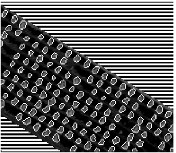
Figure 5: Left: real image with a planted forest ©IFN (0.3, 0.06, 0.05, 0.05). Right: the result obtained using the ‘gas of circles’ model $(529,5.88,5.88,5.64,4,4)$.

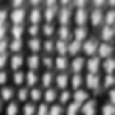
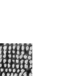
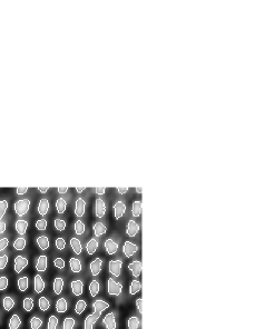
Figure 6: From left to right: image of poplars ©IFN (0.73, 0.11, 0.23, 0.094); the best result with a classical active contour $(880,13,73)$; result with the ’gas of circles’ model $(100,6.7,39,31,4.2,4.2)$.

Figure 7: From left to right: image of poplars ©IFN (0.71, 0.075, 0.18, 0.075); the best result with a classical active contour $(24000,100,500)$; result with the ’gas of circles’ model $(1500,25,130,100,3.5,3.5)$.

Figure 8: From left to right: image of poplars ©IFN (0.71, 0.075, 0.18, 0.075); the best result with a classical active contour $(35000,100,500)$; result with the ’gas of circles’ model $(1200,20,100,82,3.5,3.5)$.

Model		CAC			HOAC
Figure	CD %	FP %	FN %	CD %	F+ %	F- %
Figure 6	85	0	15	97	0	3
Figure 7	96.2	2.8	1.9	97.7	0	2.3
Figure 8	89.4	5	5.6	95.5	0.6	3.9

Table 1: Results on real images using a classical active contour model (CAC) and the ‘gas of circles’ model (HOAC). CD: correct detections; FP: false positives; FN: false negatives (two joined trees count as one false negative).

Table 1 shows the percentages of correct tree detections, false positives and false negatives (two joined trees count as one false negative), obtained with the classical active contour model and the ‘gas of circles’ model in the experiments shown in figures 6, 7, and 8. The ‘gas of circles’ model outperforms the classical active contour in all measures, except in the number of false negatives in the experiment in figure 7.

Once the segmentation result has been obtained, it is a relatively simple matter to compute statistics of interest to the forestry industry: number of trees, total area, number and area density, and so on.

3.4 Noisy synthetic images

In this section, we present the results of tests of the sensitivity of the model to noise in the image. Fifty synthetic images were created, each with ten circles with radius $8$ pixels and ten circles with radius $3.5$ pixels, placed at random but with overlaps rejected. Six different levels of white Gaussian noise, with image variance to noise power ratios from $-5$ dB to $20$ dB, were then added to the images to generate $300$ noisy images. Six of these, corresponding to noisy versions of the same original image, were used to learn $\mu$, $\sigma$, $\bar{\mu}$, and $\bar{\sigma}$. The model used was the same as that used for the aerial images, except that $\lambda_{i}$ was set equal to zero. The parameters were adjusted to give a stable radius of $8$ pixels.

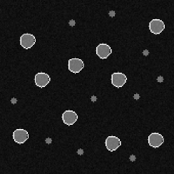
$(0.90,0.028,0.11,0.028,100,100,170)$	$(0.85,0.043,0.16,0.043,33,33,58)$
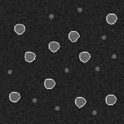
$(0.78,0.061,0.23,0.062,13,13,22)$	$(0.71,0.081,0.31,0.081,4,4,6.9)$
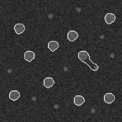
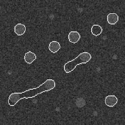
$(0.65,0.098,0.37,0.099,1.4,1.4,2.5)$	$(0.60,0.11,0.43,0.11,0.51,0.51,0.89)$

Figure 9: One of the synthesized images, with six different levels of added white Gaussian noise. Reading from left to right, top to bottom, the image variance to noise power ratios are $20$, $15$, $10$, $5$, $0$, $-5$ dB. Parameter values in the form $(\mu,\sigma,\bar{\mu},\bar{\sigma},\lambda_{C},\alpha_{C},\beta_{C})$ are shown under the six images. The parameters $d$ and $r_{0}$ were fixed to $8$ throughout.

The results obtained on the noisy versions of one of the fifty images are shown in figure 9. Table 2 shows the proportion of false negative and false positive circle detections with respect to the total number of potentially correctly detectable circles ($500=50\times 10$), as well as the proportion of ‘joined circles’, when two circles are grouped together (an example can be seen in the bottom right image of figure 9). Detections of one of the smaller circles (which only occurred a few times even at the highest noise level) were counted as false positives. The method is very robust with respect to all but the highest levels of noise. The first errors occur at $5$ dB, where there is a $2\%$ false positive rate. At $0$ dB, the error rate is $\sim 10\%$, i.e. one of the ten circles in each image was misidentified on average. At $-5$ dB, the total error rate increases to $\sim 30\%$, rendering the method not very useful.

Note that the principal error modes of the model are false positives and joined circles. There are good reasons why these two types of error dominate. We will discuss them further in section 4.

noise (dB)	FP (%)	FN (%)	J (%)
20	0	0	0
15	0	0	0
10	0	0	0
5	2	0	0
0	6.4	4	0
-5	27.6	3.6	23

Table 2: Results on synthetic noisy images. FP, FN, J: percentages of false positive, false negative, and joined circle detections respectively, with respect to the potential total number of correct detections.

3.5 Circle separation: comparison to classical active contours

In a final experiment, we simulated one of the most important causes of error in tree crown extraction, and examined the response of classical active contour and HOAC models to this situation. The errors, which involve joined circles similar to those found in the previous experiment, are caused by the fact that in many cases nearby tree crowns in an image are connected by regions of significant intensity with significant gradient with respect to the background, thus forming a dumbbell shape. Calling the bulbous extremities, the ‘bells’, and the join between them, the ‘bar’, the situation arises when the bells are brighter than the bar, while the bar is in turn brighter than the background, and most importantly, the gradient between the background and the bar is greater than that between the bar and the bells.

The first row of figure 10 shows a sequence of bells connected by bars. The intensity of the bar varies along the sequence, resulting in different gradient values. We applied the classical active contour and HOAC ‘gas of circles’ models to these images.

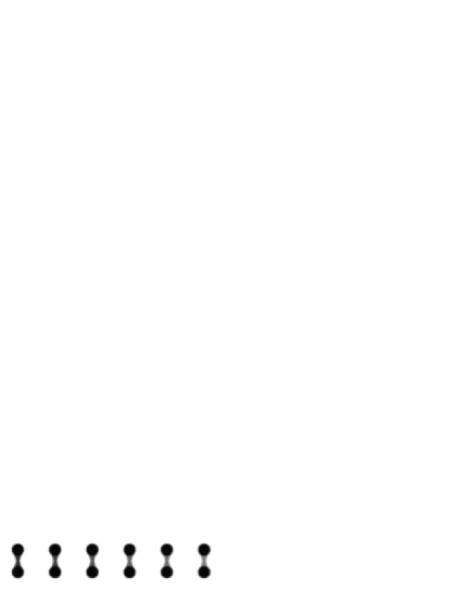
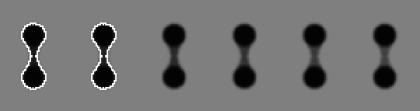
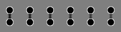
Figure 10: Results on circle separation comparing the HOAC ‘gas of circles’ model to the classical active contour model. Top: the original images. The intensity of the bar takes values equally spaced between $48$ and $128$ from left to right; the background is $255$; the bells are $0$. In the middle: the best results obtained using the classical active contour model $(8,1,1)$. Either the circles are not separated or the region vanishes. Bottom: the results using the HOAC ‘gas of circles’ model $(2,1,5,4.0,8,8)$. All the circles are segmented correctly.

The middle row of figure 10 shows the best results obtained using the classical active contour model. The model was either unable to separate the individual circles, or the region completely vanished. The intuition is that if there is insufficient gradient to stop the region at the sides of the bar, then there will also be insufficient gradient to stop the region at the boundary between the bar and the bells, so that the region will vanish. On the other hand, if there is sufficient gradient between the bar and the background to stop the region, the circles will not be separated, and a ‘bridge’ will remain between the two circles.

The corresponding results using the HOAC ‘gas of circles’ model can be seen in the bottom row of figure 10. All the circles were segmented correctly, independent of the gray level of the junction. Encouraging as this is, it is not the whole story, as we indicated in section 3.4. We make a further comment on this issue in section 4, which now follows.

4 Conclusion

Higher-order active contours allow the inclusion of sophisticated prior information in active contour models. This information can concern the relation between a region and the data, i.e. the likelihood $\text{P}(I|R,K)$, but more often it concerns the prior probability $\text{P}(R|K)$ of a region, or in other words, its ‘shape’. HOACs are particularly well adapted to including shape information about regions for which the topology is unknown a priori.

In this paper, we have shown via a stability analysis that a HOAC energy can be constructed that describes a ‘gas of circles’, that is, it favours regions composed of an a priori unknown number of circles of a certain radius, with short-range interactions amongst them. The requirement that circles be stable, i.e. local minima of the energy, fixes one of the prior parameters and constrains another.

The ‘gas of circles’ model has many potential uses in computer vision and image processing. Combined with an appropriate likelihood, we have applied it to the extraction of tree crowns from aerial images. It performs better than simpler techniques, such as maximum likelihood and standard active contours. In particular, it is better able to separate trees that appear joined in the data than a classical active contour model.

The model is not without its issues, however. The two most significant are related to the principal error modes found in the noise experiments of section 3.4: circles are found where the data does not ostensibly support them (false positives, a.k.a. ‘phantom’ circles), and two circles may be joined into a dumbbell shape and never separated. We discuss these in turn.

The first issue is that of ‘phantom’ circles. Circles of radius $\hat{r}_{0}$ are local minima of the prior energy. It is the effect of the data that converts such configurations into global minima. Were we able to find the global minimum of the energy, this would be fine. However, the fact that gradient descent finds only a local minimum can create problems in areas where the data does not support the existence of circles. This is because a circle, once formed during gradient descent, cannot disappear unless there is an image force acting on it. We thus find that circles can appear and remain even though there is no data to support them. Adding a large level of noise exacerbates this problem, because random fluctuations may encourage the appearance of circles as intermediate states during gradient descent.

The second issue is that of joined circles, discussed in section 3.5. Although the current HOAC model is better able to separate circles than a classical active contour, it still fails to do so in a number of cases, leaving a bridge between the circles. The issue here is a delicate balance between the parameters, which must be adjusted so that the sides of the bridge attract one another, thus breaking the bridge, and so that nearby circles repel one another at close range, so that the bridge does not re-form. Again, this is at least in part an algorithmic issue. Even if the two separated circles have a lower energy than the joined circles, separation may never be achieved due to a local minimum caused by the bridge. Again, high levels of noise encourage this behaviour by producing by chance image configurations that weakly support the existence of a bridge.

We are currently working on solving both these problems through a more detailed theoretical analysis of the energy, and in particular the dependence of local minima on the parameters.

Appendix A Details of stability computations

In this appendix, starting from the equation for the circle and the expression for the radial perturbation in terms of its Fourier coefficients,

$$\gamma(t) =\gamma_{0}(t)+\delta\gamma(t)=(r(t),\theta(t))=(r_{0}(t)+\delta r(t),\theta_{0}(t))$$ (A.1a)

where

$$\gamma_{0}(t) =(r_{0}(t),\theta_{0}(t))=(r_{0},t)$$ (A.1b)

and

$$\delta r(t) =\sum_{k}a_{k}e^{ir_{0}kt}\;,$$ (A.1c)

with $k\in\{m/r_{0}:\,m\in{\mathbb{Z}}\}$, we give most of the steps involved in reaching the expression, equation (2.6), for the expansion to second order of $E_{\text{g}}$ around a circle.

The derivative of $\gamma$ is given by

$$\dot{\theta}(t) =1$$ (A.2a)

$$\dot{r}(t) =\dot{\delta r}(t)=\sum_{k}a_{k}ir_{0}ke^{ir_{0}kt}\;.$$ (A.2b)

The tangent vector field is given by

$$\tau(t)=\dot{r}(t)\partial_{r}+\dot{\theta}(t)\partial_{\theta}\;.$$ (A.3)

We need the magnitude of this vector to second order. The metric in polar coordinates is given by $ds^{2}=dr^{2}+r^{2}d\theta^{2}$, so we have that $\lvert\tau(t)\rvert^{2}=\dot{r}(t)^{2}+r(t)^{2}$ by equation (A.2a). Substituting from equations (A.1) and (A.2b) gives

$$\lvert\tau(t)\rvert^{2}=r_{0}^{2}+2r_{0}\sum_{k}a_{k}e^{ir_{0}kt}+\sum_{k,k^{\prime}}a_{k}a_{k^{\prime}}e^{ir_{0}(k+k^{\prime})t}(1-r_{0}^{2}kk^{\prime})\;.$$ (A.4)

Taking the square root, expanding it as $\sqrt{1+x}\approx 1+\frac{1}{2}x-\frac{1}{8}x^{2}$, and keeping terms to second order in the $a_{k}$ then gives

$$\lvert\tau(t)\rvert=r_{0}\left\{1+\sum_{k}\frac{a_{k}}{r_{0}}e^{ir_{0}kt}-\frac{1}{2}\sum_{k,k^{\prime}}a_{k}a_{k^{\prime}}kk^{\prime}e^{ir_{0}(k+k^{\prime})t}\right\}\;.$$ (A.5)

A.1 Length

Using equation (A.5), the boundary length is then given to second order by

$$L(\gamma)=\int_{-\pi}^{\pi}dt\>\lvert\tau(t)\rvert=2\pi r_{0}\left\{1+\frac{a_{0}}{r_{0}}+\frac{1}{2}\sum_{k}k^{2}\lvert a_{k}\rvert^{2}\right\}\;,$$

where we have used the fact that

$$\int_{-\pi}^{\pi}dt\>e^{ir_{0}kt}=2\pi\delta(k)\;,$$ (A.6)

and that $a_{-k}=a_{k}^{\ast}$, where $\ast$ indicates complex conjugation, because $\delta r$ is real.

A.2 Area

We can write the interior area of the region as

$$A(\gamma)=\int_{-\pi}^{\pi}d\theta\>\int_{0}^{r(\theta)}dr^{\prime}\>r^{\prime}=\int_{-\pi}^{\pi}d\theta\>\frac{1}{2}r^{2}(\theta)\;.$$

Thus, using equations (A.1), and again using equation (A.6) to integrate Fourier basis elements, we have that

$$A(\gamma)=\pi r_{0}^{2}+2\pi r_{0}a_{0}+\pi\sum_{k}\lvert a_{k}\rvert^{2}\;.$$ (A.7)

A.3 Quadratic energy

To compute the expansion of the quadratic term in equation (1.3) for $E_{\text{g}}$, we need the expansions of $\tau(t)\cdot\tau(t^{\prime})$ and $\Phi(R(t,t^{\prime}))$.

A.3.1 Inner product of tangent vectors

The tangent vector is given by equation (A.3), but we must take care as $\tau(t)$ and $\tau(t^{\prime})$ live in different tangent spaces, at $\gamma(t)$ and $\gamma(t^{\prime})$ respectively. Since parallel transport does not preserve the coordinate basis vectors $\partial_{r}$ and $\partial_{\theta}$, it will change the components of $\tau(t^{\prime})$, say, when we parallel transport it to the tangent space at $\gamma(t)$. It is easiest to convert the tangent vectors to the Euclidean coordinate basis,

$$\partial_{r} =\cos(\theta)\partial_{x}+\sin(\theta)\partial_{y}$$

$$\partial_{\theta} =-r\sin(\theta)\partial_{x}+r\cos(\theta)\partial_{y}\;,$$

as these basis vectors are preserved by parallel transport. Doing so, and then taking the inner product gives

$$\tau\cdot\tau^{\prime}=\cos(\theta^{\prime}-\theta)[r_{0}^{2}+r_{0}\delta r+r_{0}\delta r^{\prime}+\delta r\delta r^{\prime}+\dot{\delta r}\dot{\delta r}^{\prime}]\\ +\sin(\theta^{\prime}-\theta)[r_{0}\dot{\delta r}^{\prime}-r_{0}\dot{\delta r}+\delta r\dot{\delta r}^{\prime}-\dot{\delta r}\delta r^{\prime}]\;.$$ (A.9)

where unprimed quantities are evaluated at $t$ and primed quantities at $t^{\prime}$. Note that when $t=t^{\prime}$, the expression reduces to equation (A.4).

A.3.2 Distance between two points

The squared distance between $\gamma(t^{\prime})$ and $\gamma(t)$ is given by

$$\lvert\gamma(t^{\prime})-\gamma(t)\rvert^{2} =(x(t^{\prime})-x(t))^{2}+(y(t^{\prime})-y(t))^{2}$$

$$=[(r_{0}+\delta r^{\prime})\cos(\theta^{\prime})-(r_{0}+\delta r)\cos(\theta)]^{2}+[(r_{0}+\delta r^{\prime})\sin(\theta^{\prime})-(r_{0}+\delta r)\sin(\theta)]^{2}\;,$$

which after expansion gives

$$\lvert\gamma(t^{\prime})-\gamma(t)\rvert^{2}=2r_{0}^{2}(1-\cos(\Delta t))\biggl{\{}1+\frac{1}{r_{0}}(\delta r+\delta r^{\prime})+\frac{\delta r^{2}+\delta r^{\prime 2}-2\cos(\Delta t)\delta r\delta r^{\prime}}{2r_{0}^{2}(1-\cos(\Delta t))}\biggr{\}}\;,$$

where $\Delta t=\theta^{\prime}-\theta=t^{\prime}-t$. Expanding $\sqrt{1+x}\approx 1+\frac{1}{2}x-\frac{1}{8}x^{2}$ to second order and collecting terms, we then find

$$R(t,t^{\prime})=\lvert\gamma(t^{\prime})-\gamma(t)\rvert=2r_{0}\lvert\sin(\Delta t/2)\rvert+\lvert\sin(\Delta t/2)\rvert(\delta r+\delta r^{\prime})+\frac{A(\Delta t)}{4r_{0}}(\delta r-\delta r^{\prime})^{2}\;,$$ (A.10)

where $A(z)=\left(\frac{\cos^{2}\left(\frac{z}{2}\right)}{\left|\sin\frac{z}{2}\right|}\right)$.

A.3.3 Interaction function

Expanding $\Phi(z)$ in a Taylor series to second order, and then substituting $R(t,t^{\prime})$ for $z$ using the approximation in equation (A.10), and keeping only terms up to second order in $\delta\gamma$ then gives

$$\Phi(R(t,t^{\prime}))=\Phi(X_{0})+\left\lvert\sin\frac{\Delta t}{2}\right\lvert\Phi^{\prime}(X_{0})(\delta r+\delta r^{\prime})\\ +\frac{1}{4r_{0}}A(\Delta t)\Phi^{\prime}(X_{0})(\delta r-\delta r^{\prime})^{2}+\frac{1}{2}\sin^{2}\Bigl{(}\frac{\Delta t}{2}\Bigr{)}\Phi^{\prime\prime}(X_{0})(\delta r+\delta r^{\prime})^{2}\;,$$ (A.11)

where $X_{0}=2r_{0}\lvert\sin(\Delta t/2)\rvert$.

A.3.4 Combining terms

Now let $G(t,t^{\prime})=\tau(t)\cdot\tau(t^{\prime})\Phi(R(t,t^{\prime}))$. Combining the expressions already derived, we have

$$G(t,t^{\prime})=$$

$$\underbrace{r_{0}^{2}\cos(\Delta t)\Phi(X_{0})}_{F_{00},\text{ even}}$$

$$+(\delta r+\delta r^{\prime})\underbrace{r_{0}\cos(\Delta t)\left\{\Phi(X_{0})+r_{0}\left\lvert\sin\frac{\Delta t}{2}\right\rvert\Phi^{\prime}(X_{0})\right\}}_{F_{10},\text{ even}}$$

$$+(\dot{\delta r}^{\prime}-\dot{\delta r})\underbrace{r_{0}\sin(\Delta t)\Phi(X_{0})}_{F_{11},\text{ odd}}$$

$$+(\delta r^{2}+\delta r^{\prime 2})\underbrace{r_{0}\cos(\Delta t)\left\{\frac{1}{4}A(\Delta t)\Phi^{\prime}(X_{0})+\frac{1}{2}r_{0}\sin^{2}\Bigl{(}\frac{\Delta t}{2}\Bigr{)}\Phi^{\prime\prime}(X_{0})+\left\lvert\sin\frac{\Delta t}{2}\right\lvert\Phi^{\prime}(X_{0})\right\}}_{F_{20},\text{ even}}$$

$$+(\delta r\delta r^{\prime})\underbrace{\cos(\Delta t)\left\{\Phi(X_{0})+2r_{0}\left\lvert\sin\frac{\Delta t}{2}\right\lvert\Phi^{\prime}(X_{0})-\frac{1}{2}r_{0}A(\Delta t)\Phi^{\prime}(X_{0})+r_{0}^{2}\sin^{2}\Bigl{(}\frac{\Delta t}{2}\Bigr{)}\Phi^{\prime\prime}(X_{0})\right\}}_{F_{21},\text{ even}}$$

$$+(\delta r^{\prime}\dot{\delta r}^{\prime}-\delta r\dot{\delta r})\underbrace{r_{0}\left\lvert\sin\frac{\Delta t}{2}\right\lvert\sin(\Delta t)\Phi^{\prime}(X_{0})}_{F_{22},\text{ odd}}$$

$$+(\delta r\dot{\delta r}^{\prime}-\delta r^{\prime}\dot{\delta r})\underbrace{\sin(\Delta t)\left\{\Phi(X_{0})+r_{0}\left\lvert\sin\frac{\Delta t}{2}\right\lvert\Phi^{\prime}(X_{0})\right\}}_{F_{23},\text{ odd}}$$

$$+(\dot{\delta r}\dot{\delta r}^{\prime})\underbrace{\cos(\Delta t)\Phi(X_{0})}_{F_{24},\text{ even}}\;.$$

where we have introduced the notation $F_{00}\ldots F_{24}$ for the functions appearing in the terms of $G$, and ‘odd’ and ‘even’ refer to parity under exchange of $t$ and $t^{\prime}$. Note that the $F$ are functionals of $\Phi$, and functions of $r_{0}$ and $t^{\prime}-t$ (but not $t$ and $t^{\prime}$ separately). Note also that each line, and hence $G$, is symmetric in $t$ and $t^{\prime}$.

The integral in the quadratic energy term is now given by $\iint_{-\pi}^{\pi}dt\>dt^{\prime}\>G(t,t^{\prime})$. We can now substitute the expressions for $\delta r$ and $\dot{\delta r}$ in terms of their Fourier coefficients, $\delta r(t)=\sum_{k}a_{k}e^{ir_{0}kt}$ and $\dot{\delta r}(t)=\sum_{k}a_{k}ir_{0}ke^{ir_{0}kt}$. Due to the dependence of the $F$ on $t-t^{\prime}$ only, the resulting integrals can be reduced, via a change of variables $p=t^{\prime}-t$, to integrals over $p$. We note that in the terms involving $F_{10}$, $F_{11}$, $F_{20}$, $F_{22}$, and $F_{23}$, the presence of the symmetric or antisymmetric factors in $\delta r$ and $\delta r^{\prime}$ simply leads to a doubling of the value of the integral for one of the terms in these factors, due to the corresponding symmetry or antisymmetry of the $F$ functions. For example,

$$\iint_{-\pi}^{\pi}dt\>dt^{\prime}\>(\delta r\dot{\delta r}^{\prime}-\dot{\delta r}\delta r^{\prime})\>F_{23}(t^{\prime}-t)=2\iint_{-\pi}^{\pi}dt\>dt^{\prime}\>\delta r\dot{\delta r}^{\prime}\>F_{23}(t^{\prime}-t)\;.$$

We therefore only need to evaluate one of these integrals for the relevant terms. Below we list the calculations for all the $F$ integrals for completeness:

$$\iint_{-\pi}^{\pi}dt\>dt^{\prime}\>\>F_{00}(t^{\prime}-t) =\iint_{-\pi}^{\pi}dp\>dt^{\prime}\>\>F_{00}(p)$$

$$=2\pi\int_{-\pi}^{\pi}dp\>\>F_{00}(p)\;,$$

which survives because $F_{00}$ is symmetric;

$$\iint_{-\pi}^{\pi}dt\>dt^{\prime}\>\delta r(t)\>F_{10}(t^{\prime}-t) =\iint_{-\pi}^{\pi}dt\>dt^{\prime}\>\sum_{k}a_{k}e^{ir_{0}kt}\>F_{10}(t^{\prime}-t)$$

$$=\sum_{k}a_{k}\iint_{-\pi}^{\pi}dp\>dt^{\prime}\>e^{ir_{0}k(-p+t^{\prime})}\>F_{10}(p)$$

$$=\sum_{k}a_{k}\int_{-\pi}^{\pi}dt^{\prime}\>e^{ir_{0}kt^{\prime}}\int_{-\pi}^{\pi}dp\>e^{-ir_{0}kp}\>F_{10}(p)$$

$$=\sum_{k}a_{k}2\pi\delta(k)\int_{-\pi}^{\pi}dp\>e^{-ir_{0}kp}\>F_{10}(p)$$

$$=2\pi a_{0}\int_{-\pi}^{\pi}dp\>\>F_{10}(p)\;,$$

which survives because $F_{10}$ is symmetric;

$$\iint_{-\pi}^{\pi}dt\>dt^{\prime}\>\dot{\delta r}(t)\>F_{11}(t^{\prime}-t) =\iint_{-\pi}^{\pi}dt\>dt^{\prime}\>\sum_{k}a_{k}ir_{0}ke^{ir_{0}kt}\>F_{11}(t^{\prime}-t)$$

$$=\sum_{k}a_{k}ir_{0}k\iint_{-\pi}^{\pi}dp\>dt^{\prime}\>e^{ir_{0}k(-p+t^{\prime})}\>F_{11}(p)$$

$$=\sum_{k}a_{k}ir_{0}k\int_{-\pi}^{\pi}dt^{\prime}\>e^{ir_{0}kt^{\prime}}\int_{-\pi}^{\pi}dp\>e^{-ir_{0}kp}\>F_{11}(p)$$

$$=\sum_{k}a_{k}ir_{0}k2\pi\delta(k)\int_{-\pi}^{\pi}dp\>e^{-ir_{0}kp}\>F_{11}(p)$$

$$=0\;;$$

$$\iint_{-\pi}^{\pi}dt\>dt^{\prime}\>\delta r^{2}(t)\>F_{20}(t^{\prime}-t) =\iint_{-\pi}^{\pi}dt\>dt^{\prime}\>\sum_{k}\sum_{k^{\prime}}a_{k}a_{k^{\prime}}e^{ir_{0}(k+k^{\prime})t}\>F_{20}(t^{\prime}-t)$$

$$=\sum_{k}\sum_{k^{\prime}}a_{k}a_{k^{\prime}}\iint_{-\pi}^{\pi}dp\>dt^{\prime}\>e^{ir_{0}(k+k^{\prime})(-p+t^{\prime})}\>F_{20}(p)$$

$$=\sum_{k}\sum_{k^{\prime}}a_{k}a_{k^{\prime}}\int_{-\pi}^{\pi}dt^{\prime}\>e^{ir_{0}(k+k^{\prime})t^{\prime}}\int_{-\pi}^{\pi}dp\>e^{-ir_{0}(k+k^{\prime})p}\>F_{20}(p)$$

$$=\sum_{k}\sum_{k^{\prime}}a_{k}a_{k^{\prime}}2\pi\delta(k+k^{\prime})\int_{-\pi}^{\pi}dp\>e^{-ir_{0}(k+k^{\prime})p}\>F_{20}(p)$$

$$=\sum_{k}a_{k}a_{-k}2\pi\int_{-\pi}^{\pi}dp\>F_{20}(p)$$

$$=2\pi\sum_{k}\lvert a_{k}\rvert^{2}\int_{-\pi}^{\pi}dp\>F_{20}(p)\;,$$

which survives because $F_{20}$ is symmetric;

$$\iint_{-\pi}^{\pi}dt\>dt^{\prime}\>\delta r(t)\delta r(t^{\prime})\>F_{21}(t^{\prime}-t) =\iint_{-\pi}^{\pi}dt\>dt^{\prime}\>\sum_{k}\sum_{k^{\prime}}a_{k}a_{k^{\prime}}e^{ir_{0}(kt+k^{\prime}t^{\prime})}\>F_{21}(t^{\prime}-t)$$

$$=\sum_{k}\sum_{k^{\prime}}a_{k}a_{k^{\prime}}\iint_{-\pi}^{\pi}dp\>dt^{\prime}\>e^{ir_{0}k(-p+t^{\prime})}e^{ir_{0}k^{\prime}t^{\prime}}\>F_{21}(p)$$

$$=\sum_{k}\sum_{k^{\prime}}a_{k}a_{k^{\prime}}\int_{-\pi}^{\pi}dt^{\prime}\>e^{ir_{0}(k+k^{\prime})t^{\prime}}\int_{-\pi}^{\pi}dp\>e^{-ir_{0}kp}\>F_{21}(p)$$

$$=\sum_{k}\sum_{k^{\prime}}a_{k}a_{k^{\prime}}2\pi\delta(k+k^{\prime})\int_{-\pi}^{\pi}dp\>e^{-ir_{0}kp}\>F_{21}(p)$$

$$=\sum_{k}a_{k}a_{-k}2\pi\int_{-\pi}^{\pi}dp\>e^{-ir_{0}kp}\>F_{21}(p)$$

$$=2\pi\sum_{k}\lvert a_{k}\rvert^{2}\int_{-\pi}^{\pi}dp\>e^{-ir_{0}kp}\>F_{21}(p)\;;$$

$$\iint_{-\pi}^{\pi}dt\>dt^{\prime}\>\delta r(t)\dot{\delta r}(t)\>F_{22}(t^{\prime}-t) =\iint_{-\pi}^{\pi}dt\>dt^{\prime}\>\sum_{k}\sum_{k^{\prime}}a_{k}a_{k^{\prime}}ir_{0}ke^{ir_{0}(k+k^{\prime})t}\>F_{22}(t^{\prime}-t)$$

$$=\sum_{k}\sum_{k^{\prime}}a_{k}a_{k^{\prime}}ir_{0}k\iint_{-\pi}^{\pi}dp\>dt^{\prime}\>e^{ir_{0}(k+k^{\prime})(-p+t^{\prime})}\>F_{22}(p)$$

$$=\sum_{k}\sum_{k^{\prime}}a_{k}a_{k^{\prime}}ir_{0}k\int_{-\pi}^{\pi}dt^{\prime}\>e^{ir_{0}(k+k^{\prime})t^{\prime}}\int_{-\pi}^{\pi}dp\>e^{-ir_{0}(k+k^{\prime})p}\>F_{22}(p)$$

$$=\sum_{k}\sum_{k^{\prime}}a_{k}a_{k^{\prime}}ir_{0}k2\pi\delta(k+k^{\prime})\int_{-\pi}^{\pi}dp\>e^{-ir_{0}(k+k^{\prime})p}\>F_{22}(p)$$

$$=0\;,$$

because with $k+k^{\prime}=0$ from the delta function, the integral becomes one over $F_{22}$ only, which vanishes due to the antisymmetry of $F_{22}$;

$$\iint_{-\pi}^{\pi}dt\>dt^{\prime}\>\delta r(t)\dot{\delta r}(t^{\prime})\>F_{23}(t^{\prime}-t) =\iint_{-\pi}^{\pi}dt\>dt^{\prime}\>\sum_{k}\sum_{k^{\prime}}a_{k}a_{k^{\prime}}ir_{0}k^{\prime}e^{ir_{0}(kt+k^{\prime}t^{\prime})}\>F_{23}(t^{\prime}-t)$$

$$=\sum_{k}\sum_{k^{\prime}}a_{k}a_{k^{\prime}}ir_{0}k^{\prime}\iint_{-\pi}^{\pi}dp\>dt^{\prime}\>e^{ir_{0}(k(-p+t^{\prime})+k^{\prime}t^{\prime})}\>F_{23}(p)$$

$$=\sum_{k}\sum_{k^{\prime}}a_{k}a_{k^{\prime}}ir_{0}k^{\prime}\int_{-\pi}^{\pi}dt^{\prime}\>e^{ir_{0}(k+k^{\prime})t^{\prime}}\int_{-\pi}^{\pi}dp\>e^{-ir_{0}kp}\>F_{23}(p)$$

$$=\sum_{k}\sum_{k^{\prime}}a_{k}a_{k^{\prime}}ir_{0}k^{\prime}2\pi\delta(k+k^{\prime})\int_{-\pi}^{\pi}dp\>e^{-ir_{0}kp}\>F_{23}(p)$$

$$=-2\pi\sum_{k}\lvert a_{k}\rvert^{2}ir_{0}k\int_{-\pi}^{\pi}dp\>e^{-ir_{0}kp}\>F_{23}(p)\;;$$

$$\iint_{-\pi}^{\pi}dt\>dt^{\prime}\>\dot{\delta r}(t)\dot{\delta r}(t^{\prime})\>F_{24}(t^{\prime}-t) =\iint_{-\pi}^{\pi}dt\>dt^{\prime}\>\sum_{k}\sum_{k^{\prime}}a_{k}a_{k^{\prime}}i^{2}r_{0}^{2}kk^{\prime}e^{ir_{0}(kt+k^{\prime}t^{\prime})}\>F_{24}(t^{\prime}-t)$$

$$=-\sum_{k}\sum_{k^{\prime}}a_{k}a_{k^{\prime}}r_{0}^{2}kk^{\prime}\iint_{-\pi}^{\pi}dp\>dt^{\prime}\>e^{ir_{0}(k(-p+t^{\prime})+k^{\prime}t^{\prime})}\>F_{24}(p)$$

$$=-\sum_{k}\sum_{k^{\prime}}a_{k}a_{k^{\prime}}r_{0}^{2}kk^{\prime}\int_{-\pi}^{\pi}dt^{\prime}\>e^{ir_{0}(k+k^{\prime})t^{\prime}}\int_{-\pi}^{\pi}dp\>e^{-ir_{0}kp}\>F_{24}(p)$$

$$=-\sum_{k}\sum_{k^{\prime}}a_{k}a_{k^{\prime}}r_{0}^{2}kk^{\prime}2\pi\delta(k+k^{\prime})\int_{-\pi}^{\pi}dp\>e^{-ir_{0}kp}\>F_{24}(p)$$

$$=2\pi\sum_{k}\lvert a_{k}\rvert^{2}r_{0}^{2}k^{2}\int_{-\pi}^{\pi}dp\>e^{-ir_{0}kp}\>F_{24}(p)\;.$$

Using these results then gives equation (2.5), which in combination with equations (2.3) and (2.4), gives equation (2.6).

References

- Andersen et al. [2001] H.E. Andersen, S.E. Reutebuch, and G.F. Schreuder. Automated individual tree measurement through morphological analysis of a LIDAR-based canopy surface model. In Proc. of the International Precision Forestry Symposium, pages 11–21, Seattle, Washington, USA, June 2001.
- Brandtberg and Walter [1998] T. Brandtberg and F. Walter. Automated delineation of individual tree crowns in high spatial resolution aerial images by multiple-scale analysis. Machine Vision and Applications, (2):64–73, 1998.
- Caselles et al. [1993] V. Caselles, F. Catte, T. Coll, and F. Dibos. A geometric model for active contours. Numerische Mathematik, 66:1–31, 1993.
- Caselles et al. [1997] V. Caselles, R. Kimmel, and G. Sapiro. Geodesic active contours. International Journal of Computer Vision, 22(1):61–79, 1997.
- Chen et al. [2002] Y. Chen, H.D. Tagare, S. Thiruvenkadam, F. Huang, D. Wilson, K.S. Gopinath, R.W. Briggs, and E.A. Geiser. Using prior shapes in geometric active contours in a variational framework. International Journal of Computer Vision, 50(3):315–328, 2002.
- Choquet-Bruhat et al. [1996] Y. Choquet-Bruhat, C. DeWitt-Morette, and M. Dillard-Bleick. Analysis, Manifolds and Physics. Elsevier Science, Amsterdam, The Netherlands, 1996.
- Cohen [1991] L.D. Cohen. On active contours and balloons. CVGIP: Image Understanding, 53:211–218, 1991.
- Cohen and Kimmel [1997] L.D. Cohen and R. Kimmel. Global minimum for active contour models: A minimal path approach. International Journal of Computer Vision, 24(1):57–78, August 1997.
- Cremers and Soatto [2003] D. Cremers and S. Soatto. A pseudo-distance for shape priors in level set segmentation. In Proceedings of the 2nd IEEE Workshop on Variational, Geometric and Level Set Methods, pages 169–176, Nice, France, 2003.
- Cremers et al. [2002] D. Cremers, F. Tischhäuser, J. Weickert, and C. Schnörr. Diffusion snakes: Introducing statistical shape knowledge into the Mumford-Shah functional. International Journal of Computer Vision, 50(3):295–313, 2002.
- Cremers et al. [2003] D. Cremers, T. Kohlberger, and C. Schnörr. Shape statistics in kernel space for variational image segmentation. Pattern Recognition, 36(9):1929–1943, September 2003.
- Cremers et al. [2004] D. Cremers, S. Osher, and S. Soatto. Kernel density estimation and intrinsic alignment for knowledge-driven segmentation: Teaching level sets to walk. In C. Rasmussen et al. , editor, Proc. Patt. Rec., volume 3175 of Lecture Notes in Computer Science, pages 36–44, Tübingen, Germany, 2004.
- Foulonneau et al. [2003] A. Foulonneau, P. Charbonnier, and F. Heitz. Geometric shape priors for region-based active contours. Proc. IEEE International Conference on Image Processing (ICIP), 3:413–416, 2003.
- Geman and Geman [1984] S. Geman and D. Geman. Stochastic relaxation, Gibbs distributions and the Bayesian restoration of images. IEEE Transactions on Pattern Analysis and Machine Intelligence, 6:721–741, 1984.
- Gougeon [1998] F. A. Gougeon. Automatic individual tree crown delineation using a valley-following algorithm and rule-based system. In D.A. Hill and D.G. Leckie, editors, Proc. Int’l Forum on Automated Interpretation of High Spatial Resolution Digital Imagery for Forestry, pages 11–23, Victoria, British Columbia, Canada, February 1998.
- Gougeon [1995] F.A. Gougeon. A crown-following approach to the automatic delineation of individual tree crowns in high spatial resolution aerial images. Canadian Journal of Remote Sensing, 21(3), pages 274–284, 1995.
- Grenander [1993] U. Grenander. General Pattern Theory. Oxford University Press, Oxford, UK, 1993.
- Kass et al. [1988] M. Kass, A. Witkin, and D. Terzopoulos. Snakes: Active contour models. International Journal of Computer Vision, 1(4):321–331, 1988.
- Larsen [1998] M. Larsen. Finding an optimal match window for Spruce top detection based on an optical tree model. In D.A. Hill and D.G. Leckie, editors, Proc. of the International Forum on Automated Interpretation of High Spatial Resolution Digital Imagery for Forestry, pages 55–66, Victoria, British Columbia, Canada, February 1998.
- Larsen [1999] M. Larsen. Individual Tree Top Position Estimation by Template Voting. In Proc. of the Fourth International Airborne Remote Sensing Conference and Exhibition / Canadian Symposium on Remote Sensing, volume 2, pages 83–90, Ottawa, Ontario, June 1999.
- Leventon et al. [2000] M.E. Leventon, W.E.L. Grimson, and O. Faugeras. Statistical shape influence in geodesic active contours. In Proc. IEEE Computer Vision and Pattern Recognition (CVPR), volume 1, pages 316–322, Hilton Head Island, South Carolina, USA, 2000.
- Metaxas [1997] D.N. Metaxas. Physics-based Deformable Models: Applications to Computer Vision, Graphics and Medical Imaging. Kluwer, 1997.
- Miller and Younes [2002] M. I. Miller and L. Younes. Group actions, homeomorphisms, and matching: A general framework. International Journal of Computer Vision, 41:61–84, 2002.
- Miller et al. [1997] M. I. Miller, U. Grenander, J. A. O’Sullivan, and D. L. Snyder. Automatic target recognition organized via jump-diffusion algorithms. IEEE Transactions on Image Processing, 6(1):157–174, January 1997.
- Osher and Sethian [1988] S. Osher and J. A. Sethian. Fronts propagating with curvature dependent speed: Algorithms based on Hamilton-Jacobi formulations. Journal of Computational Physics, 79(1):12–49, 1988.
- Paragios and Rousson [2002] N. Paragios and M. Rousson. Shape priors for level set representations. In Proc. European Conference on Computer Vision (ECCV), pages 78–92, Copenhagen, Denmark, 2002.
- Perrin et al. [2004] G. Perrin, X. Descombes, and J. Zerubia. Tree crown extraction using marked point processes. In Proc. European Signal Processing Conference (EUSIPCO), Vienna, Austria, September 2004.
- Perrin et al. [2005] G. Perrin, X. Descombes, and J. Zerubia. A marked point process model for tree crown extraction in plantations. In Proc. IEEE International Conference on Image Processing (ICIP), Genova, Italy, September 2005.
- Rochery et al. [2003] M. Rochery, I. H. Jermyn, and J. Zerubia. Higher order active contours and their application to the detection of line networks in satellite imagery. In Proc. IEEE Workshop Variational, Geometric and Level Set Methods in Computer Vision, at ICCV, Nice, France, October 2003.
- Rochery et al. [2005] M. Rochery, I. H. Jermyn, and J. Zerubia. Higher order active contours. Research Report 5656, INRIA, France, August 2005.
- Rochery et al. [2006] M. Rochery, I. H. Jermyn, and J. Zerubia. Higher-order active contours. International Journal of Computer Vision, 69(1):27–42, 2006. URL http://dx.doi.org/10.1007/s11263-006-6851-y.
- Sundaramoorthi and Yezzi [2005] G. Sundaramoorthi and A. Yezzi. More-than-topology-preserving flows for active contours and polygons. In Proc. IEEE International Conference on Computer Vision (ICCV), pages 1276–1283, Beijing, China, 2005.