Distributed Control of Microscopic Robots in Biomedical Applications

Abstract

Current developments in molecular electronics, motors and chemical sensors could enable constructing large numbers of devices able to sense, compute and act in micron-scale environments. Such microscopic machines, of sizes comparable to bacteria, could simultaneously monitor entire populations of cells individually in vivo. This paper reviews plausible capabilities for microscopic robots and the physical constraints due to operation in fluids at low Reynolds number, diffusion-limited sensing and thermal noise from Brownian motion. Simple distributed controls are then presented in the context of prototypical biomedical tasks, which require control decisions on millisecond time scales. The resulting behaviors illustrate trade-offs among speed, accuracy and resource use. A specific example is monitoring for patterns of chemicals in a flowing fluid released at chemically distinctive sites. Information collected from a large number of such devices allows estimating properties of cell-sized chemical sources in a macroscopic volume. The microscopic devices moving with the fluid flow in small blood vessels can detect chemicals released by tissues in response to localized injury or infection. We find the devices can readily discriminate a single cell-sized chemical source from the background chemical concentration, providing high-resolution sensing in both time and space. By contrast, such a source would be difficult to distinguish from background when diluted throughout the blood volume as obtained with a blood sample.

1 Microscopic Robots

Robots with sizes comparable to bacteria could operate in microscopic environments on the scale of individual cells in biological organisms. Such robots are small enough to move through the tiniest blood vessels, so could pass within a few cell diameters of most cells in large organisms via their circulatory systems to perform a wide variety of biological research and medical tasks. For instance, robots and nanoscale-structured materials inside the body could significantly improve disease diagnosis and treatment [16, 42, 45, 34]. Initial tasks for microscopic robots include in vitro research via simultaneous monitoring of chemical signals exchanged among many bacteria in a biofilm. The devices could also operate in multicellular organisms as passively circulating sensors. Such devices, with no need for locomotion, would detect programmed patterns of chemicals as they pass near cells. More advanced technology could create devices able to communicate to external detectors, allowing real-time in vivo monitoring of many cells. The devices could also have capabilities to act on their environment, e.g., releasing drugs at locations with specific chemical patterns or mechanically manipulating objects for microsurgery. Extensive development and testing is necessary before clinical use, first for high-resolution diagnostics and later for programmed actions at cellular scales.

Realizing these benefits requires fabricating the robots cheaply, in large numbers and with sufficient capabilities. Such fabrication is beyond current technology. Nevertheless, ongoing progress in engineering nanoscale devices could eventually enable production of such robots. One approach is engineering biological systems, e.g., bacteria executing simple programs [1], and DNA computers responding to logical combinations of chemicals [3]. However, biological organisms have limited material properties and computational speed. Instead we focus on machines based on plausible extensions of current molecular-scale electronics, sensors and motors [6, 11, 12, 30, 19, 41, 54, 59]. These devices could provide components for stronger and faster microscopic robots than is possible with biological organisms.

Because we cannot yet fabricate microscopic robots with molecular electronics components, estimates of their performance rely on plausible extrapolations from current technology. The focus in this paper is on biomedical applications requiring only modest hardware capabilities, which will be easier to fabricate than more capable robots. Designing controls for microscopic robots is a key challenge: not only enabling useful performance but also compensating for their limited computation, locomotion or communication abilities. Theoretical studies allow developing such controls and estimating their performance prior to fabrication, thereby indicating design tradeoffs among hardware capabilities, control methods and task performance. Such studies of microscopic robots complement analyses of individual nanoscale devices [40, 59], and indicate even modest capabilities enable a range of novel applications.

The operation of microscopic robots differs significantly from larger robots [38], especially for biomedical applications. First, the physical environment is dominated by viscous fluid flow. Second, thermal noise is a significant source of sensor error and Brownian motion limits the ability to follow precisely specified paths. Third, relevant objects are often recognizable via chemical signatures rather than, say, visual markings or specific shapes. Fourth, the tasks involve large numbers of robots, each with limited abilities. Moreover, a task will generally only require a modest fraction of the robots to respond appropriately, not for all, or even most, robots to do so. Thus controls using random variations are likely to be effective simply due to the large number of robots. This observation contrasts with teams of larger robots with relatively few members: incorrect behavior by even a single robot can significantly decrease team performance. These features suggest reactive distributed control is particularly well-suited for microscopic robots.

Organisms contain many microenvironments, with distinct physical, chemical and biological properties. Often, precise quantitative values of properties relevant for robot control will not be known a priori. This observation suggests a multi-stage protocol for using the robots. First, an information-gathering stage with passive robots placed into the organism, e.g., through the circulatory system, to measure relevant properties [28]. The information from these robots, in conjunction with conventional diagnostics at larger scales, could then determine appropriate controls for further actions in subsequent stages of operation.

For information gathering, each robot notes in its memory whenever chemicals matching a prespecified pattern are found. Eventually, the devices are retrieved and information in their memories extracted for further analysis in a conventional computer with far more computational resources than available to any individual microscopic robot. This computer would have access to information from many robots, allowing evaluation of aggregate properties of the population of cells that individual robots would not have access to, e.g., the number of cells presenting a specific combination of chemicals. This information allows estimating spatial structure and strength of the chemical sources. The robots could detect localized high concentrations that are too low to distinguish from background concentrations when diluted in the whole blood volume as obtained with a sample. Moreover, if the detection consists of the joint expression of several chemicals, each of which also occurs from separate sources, the robot’s pattern recognition capability could identify the spatial locality, which would not be apparent when the chemicals are mixed throughout the blood volume.

Estimating the structure of the chemical sources from the microscopic sensor data is analogous to computerized tomography [43]. In tomography, the data consists of integrals of the quantity of interest (e.g., density) over a large set of lines with known geometry selected by the experimenter. The microscopic sensors, on the other hand, record data points throughout the tissue, providing more information than just one aggregate value such as the total number of events. However, the precise path of each sensor through the tissue, i.e., which vessel branches it took and the locations of those vessels, will not be known. This mode of operation also contrasts with uses of larger distributed sensor networks able to process information and communicate results while in use.

Actions based on the information from the robots would form a second stage of activity, perhaps with specialized microscopic robots (e.g., containing drugs to deliver near cells), with controls set based on the calibration information retrieved earlier. For example, the robots could release drugs at chemically distinctive sites [16, 18] with specific detection thresholds determined with the information retrieved from the first stage of operation. Or robots could aggregate at the chemical sources [9, 26] or manipulate biological structures based on surface chemical patterns on cells, e.g., as an aid for microsurgery in repairing injured nerves [29]. These active scenarios require more advanced robot capabilities, such as locomotion and communication, than needed for passive sensing. The robots could monitor environmental changes due to their actions, thereby documenting the progress of the treatment. Thus the researcher or physician could monitor the robots’ progress and decide whether and when they should continue to the next step of the procedure. Using a series of steps, with robots continuing with the next step only when instructed by the supervising person, maintains overall control of the robots, and simplifies the control computations each robot must perform itself.

To illustrate controls for large collections of microscopic robots, this paper considers a prototypical diagnostic task of finding a small chemical source in a multicellular organism via the circulatory system. To do so, we first describe plausible capabilities for the robots and techniques for evaluating their behavior. We then examine a specific task scenario. The emphasis here is on feasible performance with plausible biophysical parameters and robot capabilities. Evaluation metrics include minimizing hardware capabilities to simplify fabrication and ensuring safety, speed and accuracy for biological research or treatment in a clinical setting.

2 Capabilities of Microscopic Robots

This section describes plausible robot capabilities based on currently demonstrated nanoscale technology. Minimal capabilities needed for biomedical tasks include chemical sensing, computation and power. Additional capabilities, enabling more sophisticated applications, include communication and locomotion.

2.1 Chemical Sensing

Large-scale robots often use sonar or cameras to sense their environment. These sensors locate objects from a distance, and involve sophisticated algorithms with extensive computational requirements. In contrast, microscopic robots for biological applications will mainly use chemical sensors, e.g., the selective binding of molecules to receptors altering the electrical characteristics of nanoscale wires. The robots could also examine chemicals inside nearby cells [61].

Microscopic robots and bacteria face similar physical constraints in detecting chemicals [5]. The diffusive capture rate $\gamma$ for a sphere of radius $a$ in a region with concentration $C$ is [4]

$$\gamma=4\pi DaC$$ (1)

where $D$ is the diffusion coefficient of the chemical. Even when sensors cover only a relatively small fraction of the device surface, the capture rate is almost this large [4]. Nonspherical devices have similar capture rates so Eq. (1) is a reasonable approximation for a variety of designs.

Current molecular electronics [59] and nanoscale sensors [46, 53] indicate plausible sensor capabilities. At low concentrations, sensor performance is primarily limited by the time for molecules to diffuse to the sensor and statistical fluctuations in the number of molecules encountered is a major source of noise.

2.2 Timing and Computation

With the relevant fluid speeds and chemical concentrations described in Section 4, robots pass through high concentrations near individual cells on millisecond time scales. Thus identifying significant clusters of detections due to high concentrations requires a clock with millisecond resolution. This clock need not be globally synchronized with other devices.

In a simple scenario, devices just store sensor detections in their memories for later retrieval. In this case most of the computation to interpret sensor observations takes place in larger computers after the devices are retrieved. Recognizing and storing a chemical detection involves at least a few arithmetic operations to compare sensor counts to threshold values stored in memory. An estimate on the required computational capability is about 100 elementary logic operations and memory accesses within a $10\mbox{ms}$ measurement time. This gives about $10^{4}$ logic operations per second. While modest compared to current computers, this rate is significantly faster than demonstrated for programmable bacteria [1] but well within the capabilities of molecular electronics.

2.3 Communication

A simple form of one-way communication is robots passively sensing electromagnetic or acoustic signals from outside the body. Such signals could activate robots only within certain areas of the body at, say, centimeter length scales. Additional forms of communication, between nearby devices and sending information to detectors outside the organism, are more difficult to fabricate and require significant additional power.

Devices with chemical sensors could communicate via chemical signals. Such diffusion-mediated signals are not effective for communicating over distances beyond a few microns but could mark the environment for detection by other robots that pass nearby later, i.e., stigmergy [8]. Acoustic signals provide more versatile communication. Compared to fluid flow, acoustic signals are essentially instantaneous, but power constraints limit their range to about $100\mbox{$\mu$m}$ [16].

2.4 Locomotion

Biomedical applications will often involve robots operating in fluids. Viscosity dominates the robot motion, with different physical behaviors than for larger organisms and robots [47, 57, 20, 32, 55]. The ratio of inertial to viscous forces for an object of size $s$ moving with velocity $v$ through a fluid with viscosity $\eta$ and density $\rho$ is the Reynolds number $\mbox{Re}\equiv s\rho v/\eta$. Using typical values for density and viscosity (e.g., of water or blood plasma) in Table 1 and noting that reasonable speeds for robots with respect to the fluid [16] are comparable to the fluid flow speed in small vessels, i.e., $\sim 1\mbox{mm/\mbox{s}}$, motion of a 1-micron robot has $\mbox{Re}\approx 10^{-3}$, so viscous forces dominate. Consequently, robots applying a locomotive force quickly reach terminal velocity in the fluid, i.e., applied force is proportional to velocity rather than the more familiar proportionality to acceleration of Newton’s law $F=ma$. By contrast, a swimming person has Re about a billion times larger.

Flow in a pipe of uniform radius $R$ has a parabolic velocity profile: velocity at distance $r$ from the axis is

$$v(r)=2v_{\rm{avg}}(1-(r/R)^{2})$$ (2)

where $v_{\rm{avg}}$ is the average speed of fluid in the pipe.

Robots moving through the fluid encounter significant drag. For instance, an isolated sphere of radius $a$ moving at speed $v$ through a fluid with viscosity $\eta$ has a drag force

$$6\pi a\eta v$$ (3)

Although not quantitatively accurate near boundaries or other objects, this expression estimates the drag in those cases as well. For instance, a numerical evaluation of drag force on a $1\mbox{$\mu$m}$-radius sphere moving at velocity $v$ with respect to the fluid flow near the center of a $5\mbox{$\mu$m}$-radius pipe, has drag about three times larger than given by Eq. (3). Other reasonable choices for robot shape have similar drag.

Fluid drag moves robots in the fluid. An approximation is robots without active locomotion move with the same velocity as fluid would have at the center of the robot if the robot were not there. Numerical evaluation of the fluid forces on the robots for the parameters of Table 1 show the robots indeed move close to this speed when the spacing between robots is many times their size. Closer packing leads to more complex motion due to hydrodynamic interactions [25, 49].

2.5 Additional Sensing Capabilities

In addition to chemical sensing, robots could sense other properties to provide high-resolution spatial correlation of various aspects of their environment. For example, nanoscale sensors for fluid motion can measure fluid flow rates at speeds relevant for biomedical tasks [23], allowing robots to examine in vivo microfluidic behavior in small vessels. In particular, at low Reynolds number, boundary effects extend far into the vessel [55], giving an extended gradient in fluid speed with higher fluid shear rates nearer the wall. Thus, several such sensors, extending a small distance from the device surface in various directions, could estimate shear rates and hence the direction to the wall or changes in the vessel geometry. Another example for additional sensing is optical scattering in cells, as has been demonstrated to distinguish some cancer from normal cells in vitro [24].

2.6 Power

To estimate the power for robot operation, each logic operation in current electronic circuits uses $10^{4}-10^{5}$ times the thermal noise level $k_{B}T=4\times 10^{-21}\mbox{J}$ at the fluid temperature of Table 1, where $k_{B}$ is the Boltzmann constant. Near term molecular electronics could reduce this to $\approx 10^{3}k_{B}T$, in which case $10^{4}$ operations per second uses a bit less than $0.1\mbox{pW}$. Additional energy will be needed for signals within the computer and with its memory.

This power is substantially below the power required for locomotion or communication. For instance, due to fluid drag and the inefficiencies of locomotion in viscous fluids, robots moving through the fluid at $\approx 1\mbox{mm}/\mbox{s}$ dissipate a picowatt [4]. However, these actions may operate only occasionally, and for short times, when the sensor detects a signal, whereas computation could be used continuously while monitoring for such signals.

For tasks of limited duration, an on-board fuel source created during manufacture could suffice. Otherwise, the robots could use energy available in their environment, such as converting vibrations to electrical energy [60] or chemical generators. Typical concentrations of glucose and oxygen in the bloodstream could generate $\approx 1000\mbox{pW}$ continuously, limited primarily by the diffusion rate of these molecules to the device [16]. For comparison, a typical person at rest uses about $100$ watts.

3 Evaluating Collective Robot Performance

Because the microscopic robots can not yet be fabricated and quantitative biophysical properties of many microenvironments are not precisely known, performance studies must rely on plausible models of both the machines and their task environments [14, 16, 48]. Microorganisms, which face physical microenvironments similar to those of future microscopic robots, give some guidelines for feasible behaviors.

Cellular automata are one technique to evaluate collective robot behavior. For example, a two-dimensional scenario shows how robots could assemble structures [2] using local rules. However, cellular automata models either ignore or greatly simplify physical behaviors such as fluid flow. Another analysis technique considers swarms [8], which are well-suited to microscopic robots with their limited physical and computational capabilities and large numbers. Most swarm studies focus on macroscopic robots or behaviors in abstract spaces [22] which do not specifically include physical properties unique to microscopic robots. In spite of the simplified physics, these studies show how local interactions among robots lead to various collective behaviors and provide broad design guidelines.

Simulations including physical properties of microscopic robots and their environments can evaluate performance of robots with various capabilities. Simple models, such as a two-dimensional simulation of chemotaxis [13], provide insight into robots find microscopic chemical sources. A more elaborate simulator [10] includes three-dimensional motions in viscous fluids, Brownian motion and environments with numerous cell-sized objects, though without accounting for how they change the fluid flow. Studies of hydrodynamic interactions [25] among moving devices include more accurate fluid effects.

Another approach to robot behaviors employs a stochastic mathematical framework for distributed computational systems [27, 36]. This method directly evaluates average behaviors of many robots through differential equations determined from the state transitions used in the robot control programs. Direct evaluation of average behavior avoids the numerous repeated runs of a simulation needed to obtain the same result. This approach is best suited for simple control strategies, with minimal dependencies on events in individual robot histories. Microscopic robots, with limited computational capabilities, will likely use relatively simple reactive controls for which this analytic approach is ideally suited. Moreover, these robots will often act in environments with spatially varying fields, such as chemical concentrations and fluid velocities. Even at micron scales, the molecular nature of these quantities can be approximated as continuous fields with behavior governed by partial differential equations. For application to microscopic robots, this approximation extends to the robots themselves, treating their locations as a continuous concentration field, and their various control states as corresponding to different fields, much as multiple reacting chemicals are described by separate concentration fields. This continuum approximation for average behavior of the robots will not be as accurate as when applied to chemicals or fluids, but nevertheless gives a simple approach to average behaviors for large numbers of robots responding to spatial fields. One example of this approach is following chemical gradients in one dimension without fluid flow [21].

Cellular automata, swarms, physically-based simulations and stochastic analysis are all useful tools for evaluating the behaviors of microscopic robots. One example is evaluating the feasibility of rapid, fine-scale response to chemical events too small for detection with conventional methods, including sensor noise inherent in the discrete molecular nature of low concentrations. This paper examines this issue in a prototypical task using the stochastic analysis approach. This method allows incorporating more realistic physics than used with cellular automata studies, and is computationally simpler than repeated simulations to obtain average behaviors. This technique is limited in requiring approximations for dependencies introduced by the robot history, but readily incorporates physically realistic models of sensor noise and consequent mistakes in the robot control decisions. The stochastic analysis indicates plausible performance, on average, and thereby suggests scenarios suited for further, more detailed, simulation studies.

4 A Task Scenario

As a prototypical task for microscopic robots, we consider their ability to respond to a cell-sized source releasing chemicals into a small blood vessel. This scenario illustrates a basic capability for the robots: identifying small chemically-distinctive regions, with high sensitivity due to the robots’ ability to get close (within a few cell-diameters) to a source. This capability would be useful as part of more complex tasks where the robots are to take some action at such identified regions. Even without additional actions, the identification itself provides extremely accurate and rapid diagnostic capability compared to current technology.

Microscopic robots acting independently to detect specific patterns of chemicals are analogous to swarms [8] used in foraging, surveillance or search tasks. Even without locomotion capabilities, large numbers of such devices could move through tissues by flowing passively in moving fluids, e.g., through blood vessels or with lymph fluid. As the robots move, they can monitor for preprogrammed patterns of chemical concentrations.

Chemicals with high concentrations are readily detected with the simple procedure of analyzing a blood sample. Thus the chemicals of interest for microscopic robot applications will generally have low concentrations. With sufficiently low concentrations and small sources, the devices are likely to only encounter a few molecules while passing near the source, leading to significant statistical fluctuations in number of detections.

We can consider this task from the perspective of stages of operation discussed in the introduction. For a diagnostic first stage, the robots need only store events in their memory for later retrieval, when a much more capable conventional computer can process the information. For an active second stage where robots react to their detections, e.g., to aggregate at a source location or release a drug, the robots would need to determine themselves when they are near a suitable location. In this later case, the robots would need simple control decision procedure, within the limits of local information available to them and their computational capacity. Such a control program could involve comparing counts to various thresholds, which were determined by analysis of a previous diagnostic stage of operation.

4.1 Example Task Environment

Tissue microenvironments vary considerably in their physical and chemical properties. As a specific example illustrating the capabilities of passive motion by microscopic sensors, we consider a task environment consisting of a macroscopic tissue volume $V$ containing a single microscopic source producing a particular chemical (or combination of chemicals) while the rest of the tissue has this chemical at much lower concentrations. This tissue volume contains a large number of blood vessels, and we focus on chemical detection in the small vessels, since they allow exchange of chemicals with surrounding tissue, and account for most of the surface area. A rough model of the small vessels is each has length $L$ and they occur throughout the tissue volume with number density $\rho_{\rm{vessel}}$. Localization to volume $V$ could be due to a distinctive chemical environment (e.g., high oxygen concentrations in the lungs), an externally supplied signal (e.g., ultrasound) detectable by sensors passing through vessels within the volume, or a combination of both methods. The devices are active only when they detect they are in the specified region.

Robots moving with fluid in the vessels will, for the most part, be in vessels containing only the background concentration, providing numerous opportunities for incorrectly interpreting background concentration as source signals. These false positives are spurious detections due to statistical fluctuations from the background concentration of the chemical. Although such detections can be rare for individual devices, when applied to tasks involving small sources in a large tissue volume, the number of opportunities for false positive responses can be orders of magnitude larger than the opportunities for true positive detections. Thus even a low false positive rate can lead to many more false positive detections than true positives. The task scenario examined in this paper thus includes estimating both true and false positive rates, addressing the question of whether simple controls can achieve a good trade-off of both a high true positive rate and low false positive rate.

For simplicity, we consider a vessel containing only flowing fluid, robots and a diffusing chemical arising from a source area on the vessel wall. This scenario produces a static concentration of the chemical throughout the vessel, thereby simplifying the analysis. We examine the rate at which robots find the source and the false positive rate as functions of the detection threshold used in a simple control rule computed locally by each robot.

Figure 1: Schematic illustration of the task geometry as a vessel, of length $L$ and radius $R$. Fluid flows in the positive $x$-direction with average velocity $v_{\rm{avg}}$. The gray area is the source region wrapped around the surface of the pipe.

parameter	value
tissue, vessels and source
vessel radius	$R=5\mbox{$\mu$m}$
vessel length	$L=1000\mbox{$\mu$m}$
number density of vessels in tissue	$\rho_{\rm{vessel}}=500/\mbox{mm}^{3}$
tissue volume	$V=1\mbox{cm}^{3}$
source length	$L_{\rm{source}}=30\mbox{$\mu$m}$
fluid
fluid density	$\rho=1\mbox{g}/\mbox{cm}^{3}$
fluid viscosity	$\eta=10^{-2}\mbox{g}/\mbox{cm-s}$
average fluid velocity	$v_{\rm{avg}}=1000\mbox{$\mu$m}/\mbox{s}$
fluid temperature	$T=310\mbox{K}$
robots
robot radius	$a=1\mbox{$\mu$m}$
number density of robots	$\rho_{\rm{robot}}=200\,\mbox{robot}/\mbox{mm}^{3}$
robot diffusion coefficient	$D_{\rm{robot}}=0.076\,\mbox{$\mu$m}^{2}/\mbox{s}$
chemical signal
production flux at target	$F_{\rm{source}}=56\,\mbox{molecule}/\mbox{s}/\mbox{$\mu$m}^{2}$
diffusion coefficient	$D=100\mbox{$\mu$m}^{2}/\mbox{s}$
concentration near source	$C_{\rm{source}}=1.8\,\mbox{molecule}/\mbox{$\mu$m}^{3}$
background concentration	$C_{\rm{background}}=6\times 10^{-3}\,\mbox{molecule}/\mbox{$\mu$m}^{3}$

Table 1: Parameters for the environment, robots and the chemical signal. The robots are spheres with radius $a$. The chemical signal concentrations represent a typical 10 kilodalton chemokine molecule, with mass concentrations near the source and background (i.e., far from the source) equal to $3\times 10^{-8}\mbox{g/ml}$ and $10^{-10}\mbox{g/ml}$, respectively. The $\rho_{\rm{vessel}}V$ small vessels in the tissue volume occupy about a fraction $\rho_{\rm{vessel}}\pi R^{2}L\approx 4\%$ of the volume.

Fig. 1 shows the task geometry: a segment of the vessel with a source region on the wall emitting a chemical into the fluid. Robots continually enter one end of the vessel with the fluid flow. We suppose the robots have neutral buoyancy and move passively in the fluid, with speed given by Eq. (2) at their centers. This approximation neglects the change in fluid flow due to the robots, and is reasonable for estimating detection performance when the robots are at low enough density to be spaced apart many times their size, as is the case for the example presented here. The robot density in Table 1 corresponds to $10^{9}$ robots in the entire $5$-liter blood volume of a typical adult, an example of medical applications using a huge number of microscopic robots [16]. These robots use only about $10^{-6}$ of the vessel volume, far less than the $20\%-40\%$ occupied by blood cells. The total mass of all the robots is about $4\mbox{mg}$.

The scenario for microscopic robots examined here is detecting small areas of infection or injury. The chemicals arise from the initial immunological response at the injured area and enter nearby small blood vessels to recruit white blood cells [31]. We consider a typical protein produced in response to injury, with concentration near the injured tissue of about $30\mbox{ng}/\mbox{ml}$ and background concentration in the bloodstream about 300 times smaller. These chemicals, called chemokines, are proteins with molecular weight around $10^{4}\,\mbox{daltons}$. These values lead to the parameters for the chemical given in Table 1, with chemical concentrations well above the demonstrated sensitivity of nanoscale chemical sensors [46, 53]. This example incorporates features relevant for medical applications: a chemical indicating an area of interest, diffusion into flowing fluid, and a prior background level of the chemical limiting sensor discrimination.

4.2 Diffusion of Robots and Chemicals

Diffusion arising from Brownian motion is somewhat noticeable for microscopic robots, and significant for molecules. The diffusion coefficient $D$, depending on an object’s size, characterizes the resulting random motion, with root-mean-square displacement of $\sqrt{6Dt}$ in a time $t$. For the parameters of Table 1, this displacement for the robots is about $0.7\sqrt{t}$ microns with $t$ measured in seconds. Brownian motion also randomly alters robot orientation.

The chemical concentration $C$ is governed by the diffusion equation [4]

$$\frac{\partial C}{\partial t}=-\nabla\cdot{\bf F}$$ (4)

where ${\bf F}=-D\nabla C+{\bf v}C$ is the chemical flux, i.e., the rate at which molecules pass through a unit area, and ${\bf v}$ is the fluid velocity vector. The first term in the flux is diffusion, which acts to reduce concentration gradients, and the second term is motion of the chemical with the fluid.

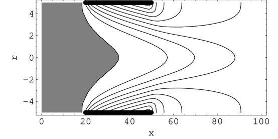
Figure 2: Concentration contours on a cross section through the vessel, including the axis ($r=0$) in the middle and the walls ($r=\pm R$) at the top and bottom. The gray area shows the region where the concentration from the target is below that of the background concentration. The thick black lines along the vessel wall mark the extent of the target region. The vertical and horizontal scales are different: the cross section is $10\mbox{$\mu$m}$ vertically and $100\mbox{$\mu$m}$ horizontally. Numbers along the axes denote distances in microns.

We suppose the source produces the chemical uniformly with flux $F_{\rm{source}}$. To evaluate high-resolution sensing capabilities, we suppose the chemical source is small, with characteristic size $L_{\rm{source}}$ as small as individual cells. Total target surface area is $2\pi RL_{\rm{source}}\approx 940\mbox{$\mu$m}^{2}$, about the same as the surface area of a single endothelial cell lining a blood vessel. The value for $F_{\rm{source}}$ in Table 1 corresponds to $5\times 10^{4}\,\mbox{molecule}/\mbox{s}$ from the source area as a whole. This flux was chosen to make the concentration at the source area equal to that given in Table 1. The background concentration is the level of the chemical when there is no injury.

Objects, such as robots, moving in the fluid alter the fluid’s velocity to some extent. For simplicity, and due to the relatively small volume of the vessel occupied by the robots, we ignore these changes and treat the fluid flow as constant in time and given by Eq. (2). Similarly, we also treat detection as due to absorbing spheres with concentration $C$ at the location of the center of the sphere for Eq. (1), assuming the robot does not significantly alter the average concentration around it. Fig. 2 shows the resulting steady-state concentration from solving Eq. (4) with $\partial C/\partial t=0$ The concentration decreases with distance from the source and the high concentration contours occur downstream of the source due to the fluid flow.

4.3 Control

parameter	value
measurement time	$T_{\rm{measure}}=10\mbox{ms}$
detection threshold	$C_{\rm{threshold}}$

Table 2: Robot control parameters for chemical signal detection.

The limited capabilities of the robots and the need to react on millisecond time scales leads to emphasizing simple controls based on local information. For chemical detection at low concentrations, the main sensor limitation is the time required for molecules to diffuse to the sensor. Thus the detections are a stochastic process. A simple decision criterion for a robot to determine whether it is near a source is if a sufficient number of detections occur in a short time interval. Specifically, a robot considers a signal detected if the robot observes at least $C_{\rm{threshold}}$ counts in a measurement time interval $T_{\rm{measure}}$. The choice of measurement time must balance having enough time to receive adequate counts, thereby reduce errors due to statistical fluctuations, while still responding before the robot has moved far downstream of the source where response would give poor localization of the source or, if robots are to take some action near the source, require moving upstream against the fluid flow. Moreover, far downstream of the source the concentration from the target is small so additional measurement time is less useful. A device passing through a vessel with a source will have about $L_{\rm{source}}/v_{\rm{avg}}=30\mbox{ms}$ with high concentration, so a measurement time of roughly this magnitude is a reasonable choice, as selected in Table 2. A low value for $C_{\rm{threshold}}$ will produce many false positives, while a high value means many robots will pass the source without detecting it (i.e., false negatives). False negatives increase the time required for detection while false positives could lead to inappropriate subsequent activities (e.g., releasing a drug to treat the injury or infection at a location where it will not be effective).

4.4 Analysis of Behavior

Task performance depends on the rate robots detect the source as they move past it, and the rate robots incorrectly conclude they detect the source due to background concentration of the chemical.

From the values of Table 1, robots enter any given vessel at an average rate

$$\omega_{\rm{robot}}=\rho_{\rm{robot}}\pi R^{2}v_{\rm{avg}}\approx 0.016/\mbox{s}$$ (5)

and the rate robots enter (and leave) any of the small vessels within the tissue volume is

$$\Omega_{\rm{robot}}=\rho_{\rm{vessel}}V\omega_{\rm{robot}}\approx 8\times 10^{3}/\mbox{s}$$ (6)

A robot encounters changing chemical concentration as it moves past the source. The expected number of counts a robot at position ${\bf r}$ has received from the source chemical during a prior measurement interval time $T_{\rm{measure}}$ is

$$K({\bf r})=4\pi Da\int_{0}^{T_{\rm{measure}}}C({\bf r}^{\prime}({\bf r},\tau))d\tau$$ (7)

where ${\bf r}^{\prime}({\bf r},\tau)$ denotes the location the robot had at time $\tau$ in the past. During the time the robot passes the target, Brownian motion displacement is $\sim 0.1\mbox{$\mu$m}$, which is small compared to the $10\mbox{$\mu$m}$ vessel diameter. Thus the possible past locations leading to ${\bf r}$ are closely clustered and for estimating the number of molecules detected while passing the target, a reasonable approximation is the robot moves deterministically with the fluid. In our axially symmetric geometry with fluid speed given by Eq. (2), positions are specified by two coordinates ${\bf r}=(r,x)$ so ${\bf r}^{\prime}((r,x),\tau)=(r,x-v(r)\tau)$ when the robot moves passively with the fluid and Brownian motion is ignored. During this motion, the robot will, on average, also encounter

$$k=4\pi DacT_{\rm{measure}}$$ (8)

molecules from the background concentration, not associated with the source.

With diffusive motion of the molecules, the actual number of counts is a Poisson distributed random process. The detection probability, i.e., having at least $E$ events when the expected number is $\mu$, is

$$\Pr(\mu,E)=1-\sum_{n=0}^{E-1}\mbox{Po}(\mu,n)$$

where $\mbox{Po}(\mu,n)=e^{-\mu}\mu^{n}/n!$ is the Poisson distribution.

Taking the devices to be ideal absorbing spheres for the chemical described in Table 1, Eq. (1) gives the capture rates $\gamma\approx 8/\mbox{s}$ at the background concentration and $\approx 2300/\mbox{s}$ near the source. Detection over a time interval $\Delta t$ is a Poisson process with mean number of detections $\mu=\gamma\Delta t$. Consider a robot at ${\bf r}$. During a small time interval $\Delta t$ the probability to detect a molecule is $4\pi Da(C({\bf r})+c)\Delta t\ll 1$. For a robot to first conclude it has detected a signal during this short time it must have $C_{\rm{threshold}}-1$ counts in the prior $T_{\rm{measure}}-\Delta t$ time interval and then one additional count during $\Delta t$. Thus the rate at which robots first conclude they detect a signal is

$$4\pi Da(C+c)\frac{\mbox{Po}(K+k,C_{\rm{threshold}}-1)}{\sum_{n<C_{\rm{threshold}}}\mbox{Po}(K+k,n)}$$ (9)

In Eq. (9) $C$ and $K$ depend on robot position and the last factor is the probability the robot has $C_{\rm{threshold}}-1$ counts in its measurement time interval, given it has not already detected the signal, i.e., the number of counts is less than $C_{\rm{threshold}}$. This expression is an approximation: ignoring correlations in the likelihood of detection over short time intervals. Eq. (9) also gives the detection rate when there is no source, i.e., false positives, by setting $C$ and $K$ to zero.

To evaluate the rate robots detect the source as they pass it, we view the robots as having two internal control states: MONITOR and DETECT. Robots are initially in the MONITOR state, and switch to the DETECT state if they detect the chemical, i.e., have at least $C_{\rm{threshold}}$ counts during time $T_{\rm{measure}}$. Using the stochastic analysis approach to evaluating robot behavior, the steady-state concentrations of robots monitoring for the chemical, $R_{\rm{m}}$, is governed by Eq. (4) for $R_{\rm{m}}$ instead of chemical concentration, with the addition of a decay due to robots changing to the DETECT state, i.e.,

$$\nabla\cdot(D_{\rm{robot}}\nabla R_{\rm{m}}-{\bf v}R_{\rm{m}})-{\alpha_{\rm{m}\rightarrow\rm{d}}}R_{\rm{m}}=0$$ (10)

The signal detection transition, ${\alpha_{\rm{m}\rightarrow\rm{d}}}$, is given by Eq. (9) and depends on the choice of threshold $C_{\rm{threshold}}$ and robot position.

The rate sensors detect the source using a threshold $C_{\rm{threshold}}$ is

$$\omega_{\rm{source}}=\omega_{\rm{robot}}\int{\alpha_{\rm{m}\rightarrow\rm{d}}}R_{\rm{m}}dV$$ (11)

where $\omega_{\rm{robot}}$ is given by Eq. (5) and the integral is over the interior volume of the vessel containing the source.

The background concentration can give false positives, i.e., occasionally producing enough counts to reach the count threshold in time $T_{\rm{measure}}$. The background concentration extends throughout the tissue volume giving many opportunities for false positives. With the parameters of Table 1, the expected count from background in $T_{\rm{measure}}$ is $\mu_{\rm{background}}=0.08$. Since a sensor spends $\approx L/v_{\rm{avg}}=1\mbox{s}$ in a small vessel in the tissue volume, the sensor has about 100 independent $10\mbox{ms}$ opportunities to accumulate counts toward the detection threshold $C_{\rm{threshold}}$. The rate of false positive detections is then

$$\omega_{\rm{background}}\approx 100\;\Omega_{\rm{robot}}\Pr(\mu_{\rm{background}},C_{\rm{threshold}})$$ (12)

For a diagnostic task, we can pick a detection threshold $C_{\rm{threshold}}$ and a time $T$ for sensors to accumulate counts. The expected number of sensors reporting detections from the source and from the background are then $\omega_{\rm{source}}T$ and $\omega_{\rm{background}}T$, respectively. The actual number is also a Poisson process, so another decision criterion for declaring a source detected is the minimum number of sensors $n$ reporting a detection. Since expected count rate near the source is significantly larger than the background rate, the contributions to the counts from the source and background are nearly independent, so the probability for detecting a source is

$$\Pr\left((\omega_{\rm{source}}+\omega_{\rm{background}})T,n\right)$$

and similarly for the false positives with counts based only on $\omega_{\rm{background}}$.

4.5 Detection Performance

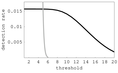
Figure 3: Rates robots detect a signal for those passing through the single small vessel with the source (black) and all the others in the tissue volume, i.e., the false positives (gray) as a function of threshold $C_{\rm{threshold}}$ used for detection during the $T_{\rm{measure}}$ time interval.

Fig. 3 shows the values of $\omega_{\rm{source}}$ and $\omega_{\rm{background}}$ for the parameters of Table 1 for various choices of the control parameter $C_{\rm{threshold}}$. Despite the much larger number of opportunities for false positives compared to the single vessel with the source, the ability of robots to pass close to the source allows selecting $C_{\rm{threshold}}\approx 10$ for which false positive detections are small while still having a significant rate of true positives.

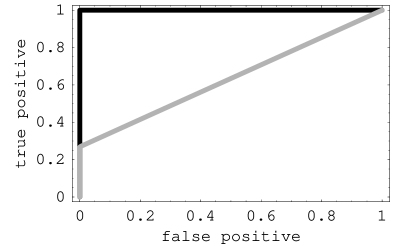
Figure 4: Probabilities of detecting a single source (true positive) and mistaking background concentration for a source (false positive) after sampling for $T=20$ and 1000 seconds (gray and solid curves, respectively). Each curve corresponds to changing the minimum threshold $C_{\rm{threshold}}$ of counts during the time interval $T_{\rm{measure}}$ required to indicate a detection event.

For diagnostics, an indication of performance is comparing the likelihood of true and false positives. In particular, identifying choices of control parameters giving both a high chance of detecting a source and a low chance of false positives. Fig. 4 illustrates the tradeoff for the task considered here. The curves range from the lower-left corner (low detection rates) with a high threshold to the upper-right corner (high detection and high false positive rate) with a low threshold. Robots collecting data for only about 20 minutes allow high performance, in this case with $C_{\rm{threshold}}$ around 10. This corresponds to the behavior seen in Fig. 3: $C_{\rm{threshold}}\approx 10$ is high enough to be rarely reached with background concentration alone (in spite of the much larger number of vessels without the source than the single vessel with the source), but still low enough that most devices passing through the single vessel with the source will detect it.

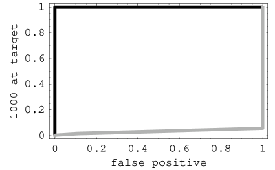
Figure 5: Probability of at least 1000 robots detecting the source vs. the probability at least one robot mistakes background concentration for a source (false positive) after sampling for $T=6\times 10^{4}$ and $10^{5}$ seconds (gray and solid curves, respectively). Each curve corresponds to changing the minimum threshold $C_{\rm{threshold}}$ of counts during the time interval $T_{\rm{measure}}$ required to indicate a detection event.

If the robots are to act at the source, ensuring at least one detection may not be enough. For instance, if the robots release a chemical near the source, or aggregate near the source (e.g., to stick to vessel wall near the source to provide enhanced imaging or to mechanically alter the tissue), then it may be necessary to ensure a relatively large number of robots detect the source. At the same time, we wish to avoid inappropriate actions due to false positives. A criterion emphasizing safety is having a high chance the required number detect the source before a single robot has a false positive detection, so not even a single inappropriate action takes place. Fig. 5 shows we can achieve high performance by this criterion: the robots circulate for about a day to have enough time for 1000 to detect the source while still having a low chance for any false positives.

Another motivation for requiring more than one detection at the source is to account for sensor failures, e.g., requiring detection by several sensors as independent confirmation of the source. Occasional spurious extra counts by the sensors amount to an increase in the effective background concentration. As long as these extra counts are infrequent, and not significantly clustered in time, such errors will not significantly affect the overall accuracy of the results.

In summary, simple control allows fast and accurate detection of even a single cell-sized source within a macroscopic tissue volume. The key feature enabling this performance is the robots’ ability to pass close to individual cells.

For comparison, instead of using microscopic sensors, one could attempt to detect the chemical from a blood sample. This allows using chemical sensors outside the body, giving simpler fabrication and use. However, such a sample dilutes the chemical throughout the blood volume, resulting in considerably smaller concentrations than are available to microscopic sensors passing close to the source. As an example, suppose a single source described above produces the chemical for one day and all this production is delivered to the blood without any degrading before a sample is taken. The source producing $\sim 5\times 10^{4}\mbox{molecule}/\mbox{s}$ gives a concentration in the 5 liter blood volume of about $7\times 10^{11}\mbox{molecule}/\mbox{m}^{3}$. This value is about $10^{-4}$ of the background concentration, so the additional chemical released by the source would be difficult to detect against small variations in background concentration.

These performance estimates also indicate behavior in other scenarios. For instance, with fewer sensors, detection times would be correspondingly longer, or would only be sensitive to a larger number of sources. For instance, with $10^{6}$ sensors, a factor of 1000 fewer than in Table 1, achieving the discrimination shown in Fig. 4 would take a thousand times longer. Alternatively, for $10^{6}$ sensors with 1000 sources distributed randomly in the tissue volume instead of just one source, performance would be similar to that shown in the figure. The stochastic analysis approach used here could also estimate other aspects of robot performance, such as the average distance to the source if and when a passing robot detects it.

Figure 6: Chemical detection probabilities vs. threshold $C_{\rm{threshold}}$ for detection during the $T_{\rm{measure}}$ time interval. Two cases are shown: a robot passing the source (black) and a robot in a small vessel without the source, i.e., false positive detection (gray). Curves are the theoretical estimates, and points are from simulations. Each point includes a line showing the 95% confidence interval of the probability estimate, which in most cases is smaller than the size of the plotted point. The points are averages from $10^{5}$ and $10^{7}$ discrete simulations of single robots passing through vessels with and without a source, respectively.

The stochastic analysis approach to evaluating robot behaviors in spatially varying fields makes various simplifying approximations to obtain $\omega_{\rm{source}}$ and $\omega_{\rm{background}}$. These include independence of the number of detection counts in different time intervals, characterizing the robots by a continuous concentration field rather than discrete objects, and ignoring how the robots (and other objects, such as blood cells) change the fluid flow and the concentration distribution of the chemical in the fluid. In principle, the analysis approach can readily include objects in the fluid, but the numerical solution becomes significantly more complicated. Instead of the parabolic velocity profile Eq. (2), fluid flow changes with time as the objects move through the vessel. Simultaneously, the object motion is determined by the drag force from the fluid. Evaluating the flow requires solving the Navier-Stokes equation, which can also include more complicated geometries for the vessels and source than treated here. Despite this additional numerical complexity, analyzing robot behaviors is formally the same.

On the other hand, history-dependent behavior of the robots, such as checking for a certain number of counts within a specified time interval, is difficult to include in the formalism, leading to the simplifying independence assumptions used here. As a check on the accuracy of these assumptions, a discrete-event simulation for the same task evaluates robot behavior without making those assumptions, but requires significantly more compute time to evaluate average behaviors. Fig. 6 shows this comparison for the key quantities used here: the detection probabilities for true and false positives. We see a fairly close correspondence between the two methods, but with a systematic error.

5 Applications for Additional Robot Capabilities

High-resolution in vivo chemical sensing with passive motion in fluids is well-suited to robots with minimal capabilities. Additional hardware capabilities allow collecting more information communicating with external observers during operation, or taking actions such as aggregating at the chemical source, releasing chemicals or mechanically manipulating the cells. This section presents a number of such possibilities.

5.1 Improved Inference from Sensor Data

The example in Fig. 4 uses a simple detection criterion based on a single choice of threshold $C_{\rm{threshold}}$. More sophisticated criteria could improve accuracy. One example is matching the temporal distribution of detections to either that expected from a uniform background or a spatially localized high concentration source. This procedure would also be useful when the source and background concentrations are not sufficiently well known a priori to determine a suitable threshold. Instead, the distribution of counts could distinguish the low background rate encountered most of the time from occasional clusters of counts at substantially higher rates.

Robots could use correlations in space or time for improved sensitivity. For instance, if a source emits several chemicals together, each of which has significant background concentration from a variety of separate sources, then detecting all of them within a short period of time improves statistical power of the inference. Similarly if the chemical is released in bursts, sensors nearby during a burst would encounter much higher local concentrations than the time averaged concentration. Stochastic temporal variation in protein production is related to the regulatory environment of the genes producing the protein, in particular the number of proteins made from each transcript [39]. Thus temporal information could identify aspects of the gene regulation within individual cells.

Correlations in the measurements could distinguish between a strong source and many weak sources throughout the tissue volume producing the chemical at the same total rate. The strong source would give high count rates for a few devices (those passing near the source) while multiple weak sources would have some detection in a larger fraction of the sensors.

As another example, using fluid flow sensors would allow correlating chemical detections with properties of the flow and the vessel geometry (e.g., branching and changes in vessel size or permeability to fluids).

5.2 Correlating Measurements from Multiple Devices

Determining properties of the chemical sources would improve if data from devices passing different sources is distinguished from multiple devices passing the same source. One possibility for correlating information from different devices is if sources, or their local environments, are sufficiently distinct chemically so measuring similar ratios of various chemicals in different devices likely indicates they encountered the same source. Common temporal variation could also suggest data from the same source.

With less distinctive sources or insufficient time to collect enough counts to make the distinction, devices capable of communicating with others nearby could provide this correlation information directly. With the parameters of Table 1, typical spacing between devices is several hundred microns, which is beyond a plausible communication distance between devices. Thus direct inter-device communication requires reducing the spacing with either a larger total number of devices or temporary local aggregation in small volumes.

Devices could achieve this aggregation if they can alter their surface properties to stick to the vessel wall [35]. With such a programmable change, a device detecting an interesting event could stick when it next encounters the wall. The parameters of Table 1 give, on average, about one device passing through a given small vessel each minute. Thus a device on the wall could remain there for a few minutes, broadcasting its unique identifier to other devices as they pass. Devices would record the identifiers they receive, with a time stamp, thereby correlating their detections.

Further inferences could be made from devices temporarily on the vessel wall where small vessels merge into larger ones. In this case, the identifier received from a device on the wall enables correlating events in nearby vessels, i.e., those that merge into the same larger vessel. Similarly, if robots aggregate in upstream vessels, before they branch into smaller ones, the robots could record each others’ unique identifiers. Subsequent measurements over the next few hundred milliseconds would be known to arise from the same region, i.e., either the same vessel or nearby ones.

The ability to selectively stick to vessel walls would allow another mode of operation: the devices could be injected in larger blood vessels leading into a macroscopic tissue volume of interest and then stick to the vessel walls after various intervals of time or when specific chemicals are detected. After collecting data, the devices would release from the wall for later retrieval.

5.3 Reporting During Operation

The devices could carry nanoscale structures with high response to external signals. Such structures could respond to light of particular wavelengths when near the skin [58], or give enhanced imaging via MRI or ultrasound [37]. Such visualization mechanisms combined with a selective ability to stick to vessel walls allows detecting aggregations of devices at specified locations near the surface of the body [52].

This visualization technique could be useful even if the tissue volume of interest is too deep to image effectively at high resolution. In particular, robots could use various areas near the skin (e.g., marked with various light or ultrasound frequencies) at centimeter scales as readout regions during operation. Devices that have detected the chemicals could aggregate at the corresponding readout location, which would then be visible externally. Devices could choose how long to remain at the aggregation points based on how high a concentration of the chemical pattern they detected. This indication of whether, and (at a coarse level) what, the devices have found could help decide how long to continue circulating to improve statistics for weak chemical signatures. These aggregation points could also be used to signal to the devices, e.g., instructing them to select among a few modes of operation.

5.4 Detection of Chemicals inside Cells

The task described above relies on detecting chemicals released into the bloodstream. However, some chemicals of interest may remain inside cells, or if released, be unable to get into the bloodstream. In that case, sensors in the bloodstream would not detect the chemical even when they pass through vessels near the cells.

However, an extension of the protocol could allow indirect detection of intracellular chemicals. For example, current technology can create molecules capable of entering cells, and, if they encounter specific chemicals, changing properties to emit signals or greatly enhance response to external imaging methods. Such molecules can indicate a variety of chemical behaviors within cells [61]. Thus if the microscopic devices include sensors for these indicator signals, they could indirectly record the activity of the corresponding intracellular chemicals in nearby cells. Such sensing from within nearby blood vessels would complement current uses of these marker molecules with much larger scale whole body imaging. In this extended protocol, the microscopic devices would provide the same benefits of detecting chemicals directly by instead detecting a proxy signal that is able to reach the nearby blood vessels.

5.5 Modifying Microenvironments

Beyond the diagnostic task discussed above, robots able to locate chemically distinctive microenvironments in the body could have capabilities to modify those environments. For instance, the devices could carry specific drugs to deliver only to cells matching a prespecified chemical profile [16, 18] as an extension of a recent in vitro demonstration of this capability using DNA computers [3].

With active locomotion, after detecting the chemicals the devices could follow the chemical gradient to the source, though this would require considerable energy to move upstream against the fluid flow. Alternatively, with sufficient number of robots so they are close enough to communicate, a robot detecting the chemical could acoustically signal upstream devices to move toward the vessel wall. In this cooperative approach, the detecting device does not itself attempt to move to the source, but rather acts to signal others upstream from the source to search for it. These upstream devices would require little or no upstream motion. Furthermore, with a large number of devices, even if only a small fraction move in the correct direction to the source after receiving a signal, many would still reach the source. This approach of using large numbers and randomness in simple local control is analogous to that proposed for collections of larger reconfigurable robots [7, 50, 51]. The behavior of microscopic active swimmers [15] raises additional control issues to exploit the hydrodynamic interactions among swimming objects as they aggregate so the distance between devices becomes only a few times their size [25].

Robots aggregated at chemically identified targets could perform precise microsurgery at the scale of individual cells. Since biological processes often involve activities at molecular, cell, tissue and organ levels, such microsurgery could complement conventional surgery at larger scales. For instance, a few millimeter-scale manipulators, built from micromachine (MEMS) technology, and a population of microscopic devices could act simultaneously at tissue and cellular size scales. An example involving microsurgery for nerve repair with plausible biophysical parameters indicates the potential for significant improvement in both speed and accuracy compared to the larger-scale machines acting alone [56, 29].

6 Discussion

Plausible capabilities for microscopic robots suggest a range of novel applications in biomedical research and medicine. Sensing and acting with micron spatial resolution and millisecond timing allows access to activities of individual cells. The large numbers of robots enable such activities simultaneously on a large population of cells in multicellular organisms. In particular, the small size of these robots allows access to tissue through blood vessels. Thus a device passes within a few tens of microns of essentially every cell in the tissue in a time ranging from tens of seconds to minutes, depending on the number of devices used.

With many devices in the tissue but only a few in the proper context to perform task, false positives are a significant issue. In some situations, these false positives may just amount to a waste of resources (e.g., power). But in other cases, too many false positives could be more serious, e.g., leading to aggregation blocking blood vessels or incorrect diagnosis.

The sensing task described in this paper highlights key control principles for microscopic robots. Specifically, by considering the overall task in a series of stages, the person using the devices remains in the decision loop, especially for the key decision of whether to proceed with manipulation (e.g., release a drug) based on diagnostic information reported by the devices. Information retrieved during treatment can also indicate whether the procedure is proceeding as planned and provide high-resolution documentation.

The performance estimates for the sensing task show devices with limited capabilities – specifically, without locomotion or communication with other devices – can nevertheless rapidly detect chemical sources as small as a single cell. The devices use their small size and large numbers to allow at least a few to get close to the source, where concentration is much higher than background. This paper also illustrates use of an analysis technique for average behavior of microscopic robots that readily incorporates spatially variable fields in the environment. Such fields are of major significance for microscopic robots, in contrast to their usual limited importance for larger robots.

As a caveat on the the results, the model examined here treats the location of the chemical source as independent of the properties and flow rates in the vessel containing the source. Systematic variation in the density and organization of the vessels will increase the variation in detected values. For instance, the tissue could have correlations between vessel density and the chemical sources (e.g., if those chemicals enhance or inhibit growth of new vessels). Accurate inference require models of how the chemicals move through the tissue to nearby blood vessels. Chemicals could react after release from the source to change the concentrations with distance from the source. Nevertheless, the simple model discussed here indicates the devices could have high discrimination for sources as small as single cells. Thus even with some unmodeled sources of variability, good performance could still be achieved by extending the sensing time or using more sophisticated inference methods. Moreover, with some localization during operation, the devices themselves could estimate some of this variation (e.g., changes in density of vessels in different tissue regions), and these estimates could improve the inference instead of relying on average or estimated values for the tissue structure.

Further open questions include the effect of higher diffusion from mixing due to motion of cells in fluid, for both chemicals and robots. For instance, the hydrodynamic effect of blood cells moving in the fluid greatly increases the diffusion coefficient of smaller objects in the fluid, to about $1000\mbox{$\mu$m}^{2}/\mbox{s}$ [33].

Instead of flowing with fluid, the sensors could be implanted at specific locations of interest to collect data in their local environments, and later retrieved. This approach does not take full advantage of the sensor size: it could be difficult to identify interesting locations at cell-size resolutions and implant the devices accurately. Nevertheless, such implants could be useful by providing local signals to indicate regions of interest to other sensors passing nearby in a moving fluid.

Safety is important for medical applications of microscopic robots. Thus, evaluating a control protocol should consider its accuracy allowing for errors, failures of individual devices or variations in environmental parameters. For the simple distributed sensing discussed in this paper, statistical aggregation of many devices’ measurements provides robustness against these variations, a technique recently illustrated using DNA computing to respond to patterns of chemicals [3]. Furthermore, the devices must be compatible with their biological environment [44] for enough time to complete their task. Appropriately engineered surface coatings and structures [17] should prevent unwanted inflammation or immune system reactions during robot operation. However, even if individual devices are inert, too many in the circulation would be harmful. From Table 1, sensors occupy a fraction $(4/3)\pi a^{3}\rho_{\rm{robot}}\approx 10^{-6}$ of the volume inside the vessels. This value is well below the fraction, about $10^{-3}$, of micron-size particles experimentally demonstrated to be safely tolerated in the circulatory system of at least some mammals [17]. Thus the number of sensors used in the protocol of this paper is unlikely to be a safety issue.

Despite the simplifications used to model sensor behavior, the estimates obtained in this paper with plausible biophysical parameters show high-resolution sensing is possible with passive device motion in the circulatory system, even without communication capabilities. Thus relatively modest hardware capabilities could provide useful in vivo sensing capabilities. Research studies of tissue microenvironments with such devices will enable better inferences from their data and indicate distributed controls suitable for more capable devices.

References

- [1] Ernesto Andrianantoandro, Subhayu Basu, David K. Karig, and Ron Weiss. Synthetic biology: New engineering rules for an emerging discipline. Molecular Systems Biology, 2(msb4100073):E1–E14, 2006.
- [2] Daniel Arbuckle and Aristides A. G. Requicha. Active self-assembly. In Proc. of the IEEE Intl. Conf. on Robotics and Automation, pages 896–901, 2004.
- [3] Yaakov Benenson, Binyamin Gil, Uri Ben-Dor, Rivka Adar, and Ehud Shapiro. An autonomous molecular computer for logical control of gene expression. Nature, 429:423–429, 2004.
- [4] Howard C. Berg. Random Walks in Biology. Princeton Univ. Press, 2nd edition, 1993.
- [5] Howard C. Berg and Edward M. Purcell. Physics of chemoreception. Biophysical Journal, 20:193–219, 1977.
- [6] Jose Berna et al. Macroscopic transport by synthetic molecular machines. Nature Materials, 4:704–710, 2005.
- [7] Hristo Bojinov, Arancha Casal, and Tad Hogg. Multiagent control of modular self-reconfigurable robots. Artificial Intelligence, 142:99–120, 2002. Available as arxiv.org preprint cs.RO/0006030.
- [8] Eric Bonabeau, Marco Dorigo, and Guy Theraulaz. Swarm Intelligence: From Natural to Artificial Systems. Oxford University Press, Oxford, 1999.
- [9] Arancha Casal, Tad Hogg, and Adriano Cavalcanti. Nanorobots as cellular assistants in inflammatory responses. In J. Shapiro, editor, Proc. of the 2003 Stanford Biomedical Computation Symposium (BCATS2003), page 62, Oct. 2003. Available at http://bcats.stanford.edu.
- [10] Adriano Cavalcanti and Robert A. Freitas Jr. Autonomous multi-robot sensor-based cooperation for nanomedicine. Intl. J. of Nonlinear Sciences and Numerical Simulation, 3:743–746, 2002.
- [11] C. P. Collier et al. Electronically configurable molecular-based logic gates. Science, 285:391–394, 1999.
- [12] H. G. Craighead. Nanoelectromechanical systems. Science, 290:1532–1535, 2000.
- [13] Amit Dhariwal, Gaurav S. Sukhatme, and Aristides A. G. Requicha. Bacterium-inspired robots for environmental monitoring. In Proc. of the IEEE Intl. Conf. on Robotics and Automation, pages 1436–1443, 2004.
- [14] K. Eric Drexler. Nanosystems: Molecular Machinery, Manufacturing, and Computation. John Wiley, NY, 1992.
- [15] Remi Dreyfus et al. Microscopic artificial swimmers. Nature, 437:862–865, 2005.
- [16] Robert A. Freitas Jr. Nanomedicine, volume I: Basic Capabilities. Landes Bioscience, Georgetown, TX, 1999. Available at www.nanomedicine.com/NMI.htm.
- [17] Robert A. Freitas Jr. Nanomedicine, volume IIA: Biocompatibility. Landes Bioscience, Georgetown, TX, 2003. Available at www.nanomedicine.com/NMIIA.htm.
- [18] Robert A. Freitas Jr. Pharmacytes: An ideal vehicle for targeted drug delivery. Journal of Nanoscience and Nanotechnology, 6:2769–2775, 2006.
- [19] J. Fritz et al. Translating biomolecular recognition into nanomechanics. Science, 288:316–318, 2000.
- [20] Y. C. Fung. Biomechanics: Circulation. Springer, NY, 2nd edition, 1997.
- [21] Aram Galstyan, Tad Hogg, and Kristina Lerman. Modeling and mathematical analysis of swarms of microscopic robots. In P. Arabshahi and A. Martinoli, editors, Proc. of the IEEE Swarm Intelligence Symposium (SIS2005), pages 201–208, 2005.
- [22] V. Gazi and K. M. Passino. Stability analysis of social foraging swarms. IEEE Trans. on Systems, Man and Cybernetics, B34:539–557, 2004.
- [23] Shankar Ghosh et al. Carbon nanotube flow sensors. Science, 299:1042–1044, 2003.
- [24] P. L. Gourley et al. Ultrafast nanolaser flow device for detecting cancer in single cells. Biomedical Microdevices, 7:331–339, 2005.
- [25] Juan P. Hernandez-Ortiz, Christopher G. Stoltz, and Michael D. Graham. Transport and collective dynamics in suspensions of confined swimming particles. Physical Review Letters, 95:204501, 2005.
- [26] Tad Hogg. Coordinating microscopic robots in viscous fluids. Autonomous Agents and Multi-Agent Systems, 2006.
- [27] Tad Hogg and Bernardo A. Huberman. Dynamics of large autonomous computational systems. In Kagan Tumer and David Wolpert, editors, Collectives and the Design of Complex Systems, pages 295–315. Springer, New York, 2004.
- [28] Tad Hogg and Philip J. Kuekes. Mobile microscopic sensors for high-resolution in vivo diagnostics. Nanomedicine: Nanotechnology, Biology, and Medicine, 2006.
- [29] Tad Hogg and David W. Sretavan. Controlling tiny multi-scale robots for nerve repair. In Proc. of the 20th Natl. Conf. on Artificial Intelligence (AAAI2005), pages 1286–1291. AAAI Press, 2005.
- [30] Joe Howard. Molecular motors: Structural adaptations to cellular functions. Nature, 389:561–567, 1997.
- [31] Charles A. Janeway et al. Immunobiology: The Immune System in Health and Disease. Garland, 5th edition, 2001.
- [32] George E. M. Karniadakis and Ali Beskok. Micro Flows: Fundamentals and Simulation. Springer, Berlin, 2002.
- [33] Kenneth H. Keller. Effect of fluid shear on mass transport in flowing blood. In Proc. of Federation of American Societies for Experimental Biology, pages 1591–1599, Sept.-Oct. 1971.
- [34] Balazs L. Keszler, Istvan J. Majoros, and James R. Baker Jr. Molecular engineering in nanotechnology: Structure and composition of multifunctional devices for medical application. In Proc. of the Ninth Foresight Conference on Molecular Nanotechnology, 2001.
- [35] Joerg Lahann and Robert Langer. Smart materials with dynamically controllable surfaces. MRS Bulletin, 30:185–188, March 2005.
- [36] Kristina Lerman et al. A macroscopic analytical model of collaboration in distributed robotic systems. Artificial Life, 7:375–393, 2001.
- [37] Jun Liu et al. Nanoparticles as image enhancing agents for ultrasonography. Physics in Medicine and Biology, 51:2179–2189, 2006.
- [38] M. Mataric. Minimizing complexity in controlling a mobile robot population. In Proc. of the 1992 IEEE Intl. Conf. on Robotics and Automation, pages 830–835, 1992.
- [39] Harley H. McAdams and Adam Arkin. Stochastic mechanisms in gene expression. Proc. Natl. Acad. Sci. USA, 94:814–819, 1997.
- [40] C. William McCurdy et al. Theory and modeling in nanoscience. workshop report, www.science.doe.gov/bes/reports/files/tmn_rpt.pdf, US Dept. of Energy, 2002.
- [41] Carlo Montemagno and George Bachand. Constructing nanomechanical devices powered by biomolecular motors. Nanotechnology, 10:225–231, 1999.
- [42] Kelly Morris. Macrodoctor, come meet the nanodoctors. The Lancet, 357:778, March 10 2001.
- [43] Frank Natterer. The Mathematics of Computerized Tomography. Soc. for Industrial and Applied Math (SIAM), Philadelphia, 2001.
- [44] Andre Nel et al. Toxic potential of materials at the nanolevel. Science, 311:622–627, 2006.
- [45] NIH. National Institutes of Health roadmap: Nanomedicine, 2003. Available at http://nihroadmap.nih.gov/nanomedicine/index.asp.
- [46] Fernando Patolsky and Charles M. Lieber. Nanowire nanosensors. Materials Today, 8:20–28, April 2005.
- [47] E. M. Purcell. Life at low Reynolds number. American Journal of Physics, 45:3–11, 1977.
- [48] Aristides A. G. Requicha. Nanorobots, NEMS and nanoassembly. Proceedings of the IEEE, 91:1922–1933, 2003.
- [49] Ingmar H. Riedel et al. A self-organized vortex array of hydrodynamically entrained sperm cells. Science, 309:300–303, 2005.
- [50] D. Rus and M. Vona. Self-reconfiguration planning with compressible unit modules. In Proc. of the Conference on Robotics and Automation (ICRA99). IEEE, 1999.
- [51] B. Salemi, W.-M. Shen, and P. Will. Hormone controlled metamorphic robots. In Proc. of the Intl. Conf. on Robotics and Automation (ICRA2001), 2001.
- [52] Robert F. Service. Nanotechnology takes aim at cancer. Science, 310:1132–1134, 2005.
- [53] Paul E. Sheehan and Lloyd J. Whitman. Detection limits for nanoscale biosensors. Nano Letters, 5(4):803–807, 2005.
- [54] Ricky K. Soong et al. Powering an inorganic nanodevice with a biomolecular motor. Science, 290:1555–1558, 2000.
- [55] Todd M. Squires and Stephen R. Quake. Microfluidics: Fluid physics at the nanoliter scale. Reviews of Modern Physics, 77:977–1026, 2005.
- [56] D. Sretavan, W. Chang, C. Keller, and M. Kliot. Microscale surgery on axons for nerve injury treatment. Neurosurgery, 57(4):635–646, 2005.
- [57] Steven Vogel. Life in Moving Fluids. Princeton Univ. Press, 2nd edition, 1994.
- [58] H. Wang et al. In vitro and in vivo two-photon luminescence imaging of single gold nanorods. Proc. of the Natl. Acad. Sci. USA, 102:15752–15756, 2005.
- [59] S.-Y. Wang and R. Stanley Williams, editors. Nanoelectronics, volume 80. Springer, March 2005. Special issue of Applied Physics A.
- [60] Zhong Lin Wang and Jinhui Song. Piezoelectric nanogenerators based on zinc oxide nanowire arrays. Science, 312:242–246, 2006.
- [61] X. Sunney Xie, Ji Yu, and Wei Yuan Yang. Living cells as test tubes. Science, 312:228–230, 2006.