Mixing and non-mixing local minima of the entropy contrast for blind source separation

Abstract

In this paper, both non-mixing and mixing local minima of the entropy are analyzed from the viewpoint of blind source separation (BSS); they correspond respectively to acceptable and spurious solutions of the BSS problem. The contribution of this work is twofold. First, a Taylor development is used to show that the exact output entropy cost function has a non-mixing minimum when this output is proportional to any of the non-Gaussian sources, and not only when the output is proportional to the lowest entropic source. Second, in order to prove that mixing entropy minima exist when the source densities are strongly multimodal, an entropy approximator is proposed. The latter has the major advantage that an error bound can be provided. Even if this approximator (and the associated bound) is used here in the BSS context, it can be applied for estimating the entropy of any random variable with multimodal density.

I Introduction

Blind source separation (BSS) aims at recovering a vector of independent sources ${\bf S}=[S_{1},\cdots,S_{K}]^{\rm T}$ from observed mixtures ${\bf X}=[X_{1},\cdots,X_{M}]^{\rm T}$. In this paper, we assume that $K=M$ and ${\bf X}={\bf A}{\bf S}$, where ${\bf A}$ is the $K$-by-$K$ mixing matrix. The sources can be recovered by finding an unmixing matrix ${\bf B}$ such that ${\bf W}={\bf B}{\bf A}$ is non-mixing (i.e. with one non-zero entry per row and per column). Such matrices ${\bf B}$ can be found by minimizing an ad-hoc cost function (see [1], the books [2, 3, 4] and references therein).

In practice, the minimum of these criteria is reached by adaptive methods such as gradient descents. Therefore, one has to pay attention to the solutions corresponding to these minima. In most of cases, the global minimum is a solution of the BSS problem. By contrast, the possible local minima can either correspond to a desired solution (referred as non-mixing minima) or spurious solution (referred as mixing minima) of the problem. For example, the optimization algorithm could be trapped in minima that do not correspond to an acceptable solution of the BSS problem. Therefore, it is of interest to study the possible existence of both non-mixing and mixing local minima.

The paper deals with this issue by extending existing results of related work. The introduction first presents the two main approaches for source separation and details the state-of-the-art related to the local minima of BSS criteria. Then, the objectives and the organization of the paper is presented.

I-A Symmetric and deflation approaches

To determine matrix ${\bf B}$, two approaches can be investigated. The first one (called symmetric) aims at extracting all sources simultaneously. The second approach (called deflation) extracts the sources one by one.

• The common symmetric approach consists in minimizing the Kullback-Leibler divergence between the joint density and the product of the marginal densities of the recovered sources (i.e. their mutual information), which are the components $Y_{1},\dots,Y_{K}$ of ${\bf Y}={\bf B}{\bf X}$. This leads to the minimization of (see [5, 6, 7])

  $$C({\bf B})=\sum_{i=1}^{K}H(Y_{k})-\log|\det{\bf B}|\enspace,$$ (1)

  where $H(Y)$ denotes Shannon’s differential entropy $Y$ [5, 6]:

  $$H(Y)=-\int p_{Y}(y)\log(p_{Y}(y))dy\enspace.$$ (2)

  In eq. (2), $p_{Y}$ denotes the probability density function (pdf) of $Y$. A variant of this approach applies the unmixing matrix ${\bf B}$ to a whitened version of the observations. In this case, since the sources are uncorrelated and can be assumed to have the same variance, one can constrain ${\bf B}$ to be orthogonal [2]. The term $\log\det{\bf B}$ in criterion (1) disappears and $C({\bf B})$ is to be minimized over the group of orthogonal matrices.

• The deflation approach [8] extracts the $k$-th source by computing the $k$-th row ${\bf b}_{k}$ of ${\bf B}$ by minimizing a non Gaussianity index of ${\bf b}_{k}{\bf X}$ subject to the constraint that ${\bf b}_{k}{\bf X}$ is uncorrelated to ${\bf b}_{i}{\bf X}$ for $i<k$. By taking this index to be the negentropy [9] and assuming (without loss of generality) that the sources have the same variance, the cost function can be written as $H({\bf w}_{k}{\bf S})-\log\|{\bf w}_{k}\|$ plus a constant, where ${\bf w}_{k}={\bf b}_{k}{\bf A}$ and $\|{\bf w}_{k}\|$ denotes the Euclidean norm $\sqrt{{\bf w}_{k}{\bf w}_{k}^{T}}$ [10, 11]. Since this function is unchanged when ${\bf w}_{k}$ is multiplied by a scalar, this leads to minimizing $H({\bf w}_{k}{\bf S})$ under the ${\bf w}_{i}{\bf w}_{k}^{\rm T}=\delta_{i,k}$ constraint for $1\leq i,k\leq K$, where $\delta_{i,k}$ is the Kronecker delta [12].

I-B Related works

Although both symmetric and deflation procedures could be analyzed in this contribution with the same tools, we focus on the entropy $H(Y_{k})$, used in the deflation approach.

Several results exist regarding the entropy minima of $Y={\bf w}{\bf S}$ (the subscript “$k$” has been omitted in the following, since one signal is extracted at a time in the deflation approach). The first kind of results discusses the existence of non-mixing local minima of $H(Y)$ that correspond to the extraction of a single source. The second kind of results discusses the existence of mixing minima that correspond to spurious solutions of the BSS problem: $Y$ is still a mixture of sources despite the fact that $H(Y)$ is a local minimum. These results are summarized below.

• Non-mixing entropy local minima
  It has been shown that the global minimum of $H(Y)$ with $Y={\bf w}{\bf S}$ is reached when the output $Y$ is proportional to the source with the lowest entropy [10]. It is proven in [9] that when a fixed-variance output is proportional to one of the sources, then, under some technical conditions, the cumulant-based approximation of entropy $H_{J}(Y)$ used in FastICA [9] reaches a non-mixing local minimum. Finally, based on the entropy power inequality [13], it is also proven in [14] that, in the two-dimensional case, Shannon’s entropy has a local minimum when the output is proportional to a non-Gaussian source.

• Mixing entropy local minima
  As for the mutual information, simulations results in [15] suggest that mixing local entropy minima exist in specific cases (i.e. when the source pdfs are strongly multimodal, which sometimes occur in practice, for sinusoid waveforms among other). These results, based on density estimation using the Parzen kernel method, are confirmed by other simulations using directly entropy estimation, such as Vasicek’s one in [16] or based on the approximator analyzed in this paper in [17]. Rigorously speaking, the above results do not constitute an absolute proof since error bounds are not available for the approximation procedure. By contrast, a theoretical proof is given in [18], but for a specific example only (two bimodal sources sharing the same symmetric pdf). The existence of mixing local entropy minima has also been shown in [19] (without detailed proof) in the case of two non symmetric sources with strongly multimodal pdfs.

I-C Objectives and organization of the paper

In this paper, additional results regarding mixing and non-mixing entropy minima are presented. Two main results will be proven.

Firstly, it will be shown in the next section that the exact entropy of an output $H(Y)$ with a fixed variance has local non-mixing minima: the entropy $H(Y)$ has a local minimum when $Y$ is proportional to one of the non-Gaussian sources. This is an extension of the results presented in [18] to the case of $K>2$ sources. If the output is proportional to the Gaussian source (if it exists), the entropy has a global maximum. Numerical simulations illustrate these results in the $K=2$ case, for the ease of illustration.

Secondly, in Section III, an entropy approximator is presented, for which an error bound can be derived. It is suitable for variables having multimodal densities with modes having a low overlap, in the sense that its error bound converges to zero when the mode overlap becomes negligible. This approximator was mentioned in [17] and error bounds have been provided in [19] without proof. In the BSS context, when the sources have such densities, the use of this approximator makes it possible to show that the marginal entropy has local mixing minima. This approach can be applied to a wider class of source densities than the score function-based method derived in [18]. The results presented in this paper further extend those in [19] as they are not restricted to the case of $K=2$ sources. Finally, we provide a detailed proof of the bound formula for the entropy approximator.

It must be stressed that the aforementioned entropy approximator can be used for other applications that require entropy estimation of multimodal densities.

II Local non-mixing minima of output entropy

In this section, we shall prove that $H({\bf w}{\bf S})$, under the $\|{\bf w}\|=1$ constraint, reaches a local minimum at ${\bf w}={\bf I}_{j}$, the $j$-th row of the $K\times K$ identity matrix, if $S_{j}$ is non-Gaussian, or a global maximum otherwise. Note that, as it is well known, the global minimum is reached at ${\bf I}_{k}$ where $k=\arg\min_{k}H(S_{k})$.

II-A Theoretic development

The starting point is an expansion of the entropy of a random variable $Y$ slightly contaminated with another variable $\delta Y$ up to second order in $\delta Y$, which has been established in [20]:

$$H(Y+\delta Y) {}\approx{} H(Y)+{\rm E}[\psi_{Y}(Y)\delta Y]+$$ (3)

$${1\over 2}\{{\rm E}[\operatorname{var}(\delta Y|Y)\psi_{Y}^{\prime}(Y)]-[{\rm E}(\delta Y|Y)]^{\prime\,2}\}\enspace.$$

In this equation, $\psi_{Y}$ is the score function of $Y$, defined as $-(\log p_{Y})^{\prime}$, $p_{Y}$ is the pdf of $Y$, ^′ denotes the derivative, and ${\rm E}(\cdot|Y)$ and $\operatorname{var}(\cdot|Y)$ denote the conditional expectation and conditional variance given $Y$, respectively.

Assume that ${\bf w}$ is close from ${\bf I}_{j}$ so that its $i$-th component $w_{i}$ is close to 0 for $i\neq j$. Under the $\|{\bf w}\|=1$ constraint, $w_{j}=\sqrt{1-\sum_{i\neq j}w_{i}^{2}}$ and since $\sqrt{1-x}=1-\frac{1}{2}x+o(x)$, one can write

$$w_{j}=1-\frac{1}{2}\sum_{i\neq j}w_{i}^{2}+o\Big{(}\sum_{i\neq j}w_{i}^{2}\Big{)}.$$

Thus, ${\bf w}{\bf S}=S_{j}+\delta S_{j}$ with

$$\delta S_{j}=\sum_{i\neq j}w_{i}S_{i}-\frac{1}{2}\Big{(}\sum_{i\neq j}w_{i}^{2}\Big{)}S_{j}+o\Big{(}\sum_{i\neq j}w_{i}^{2}\Big{)}.$$

Therefore, applying (3) and dropping higher order terms, one gets that $H({\bf w}{\bf S})$ equals

$$\halign{\hbox to\displaywidth{$\hfil\displaystyle#\hfil$}\cr 0.0pt{\hfil$\displaystyle H(S_{j})+\Big{(}\sum_{i\neq j}w_{i}\Big{)}{\rm E}[\psi_{S_{j}}(S_{j})S_{i}]-{1\over 2}\Big{(}\sum_{i\neq j}w_{i}^{2}\Big{)}{\rm E}[\psi_{S_{j}}(S_{j})S_{j}]\hfill\cr 0.0pt{\hfil$\displaystyle\hfill{}+\frac{1}{2}\Big{\{}{\rm E}\Big{[}{\rm var}\Big{(}\sum_{i\neq j}w_{i}^{2}S_{i}\Big{|}S_{j}\Big{)}\psi_{S_{j}}^{\prime}(S_{j})\Big{]}-\Big{[}\sum_{i\neq j}w_{i}{\rm E}(S_{i}|S_{j})\Big{]}^{\prime\,2}\Big{\}}\cr 0.0pt{\hfil$\displaystyle\hfill{}+o\Big{(}\sum_{i\neq j}w_{i}^{2}\Big{)}.\crcr}}}}$$

Since the sources are mutually independent, any non-linear mapping of them is uncorrelated so that ${\rm E}[\psi_{S_{j}}(S_{j})S_{i}]=0$, for $i\neq j$. Furthermore ${\rm E}(S_{i}|S_{j})={\rm E}(S_{i})=0$ for $i\neq j$, ${\rm E}[\psi_{S_{j}}(S_{j})S_{j}]=1$ (by integration by parts), and ${\rm var}(\sum_{i\neq j}w_{i}S_{i}|S_{j})={\rm var}(\sum_{i\neq j}w_{i}S_{i})=(\sum_{i\neq j}w_{i}^{2})\sigma_{S}^{2}$ where $\sigma_{S}^{2}$ denotes the common variance of the sources. Therefore

$$H({\bf w}{\bf S}) {}={} H(S_{j})+\frac{1}{2}\Big{(}\sum_{i\neq j}w_{i}^{2}\Big{)}\{\sigma_{S}^{2}{\rm E}[\psi_{S_{j}}^{\prime}(S_{j})]-1\}$$ (4)

$$\hskip 113.81102pt+o\Big{(}\sum_{i\neq j}w_{i}^{2}\Big{)}.$$

Note that again by integration by parts, ${\rm E}[\psi_{S_{j}}^{\prime}(S_{j})]$ can be rewritten as ${\rm E}[\psi_{S_{j}}^{2}(S_{j})]$, which is precisely Fisher’s information [5]. In addition, by Schwarz’s inequality [5], one has

$$|{\rm E}\{[S_{j}-{\rm E}(S_{j})]\psi_{S_{j}}(S_{j})\}|\leq\sqrt{\sigma_{S}^{2}{\rm E}[\psi_{S_{j}}^{2}(S_{j})]}\enspace,$$

with equality if and only if $\psi_{S_{j}}$ is a linear function. But since as mentioned above ${\rm E}[\psi_{S_{j}}(S_{j})]=0$ and ${\rm E}[S_{j}\psi_{S_{j}}(S_{j})]=1$, the left hand side of the above inequality equals 1. Thus $\sigma_{S}^{2}{\rm E}[\psi_{S_{j}}^{2}(S_{j})]>1$ unless $\psi_{S_{j}}$ is linear (which means that $S_{j}$ is Gaussian) in which case $\sigma_{S}^{2}{\rm E}[\psi_{S_{j}}^{2}(S_{j})]=1$. One concludes from (4) that $H({\bf w}{\bf S})>H(S_{j})$ for all ${\bf w}$ sufficiently close to ${\bf I}_{j}$ if $S_{j}$ is non-Gaussian. Thus $H({\bf w}{\bf S})$ reaches local non-mixing minima at ${\bf w}=\pm{\bf I}_{j}$ (since $H(-{\bf w}{\bf S})=H({\bf w}{\bf S})$), as long as $S_{j}$ is non-Gaussian. If $S_{j}$ is Gaussian then $H(S_{j})$ is a global maximum since Gaussian random variables have the highest entropy for a given variance. Equality (4) is of no use in this case, since the second term in this equality vanishes.

II-B Numerical simulations

In this subsection, three simple examples are analyzed in the $K=2$ case. In this case, the unit-norm vector ${\bf w}$ can be rewritten as $[\sin\theta,~{}\cos\theta]$ and $H({\bf w}{\bf S})$ is considered as a function of $\theta$. The entropy is computed through eq. (2), in which the pdf were estimated from a finite sample set (1000 samples), using Parzen density estimation [21, 22] with Gaussian Kernels of standard deviation $\sigma_{K}=0.5\hat{\sigma}_{X}*S^{-1/5}$ ($S$ denotes the number of samples and $\hat{\sigma}_{X}$ is the empirical standard deviation, enforced to be equal to one here) and Riemannian summation instead of exact integration.

Example 1

Assume that $S_{1}$ and $S_{2}$ have uniform densities. According to the above results, local minima exist for $\theta\in\{p\pi/2|p\in\mathbb{Z}\}$. In this example, no mixing minimum can be observed (Fig. 1(a)).

Example 2

Suppose now that $S_{1}$ and $S_{2}$ have uniform and Gaussian distributions respectively. Local minima are found for $\theta\in\{(2p+1)\pi/2\}$, $p\in\mathbb{Z}$, and local maxima for $\theta\in\{p\pi\}$ (Fig. 1(b)). Again, no spurious minimum can be observed in this example.

Example 3

Consider two source symmetric pdfs $p_{s_{1}}$ and $p_{s_{2}}$ that are constituted by i) two non-overlapping uniform modes and ii) two Gaussian modes with negligible overlap, respectively. One can observe that non-mixing solutions occur for $\theta\in\{p\pi/2\}$ (Fig. 1(c)).

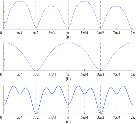
Figure 1: Evolution of of $H({\bf w}{\bf S})$ vs $\theta$: (a) Example 1: two Uniform sources (b) Example 2: Uniform ($S_{1}$) and Gaussian ($S_{2}$) sources; (c) Example 3: two bimodal sources. The non-mixing minima are indicated by dash-dotted vertical lines, the mixing ones by dotted lines.

In addition to an illustration of the above theoretical result, the last example shows the existence os spurious (mixing) local minima for $\theta\notin\{p\pi/2\}$. However, the figure does not constitute a proof of the existence of local minima of $H({\bf w}{\bf S})$; the minima visible on the figure could indeed be a consequence of the entropy estimator (more precisely, of the pdf estimation). In the next section, we derive an entropy estimator and an associated error bound. This approximator is efficient for estimating the entropy of variables having multimodal densities, in the sense that the error bound tends to zero when the mode overlaps decrease. Next, thanks to this approximator, it will be theoretically proven that mixing local minima exist for strongly multimodal source densities.

III Entropy approximator

In this section, we introduce the entropy approximator first derived in [17]. The detailed proofs of the upper and lower bounds of the entropy based on this approximator, already mentioned in [19] without proof, are given. Illustrative examples are further provided. The entropy bounds will be used in the next section to prove that for a specific class of source distributions, the entropy function $H({\bf w}{\bf S})$ can have a local minimum that does not correspond to a row of the identity matrix. The presented approach yields more general results than those in [18], since it is no longer constrained that the sources share a common symmetric pdf.

This approach relies on an entropy approximation of a multimodal pdf of the form

$$p(y)=\sum_{n=1}^{N}\pi_{n}K_{n}(y),$$ (5)

where $N>1$, $\pi_{1},\dots,\pi_{N}$ are (strictly positive) probabilities summing to 1 and $K_{1},\dots,K_{N}$ are unimodal pdfs. We focus on the case where the supports of the $K_{n}$ can be nearly covered by disjoint subsets $\Omega_{n}$ ($n=1,\dots,N$) so that $p$ is strongly multimodal (with $N$ modes). In this case a good approximation to the entropy of a random variable of density $p$ can be obtained; this entropy will be abusively denoted by $H(p)$ instead of $H(Y)$ where $Y$ is a random variable with pdf $p$. Such approximation will be first derived informally (for ease of comprehension) and then a formal development giving the error bounds of the approximator is provided.

III-A Informal derivation of entropy approximator

If the random variable has a pdf of the form (5), then its entropy equals

$$H(p)=-\int_{-\infty}^{\infty}\sum_{n=1}^{N}\pi_{n}K_{n}(y)\log\Big{[}\sum_{n=1}^{N}\pi_{n}K_{n}(y)\Big{]}dy\enspace.$$ (6)

Suppose that there exists disjoint sets $\Omega_{1},\dots,\Omega_{N}$ that nearly cover the supports of the $K_{n}$ densities; even if the $K_{n}$ have a finite support, the $\Omega_{n}$ may differ from the true support of the $K_{i}$ since these supports may be not disjoint. Then, assuming that $\pi_{n}K_{n}(y)\geq 0$ is small or zero for all $y\notin\Omega_{n}$ and noting that $0\log 0=0$ by convention (more rigorously: $\lim_{x\rightarrow 0^{+}}x\log x=0$), one gets

$$H(p) {}\approx{} -\sum_{m=1}^{N}\int_{\Omega_{m}}\sum_{n=1}^{N}\pi_{n}K_{n}(y)\log\Big{[}\sum_{n=1}^{N}\pi_{n}K_{n}(y)\Big{]}dy$$

$${}\approx{} -\sum_{m=1}^{N}\pi_{m}\int_{\Omega_{m}}K_{m}(y)\log[\pi_{m}K_{m}(y)]dy\enspace.$$

If we note $\pi=[\pi_{1},\cdots,\pi_{n}]$ and $h(\pi)\triangleq-\sum_{n=1}^{N}\pi_{n}\log\pi_{n}$ the entropy of a discrete random variable taking $N$ distinct values with probabilities $\pi_{1},\dots,\pi_{N}$, then $H(p)\approx{\cal H}(p)$ where

$${\cal H}(p)\triangleq\sum_{n=1}^{N}\pi_{n}H(K_{n})+h(\pi).$$ (7)

III-B Upper and lower bounds of the entropy of a multimodal distribution

The entropy approximator ${\cal H}(p)$ in previous subsection is actually an upper bound for the entropy. This claim is proved in the following; in addition, a lower bound of the entropy will be further provided. These bounds permit to analyze how accurate is the approximation $H(p)\approx{\cal H}(p)$; they are explicitly computed when all $K_{n}$ are Gaussian kernels.

III-B1 General results

The following Lemma provides upper and lower bounds for the entropy.

Lemma 1

Let $p$ be given by (5), then

$$H(p)\leq{\cal H}(p)$$ (8)

where ${\cal H}(p)$ is given by (7).

In addition, assume that $\sup K_{n}=\sup_{y\in\mathbb{R}}K_{n}(y)<\infty$ ($1\leq n\leq N$) and let $\Omega_{1},\dots,\Omega_{N}$ be disjoint subsets which approximately cover the supports of $K_{1},\dots,K_{N}$, in the sense that

$$\left\{\begin{array}[]{lll}\epsilon_{n}&{}\triangleq{}&\int_{\mathbb{R}\setminus\Omega_{n}}K_{n}(y)dy\enspace,\\ &&\\ \epsilon_{n}^{\prime}&{}\triangleq{}&\int_{\mathbb{R}\setminus\Omega_{n}}K_{n}(y)\log\frac{\sup K_{n}}{K_{n}(y)}dy\end{array}\right.$$ (10)

are small. Then, we have

$$H(p) {}\geq{} {\cal H}(p)-\sum_{n=1}^{N}\pi_{n}\epsilon_{n}^{\prime}$$ (11)

$$-\sum_{n=1}^{N}\pi_{n}\Big{[}\log\Big{(}\frac{\max_{1\leq m\leq N}\sup K_{m}}{\pi_{n}\sup K_{n}}\Big{)}+1\Big{]}\epsilon_{n}.$$

The proof of this Lemma is given in Appendix I.

Let us consider now the case where the densities $K_{n}$ in (5) all have the same form:

$$K_{n}(y)=(1/\sigma_{n})K[(y-\mu_{n})/\sigma_{n}]$$ (12)

where $K$ is a bounded density of finite entropy. Hence $H(K_{n})=H(K)+\log\sigma_{n}$ and the upper bound (7) becomes

$$H(p)\leq{\cal H}(p)=H(K)+\sum_{n=1}^{N}\pi_{n}\log\sigma_{n}+h(\pi).$$ (13)

Also, the lower bound of the entropy given by eq. (11) reduces to

$$H(p)\geq{\cal H}(p)-\sum_{n=1}^{N}\pi_{n}[\epsilon_{n}^{\prime}+(\log\pi_{n}^{-1}+1)\epsilon_{n}].$$ (14)

Let us arrange the $\mu_{n}$ by increasing order and take $\sigma_{n}$ small with respect to

$$d_{n}\triangleq\min(\mu_{n}-\mu_{n-1},\mu_{n+1}-\mu_{n})\enspace.$$ (15)

where $\mu_{0}=-\infty$ and $\mu_{N+1}=\infty$ by convention. Under this assumption, the density (5) is strongly multimodal and $\Omega_{n}$ in the above Lemma can be taken to be intervals centered at $\mu_{n}$ of length $d_{n}$:

$$\Omega_{n}\triangleq(\mu_{n}-d_{n}/2,\mu_{n}+d_{n}/2).$$ (16)

Then simple calculations give

$$\left\{\begin{array}[]{lll}\epsilon_{n}&{}={}&1-\int_{-d_{n}/(2\sigma_{n})}^{d_{n}/(2\sigma_{n})}K(x)dx\enspace,\\ &&\\ \epsilon_{n}^{\prime}&{}={}&H(K)-H_{d_{n}/\sigma_{n}}(K)+\epsilon_{n}\log(\sup K),\end{array}\right.$$ (19)

where $H_{\alpha}(K)\triangleq-\int_{-\alpha/2}^{\alpha/2}K(x)\log K(x)dx$. It is clear that $\epsilon_{n}$ and $\epsilon_{n}^{\prime}$ both tend to 0 as $d_{n}/\sigma_{n}\to\infty$. Thus one gets the following corollary.

Corollary 1

Let $p$ be given by (5) with $K_{n}$ of the form (12) and $\sup_{x}K(x)<\infty$. Then $H(p)$ is bounded above by ${\cal H}(p)$ and converges to this bound as $\min_{n}(d_{n}/\sigma_{n})\to\infty$, $d_{n}$ being defined in (15).

III-B2 Explicit calculation in the Gaussian case

Let us focus on the $K(x)=\Phi(x)$ case where $\Phi(x)$ denotes the standard Gaussian density: $\Phi(x)=(1/\sqrt{2\pi})\operatorname{e}^{-x^{2}/2}$.

The upper and lower bounds of $H(p)$ are given by (13) and (14) with $H(\Phi)$ instead of $H(K)$; $\epsilon_{n}$ and $\epsilon_{n}^{\prime}$ can now be obtained explicitly :

$$\left\{\begin{array}[]{lll}\epsilon_{n}=\operatorname{Erfc}\Big{(}\frac{d_{n}}{2\sqrt{2}\sigma_{n}}\Big{)},\\ &&\\ \epsilon_{n}^{\prime}=H(\Phi)-H_{d_{n}/\sigma_{n}}(\Phi)-\epsilon_{n}\log\sqrt{2\pi},\end{array}\right.$$ (21)

where $\operatorname{Erfc}$ is the complementary error function defined as $\operatorname{Erfc}(x)=(2/\sqrt{\pi})\int_{x}^{\infty}\exp(-z^{2})dz$. By double integration by parts and noting that $\int\operatorname{Erf}(x)dx=x\operatorname{Erf}(x)+\exp(-x^{2})/\sqrt{\pi}$ with $\operatorname{Erf}(x)=1-\operatorname{Erfc}(x)$, some algebraic manipulations give

$$\halign{\hbox to\displaywidth{$\hfil\displaystyle#\hfil$}\cr 0.0pt{\hfil$\displaystyle H_{d_{n}/\sigma_{n}}(\Phi)=\frac{1}{2}\operatorname{Erf}\left(\frac{d_{n}}{2\sqrt{2}\sigma_{n}}\right)\log(2\pi\operatorname{e})\hfill{}\cr 0.0pt{\hfil$\displaystyle\hfill{}-\frac{d_{n}}{2\sqrt{2\pi}\sigma_{n}}\operatorname{e}^{-d_{n}^{2}/(8\sigma_{n}^{2})}\enspace.\crcr}}}$$

One can see that $H_{d_{n}/\sigma_{n}}(\Phi)\to H(\Phi)=\log\sqrt{2\pi\operatorname{e}}$ as $d_{n}/\sigma_{n}\rightarrow\infty$, as it should be. Finally:

$$\left\{\begin{array}[]{lll}\epsilon_{n}&{}={}&\displaystyle\operatorname{Erfc}\Big{(}\frac{d_{n}}{2\sqrt{2}\sigma_{n}}\Big{)}\\ &&\\ \epsilon_{n}^{\prime}&{}={}&\displaystyle\frac{1}{2}\operatorname{Erfc}\Big{(}\frac{d_{n}}{2\sqrt{2}\sigma_{n}}\Big{)}+\frac{d_{n}}{2\sqrt{2\pi}\sigma_{n}}\operatorname{e}^{-[d_{n}/(2\sqrt{2}\sigma_{n})]^{2}}\end{array}\right..\qquad$$ (24)

Example 4

To illustrate Corollary 1, Fig. 2 plots the entropy of a trimodal variable $Y$ with density $p$ as in (5) with $K_{n}$ given by (12), $\sigma_{n}=\sigma$ (for the ease of illustration), $K=\Phi$, $\mu=[0,5,10]$ and $\pi=[1/4,1/2,1/4]$. Such variable can be represented as $Y=U+\sigma Z$ where $U$ is a discrete random variable taking values in $\{0,5,10\}$ with probabilities $1/4,1/2,1/4$ and $Z$ is a standard Gaussian variable independent from $U$. The upper and lower bounds of the entropy are computed as in Lemma 1 with the above expressions for $\epsilon_{n},~{}\epsilon_{n}^{\prime}$, and plotted on the same figure. One can see that the lower the $\sigma$, the better the approximation of $H(Y)$ by its upper and lower bounds. On the contrary, when $\sigma$ increases, the difference between the entropy and its bounds tend to increase, which seems natural. These differences however can be seen to tend towards a constant for $\sigma\to\infty$. This can be explained as follows. When $\sigma$ is large, $p$ is no longer multimodal and tends to the Gaussian density of variance $\sigma^{2}$. Thus $H(Y)$ grows with $\sigma$ as $\log\sigma$. On the other hand, the upper bound of ${\cal H}(p)$ of $H(Y)$ also grows as $\log\sigma$. The same is true for the lower bound of $H(Y)$ which equals ${\cal H}(p)-\sum_{n=1}^{3}\pi_{n}[\epsilon^{\prime}_{n}+\epsilon_{n}(\log\pi_{n}^{-1}+1)]$: the last term tends to $h(\pi)+\frac{3}{2}$ as $\sigma\to\infty$ since for fixed $d_{n}$, $\epsilon_{n}\rightarrow 1$ and $\epsilon_{n}^{\prime}\rightarrow 1/2$ as $\sigma\rightarrow\infty$.

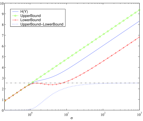
Figure 2: Illustration of Example 4: Evolution of $H(Y)$ and its bounds versus $\sigma$, where $Y=U+\sigma Z$, $U$ is a discrete random variable taking values in $\{0,5,10\}$ with probabilities $\pi=[1/4,1/2,1/4]$ and $Z$ is a standard Gaussian variable independent from $U$. The lower bound converges to the upper bound as $\sigma\rightarrow 0$ and the difference between upper and lower bounds tends to $3/2+h(\pi)$ as $\sigma\rightarrow\infty$ (note that the horizontal axis scale is logarithmic).

III-C Entropy bounds and decision theory

The entropy estimator given in eq. (7) has actually close connections with decision problems, and a tighter upper bound for $H(p)$ can be found in this framework. Assume we have a $N$-class classification problem consisting in finding the class label $C$ of an observation $y_{n}$, knowing the densities and the priors of the classes. In such kinds of classification problems, one is often interested in quantifying the Bayes’ probability of error $P(e)$. In our context, each of the pdf mode $K_{n}$ represents the density of a given class $c_{n}$, i.e. the conditional density of $Y$ given $C=c_{n}$ is $K_{n}$. Furthermore, $\pi_{n}$ is the a priori probability of $c_{n}$ : $P(C=c_{n})=\pi_{n}$, and $p$ is the density of $Y$, which can thus be seen as a “mixture density”. Defining $h(C)=-\sum_{n=1}^{N}P(C=c_{n})\log P(C=c_{n})$, it can be shown [23],[24] that

$$P(e) \leq \frac{1}{2}h(C|Y)=\frac{1}{2}[H(Y|C)+h(C)-H(Y)]$$ (25)

$$= \frac{1}{2}\bigg{[}\sum_{n=1}^{N}\pi_{n}H(K_{n})+h(\pi)-H(Y)\bigg{]}$$

where $H(Y|C)\triangleq{\rm E}_{C}[H(Y|C=c_{i})]$, which shows that half the difference between the ${\cal H}(p)$ and $H(p)$ is precisely an upper bound of Bayes’ probability of error $P(e)\triangleq{\rm E}_{Y}[1-\max_{i}p(c_{i}|y)]$. The error vanishes when the modes have no overlap (the classes are separable, i.e. disjoint).

Clearly, ${\cal H}(p)-2P(e)$ is a tighter upper bound of $H(p)$ than ${\cal H}(p)$ as $P(e)\geq 0$. On the other hand, it can be proved that ${\cal H}(p)-2\sqrt{(N-1)P(e)}$ is a lower bound for $H(p)$ [24]. However, the lower bound in Lemma 1 is tighter when $\sigma$ is small enough. Both bounds in this lemma are easier to deal with in more general theoretical developments, are more related to the multimodality of $p(y)$ and suffice for our purposes. Therefore, in the following theoretical developments, the last pair of bounds shall be used.

IV Mixing local minima in multimodal BSS

Based on the results derived in Section III-B, it will be shown that mixing local minima of the entropy exist in the context of the blind separation of multimodal sources with Gaussian modes if the mode standard deviations $\sigma_{n}$ are small enough.

We are interested in the (mixing) local minima of $H({\bf w}{\bf S})$ on the unit sphere ${\cal S}=\{{\bf w}:\|{\bf w}\|=1\}$ of $\mathbb{R}^{K}$. We shall assume that the sources have a pdf of the form (5), with $K_{n}$ being Gaussian with identical variance $\sigma^{2}$ (but with distinct means). Thus, as in example 4, we may represent $S_{k}$ as $U_{k}+\sigma Z_{k}$ where $U_{k}$ is a discrete random variable and $Z_{k}$ is a standard Gaussian variable independent from $U_{k}$. Further, $(U_{1},Z_{1}),\dots,(U_{K},Z_{K})$ are assumed to be independent so that the sources are independent as required. From this representation, ${\bf w}{\bf S}={\bf w}{\bf U}+\sigma Z$ where ${\bf U}$ is the column vector with components $U_{k}$ and $Z$ is again a standard Gaussian variable (since any linear combination of independent Gaussian variables is a Gaussian variable and $\sum_{k=1}^{K}w_{k}Z_{k}$ has zero mean and unit variance). Since ${\bf w}{\bf U}$ is clearly a discrete random variable, ${\bf w}{\bf S}$ also has a multimodal distribution of the form (5) with $K_{n}$ again the Gaussian density with variance $\sigma^{2}$. Note that the number of modes is the number of distinct values ${\bf w}{\bf U}$ can have and the mode centers (the means of the $K_{n}$) are these values; they depend of ${\bf w}$. However, as long as $\sigma$ is small enough with respect to the distances $d_{n}$ defined in (15) the approximation (7) of the entropy is justified. Thus, we are led to the approximation $H({\bf w}{\bf S})\approx h({\bf w}{\bf U})+\log\sigma+H(\Phi)$, where $h({\bf w}{\bf U})$ denotes abusively the entropy of the discrete random variable ${\bf w}{\bf U}$ (the entropy of a discrete random variable $U$ with probability vector $\pi$ is noted either $h(U)$ or $h(\pi)$).

The above approximation suggests that there is a relationship between the local minimum points of $H({\bf w}{\bf S})$ and those of $h({\bf w}{\bf U})$. Therefore, we shall first focus on the local minimum points of the entropy of ${\bf w}{\bf U}$ before analyzing those of $H({\bf w}{\bf S})$.

IV-A Local minimum points of $h({\bf w}{\bf U})$

The function $h({\bf w}{\bf U})$ does not depend on the values that ${\bf w}{\bf U}$ can take but only on the associated probabilities; these probabilities remain constant as ${\bf w}$ changes unless the number of distinct values that ${\bf w}{\bf U}$ can take varies. Such number would decrease when an equality ${\bf w}{\bf u}={\bf w}{\bf u}^{\prime}$ is attained for some distinct column vectors ${\bf u}$ and ${\bf u}^{\prime}$ in the set of possible values of ${\bf U}$. A deeper analysis yields the following result, which is helpful to find the local minimum point of $h({\bf w}{\bf U})$.

Lemma 2

Let ${\bf U}$ be a discrete random vector in $\mathbb{R}^{K}$ and $\cal U$ be the set of distinct values it can take. Assume that there exists $r\geq 1$ disjoint subsets ${\cal U}_{1},\dots,{\cal U}_{r}$ of $\cal U$ each containing at least 2 elements, such that the linear subspace $V$ spanned by the vectors ${\bf u}-{\bf u}_{1},{\bf u}\in{\cal U}_{1}\setminus\{{\bf u}_{1}\},\dots,{\bf u}-{\bf u}_{r},{\bf u}\in{\cal U}_{r}\setminus\{{\bf u}_{r}\}$, ${\bf u}_{1},\dots,{\bf u}_{r}$ being arbitrary elements of ${\cal U}_{1},\dots,{\cal U}_{r}$, is of dimension $K-1$. (Note that $V$ does not depend on the choice of ${\bf u}_{1},\dots,{\bf u}_{r}$, since ${\bf u}-{\bf u}_{j}^{\prime}=({\bf u}-{\bf u}_{j})-({\bf u}_{j}^{\prime}-{\bf u}_{j})$ for any other ${\bf u}_{j}^{\prime}\in{\cal U}_{j}$.) Then for ${\bf w}^{*}\in\cal S$ and orthogonal to $V$, there exists a neighborhood $\cal W$ of ${\bf w}^{*}$ in $\cal S$ and $\alpha>0$ such that $h({\bf w}{\bf U})\geq h({\bf w}^{*}{\bf U})+\alpha$ for all ${\bf w}\in{\cal W}\setminus\{{\bf w}^{*}\}$. In the case $K=2$, one has a stronger result that $h({\bf w}{\bf U})=h({\bf U})>h({\bf w}^{*}{\bf U})$ for all ${\bf w}\in{\cal W}\setminus\{{\bf w}^{*}\}$.

The proof is given in Appendix II.

Example 5

An illustration of Lemma 2 in the $K=2$ case (again for clarity) is provided in Fig.3. We note ${\bf U}=[U_{1},U_{2}]^{\rm T}$ where the discrete variables $U_{1}$ and $U_{2}$ take the values $-\sqrt{1.03}+2.5,\sqrt{1.03}+2.5$ with probabilities and $.5,.5$ and the values $-1.2,-.4,2$ with probabilities $1/2,3/8,1/8$, respectively. They are chosen to have the same variance, as we need that the $S_{k}=U_{k}+\sigma Z_{k}$, $k=1,2$, have the same variance. But their mean can be arbitrary since $H({\bf w}{\bf S})$ does not depend on them. In this $K=2$ example, each line that links two distinct points ${\bf u},{\bf u}^{\prime}\in{\cal U}$ span a one dimensional linear subspace, which constitutes a possible subspace $V$, as stated in Lemma 2. There are thus many possibilities for $V$, each corresponding to a specific vector ${\bf w}^{*}$.

Two simple possibilities for $V$ are the subspaces with direction given by $[0,1]^{\rm T}$ and $[1,0]^{\rm T}$. In the first case, the subsets ${\cal U}_{i}$ are built by grouping the points of ${\cal U}$ laying on a same vertical dashed line. There are two such subsets ($r=2$) consisting of ${\bf u}\in\cal U$ with first component equal to $-\sqrt{1.03}+2.5$ and $\sqrt{1.03}+2.5$, respectively. In the second case, the subsets ${\cal U}_{i}$ are built by grouping the points of ${\cal U}$ laying on a same horizontal dashed line. There are three such subsets ($r=3$) consisting of ${\bf u}\in\cal U$ with second component equal to $-1.2$, $-.4$ and 2, respectively.

There also exist other subspaces $V$, corresponding to “diagonal lines” (i.e. to solid lines in Fig.3). This last kind of one-dimensional linear subspace $V$ correspond to directions given by two-dimensional vectors ${\bf w}^{*}$ with two non-zero elements.

On the plot, the points on the half circle correspond to the vectors ${\bf w}^{*}$ of the Lemma; each ${\bf w}^{*}$ is orthogonal to a line joining a pair of distinct points in $\cal U$, $\cal U$ being the set of all possible values of $[U_{1},U_{2}]^{\rm T}$. The points of $\cal U$ are displayed in the plot together with their probabilities. The entropies $h({\bf w}{\bf U})$ are also given in the plot; one can see that they are lower for ${\bf w}={\bf w}^{*}$ than for other points ${\bf w}$.

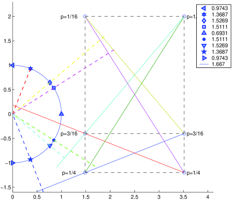
Figure 3: Example 5: illustration of Lemma 2. The discrete random variables $U_{1}$ and $U_{2}$ take values in $\{-\sqrt{1.03}+2.5,\sqrt{1.03}+2.5\}$ and $\{-1.2,-.4,2\}$ with probabilities $[.5.5]$ and $[1/2,3/8,1/8]$, respectively.

The above Lemma only provides a mean to find a local minimum point of the function $h({\bf w}{\bf U})$, but does not prove the existence of such a point, since the existence of $V$ was only assumed in the Lemma. Nevertheless, in the case where the components of ${\bf U}$ are independent and can take at least 2 distinct values, subset ${\cal U}_{i}$ ensuring the existence of $V$ can be built as follows. Let $j$ be any index in $\{1,\dots,K\}$ and $\lambda_{j,1},\dots,\lambda_{j,r_{j}}$ be the possible value of $U_{j}$, the $j$-th component of ${\bf U}$. One can take ${\cal U}_{i},1\leq i\leq r_{j}$ to be the set of ${\bf u}\in\cal U$ such that its $j$-th components equal $\lambda_{j,i}$. Then it is clear that the corresponding subspace $V$ consists of all vectors orthogonal to the $j$-th row of the identity matrix (hence $V$ is of dimension $K-1$) and that the associated vector ${\bf w}^{*}$ is simply this row or it opposite. By Lemma 2, this point ${\bf w}^{*}$ would be a local minimum point of $h({\bf w}{\bf U})$. But, as explained above, it is a non mixing point while we are interested in the mixing point, i.e. not proportional to a row of the identity matrix. However, the above construction can be extended by looking for a set of $K$ vectors ${\bf u}_{1},\dots,{\bf u}_{K}$ in $\cal U$, such that the vectors ${\bf u}_{i}-{\bf u}_{j},1\leq i<j\leq K$ span any linear subspace of dimension $K-1$ of $\mathbb{R}^{K}$. If such a set can be found, then $V$ is simply this linear subspace by taking ${\cal U}_{1}=\{{\bf u}_{1},\dots,{\bf u}_{K}\}$ and $r=1$. In addition, if ${\bf u}_{1},\dots,{\bf u}_{K}$ do not all have the same $j$-th component, for some $j$, then the corresponding ${\bf w}^{*}$ is a mixing local minimum point. In view of the fact that there are at least $2^{K}$ points in $\cal U$ to choose from for the ${\bf u}_{i}$ and that the last construction procedure meant not find all local minimum points of $h({\bf w}{\bf U})$, chance is that there exists both non-mixing and mixing local minimum points of $h({\bf w}{\bf U})$. In the $K=2$ case this is really the case: it suffices to take two distinct points ${\bf u}_{1}$ and ${\bf u}_{2}$ in $\cal U$, then by the above Lemma, the vector ${\bf w}^{*}$ orthogonal to ${\bf u}_{1}-{\bf u}_{2}$ is a local minimum point of $h({\bf w}{\bf U})$. If one choose ${\bf u}_{1}$ and ${\bf u}_{2}$ such that both components of ${\bf u}_{1}-{\bf u}_{2}$ are non zero, the associated orthogonal vector ${\bf w}^{*}$ is not proportional to any row of the identity matrix; it is a mixing local minimum point of $h({\bf w}{\bf U})$. Note that in the particular $K=2$ case, the aforementioned method identifies all local minimum points of $h({\bf w}{\bf U})$. Indeed, for any ${\bf w}\in\cal S$, either there exists a pair of distinct vectors ${\bf u}_{1},{\bf u}_{2}$ in $\cal U$ such that ${\bf w}({\bf u}_{1}-{\bf u}_{2})=0$ or there exists no such pair. In the first case ${\bf w}$ is a local minimum point and in the second case one has $h({\bf w}{\bf U})=h({\bf U})$. Since there is only a finite number of the differences ${\bf u}_{1}-{\bf u}_{2}$, for distinct ${\bf u}_{1},{\bf u}_{2}$ in $\cal U$, there can be only a finite number of local minimum points of $h({\bf w}{\bf U})$, and for all other points $h({\bf w}{\bf U})$ take the maximum value $h({\bf U})$.

IV-B Local minimum points of $H({\bf w}{\bf S})$

This subsection shows that the local minima points of $H({\bf w}{\bf S})$ can be related to those of $h({\bf w}{\bf U})$.

Lemma 3

Define $S_{i}$, $i=1,\cdots,K$, as $S_{i}=U_{i}+\sigma Z_{i}$ described at the beginning of subsection IV and ${\bf w}^{*}$ be a vector satisfying the assumption of Lemma 2 (${\bf U}$ being the vector with component $U_{i}$). Then for $\sigma$ sufficiently small $H({\bf w}{\bf S})$ admits a local minimum point converging to ${\bf w}^{*}$ as $\sigma\to 0$.

The proof of this Lemma is relegated to the Appendix.

Example 6

Thanks to the entropy approximator, we shall illustrate the existence of the local minima of $H({\bf w}{\bf S})$ in the following $K=2$ example, so that vectors ${\bf w}$ satisfying $||{\bf w}||=1$ can be written as $[\sin\theta,\cos\theta]$. We take $S_{1}=U_{\pi/2}+\sigma Z_{1}$ and $S_{2}=U_{0}+\sigma Z_{2}$, where $U_{0},U_{\pi/2}$ are independent discrete random variables taking the values $-2\sqrt{3}/3,\sqrt{3}/2$ with probabilities $1/3,2/3$ and $-\sqrt{2},\sqrt{2}/2$ with probabilities $3/7,4/7$, respectively, and $Z_{1}$, $Z_{2}$ are standard Gaussian variables. The parameter $\sigma$ is set to 0.1. Thus $Y_{\theta}={\bf w}{\bf S}$ can be represented as $U_{\theta}+\sigma Z$ where $U_{\theta}=\sin\theta U_{\pi/2}+\cos\theta U_{0}$ and $Z$ is a standard Gaussian variable independent from $U_{\theta}$. Figure 4 plots the pdf of $Y_{\theta}$ for various angles $\theta$. It can be seen that the modality (i.e. the number of modes) changes with $\theta$. Fig. 5 shows the entropy of $Y_{\theta}$ together with its upper and lower bounds, for $\theta\in[0,\pi]$. In addition to non-mixing local minima at $\theta\in\{p\pi/2|p\in\mathbb{Z}\}$, mixing local minima exist when ${\bf w}({\bf u}_{1}-{\bf u}_{2})=0$, where ${\bf u}_{1}=[-2\sqrt{3}/3,\sqrt{2}/2]^{\rm T},{\bf u}_{2}=[\sqrt{3}/2,-\sqrt{2}]^{\rm T}$, i.e. when $|\tan(\theta)|=.9526$, or $\theta\in\{(0.2423+p)\pi,(0.7577+p)\pi|p\in\mathbb{Z}\}$. One can observe that the upper bound is a constant function except for a finite number of angles for which we observe negative peaks (see Lemma 2). For these angles the pdf is strongly multimodal, and the upper and lower bounds are very close, though not clearly visible on the figure. This results from a discontinuity of the lower bound at these angles, due to the superimposition of several modes at these angles.

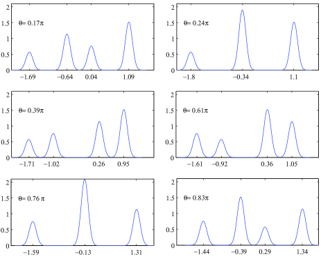
Figure 4: Example 6: probability density function of ${\bf w}{\bf S}$ for various angles $\theta$.

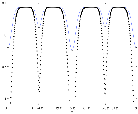
Figure 5: Example 6: Upperbound (dashed line), lower bound (dots) and entropy estimation of $Y_{\theta}$ using finite Riemannian sum (solid). It can be seen that the upper and lower bounds of the entropy converge to each other when the density becomes strongly multimodal (see the corresponding plots in Fig. 4).

V Complementary observations

This section provides two observations that can be drawn regarding the impact of the mode variance $\sigma^{2}$ on the existence of local minima and the symmetry of the entropy with respect to $\theta$.

V-A Impact of “mode variance” $\sigma^{2}$

In the example of Fig. 6 the discrete variables $U_{1}$ and $U_{2}$ in the expression of $S_{1}$ and $S_{2}$ are taken as in Example 5. One can observe that the mixing minima of the entropy tends to disappear when the mode variance increases. This is a direct consequence of the fact that the mode overlaps increase. When $\sigma$ increases, the source densities become more and more Gaussian and the $H({\bf w}{\bf S})$ vs $\theta$ curve tends to be more and more flat, approaching the constant function $\log\sqrt{2\pi\operatorname{e}}+\log\sigma$. The upper and lower bounds have only been plotted for the $\sigma=.05$, for visibility purposes. Again, at angles corresponding to the upper bound negative peaks, the error bound is very tight, as explained in Example 6.

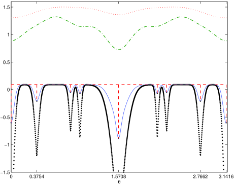
Figure 6: Entropy of ${\bf w}{\bf S}$ (estimated using finite Riemannian sum) versus $\theta$ for $S_{1}=U_{1}+\sigma Z_{1}$, $S_{2}=U_{2}+\sigma Z_{2}$, where $U_{1}$ and $U_{2}$ are taken from example 5 (and Fig. 3) and the four random variables are all independent. The parameter $\sigma$ is set to $.05$ (solid), $.25$ (dashed-dotted) and $.5$ (dotted). The upper and lower bounds have been added for the $\sigma=.05$ case only, for visibility purposes. It can be seen that the upper and lower bounds of the entropy converge to each other when the density becomes strongly multimodal.

V-B Note on symmetry of $H({\bf w}_{\theta}{\bf S})$

In the above graphs plotting the entropy (and its bounds) versus $\theta$, some symmetry can be observed. First, if we note ${\bf w}_{\theta}=[\sin\theta\cos\theta]$, observe that $H({\bf w}_{\theta}{\bf S})=H({\bf w}_{\theta+\pi}{\bf S})$ whatever are the source pdfs; this is a direct consequence of the fact the the entropy is not sign sensitive. Second, if one of the source densities is symmetric, i.e. if it exists $\mu\in\mathbb{R}$ so that $p_{S_{j}}(\mu-s)=p_{S_{j}}(\mu+s)$ for all $s\in\mathbb{R}$, then $H({\bf w}_{\theta}{\bf S})=H({\bf w}_{-\theta}{\bf S})$. Third, if the two sources share the same pdf, then $H({\bf w}_{\theta}{\bf S})=H({\bf w}_{\pi/2-\theta}{\bf S})$. Finally, if the two sources can be expressed as in Lemma 3, then the vectors ${\bf w}^{*}$ for which $h({\bf w}^{*}{\bf U})<h({\bf U})$ (as obtained in Lemma 2) are symmetric in the sense that their angles are pairwise opposite. This means that for $\sigma$ small enough, if a local minimum of $H({\bf w}_{\theta}{\bf S})$ appears at $\theta^{*}$, then another local minimum point will exist near $-\theta^{*}$ (and thus near $p\pi-\theta,\ \forall p\in\mathbb{Z})$. The above symmetry property can be seen from Figure 3 and can be proved formally as follows. From Lemma 2, ${\bf w}^{*}$ must be orthogonal to ${\bf u}_{1}-{\bf u}_{2}$ for some pair of distinct vectors in the set of all possible values of ${\bf U}$. Define ${\bf u}_{i}^{\dagger}$ ($i=1,2$) to be the vector with first coordinate the same as that of ${\bf u}_{3-i}$ and second coordinate the same as that of ${\bf u}_{i}$. Then it can be seen that the vector orthogonal to ${\bf u}_{1}^{\dagger}-{\bf u}_{2}^{\dagger}$ has an angle opposite to the angle of ${\bf w}^{*}$, yielding the desired result.

VI Conclusion

In this paper, new results regarding both non-mixing and mixing entropy local minima have been derived in the context of the blind separation of $K$ sources. First, it is shown that a local entropy minimum exists when the output is proportional to one of the non-Gaussian source. Second, it is shown that mixing entropy minima may exist when the source densities are strongly multimodal (i.e. multimodal with sufficiently small overlap); therefore, spurious BSS solutions can be obtained when minimizing this entropic criterion. Some attention must be paid to the obtained solutions when they are found by adaptive gradient minimization.

To prove the existence of mixing entropy minima, a theoretical framework using an entropy approximator and its associated error bounds has been provided. Even if this approximator is considered here in the context of blind source separation, its use can be extended to other applications involving entropy estimation.

Appendix A Proofs of Lemmas

Proof of Lemma 1 We have from (6) that $H(Y)=\sum_{n=1}^{N}\pi_{n}H_{n}$ where

$$H_{n}\triangleq-\int K_{n}(y)\log\Big{[}\sum_{m=1}^{N}\pi_{m}K_{m}(y)\Big{]}dy.$$ (26)

Since all $K_{m}\geq 0$, the last right hand side is bounded above by $-\int K_{n}(y)\log[\pi_{n}K_{n}(y)]\,dy=H(K_{n})-\log\pi_{n}$, yielding the inequality (8).

A more elegant derivation of this inequality can be obtained from the entropy properties. Indeed, the density given in (5) can be interpreted as the marginal density of an augmented model $(Y,U)$ where $U$ is a discrete variable with $N$ values $u_{1},\dots,u_{n}$ with probabilities $\pi_{1},\dots,\pi_{n}$ and $Y$ has a conditional density given $U=u_{n}$ equal to $K_{n}$. The joint entropy $H(Y,U)$ of (the “continuous-discrete” pair of random variables) $Y,U$ equals $H(Y|U)+h(U)$ where $h(U)=h(\pi)$ is the discrete entropy of $U$ and $H(Y|U)=\sum_{n=1}^{N}\pi_{n}H(K_{n})$ is the conditional entropy of $Y$ given $U$. But $H(Y,U)=h(U|Y)+H(Y)$ (where $h(U|Y)$ is the conditional entropy of $U$ given $Y$) and thus ${\cal H}(p)-H(p)$ equals $h(U|Y)$ which is always nonnegative because $U$ is a discrete variable.

Yet another way to prove the above inequality is to exploit its connection to the decision problem discussed in Section III-C. Indeed, equation (25) yields immediately ${\cal H}(p)-H(p)\geq P(e)\geq 0$.

To prove the second result, noting that $\log(1+x)\leq x$, the term $\log[\sum_{m=1}^{N}\pi_{m}K_{m}(y)]$ can be bounded above by

$$\left\{\begin{array}[]{ll}\displaystyle\log[\pi_{n}K_{n}(y)]+\sum_{1\leq m\leq N,m\neq n}\frac{\pi_{m}K_{m}(y)}{\pi_{n}K_{n}(y)}&\hbox{ if }y\in\Omega_{n}\\ \log(\max_{1\leq m\leq N}\sup K_{m})&\hbox{otherwise}\enspace.\end{array}\right.$$ (29)

Therefore, with

$$H_{n}\triangleq-\int K_{n}(y)\log\Big{[}\sum_{m=1}^{N}\pi_{m}K_{m}(y)\Big{]}dy.$$ (30)

one gets

$$H_{n} {}\geq{} -\int_{\Omega_{n}}K_{n}(y)\log[\pi_{n}K_{n}(y)]dy$$

$$-\sum_{1\leq m\leq N,m\neq n}\frac{\pi_{m}}{\pi_{n}}\int_{\Omega_{n}}K_{m}(y)dy$$

$$-\log(\max_{1\leq m\leq N}\sup K_{m})\epsilon_{n}$$

But since $\Omega_{1},\dots,\Omega_{N}$ are disjoint,

$$\halign{\hbox to\displaywidth{$\hfil\displaystyle#\hfil$}\cr 0.0pt{\hfil$\displaystyle\sum_{n=1}^{N}\pi_{n}\sum_{1\leq m\leq N,m\neq n}\frac{\pi_{m}}{\pi_{n}}\int_{\Omega_{n}}K_{m}(y)dy={}\hfill\cr 0.0pt{\hfil$\displaystyle\hfill\sum_{m=1}^{N}\pi_{m}\int_{\cup_{1\leq n\neq m\leq N}\Omega_{n}}K_{m}(y)dy,\crcr}}}$$

and $\cup_{1\leq n\neq m\leq N}\Omega_{n}\subseteq\mathbb{R}\setminus\Omega_{m}$. Therefore the right hand side of the above equality is bounded above by $\sum_{m=1}^{N}\pi_{m}\epsilon_{m}$. It follows that $H(p)=\sum_{n=1}^{N}\pi_{n}H_{n}$ is bounded below by

$$\halign{\hbox to\displaywidth{$\hfil\displaystyle#\hfil$}\cr 0.0pt{\hfil$\displaystyle h(\pi)+\sum_{n=1}^{N}\pi_{n}H(K_{n})+\sum_{n=1}^{N}\pi_{n}\log(\pi_{n}\sup K_{n})\epsilon_{n}-\sum_{n=1}^{N}\pi_{n}\epsilon_{n}^{\prime}\hfill\cr 0.0pt{\hfil$\displaystyle\hfill-\sum_{m=1}^{N}\pi_{m}\epsilon_{m}-\sum_{n=1}^{N}\pi_{n}\log(\max_{1\leq m\leq N}\sup K_{m})\epsilon_{n}\crcr}}}$$

After some manipulations, the above expression reduces to the lower bound for $\sum_{n=1}^{N}\pi_{n}H_{n}$ given in the Lemma   

Proof of Lemma 2

By construction, for each $j=1,\dots,r$, ${\bf w}^{*}{\bf u}$ take the same values for ${\bf u}\in{\cal U}_{j}$. On the other hand, by grouping the vectors ${\bf u}\in\cal U$ which produce the same value of ${\bf w}^{*}{\bf u}$ into subsets of $\cal U$, one gets a partition of $\cal U$ into $r^{*}+1$ subsets ${\cal U}_{0}^{*},\dots,{\cal U}_{r^{*}}^{*}$, such that each ${\cal U}_{j}^{*},1\leq j\leq r^{*}$ contains at least two elements and ${\bf w}^{*}{\bf u}$ takes the same values for ${\bf u}\in{\cal U}_{j}^{*}$ and the values associated with different ${\cal U}_{j}^{*}$ and the ${\bf w}^{*}{\bf u},{\bf u}\in{\cal U}_{0}^{*}$, are all distinct. Obviously $r^{*}\geq 1$ and each of the ${\cal U}_{1},\dots,{\cal U}_{r}$, must be contained in one of the ${\cal U}_{1}^{*},\dots,{\cal U}_{r^{*}}^{*}$. Therefore the space $V$ must be contained in the space spanned by the vectors ${\bf u}-{\bf u}_{j},{\bf u}\in{\cal U}_{j}^{*}\setminus\{{\bf u}_{j}\},\ j=1,\dots,r^{*}$, ${\bf u}_{1},\dots,{\bf u}_{r^{*}}$ being arbitrary elements of ${\cal U}_{1}^{*},\dots,{\cal U}_{r^{*}}^{*}$. But the last space is orthogonal to ${\bf w}^{*}$ by construction and thus cannot have dimension greater than $K-1$, hence it must coincide with $V$.

Putting $P({\bf u})$ for $P({\bf U}={\bf u})$ for short and $P({\cal U}_{j}^{*})=\sum_{{\bf u}\in{\cal U}_{j}^{*}}P({\bf u})$, one has

$$h({\bf w}^{*}{\bf U})=-\sum_{{\bf u}\in{\cal U}_{0}^{*}}P({\bf u})\log P({\bf u})-\sum_{j=1}^{r^{*}}P({\cal U}_{j}^{*})\log P({\cal U}_{j}^{*}).$$

For a given pair ${\bf u},{\bf u}^{\prime}$ of distinct vectors in $\cal U$, if ${\bf w}^{*}({\bf u}-{\bf u}^{\prime})\neq 0$ then it remains so when ${\bf w}^{*}$ is changed to ${\bf w}$ provided that the change is sufficiently small. But if ${\bf w}^{*}({\bf u}-{\bf u}^{\prime})=0$ then this equality may break however small the change. In fact if ${\bf w}$ is not proportional to ${\bf w}^{*}$, it is not orthogonal to $V$, hence ${\bf w}({\bf u}-{\bf u}^{\prime})\neq 0$ for at least one pair ${\bf u},{\bf u}^{\prime}$ of distinct points in some ${\cal U}_{j}^{*}$, meaning that ${\bf w}{\bf u}$ takes at least two distinct values in ${\cal U}_{j}^{*}$. Thus there exists a neighborhood of $\cal W$ of ${\bf w}^{*}$ in $\cal S$ such that for all ${\bf w}\in\cal W\setminus\{{\bf w}^{*}\}$, each subset ${\cal U}_{j}^{*}$ be partitioned into subsets ${\cal U}_{j,k}({\bf w}),k=1,\dots,n_{j}({\bf w})$ ($n_{j}({\bf w})$ can be 1) such that ${\bf w}{\bf u}$ takes the same value on ${\cal U}_{j,k}({\bf w})$, and the values of ${\bf w}{\bf u}$ on the subsets ${\cal U}_{j,k}({\bf w})$ and on each points of ${\cal U}_{0}^{*}$ are distinct. Further, there exists at least one index $i$ for which $n_{i}({\bf w})>1$. For such an index

$$\halign{\hbox to\displaywidth{$\hfil\displaystyle#\hfil$}\cr 0.0pt{\hfil$\displaystyle P({\cal U}_{i}^{*})\log P({\cal U}_{i}^{*})=\sum_{k=1}^{n_{i}({\bf w})}P[{\cal U}_{i,k}({\bf w})]\log P[{\cal U}_{i,k}({\bf w})]+{}\hfill\cr 0.0pt{\hfil$\displaystyle\hfill\sum_{k=1}^{n_{i}({\bf w})}P[{\cal U}_{i,k}({\bf w})]\log\frac{P({\cal U}_{i}^{*})}{P[{\cal U}_{i,k}({\bf w})]}\enspace.\crcr}}}$$

The last term can be seen to be a strictly positive number, as $P({\cal U}_{i}^{*})>P[{\cal U}_{i,k}({\bf w})]$ for $1\leq k\leq n_{i}({\bf w})$. Note that this term does not depend directly on ${\bf w}$ but only indirectly via the set ${\cal U}_{j,k}({\bf w}),k=1,\dots,n_{j}({\bf w}),j=1,\dots,r^{*}$, and there is only a finite number of possible such sets. Therefore $h({\bf w}{\bf U})\geq h({\bf w}^{*}{\bf U})+\alpha$ for some $\alpha>0$ for all ${\bf w}\in\cal W$.

In the case $K=2$, the space $V$ reduces to a line and thus the differences ${\bf u}-{\bf u}^{\prime}$ for distinct ${\bf u},{\bf u}^{\prime}$ in ${\cal U}_{j}^{*}$, for all $j$, are proportional to this line. Thus if ${\bf w}$ is not proportional to ${\bf w}^{*}$, hence not orthogonal to this line, ${\bf w}{\bf u}$ take distinct values on each of the sets ${\cal U}_{1}^{*}\dots,{\cal U}_{r^{*}}^{*}$, and if ${\bf w}$ is close enough to ${\bf w}^{*}$, these values are also distinct for different sets and distinct from the values of ${\bf w}{\bf u}$ on ${\cal U}_{0}^{*}$, which are distinct themselves. Thus for such ${\bf w}$, $h({\bf w}{\bf U})=h({\bf U})$.   

Proof of Lemma 3 The proof of this Lemma is quite involve in the $K>2$ case, therefore, we will first give the proof for the $K=2$ case which is much simpler, and then proceed by extending it to $K>2$. As already shown in the beginning of section IV, ${\bf w}{\bf S}={\bf w}{\bf U}+\sigma Z$ where $Z$ is a standard Gaussian distribution. Thus, the density of ${\bf w}{\bf S}$ is of the form (5) with $K_{n}(y)=\Phi[(y-\mu_{n})/\sigma]/\sigma$, $\mu_{1},\dots,\mu_{N}$ being the possible values of $h({\bf w}{\bf U})$ and $\Phi$ being the standard Gaussian density. For ${\bf w}={\bf w}^{*}$, one has by Lemma 1,

$$H({\bf w}^{*}{\bf S})\leq h({\bf w}^{*}{\bf U})+H(\Phi)+\log\sigma.$$

On the other hand, we have seen in the proof of Lemma 2 that for ${\bf w}$ in some neighborhood $\cal W$ of ${\bf w}^{*}$ and distinct from ${\bf w}$, the ${\bf w}{\bf u},{\bf u}\in\cal U$ ($\cal U$ denoting the set of possible values of ${\bf U}$) are all distinct (in the $K=2$ case). Thus the maps ${\bf u}\mapsto{\bf w}{\bf u}$ map different points ${\bf u}\in\cal U$ to different $\mu_{n}$. However, when ${\bf w}$ approaches ${\bf w}^{*}$, some of the $\mu_{n}$ tend to coincide and thus some of the $d_{n}$ defined in (15) approach zero. To avoid this we restrict ${\bf w}$ to ${\cal W}\setminus{\cal W}^{\prime}$ where ${\cal W}^{\prime}$ is any open neighborhood of ${\bf w}^{*}$ strictly included in $\cal W$. Then $\min_{n}d_{n}\geq d$ for all ${\bf w}\in{\cal W}\setminus{\cal W}^{\prime}$ for some $d>0$ (which depends on ${\cal W}^{\prime}$). Thus by Corollary 1, $H({\bf w}{\bf S})$ can be made arbitrarily close to $h({\bf w}{\bf U})+H(\Phi)+\log\sigma$ for all ${\bf w}\in{\cal W}\setminus{\cal W}^{\prime}$ by taking $\sigma$ small enough. But $h({\bf w}{\bf U})=h({\bf U})>h({\bf w}^{*}{\bf U})$, therefore $H({\bf w}{\bf S})>H({\bf w}^{*}{\bf S})$ for all ${\bf w}\in{\cal W}\setminus{\cal W}^{\prime}$, for $\sigma$ small enough.

One can always choose $\cal W$ to be a close set in $\cal S$; hence it is compact. Since the function ${\bf w}\in{\cal W}\mapsto H({\bf w}{\bf S})$ is continuous, it must admit a minimum, which by the above result must be in ${\cal W}^{\prime}$ and thus is not on the boundary of $\cal W$. This shows that this minimum is a local minimum. Finally, as one can choose ${\cal W}^{\prime}$ arbitrarily small, the above result shows that the above local minimum converges to ${\bf w}^{*}$ as $\sigma\to 0$.

Consider now the case $K>2$. The difficulty is that it is no longer true that for ${\bf w}$ in some neighborhood $\cal W$ of ${\bf w}^{*}$ and distinct from ${\bf w}$, the ${\bf w}{\bf u},{\bf u}\in\cal U$ are all distinct. Indeed, by construction of ${\bf w}^{*}$, there exists $K-1$ pairs $({\bf u}_{j},{\bf u}_{j}^{\prime}),1\leq j<K$, of distinct vectors in $\cal U$ such that the differences ${\bf u}_{j}-{\bf u}_{j}^{\prime}$ are linearly independent and ${\bf w}^{*}({\bf u}_{j}-{\bf u}_{j}^{\prime})=0,1\leq j<K$. For ${\bf w}$ not proportional to ${\bf w}^{*}$, at least one (but not necessary all) of the above equalities will break. Therefore all the ${\bf w}{\bf u},{\bf u}\in\cal U$ may be not distinct, even if ${\bf w}$ is restricted to ${\cal W}\setminus{\cal W}^{\prime}$. But the set of ${\bf w}$ for which this property is not true anymore is the union of a finite number of linear subspaces of dimension $K-1$ of $\mathbb{R}^{K}$ and thus is not dense in $\mathbb{R}^{K}$. Therefore for most of the ${\bf w}\in{\cal W}\setminus{\cal W}^{\prime}$, the ${\bf w}{\bf u},{\bf u}\in\cal U$ are all distinct.

The pdf of ${\bf w}{\bf S}$ can be written as

$$p(y)=\sum_{{\bf u}\in\cal U}P({\bf U}={\bf u})\frac{1}{\sigma}\Phi\Big{(}\frac{y-{\bf w}{\bf u}}{\sigma}\Big{)}\enspace;$$ (31)

but some of the ${\bf w}{\bf u},{\bf u}\in\cal U$ can be arbitrarily close to each other. In this case it is of interest to group the corresponding terms in (31) together. Thus we rewrite $p(y)$ as

$$p(y)=\sum_{n=1}^{N}\sum_{{\bf u}\in{\cal V}_{n}}P({\bf u})\Big{[}\sum_{{\bf u}\in{\cal V}_{n}}\frac{P({\bf u})}{\sum_{{\bf u}\in{\cal V}_{n}}P({\bf u})}\frac{1}{\sigma}\Phi\Big{(}\frac{y-{\bf w}{\bf u}}{\sigma}\Big{)}\Big{]}\enspace,$$

where ${\cal V}_{1},\dots,{\cal V}_{N}$ is a partition of $\cal U$. This pdf is still of the form (5) with

$$\pi_{n}=\sum_{{\bf u}\in{\cal V}_{n}}P({\bf u}),\quad K_{n}(y)=\sum_{{\bf u}\in{\cal V}_{n}}\frac{P({\bf u})}{\pi_{n}}\frac{1}{\sigma}\Phi\Big{(}\frac{y-{\bf w}{\bf u}}{\sigma}\Big{)}.$$

The partition ${\cal V}_{1},\dots,{\cal V}_{N}$ can and should be chosen so that

$$d({\bf w})\triangleq\min_{1\leq n\neq m\leq N}\min_{{\bf u}\in{\cal V}_{n},{\bf u}^{\prime}\in{\cal V}_{m}}|{\bf w}{\bf u}-{\bf w}{\bf u}^{\prime}|\enspace,$$

is bounded below by some given positive number. To this end, note that, as is shown in the proof of Lemma 2, ${\bf w}^{*}$ is associated with a partition ${\cal U}_{0}^{*},\dots,{\cal U}_{r}^{*}$ of $\cal U$ such that ${\bf w}^{*}{\bf u}$ take the same value for all ${\bf u}\in{\cal U}_{j}^{*}$ ($1\leq j\leq r^{*}$), and the values associated with different ${\cal U}_{j}^{*}$ and the ${\bf w}^{*}{\bf u},{\bf u}\in{\cal U}_{0}^{*}$, are all distinct. Thus $\inf_{{\bf w}\in\cal W}|{\bf w}{\bf u}-{\bf w}{\bf u}^{\prime}|\geq\delta$ for some $\delta>0$ for all ${\bf u}\neq{\bf u}^{\prime}$ and ${\bf u},{\bf u}^{\prime}$ do not belong to a same ${\cal U}_{j}^{*},j=1,\dots,r^{*}$. Therefore, the partition $\{{\cal V}_{1},\dots,{\cal V}_{N}\}=\{\{{\bf u}\},{\bf u}\in{\cal U}_{0}^{*},{\cal U}_{1}^{*},\dots,{\cal U}_{r}^{*}\}$ satisfies $d({\bf w})\geq\delta,\forall{\bf w}\in\cal W$. We then refine this partition by splitting one of the sets ${\cal U}_{j}^{*},j=1,\dots,r^{*}$ into two subsets. The splitting rule is as follows: for each ${\cal U}_{j}^{*}$ arrange the ${\bf w}{\bf u},{\bf u}\in{\cal U}_{j}^{*}$ in ascending order and look for the maximum gap between two consecutive values. The set ${\cal U}_{j}^{*}$ that produces the largest gap will be split and the splitting is done at the gap. For ${\bf w}\in{\cal W}\setminus{\cal W}^{\prime}$, this maximum gap can be bounded below by a positive number $\delta^{\prime}$ (noting that there is only a finite number of elements in each ${\cal U}_{j}^{*}$); hence for the refined partition, $d({\bf w})\geq\min(\delta,\delta^{\prime})$. Of course, the partition constructed this way depends on ${\bf w}$, but there can be only a finite number of possible partitions. Hence, one can find a finite number of subsets ${\cal W}_{1},\dots,{\cal W}_{q}$ which cover ${\cal W}\setminus{\cal W}^{\prime}$, each of which is associated with a partition of $\cal U$ such that the corresponding $d({\bf w})$ is bounded below by $\min(\delta,\delta^{\prime})$ for all ${\bf w}$ in this subset. In the following we shall restrict ${\bf w}$ to one such subset, ${\cal W}_{p}$ say, and we denote by ${\cal V}_{1},\dots,{\cal V}_{N}$ the associated partition.

We now apply the Lemma 1 with $\pi_{n},K_{n},n=1,\dots,N$ defined as above and with the sets $\Omega_{n}$ defined by

$$\Omega_{n}\triangleq\{y:\min_{{\bf u}\in{\cal V}_{n}}|y-{\bf w}{\bf u}|<d({\bf w})/2\}.$$

Then we have, writing $d$ in place of $d({\bf w})$ for short,

$$\epsilon_{n}\leq 1-\int_{-d/(2\sigma)}^{-d/(2\sigma)}\Phi(x)dx=\operatorname{Erfc}\Big{(}\frac{d}{2\sqrt{2}\sigma}\Big{)}$$

$$\epsilon_{n}^{\prime}=\sum_{{\bf u}\in{\cal V}_{n}}\frac{P({\bf u})}{\pi_{n}}\int_{\mathbb{R}\setminus\Omega_{n}}\frac{1}{\sigma}\Phi\Big{(}\frac{y-{\bf w}{\bf u}}{\sigma}\Big{)}\log\frac{\sup K_{n}}{K_{n}(y)}dy.$$

In each term in the sum in that last right hand side, one applies the bound

$$\frac{\sup K_{n}}{K_{n}(y)}\leq\frac{\sigma\sup K_{n}}{[P({\bf u})/\pi_{n}]\Phi[(y-{\bf w}{\bf u})/\sigma]}$$

which yields,

$$\halign{\hbox to\displaywidth{$\hfil\displaystyle#\hfil$}\cr 0.0pt{\hfil$\displaystyle\epsilon_{n}^{\prime}\leq\sum_{{\bf u}\in{\cal V}_{n}}\frac{P({\bf u})}{\pi_{n}}\int_{[x|>d/(2\sigma)}\Phi(x)\log\frac{\sigma\sup K_{n}}{[P({\bf u})/\pi_{n}]\Phi(x)}dx\hfill\cr 0.0pt{\hfil$\displaystyle\hfill{}=\Big{[}\log\sup(\sigma K_{n})-\sum_{{\bf u}\in{\cal V}_{n}}\frac{P({\bf u})}{\pi_{n}}\log\frac{P({\bf u})}{\pi_{n}}\Big{]}\operatorname{Erfc}\Big{(}\frac{d}{2\sqrt{2}\sigma}\Big{)}\hfill\cr 0.0pt{\hfil$\displaystyle\hfill{}+H(\Phi)-H_{d/\sigma}(\Phi).\crcr}}}}$$

Therefore, putting $h_{n}=-\sum_{{\bf u}\in{\cal V}_{n}}[P({\bf u})/\pi_{n}]\log[P({\bf u})/\pi_{n}]$ and noting that $\sup(\sigma K_{n})\leq\sup\Phi=(2\pi)^{-1/2}$, one gets

$$\halign{\hbox to\displaywidth{$\hfil\displaystyle#\hfil$}\cr 0.0pt{\hfil$\displaystyle\sum_{n=1}^{N}\pi_{n}\epsilon_{n}^{\prime}+\sum_{n=1}^{N}\pi_{n}\Big{[}\log\Big{(}\frac{\max_{1\leq m\leq N}\sup K_{m}}{\pi_{n}\sup K_{n}}\Big{)}+1\Big{]}\epsilon_{n}\leq\hfill\cr 0.0pt{\hfil$\displaystyle\hfill\Big{[}1-\frac{\log(2\pi)}{2}+\sum_{n=1}^{N}\pi_{n}h_{n}\Big{]}\operatorname{Erfc}\Big{(}\frac{d}{2\sqrt{2}\sigma}\Big{)}+H(\Phi)-H_{d/\sigma}(\Phi)\crcr}}}$$

. Since $d=d({\bf w})\geq\min(\delta,\delta^{\prime}),\forall{\bf w}\in{\cal W}_{p}$, the last inequality shows that for any $\eta>0$,

$$H(p)\geq\sum_{n=1}^{N}\pi_{n}H(K_{n})+h(\pi)-\eta,\quad\forall{\bf w}\in{\cal W}_{p},$$

for $\sigma$ small enough. On the other hand, since $\log x\leq x-1$,

$$\int\frac{1}{\sigma}\Phi\Big{(}\frac{y-{\bf w}{\bf u}}{\sigma}\Big{)}\log\frac{K_{n}(y)}{\Phi[(y-{\bf w}{\bf u})/\sigma]/\sigma}dy\leq 0.$$

Multiplying both members of the above inequality by $P({\bf u})/\pi_{n}$ and summing up with respect to ${\bf u}\in{\cal V}_{n}$, one gets $H(\Phi)+\log\sigma-H(K_{n})\leq 0$. Therefore

$$H(p)\geq H(\Phi)+\log\sigma+h(\pi)-\eta\enspace.$$

But by construction $h(\pi)>h({\bf w}^{*}{\bf U})$ (see the proof of Lemma 2); therefore, taking $\eta<h(\pi)-h({\bf w}^{*}{\bf U})$, one sees that for $\sigma$ small enough $H({\bf w}{\bf S})=H(p)>H({\bf w}^{*}{\bf S})$ for all ${\bf w}\in{\cal W}_{p}$. Since this is true for all $p=1,\dots,q$, we conclude as before that $H({\bf w}{\bf S})$ admits a local minimum in $\cal W^{\prime}$.

  

Frédéric Vrins was born in Uccle, Belgium, in 1979. He received the MS degree in mechatronics engineering and the DEA degree in Applied Sciences from the Université catholique de Louvain (Belgium) in 2002 and 2004, respectively. He is currently working towards the PhD degree in the UCL Machine Learning Group. His research interests are blind source separation, independent component analysis, Shannon and Renyi entropies, mutual information and information theory in adaptive signal processing.He is member of the program committee of ICA 2006.

Dinh-Tuan Pham was born in Hanoï, VietNam, on February 10, 1945. He is graduated from the Engineering School of Applied Mathematics and Computer Science (ENSIMAG) of the Polytechnic Institute of Grenoble in 1968. He received the Ph. D. degree in Statistics in 1975 from the University of Grenoble. He was a Postdoctoral Fellow at Berkeley (Department of Statistics) in 1977-1978 and a Visiting Professor at Indiana University (Department of Mathematics) at Bloomington in 1979-1980. He is currently Director of Research at the French Centre National de Recherche Scientifique (C.N.R.S). His researches include time series analysis, signal modelling, blind source separation, nonlinear (particle) filtering and biomedical signal processing.

Michel Verleysen was born in 1965 in Belgium. He received the M.S. and Ph.D. degrees in electrical engineering from the Université catholique de Louvain (Belgium) in 1987 and 1992, respectively. He was an Invited Professor at the Swiss E.P.F.L. (Ecole Polytechnique Fédérale de Lausanne, Switzerland) in 1992, at the Université d’Evry Val d’Essonne (France) in 2001, and at the Université Paris I-Panthéon-Sorbonne in 2002, 2003 and 2004. He is now Research Director of the Belgian F.N.R.S. (Fonds National de la Recherche Scientique) and Lecturer at the Université catholique de Louvain. He is editor-in-chief of the Neural Processing Letters journal and chairman of the annual ESANN conference (European Symposium on Artificial Neural Networks); he is associate editor of the IEEE Trans. Neural Networks journal, and member of the editorial board and program committee of several journals and conferences on neural networks and learning. He is author or co-author of about 200 scientific papers in international journals and books or communications to conferences with reviewing committee. He is the co-author of the scientific popularization book on artificial neural networks in the series ”Que Sais-Je?”, in French. His research interests artificial neural networks, self-organization, time-series forecasting, nonlinear statistics, adaptive signal processing, information-theoretic learning and biomedical data and signal analysis.

References

- [1] P. Comon, “Independent component analysis, a new concept?” Signal Processing, vol. 36, no. 3, pp. 287–314, 1994.
- [2] A. Hyvärinen, J. Karhunen, and E. Oja, Independent component analysis. New York: John Willey and Sons, Inc., 2001.
- [3] S. Haykin, Ed., Unsupervised Adaptive Filtering vol.1 : Blind Source Separation. New York: John Willey and Sons, Inc., 2000.
- [4] A. Cichoki and S.-I. Amari, Adaptive blind signal and image processing. England: John Willey and Sons, Inc., 2002.
- [5] T. M. Cover and J. A. Thomas, Elements of information theory. Wiley and sons, 1991.
- [6] R. M. Gray, Entropy and Information Theory. Springer-Verlag, New York, 1991.
- [7] D.-T. Pham, “Mutual information approach to blind separation of stationary sources,” IEEE Trans. Inform. Theory, vol. 48, no. 7, pp. 1935–1946, 2002.
- [8] N. Delfosse and P. Loubaton, “Adaptibe blind separation of sources: A deflation approach,” Signal Processing, vol. 45, pp. 59–83, 1995.
- [9] A. Hyvärinen, “Fast and robust fixed-point algorithms for independent component analysis,” IEEE Trans. Neural Networks, vol. 10, no. 3, pp. 626–634, 1999.
- [10] S. Cruces, A. Cichocki, and S. Amari, “From blind signal extraction to blind instantaneous signal separation: criteria, algorithms and stability,” IEEE Trans. Neural Networks, vol. 15, no. 4, pp. 859–873, July 2004.
- [11] D.-T. Pham, “Blind separation of instantaneous mixture of sources via an independent component analysis,” IEEE Trans. Signal Processing, vol. 44, no. 11, pp. 2768–2779, 1996.
- [12] R. M. Gray and L. D. Davisson, An Introduction to Statistical Signal Processing. Cambridge University Press, 2004.
- [13] A. Dembo, T. M. Cover, and J. A. Thomas, “Information theoretic inequalities,” IEEE Trans. Inform. Theory, vol. 37, no. 6, pp. 1501–1518, 1991.
- [14] F. Vrins and M. Verleysen, “On the entropy minimization of a linear mixture of variables for source separation,” Signal Processing, vol. 85, no. 5.
- [15] ——, “Information theoretic vs cumulant-based contrasts for multimodal source separation,” IEEE Signal Processing Lett., vol. 12, no. 3, pp. 190–193, 2005.
- [16] E. G. Learned-Miller and J. W. Fisher III, “ICA using spacings estimates of entropy,” Journal of Machine Learning Research, vol. 4, pp. 1271–1295, 2003.
- [17] F. Vrins, J. Lee, and M. Verleysen, “Can we always trust entropy minima in the ica context ?” in Eur. Signal Processing Conf. (EUSIPCO’05), Antalya (Turkey), pp. cr1107.1–cr1107.14.
- [18] D.-T. Pham and F. Vrins, “Local minima of information-theoretic criteria in blind source separation,” IEEE Signal Processing Lett., vol. 12, no. 11, pp. 788–791, 2005.
- [19] D.-T. Pham, F. Vrins, and M. Verleysen, “Spurious entropy minima for multimodal source separation,” in Int. Symp. on Signal Processing and Applications (ISSPA’05), Sidney (Australia), pp. 37–40.
- [20] D.-T. Pham, “Entropy of a variable slightly contaminated with another,” IEEE Signal Processing Lett., vol. 12, no. 7, pp. 536–539, 2005.
- [21] B. W. Silverman, Density Estimation. Chapman, Hall/CRC (London), 1986.
- [22] D. W. Scott, Multivariate Density Estimation: theory, practice and visualization. John Wiley and Sons (New York), 1992.
- [23] J. R. M. Hellman, “Probability of error, equivocation, and the chernoff bound,” IEEE Trans. Inform. Theory, vol. 16, no. 4.
- [24] J. Lin, “Divergence measures based on the shannon entropy,” IEEE Trans. Inform. Theory, vol. 37, no. 1.