Analysis of an Efficient Distributed
Algorithm for Mutual Exclusion
(Average-Case Analysis of Path Reversal)

Abstract

The algorithm designed in [12, 15] was the very first distributed algorithm to solve the mutual exclusion problem in complete networks by using a dynamic logical tree structure as its basic distributed data structure, viz. a path reversal transformation in rooted $n$-node trees; besides, it was also the first one to achieve a logarithmic average-case message complexity. The present paper proposes a direct and general approach to compute the moments of the cost of path reversal. It basically uses one-one correspondences between combinatorial structures and the associated probability generating functions: the expected cost of path reversal is thus proved to be exactly $H_{n-1}$. Moreover, time and message complexity of the algorithm as well as randomized bounds on its worst-case message complexity in arbitrary networks are also given. The average-case analysis of path reversal and the analysis of this distributed algorithm for mutual exclusion are thus fully completed in the paper. The general techniques used should also prove available and fruitful when adapted to the most efficient recent tree-based distributed algorithms for mutual exclusion which require powerful tools, particularly for average-case analyses.

1 Introduction

A distributed system consists of a collection of geographically dispersed autonomous sites, which are connected by a communication network. The sites (or processes) have no shared memory and can only communicate with one another by means of messages.

In the mutual exclusion problem, concurrent access to a shared resource, called the critical section (CS), must be synchronized such that at any time, only one process can access the (CS). Mutual exclusion is crucial for the design of distributed systems. Many problems involving replicated data, atomic commitment, synchronization, and others require that a resource be allocated to a single process at a time. Solutions to this problem often entail high communication costs and are vulnerable to site and communication failures.

Several distributed algorithms exist to implement mutual exclusion [1, 3, 9, 10, 13, 14, 15], etc., they usually are designed for complete or general networks and the most recent ones are often fault tolerant. But, whatever the algorithm, it is either a permission-based, or a token-based algorithm, and thus, it uses appropriate data structures. Lamport’s token-based algorithm [9] maintains a waiting queue at each site and the message complexity of the algorithm is $3(n-1)$, where $n$ is the number of sites. Several algorithms were presented later, which reduce the number of messages to $\Theta(n)$ with a smaller constant factor [3, 14]. Maekawa’s permission-based algorithm [10] imposes a logical structure on the network and only requires $c\sqrt{n}$ messages to be exchanged (where $c$ is a constant which varies between 3 and 5).

The token-based algorithm $\cal A$ (see [12, 15]), which is analysed in the present paper, is the first mutual exclusion algorithm for complete networks which achieves a logarithmic average message complexity ; besides, it is the very first one to use a tree-based structure, namely a path reversal, as its basic distributed data structure. More recently, various mutual exclusion algorithms (e.g. [1, 13], etc.) have been designed which use either the same data structure, or some very close tree-based data structures. They usually also provide efficient (possibly fault tolerant) solutions to the mutual exclusion problem.

The general model used in [12, 15] to design algorithms $\cal A$ assumes the underlying communication links and the processes to be reliable. Message propagation delay is finite but impredictable and the messages are not assumed to obey the FIFO rule. A process entering the (CS) releases it within a finite delay. Moreover, the communication network is complete. To ensure a fair mutual exclusion, each node in the network maintains two pointers, Last and Next, at any time. Last indicates the node to which requests for (CS) access should be forwarded ; Next points to the node to which access permission must be forwarded after the current node has executed its own (CS). As described below, the dynamic updating of these two pointers involves two distributed data structures: a waiting queue, and a dynamic logical rooted tree structure which is nothing but a path reversal. Algorithm $\cal A$ is thus very efficient in terms of average-case message complexity, viz. $H_{n-1}=\ln n+O(1)$.

Let us recall now how the two data structures at hand are actually involved in the algorithm, which is fully designed in [12, 15]. Algorithm $\cal A$ uses the notion of token. A node can enter its (CS) only if it has the token. However, unlike the concept of a token circulating continuously in the system, the token is sent from one node to another if and only if a request is made for it. The token (also called privilege message) consists of a queue of processes which are requesting the (CS). The token circulates strictly according to the order in which the requests have been made.

The first data structure used in $\cal A$ is a waiting queue which is updated by each node after executing its own (CS). The waiting queue of requesting processes is maintained at the node containing the token and is transferred along with the token whenever the token is transferred. The requesting nodes receive the token strictly according to the order in the queue. Each node knows its next node in the waiting queue only if the Next exists. The head is the node which owns the token and the tail is the last node which requested the (CS). Thus, a path is constructed in such a way that each request message is transmitted to the tail. Then, either the tail is in the (CS) and it let the requesting node enter it, or the tail waits for the token, in which case the requesting node is appended to the tail.

The second data structure involved in algorithm $\cal A$ gives the path to go to the tail: it is a logical rooted ordered tree. A node which requests the (CS) sends its message to its Last, and, from Last to Last, the request is transmitted to the tail of the waiting queue. In such a structure, every node knows only its Last. Moreover, if the requesting node is not the last, the logical tree structure is transformed: the requesting node is the new Last and the nodes which are located between the requesting node and the last will gain the new last as Last. This is typically a logical transformation of path reversal, which is performed at a node $x$ of an ordered $n$-node tree $T_{n}$ consisting of a root with $n-1$ children. These transformations $\varphi(T_{n})$ are performed to keep a dynamic decentralized path towards the tail of the waiting queue.

In [7], Ginat, Sleator and Tarjan derived a tight upper bound of $\lg n$ for the cost of path reversal in using the notion of amortized cost of a path reversal. Actually, by means of combinatorial and algebraic methods on the Dycklanguage (namely by encoding oriented ordered trees $T_{n}$ with Dyckwords), the average number of messages used by algorithm $\cal A$ was obtained in [12]. By contrast, the present paper uses direct and general derivation methods involving one-to-one correspondences between combinatorial structures such as priority queues, binary tournament trees and permutations. Moreover, a full analysis of algorithm $\cal A$ is completed in this paper from the computation of the first and second moments of the cost of path reversal ; viz. we derive the expected and worst-case message complexity of $\cal A$ as well as its average and worst-case waiting time. Note that the average-case analysis of other efficient mutual exclusion tree-based algorithms (e.g. [1, 13], among others) may easily be adaptated from the present one, since the data structures involved in such algorithms are quite close to those of algorithm $\cal A$. The analysis of the average waiting time using simple birth-and-death process methods and asymptotics, it could thus also apply easily to the waiting time analysis of the above-mentioned algorithms. In this sense, the analyses proposed in this paper are quite general indeed.

The paper is organized as follows. In Section 2, we define the path reversal transformation performed in a tree $T_{n}$ and give a constructive proof of the one-one correspondence between priority queues and the combinatorial structure of trees $T_{n}$. In Section 3, probability generating functions are computed which yield the exact expected cost of path reversal: $H_{n-1}$, and the second moment of the cost. Section 4 is devoted to the computation of the waiting time and the expected waiting time of algorithm $\cal A$. In Section 5, more extended complexity results are given, viz. randomized bounds on the worst-case message complexity of the algorithm in arbitrary networks. In the Appendix, we propose a second proof technique which directly yields the exact expected cost of path reversal by solving a straight and simple recurrent equation.

2 One-one correspondences between combinatorial structures

We first define a path reversal transformation in $T_{n}$ and its cost (see [7]). Then we point out some one-to-one correspondences between combinatorial objects and structures which are relevant to the problem of computing the average cost of path reversal. Such one-to-one tools are used in Section 3 to compute this expected cost and its variance by means of corresponding probability generating functions.

2.1 Path reversal

Let $T_{n}$ be a rooted $n$-node tree, or an ordered tree with $n$ nodes, according to either [7], or [8, page 306]. A path reversal at a node $x$ in $T_{n}$ is performed by traversing the path from $x$ to the tree root $r$ and making $x$ the parent (or pointer Last) of each node on the path other than $x$. Thus $x$ becomes the new tree root. The cost of the reversal is the number of edges on the path reversed. Path reversal is a variant of the standard path compression algorithm for maintaining disjoint sets under union.

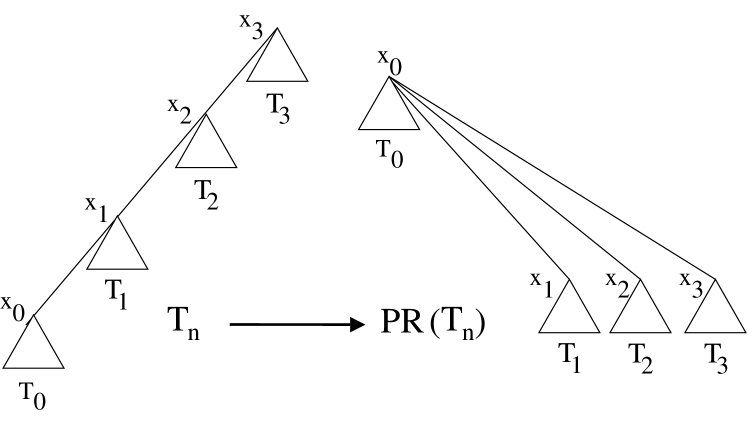
Figure 1: Path reversal $\varphi_{x_{0}}$. The $T_{i}$’s denote the (left/right) subtrees of $T_{n}$.

The average cost of a path reversal performed on an initial ordered $n$-node tree $T_{n}$ which consists of a root with $n-1$ descendants (or children, as in [7]) is the expected number of edges on the paths reversed in $T_{n}$ (see Figure 1). In words, it is the expected height of such reversed trees $\varphi(T_{n})$, provided that we let the height of a tree root be 1: viz. the height of a node $x$ in $T_{n}$ is thus defined as being the number of nodes on the path from the node $x$ to the root $r$ of $T_{n}$.

It turns out that the average number of messages used in $\cal A$ is actually the expected cost of a path reversal performed on such initial ordered $n$-node trees $T_{n}$ which consist of a root with $n-1$ children. This is indeed the average number of changes of the variable Last which builds the dynamic data structure of path reversal used in algorithm $\cal A$.

2.2 Priority queues, tournament trees and permutations

Whenever two combinatorial structures are counted by the same number, there exist one-one mappings between the two structures. Explicit one-to-one correspondences between combinatorial representations provide coding and decoding algorithms between the stuctures. We now need the following definitions of some combinatorial structures which are closely connected with path reversal and involved in the computation of its cost.

2.2.1 Definitions and notations

(i) Let $[n]$ be the set $\{1,2,\ldots,n\}$. A permutation is a one-one mapping $\sigma:[n]\rightarrow[n]$; we write $\sigma\in S_{n}$, where $S_{n}$ is the symmetric group over $[n]$.

(ii) A binary tournament tree of size $n$ is a binary $n$-node tree whose internal nodes are labeled with consecutive integers of $[n]$, in such a way that the root is labeled 1, and all labels are decreasing (bottom-up) along each branch. Let ${\cal T}_{n}$ denote the set of all binary tournament trees of size $n$. ${\cal T}_{n}$ also denotes the set of tournament representations of all permutations $\sigma~{}\in~{}S_{n}$, considered as elements of $[n]^{n}$, since the correspondence $\tau:S_{n}\rightarrow{\cal T}_{n}$ is one-one (see [16] for a detailed proof). Note that this one-to-one mapping implies that $\left|{\cal T}_{n}\right|=n!$

(iii) A priority queue of size $n$ is a set $Q_{n}$ of keys ; each key $K\in Q_{n}$ has an associated priority $p(K)$ which is an arbitrary integer. To avoid cumbersome notations, we identify $Q_{n}$ with the set of priorities of its keys. Strictly speaking, this is a set with repetitions since priorities need not be all distincts. However, it is convenient to ignore this technicality and assume distinct priorities. The simplest representation of a priority queue of size $n$ is then a sequence $s~{}=~{}(p_{1},p_{2},~{}\ldots~{},p_{n})$ of the priorities of $Q_{n}$, kept in their order of arrival. Assume the $n!$ possible orders of arrival of the $p_{i}$’s to be equally likely, a priority queue $Q_{n}$ (i.e. a sequence $s$ of $p_{i}$’s) is defined as random iff it is associated to a random order of the $p_{i}$’s. There is a one-to-one correspondence between the set ${\cal T}_{n}$ of all the $n$-node binary tournament trees and the set of all the priority queues $Q_{n}$ of size $n$. To each one sequence of priorities $s=(p_{1},\ldots,p_{n})\in Q_{n}$, we associate a binary tournament tree $\gamma(s)=T\in{\cal T}_{n}$ by the following rules: let m$\;=\;\min(s)$, we then write $s=\ell\;\mbox{\bf m}\;r$; the binary tree $T\in{\cal T}_{n}$ possesses m as root, $\gamma(\ell)$ as left subtree and $\gamma(r)$ as right subtree. The rules are applied repeatedly to all the left and right subsequences of $s$, and from the root of $T$ to the leaves of $T$; by convention, we let $\gamma(\emptyset)=\Lambda$ (where $\Lambda$ denotes the empty binary tree). The correspondence $\gamma$ is obviously one-one (see [6] for a fully detailed constructive proof).

We shall thus use binary tournaments ${\cal T}_{n}$ to represent the permutations of $S_{n}$ as well as the priority queues $Q_{n}$ of size $n$.

(iv) If $T\in{\cal T}_{n}$ is a binary tournament, its right branch $RB(T)$ is the increasing sequence of priorities found on the path starting at the root of $T$ and repeatedly going to the right subtree. The bottom of $RB(T)$ is the node having no right son. The left branch $LB(T)$ of $T$ is defined in a symmetrical manner.

2.3 The one-one correspondence between $Q_{n}$ and $T_{n}$

We now give a constuctive proof of a one-to-one correspondence mapping the given combinatorial structure of ordered trees $T_{n}$ (as defined in the Introduction) onto the priority queues $Q_{n}$.

Theorem 2.1

There is a one-to-one correspondence between the priority queues of size $n,Q_{n}$, and the ordered $n$-node trees $T_{n}$ which consist of a root with $n-1$ children.

• Proof There are many representations of priority queues $Q_{n}$ ; let us consider the $n$-node binary heap structure, which is very simple and perfectly suitable for the constructive proof.

  • First, a binary heap of size $n$ is an essentially complete binary tree. A binary tree is essentially complete if each of its internal nodes possesses exactly two children, with the possible exception of a unique special node situated on level $(h-1)$ (where $h$ denotes the height of the heap), which may possess only a left child and no right child. Moreover, all the leaves are either on level $h$, or else they are on levels $h$ and $(h-1)$, and no leaf is found on level $(h-1)$ to the left of an internal node at the same level. The unique special node, if it exists, is to the right of all the other level $(h-1)$ internal nodes in the subtree.
    Besides, each tree node in a binary heap contains one item, with the items arranged in heap order (i.e. the priority queue ordering): the key of the item in the parent node is strictly smaller than the key of the item in any descendant’s node. Thus the root is located at position 1 and contains an item of minimum key. If we number the nodes of such a essentially complete binary tree from 1 to $n$ in heap order and identify nodes with numbers, the parent of the node located at position $x$ is located at $\lfloor x/2\rfloor$. Similarly, The left son of node $x$ is located at $2x$ and its right son at $\min\{2x+1,n\}$. We can thus represent each node by an integer and the entire binary heap by a map from $[n]$ onto the items: the binary heap with $n$ nodes fits well into locations $1,\ldots,n$. This forces a breadth-first, left-to-right filling of the binary tree, i.e. a heap or priority queue ordering.

  • Next, it is well-known that any ordered tree with $n$ nodes may easily be transformed into a binary tree by the natural correspondence between ordered trees and binary trees. The corresponding binary tree is obtained by linking together the brothering nodes of the given ordered tree and removing vertical links except from a father to its first (left) son.
    Conversely, it is easy to see that any binary tree may be represented as an ordered tree by reversing the process. The correspondence is thus one-one (see [8, Vol. 1, page 333]).

  Note that the construction of a binary heap of size $n$ can be carried out in a linear time, and more precisely in $\Theta(n)$ sift-up operations.

  Now, to each one sequence of priorities $s=(p_{1},\ldots,p_{n})\in Q_{n}$, we may associate a unique $n$-node tree $\alpha(s)=T_{n}$ in the natural breadth-first, left-to-right order; by convention, we also let $\alpha(\emptyset)=\Lambda$. In such a representation, $T_{n}=\alpha(s)$ is then an ordered $n$-node tree the ordering of which is the priority queue (or heap) order, and it is thus built as an essentially complete binary heap of size $n$. The correspondence $\alpha$ naturally represents the priority queues $Q_{n}$ of size $n$ as ordered trees $T_{n}$ with $n$ nodes.

  Conversely, to any ordered tree $T_{n}$ with $n$ nodes, we may associate a binary tree with heap ordered nodes, that is an essentially complete binary heap. Hence, there exists a correspondence $\beta$ mapping any given ordered $n$-node tree $T_{n}$ onto a unique sequence of priorities $s=\beta(T_{n})\in Q_{n}$; by convention we again let $\beta(\Lambda)=\emptyset$.

  The correspondence is one-one, and it is easily seen that mappings $\alpha$ and $\beta$ are respective inverses. $\Box$

Let binary tournament trees represent each one of the above structures. Any operation can thus be performed as if dealing with ordered trees $T_{n}$, whereas binary tournament trees or permutations are really manipulated. More precisely, since we know that $T_{n}\longleftrightarrow Q_{n}\longleftrightarrow{\cal T}_{n}\longleftrightarrow S_{n}$, the cost of path reversal performed on initial $n$-node trees $T_{n}$ which consist of a root with $n-1$ children is transported from the $T_{n}$’s onto the tournament trees $T\in{\cal T}_{n}$ and onto the permutations $\sigma\in S_{n}$. In the following definitions (see Section 3.1 below), we therefore let $\varphi(\sigma)\in S_{n}$ denote the “reversed” permutation which corresponds to the reversed tree $T_{n}$. From this point the first moment of the cost of path reversal, $\varphi:T_{n}\rightarrow T_{n}$, can be derived, and a straightforward proof technique of the result, distinct from the one in section 3 below, is also detailed in the Appendix.

3 Expected cost of path reversal, average message complexity of $\cal A$

It is fully detailed in the Introduction how the two data structures at hand are actually involved in algorithm $\cal A$ and the design of the algorithm takes place in [12, 15].

3.1 Analysis

Eq. (13) proved in the Appendix, is actually sufficient to provide the average cost of path reversal. However, since we also desire to know the second moment of the cost, we do need the probability generating function of the probabilities $p_{n,k}$, defined as follows.

Let $h(T_{n})$ denote the height of $T_{n}$, i.e. the number of nodes on the path from the deepest node in $T_{n}$ to the root of $T_{n}$, and let $T\in{\cal T}_{n-1}$.

$$p_{n,k}\;=\;\Pr\{\mbox{cost of path reversal for}\ T_{n}\ \mbox{is}\ k\}\;=\;\Pr\{h(\varphi(T))=k\}$$

is the probability that the tournament tree $\varphi(T)$ is of height $k$. We also have

$$p_{n,k}\;=\;\Pr\{k\ \mbox{changes occur in the variable {Last} of algorithm}{\cal A}\}.$$

More precisely, let a swap be any interchanged pair of adjacent prime cycles (see [8, Vol. 3, pages 28-30]) in a permutation $\sigma$ of $[n-1]$ to obtain the “reversed” permutation $\varphi_{x}(\sigma)$ corresponding to the path reversal performed at a node $x\in T_{n}$, that is any interchange which occurs in the relative order of the elements of $\varphi_{x}(\sigma)$ from the one of $\sigma$’s elements, and let $N$ be the number of these swaps occurring from $\sigma\in S_{n-1}$ to $\varphi_{x}(\sigma)$, then,

$$p_{n,k}\>=\;\frac{1}{(n-1)!}\,(\mbox{number of}\ \sigma\in S_{n-1}\ \mbox{for which}\ N=k),$$

since the cost of a path reversal at the root of an ordered tree such as $T_{n}$ is zero.

Lemma 3.1

Let $P_{n}(z)=\sum_{k\geq 0}p_{n,k}z^{k}$ be the probability generating function of the $p_{n,k}$’s. We have the following identity,

$$P_{n}(z)\>=\;\prod_{j=1}^{n-1}\frac{z+j-1}{j}\,.$$

• Proof We have $p_{1,0}=1$ and $p_{1,k}=0$ for all $k>0$.

  A fundamental point in this derivation is that we are averaging not over all tournament trees $T\in{\cal T}_{n-1}$, but over all possible orders of the elements of $S_{n-1}$. Thus, every permutation of $(n-1)$ elements with $k$ swaps corresponds to $(n-2)$ permutations of $(n-2)$ elements with $k$ swaps and one permutation of $(n-2)$ elements with $(k-1)$ swaps. This leads directly to the recurrence

  $$(n-1)!p_{n,k}\;=\;(n-2)(n-2)!\,p_{n-1,k}\;+\;(n-2)!p_{n-1,k-1},$$

  or

  $$p_{n,k}=\;\left(1-\frac{1}{n-1}\right)p_{n-1,k}\;+\;\left(\frac{1}{n-1}\right)p_{n-1,k-1}.$$ (1)

  Consider any permutation $\sigma=\langle\sigma_{1}\ldots\sigma_{n-1}\rangle$ of $[n-1]$. Formula (1) can also be derived directly with the argument that the probability of $N$ being equal to $k$ is the simultaneous occurrence of $\sigma_{i}=j\;\;(1\leq i,j\leq n-1)$ and $N$ being equal to $k-1$ for the remaining elements of $\sigma$, plus the simultaneous occurrence of $\sigma_{i}\neq j\;(1\leq i,j\leq n-1)$ and $N$ being equal to $k$ for the remaining elements of $\sigma$. Therefore,

  $$p_{n,k} = \Pr\{\sigma_{i}=j\}\times p_{n-1,k-1}\;+\;\Pr\{\sigma_{i}\neq j\}\times p_{n-1,k}$$

  $$= \Big{(}1/(n-1)\Big{)}p_{n-1,k-1}\;+\;\Big{(}1-1/(n-1)\Big{)}p_{n-1,k}.$$

  Using now the probability generating function $P_{n}(z)=\>\sum_{k\geq 0}p_{n,k}z^{k}$, we get after multiplying (1) by $z^{k}$ and summing,

  $$(n-1)P_{n}(z)\;=\;zP_{n-1}(z)\;+\;(n-2)P_{n-1}(z),$$

  which yields

  $$P_{n}(z) = \frac{z+n-2}{n-1}\;P_{n-1}(z)$$

  $$P_{1}(z) = z.$$ (2)

  The latter recurrence (2) telescopes immediately to

  $$P_{n}(z)\;=\;\prod_{j=1}^{n-1}\frac{z+j-1}{j}.$$

  $\Box$

• Remark The property proved by Trehel that the average number of messages required by $\cal A$ is exactly the number of nodes at height 2 in the reversed ordered trees $\varphi(T_{n})$ (see [12]) is hidden in the definition of the $p_{n,k}$’s. As a matter of fact, the number of permutations of $[n]$ which contains exactly 2 prime cycles is $\left[\begin{array}[]{c}n\\ 2\end{array}\right]\;=\;(n-1)!\,H_{n-1}$ (see [8]), and whence the result.

Theorem 3.1

The expected cost of path reversal and the average message complexity of algorithm $\cal A$ is $\mbox{$\mathbb{E}$}(C_{n})\>=\;\overline{C_{n}}\>=\>H_{n-1}$, with variance $var(C_{n})\>=\>H_{n-1}\;-\;H_{n-1}^{(2)}$. Asymptotically, for large $n$,

$$\overline{C_{n}}\>=\;\ln n\;+\;\gamma\;+\;O(n^{-1})\ \quad\mbox{and}\ \quad var(C_{n})\;=\;\ln n\;+\;\gamma\;-\;\pi^{2}/6\;+\;O(n^{-1}).$$

• Proof By Lemma 3.1, the probability generating function $P_{n}(z)$ may be regarded as the product of a number of very simple probability generating functions (P.G.F.s), namely, for $1\leq j\leq n-1$,

  $$P_{n}(z)=\;\prod_{1\leq j\leq n-1}\Pi_{j}(z),\ \quad\ \mbox{with}\ \ \Pi_{j}(z)\;=\;\frac{j-1}{j}\;+\;\frac{z}{j}\,.$$

  Therefore, we need only compute moments for the P.G.F. $\Pi_{j}(z)$, and then sum for $j=1$ to $n-1$. This is a classical property of P.G.F.s that one may transform products to sums.

  Now, $\Pi_{j}^{\prime}(1)\;=\;1/j$ and $\Pi_{j}^{\prime\prime}(1)\>=\>0$, and hence

  $$\mbox{$\mathbb{E}$}(C_{n})\;=\>\overline{C_{n}}\>=\;P_{n}^{\prime}(1)\;=\;\sum_{j=1}^{n-1}\Pi_{j}^{\prime}(1)\;=\>H_{n-1}.$$

  Moreover, the variance of $C_{n}$ is

  $$var(C_{n})\>=\;P_{n}^{\prime\prime}(1)\;+\;P_{n}^{\prime}(1)\;-\;P_{n}^{\prime 2}(1),$$

  and thus,

  $$var(C_{n})\>=\;\sum_{j=1}^{n-1}\frac{1}{j}\;-\;\sum_{j=1}^{n-1}\frac{1}{j^{2}}\;=\;H_{n-1}\;-\;H_{n-1}^{(2)}.$$

  Since $H_{n-1}^{(2)}\;=\;\pi^{2}/6\;-\;1/n\>+\>O(n^{-2})$ when $n\rightarrow+\infty$, and by the asymptotic expansion of $H_{n}$, the asymptotic values of $\overline{C_{n}}$ and of $var(C_{n})$ are easily obtained. (Recall that Euler’s constant is $\gamma=0.57721\ldots$, thus $\gamma-\pi^{2}/6\;=\>-1.6772\ldots$)

  Hence, $\overline{C_{n}}=\>.693\ldots\lg n\;+\;O(1)$, and $var(C_{n})=\>.693\ldots\lg n\;+\;O(1)$. $\Box$

Note also that, by a generalization of the central limit theorem to sums of independent but nonidentical random variables, it follows that

$$\frac{C_{n}\>-\>{\overline{C}_{n}}}{(\ln n\,-\,1.06772\ldots)^{1/2}}$$

converges to the normal distribution whe $n\rightarrow+\infty$.

Proposition 3.1

The worst-case message complexity of algorithm $\cal A$ is $O(n)$.

• Proof Let $\Delta$ be the maximum communication delay time in the network and let $\Sigma$ be the minimum delay time for a process to enter, proceed and release the critical section.
  Set $q=\>\left\lceil\Delta/\Sigma\right\rceil$, the number of messages used in $\cal A$ is at most $(n-1)\>+\>(n-1)q\>=\>(n-1)(q+1)\>=O(n)$. $\Box$

Remarks

• The one-to-one correspondence between ordered trees with $(n+1)$ nodes and the words of lenght $2n$ in the Dycklanguage with one type of bracket is used in [12] to compute the average message complexity of $\cal A$. Several properties and results connecting the depth of a Dyckword and the height of the ordered $n$-node trees can be derived from the one-to-one correspondences between combinatorial structures involved in the proof of Theorem 2.1.

• In the first variant of algorithm $\cal A$ (see [15]) which is analysed here, a node never stores more than one request of some other node and hence it only requires $O(\log n)$ bits to store the variables, and the message size is also $O(\log n)$ bits. This is not true of the second variant of algorithm $\cal A$ (designed in [11]). Though the constant factor within the order of magnitude of the average number of messages is claimed to be slightly improved (from 1 downto $.4$), the token now consists of a queue of processes requesting the critical section. Since at most $n-1$ processes belong to the requesting queue, the size of the token is $O(n\log n)$. Therefore, whereas the average message complexity is slightly improved (up to a constant factor), the message size increases from $O(\log n)$ bits to $O(n\log n)$ bits. The bit complexity is thus much larger in the second variant [11] of $\cal A$. Moreover, the state information stored at each node is also $O(n\log n)$ bits in the second variant, which again is much larger than in the first variant of $\cal A$.

4 Waiting time and average waiting time of algorithm $\cal A$

Algorithm $\cal A$ is designed with the notion of token. Recall that a node can enter its critical section only if it has the token. However, unlike the concept of a token circulating continuously in the system, it is sent from one node to another if and only if a request is made for it. The token thus circulates strictly according to the order in which the requests have been made. The queue is updated by each node after executing its own critical section. The queue of requesting processes is maintained at the node containing the token and is transferred along with the token whenever the token is transferred. The requesting nodes receive the token strictly according to the order in the queue.

In order to simplify the analysis, the following is assumed.

• When a node is not in the critical section or is not already in the waiting queue, it generates a request for the token at Poisson rate $\lambda$, i.e. the arrival process is a Poisson process.

• Each node spends a constant time ($\sigma$ time units) in the critical section, i.e. the rate of service is $\mu=1/\sigma$. Suppose we would not assume a constant time spent by each process in the critical section. $\sigma$ could then be regarded as the maximum time spent in the critical section, since any node executes its critical section within a finite time.

• The time for any message to travel from one node to any other node in the complete network is constant and is equal to $\delta$ (communication delay). Since the message delay is finite, we assume here that every message originated at any node is delivered to its destination in a bounded amount of time: in words, the network is assumed to be synchronous

At any instant of time, a node has to be in one of the following two states:

1. Critical state.

   The node is waiting in the queue for the token or is executing its critical section. In this state, it cannot generate any request for the token, and thus the rate of generation of request for entering the critical section by this node is zero.

2. Noncritical state.

   The node is not waiting for the token and is not executing the critical section. In this state, this node generates a request for the token at Poisson rate $\lambda$.

4.1 Waiting time of algorithm $\cal A$

Let ${\cal S}_{k}$ denote the system state when exactly $k$ nodes are in the waiting queue, including the one in the critical section, and let $P_{k}$ denote the probability that the system is in state ${\cal S}_{k}$, $0\leq k\leq n$. In this state, only the remaining $n-k$ nodes can generate a request. Thus, the net rate of request generation in such a situation is $(n-k)\lambda$. Now the service rate is constant at $\mu$ as long as $k$ is positive, i.e. as long as at least one node is there to execute its critical section and the service rate is $0$ when $k=0$. The probability that during the time period $(t,t+h)$ more than one change of state occur at any node is $o(h)$. By using a simple birth-and-death process (see Feller, [4]), the following theorem is obtained.

Theorem 4.1

When there are $k$ $(k>0)$ nodes in the queue, the waiting time of a node for the token is $w_{k}\>=\>(k-1)(\sigma+\delta)\;+\;\sigma/2,$ where $\sigma$ denotes the time to execute the critical section and $\delta$ the communication delay.
The worst-case waiting time is $w_{worst}\>\leq\>(n-1)(\sigma+\delta)\;+\;\sigma/2\;=\>O(n)$.
The exact expected waiting time of the algorithm is

$$\overline{w}\>=\>(\sigma+\delta)(\overline{n}-nP_{n})\;-\;(\delta+\sigma/2)(1-P_{0}-P_{n})\;+\;2\delta P_{0},$$

where $\overline{n}$ denotes the average number of nodes in the queue and the critical section.

• Proof Following equations hold,

  $$P_{0}(t+h) = P_{0}(t)(1-n{\lambda}h)\;+\;P_{1}(t)\Big{(}1\>-\>(n-1){\lambda}h\Big{)}{\mu}h\;+\;o(h)$$

  $$\frac{1}{h}\Big{(}P_{0}(t+h)-P_{0}(t)\Big{)} = -\,n{\lambda}P_{0}(t)\;+\;{\mu}P_{1}(t)\;-\;(n-1){\lambda}{\mu}hP_{1}(t).$$ (3)

  Under steady state equilibrium, $P_{0}^{\prime}(t)=0$ and hence,

  $$\mu P_{1}(t)\;-\;n{\lambda}P_{0}(t)\>=\>0,\;\;\mbox{and}\;P_{1}(t)\;=\;n(\lambda/\mu)P_{0}(t).$$ (4)

  Similarly, for any $k$ such that $1\leq k\leq n$, one can write

  $$P_{k}(t+h) = P_{k}(t)\Big{(}1\>-\>(n-k){\lambda}h\Big{)}(1-{\mu}h)$$

  $$+\ P_{k-1}(t)\Big{(}(n-k+1){\lambda}h\Big{)}(1-{\mu}h)$$

  $$+\ P_{k+1}(t)\Big{(}1\>-\>(n-k-1){\lambda}h\Big{)}({\mu}h)\;+\;o(h),$$

  and

  $$\frac{1}{h}\left(P_{k}(t+h)\>-\>P_{k}(t)\right)\;=\;-(n-k){\lambda}P_{k}(t)\;+\;(n-k+1){\lambda}P_{k-1}(t)\;+\;{\mu}P_{k+1}(t)\;-\;{\mu}P_{k}(t).$$

  Classically, set $\rho=\lambda/\mu$. Proceeding similarly, since under steady state equilibrium $P_{k}^{\prime}(t)=0$,

  $$P_{k+1}(t)\>=\;\left(1+(n-k){\rho}\right)P_{k}(t)\>-\>(n-k+1){\rho},$$ (5)

  and, for any $k$ ($1\leq k\leq n$),

  $$P_{k}(t)\>=\;\frac{n!}{(n-k)!}\>\rho^{k}P_{0}(t)\;=\;n^{\underline{k}}\rho^{k}P_{0}(t).$$ (6)

  For notational brevity, let $P_{k}$ denote $P_{k}(t)$. By Eq. 6, we can now compute the average number of nodes in the queue and the critical section under the form

  $$\overline{n}\>=\>\sum_{k=0}^{n}kP_{k}\>=\>P_{0}\sum_{k=0}^{n}kn^{\underline{k}}\rho^{k},$$

  since the system will always be in one of the $(n+1)$ states ${\cal S}_{0},\ldots,{\cal S}_{n}$, $\sum_{k}P_{k}=1$.

  Now using expressions of $P_{k}$ in terms of $P_{0}$ yields

  $$\sum_{k=0}^{n}P_{k}\;=\;P_{0}\sum_{k=0}^{n}n^{\underline{k}}\rho^{k}\>=\>1.$$

  Thus,

  $$P_{0}\>=\;\left(\sum_{k=0}^{n}n^{\underline{k}}\rho^{k}\right)^{-1}\ \quad\mbox{and}\ \quad P_{i}\>=\;\frac{n^{\underline{i}}\rho^{i}}{\left(\sum_{k=0}^{n}n^{\underline{k}}\rho^{k}\right)}.$$ (7)

  Let there be $k$ nodes in the system when a node $i$ generates a request. Then $(k-1)$ nodes execute their critical section, and one node executes the remaining part of its critical section before $i$ gets the token. Thus, when there are $k$ $(k>0)$ nodes in the queue, the waiting time of a node for the token is

  $w_{k}\>=\>(k-1)$ (time to execute the critical section communication delay $+$

  $+$ average remaining execution time), or

  $$w_{k}\>=\>(k-1)(\sigma+\delta)\;+\;\sigma/2$$ (8)

  (where $\sigma$ denotes the time to execute the critical section and $\delta$ the communication delay).

  When there are zero node in the queue, the waiting time is $w_{0}=2\delta=$ total communication delay of one request and one token message. Hence the expected waiting time is

  $$\mbox{$\mathbb{E}$}(w) = \overline{w}\>=\;\sum_{k=0}^{n-1}w_{k}P_{k}\;=\;2\delta P_{0}\;+\;\sum_{k=1}^{n-1}\left\{(k-1)(\sigma+\delta)\;+\;\frac{\sigma}{2}\right\}P_{k},$$

  $$= (\sigma+\delta)\sum_{k=1}^{n-1}kP_{k}\;-\;(\sigma+\delta)\sum_{k=1}^{n-1}P_{k}\;+\;\sigma/2\sum_{k=1}^{n-1}P_{k}\;+\;2\delta P_{0},$$

  and

  $$\overline{w}\>=\;(\sigma+\delta)(\overline{n}-nP_{n})\;-\;(\delta+\sigma/2)(1-P_{0}-P_{n})\;+\;2\delta P_{0}.$$ (9)

  By Eq. (9), we know the exact value of the expected waiting time of a node for the token in algorithm $\cal A$. Moreover, by Eq. (8), the worst-case waiting time is $w_{worst}\>\leq\;(n-1)(\sigma+\delta)\;+\;\sigma/2\;=\;O(n).$ $\Box$

4.2 Average waiting time of algorithm $\cal A$

The above computation of $\overline{w}$ yields the asymptotic form of an upper bound on the average waiting time $\overline{w}$ of $\cal A$.

Theorem 4.2

If $\rho<1$, the average waiting time of a node for the token in $\cal A$ is asymptotically (when $n\rightarrow+\infty$),

$$\overline{w}\>\leq\>(\sigma+\delta)\left(n(1-2e^{-1/\rho})\right)\;-\;(\delta+\sigma/2)(1-e^{-1/\rho})\;+\;O\left((\sigma/2+3\delta)e^{-1/\rho}\>\frac{\rho^{-n}}{n!}\right).$$

• Proof Assume $\rho=\lambda/\mu<1$, when $n$ is large we can bound $\overline{w}$ from above in Eq. (9) as follows,

  First, $1\>-\>P_{0}\>-\>P_{n}\;=\;1\>-\>P_{0}\>-\>n!\rho^{n}P_{0}$, where $P_{0}=\;\left(\sum_{i=0}^{n}n^{\underline{i}}\rho^{i}\right)^{-1}$.

  Since $\rho<1$,

  $$P_{0}\>\leq\>\left(n!\rho^{n}e^{1/\rho}\right)^{-1},$$

  and, for large $n$,

  $$1\>-\>P_{0}\>-\>P_{n}\;\leq\;1\>-\>\frac{1+n!\rho^{n}}{n!\rho^{n}e^{1/\rho}}\>\leq\>1\;-\;\frac{1}{n!\rho^{n}e^{1/\rho}}\>-\>e^{\textstyle-1/\rho}.$$ (10)

  Next,

  $$P_{n}=\;n!\rho^{n}P_{0}\;\geq\;\frac{\textstyle n!\rho^{n}}{\textstyle n!\rho^{n}e^{1/\rho}}\;=\;e^{\textstyle-1/\rho},$$

  and

  $$\overline{n}\;-\;nP_{n}\;=\;P_{0}\sum_{i=1}^{n}in^{\underline{i}}\rho^{i}\;-\;nP_{n}.$$

  Now,

  $$P_{0}\sum_{i=1}^{n}in^{\underline{i}}\rho^{i} = \frac{\sum_{j=1}^{n}(n-j)\rho^{-j}/j!}{\sum_{j=0}^{n}\rho^{-j}/j!}$$

  $$= n\;-\;\frac{n}{\sum_{j=0}^{n}\rho^{-j}/j!}\;-\;\frac{\sum_{j=1}^{n}j\rho^{-j}/j!}{\sum_{j=0}^{n}\rho^{-j}/j!}$$

  $$\leq n\;-\;\frac{n}{e^{1/\rho}}\;-\;\frac{1}{n!\rho e^{1/\rho}}\,.$$

  Therefore,

  $$\overline{n}\;-\;nP_{n}\;\leq\;n\;-\;ne^{-1/\rho}\;-\;\rho^{-1}e^{-1/\rho}/n!\;-\;ne^{-1/\rho}\;\leq\;n(1\>-\>2e^{-1/\rho})\;-\;\rho^{-1}e^{-1/\rho}/n!$$ (11)

  Thus, by Eqs (9), (10) and (11), we have

  $$\overline{w} \leq (\sigma+\delta)\left(n\left(1\>-\>2e^{-1/\rho}\right)\;-\;\frac{1}{n!\rho e^{1/\rho}}\right)$$

  $$\mbox{}\;-\;(\delta+\sigma/2)\left(1\;-\;\frac{1}{n!\rho^{n}e^{1/\rho}}\;-\;e^{-1/\rho}\right)\;+\;2\delta\left(\sum_{i=0}^{n}n^{\underline{i}}\rho^{i}\right)^{-1},$$

  which yields the desired upper bound for $\rho<1$. When $n$ is large,

  $$\overline{w}\;\leq\;(\sigma+\delta)\left(n(1-2e^{-1/\rho})\right)\;-\;(\delta+\sigma/2)(1-e^{-1/\rho})\;+\;O\left((\sigma/2+3\delta)\>e^{-1/\rho}\frac{\rho^{-n}}{n!}\right).$$

  $\Box$

Corollary 4.1

If $\rho<1$, and irrespective of the values of $\sigma$ and $\delta$, the worst-case waiting time of a node for the token in $\cal A$ is $O(n)$ when $n$ is large.

5 Randomized bounds for the message complexity of $\cal A$ in arbitrary networks

The network considered now is general. The exact cost of a path reversal in a rooted tree $T_{n}$ is therefore much more difficult to compute. The message complexity of the variant $\cal A^{\prime}$ of algorithm $\cal A$ for arbitrary networks is of course modified likewise.

Let $G=(V,E)$ denote the underlying graph of an arbitrary network, and let $d(x,y)$ the distance between two given vertices $x$ and $y$ of $V$. The diameter of the graph $G$ is defined as

$$D\>=\>\max_{x,y\in V}d(x,y).$$

Lemma 5.1

Let $\left|V\right|=n$ be the number of nodes in $G$. The number of messages $M_{n}$ used in the algorithm $\cal A^{\prime}$ for arbitrary networks of size $n$ is such that $0\leq M_{n}\leq 2D$.

• Proof Each request for critical section is at least satisfied by sending zero messages (whenever the request is made by the root), up to at most $2D$ messages, whenever the whole network must be traversed by the request message. $\Box$

In order to bound $D$, we make use of some results of Béla Bollobás about random graphs [2] which yield the following summary results.

Summary results

1. Consider very sparse networks, e.g. for which the underlying graph $G$ is just hardly connected. For almost every such network, the worst-case message complexity of the algorithm is $\Theta(\frac{\log n}{\log\log n})$.

2. For almost every sparse networks (e.g. such that $M=O(n/2)$), the worst-case message complexity of the algorithm is $\Theta(\log n)$.

3. For almost every $r$-regular network, the worst-case message complexity of the algorithm is $O(\log n)$.

6 Conclusion and open problems

The waiting time of algorithm $\cal A$ is of course highly dependent on the values of many system parameters such as the service time $\sigma$ and the communication delay $\delta$. Yet, the performance of $\cal A$, analysed in terms of average and worst-case complexity measures (time and message complexity), is quite comparable with the best existing distributed algorithms for mutual exclusion (e.g. [1, 13]). However, algorithm $\cal A$ is only designed for complete networks and is a priori not fault tolerant, although a fault tolerant version of $\cal A$ could easily be designed. The use of direct one-one correspondences between combinatorial structures and associated probability generating functions proves here a powerful tool to derive the expected and the second moment of the cost of path reversal; such combinatorial and analytic methods are more and more required to complete average-case analyses of distributed algorithms and data structures [5]. From such a point of view, the full analysis of algorithm $\cal A$ completed herein is quite general. Nevertheless, the simulation results obtained in the experimental tests performed in [15] also show a very good agreement with the average-case complexity value computed in the present paper.

Let $\cal C$ be the class of distributed tree-based algorithms for mutual exclusion, em e.g. [1, 13]. There still remain open questions about $\cal A$. In particular, is the algorithm $\cal A$ average-case optimal in the class $\cal C$ ? By the tight upper bound derived in [7], we know that the amortized cost of path reversal is $O(\log n)$. It is therefore likely that the average complexity of $\cal A$ is $\Theta(\log n)$, and whence that algorithm $\cal A$ is average-case optimal in its class $\cal C$. The same argument can be derived from the fact that the average height of $n$-node binary search trees is $\Theta(\log n)$ [5].

Appendix

In Subsection 2.1, we developed the tools which make it possible to derive the first two moments of the cost of path reversal, viz. the expected cost and the variance of the cost (see Subsection 2.2). However, by Theorem 2.1, the average cost of path reversal may be directly proved to be $H_{n-1}$ by solving a straight and simple recurrent equation.

Proposition 6.1

The expected cost of path reversal and the average message complexity of algorithm $\cal A$ evaluate to $\overline{\rm cost}(\varphi(T_{n}))\>=\>\overline{C_{n}}\>=\>H_{n-1}$ (resp.).

• Proof Let $\overline{C_{k}}$ be the average cost of path reversal performed on an initial ordered $k$-node tree $T_{k}$, $1\leq k\leq n$. $\overline{C_{k}}$ is the expected height of $T_{k}$, or the average number of nodes on the path from the node $x$ in $T_{k}$ at which the path reversal is performed to the root of $T_{k}$.

  We thus have $\overline{C_{1}}+1=$ average number of nodes on the path from $x$ to the root in the tree $T_{1}$ with one node ($\overline{C_{1}}+1=1$), $\overline{C_{2}}+1=$ average number of nodes on the path from $x$ to the root in a tree $T_{2}$ with two nodes ($\overline{C_{2}}+1=2$), etc. And therefore, the following identity holds

  $$\overline{C_{k+1}}\>=\;\frac{1}{k}\left((\overline{C_{1}}+1)\>+\>(\overline{C_{2}}+1)\>+\cdots+\>(\overline{C_{k}}+1)\right)\quad\mbox{for}\ k=1,\ldots,n.$$ (12)

  We can rewrite this recurrence in two equivalent forms:

  $$k\overline{C_{k+1}} = k\>+\>\overline{C_{1}}\>+\>\overline{C_{2}}\>+\cdots+\>\overline{C_{k}}\ \qquad(k\geq 1)$$

  $$(k-1)\overline{C_{k}} = (k-1)\>+\>\overline{C_{1}}\>+\>\overline{C_{2}}\>+\cdots+\>\overline{C_{k-1}}\ \qquad(k\geq 2).$$

  Substracting these equations yields

  $$k\overline{C_{k+1}}\>=\>1\>+\>k\overline{C_{k}}\ \ (k\geq 2)\ \quad\mbox{and}\ \ \overline{C_{1}}=0.$$

  Hence,

  $$\overline{C_{k+1}} = \overline{C_{k}}\;+\;1/k,\quad(k\geq 2)$$

  $$\overline{C_{1}} = 0,$$

  and the general formula $\overline{C_{k+1}}\>=\>H_{k}$ follows. Setting $k=n$ finally gives the average cost of path reversal for ordered $n$-node trees,

  $$\overline{C_{n}}\>=\>H_{n-1}.$$ (13)

  $\Box$

Note that if we let $\overline{\left|LB(T)\right|}=\overline{\left|RB(T)\right|}$ denote the mean length of a right or left branch of a tree $T\in{\cal T}_{n-1}$, we also have (by Lemma 2.1)

$$\overline{\rm cost}(\varphi(T_{n}))\>=\>\overline{\left|LB(T)\right|},$$

where $\overline{\left|LB(T)\right|}$ is averaged over all the $(n-1)!$ binary tournament trees in ${\cal T}_{n-1}$.

References

- [1] AGRAWAL D., EL ABBADI A., An Efficient and Fault Tolerant Solution for Distributed Mutual Exclusion, ACM Trans. on Computer Systems, Vol. 9, No 1, 1-20, 1991.
- [2] BOLLOBÁS B., The Evolution of Sparse Graphs, Graph Theory and Combinatorics, 35-57, Academic Press 1984.
- [3] CARVALHO O.S.F., ROUCAIROL G., On Mutual Exclusion in Computer Networks, Comm. of the ACM, Vol. 26, No 2, 145-147, 1983.
- [4] FELLER W., An Introduction to Probability Theory and its Applications, 3rd Edition, Vol. I, Wiley, 1968.
- [5] FLAJOLET P., VITTER J.S., Average-Case Analysis of Algorithms and Data Structures, Res. Rep. INRIA No 718, August 1987.
- [6] FRANÇON J., VIENNOT G., VUILLEMIN J., Description and analysis of an Efficient Priority Queue Representation, Proc. of the 19th Symp. on Foundations of Computer Science, 1-7, 1978.
- [7] GINAT D., SLEATORD. D., TARJAN R.E., A Tight Amortized Bound for Path Reversal, Information Processing Letters Vol. 31, 3-5, 1989.
- [8] KNUTH D.E., The Art of Computer Programming, Vol. 1 & 3, 2nd ed., Addison-Wesley, Reading, MA, 1973.
- [9] LAMPORT L., Time, Clocks and the Ordering of Events in a Distributed System, Comm. of the ACM, Vol. 21, No 7, 558-565, 1978.
- [10] MAEKAWA M., A Algorithm for Mutual Exclusion in Decentralized Systems, ACM Trans. on Computer Systems, Vol. 3, No 2, 145-159, 1985.
- [11] NAÏMI M., TREHEL M., An Improvement of the Distributed Algorithm for the Mutual Exclusion, Proc. of the 7th International Conference On Distributed Computing Systems, 371-375, 1987.
- [12] NAÏMI M., TREHEL M., ARNOLD A., A Distributed Mutual Exclusion Algorithm Based on the Path Reversal, Res. Rep., R.R. du Laboratoire d’Informatique de Besançon, April 1988.
- [13] RAYMOND K., A Tree-Based Algorithm for Distributed Mutual Exclusion, ACM Trans. on Computer Systems, Vol. 7, No 1, 61-77, 1987.
- [14] RICART G., AGRAWALA A.K., An Optimal Algorithm for Mutual Exclusion in Computer Networks, Comm. of the ACM, Vol. 24, No 1, 9-17, 1981.
- [15] TREHEL M., NAÏMI M., A Distributed Algorithm for Mutual Exclusion Based on Data Structures and Fault Tolerance, Proc. of the 6th Annual International Phoenix Conference on Computers and Communications, 35-39, 1987.
- [16] VUILLEMIN J., A Unifying Look at Data Structures, Comm. of the ACM, Vol. 23, No 4, 229-239, 1980.