Lossy Bulk Synchronous Parallel Processing Model for Very Large Scale Grids

Abstract

The performance of a parallel algorithm in a very large scale grid is significantly influenced by the underlying Internet protocols and inter-connectivity. Many grid programming platforms use TCP due to its reliability, usually with some optimizations to reduce its costs. However, TCP does not perform well in a high bandwidth and high delay network environment. On the other hand, UDP is the fastest protocol available because it omits connection setup process, acknowledgments and retransmissions sacrificing reliable transfer. Many new bulk data transfer schemes using UDP for data transmission such as RBUDP, Tsunami, and SABUL have been introduced and shown to have better performance compared to TCP. In this paper, we consider the use of UDP and examine the relationship between packet loss and speedup with respect to the number of grid nodes. Our measurement suggests that packet loss rates between $5\%$-$15\%$ on average are not uncommon between PlanetLab nodes that are widely distributed over the Internet. We show that transmitting multiple copies of same packet produces higher speedup. We show the minimum number of packet duplication required to maximize the possible speedup for a given number of nodes using a BSP based model. Our work demonstrates that by using an appropriate number of packet copies, we can increase performance of parallel program.

I Introduction

Parallel computing has become increasingly popular due to widespread availability of cost effective computational resources, such as commodity SMPs, PCs and high-performance cluster platforms. The size of individual clusters has also continued to grow as evidenced by data collected from the top 500 supercomputers [1]. This has benefited large-scale application research that was once accessible only to a relatively small number of researchers.

However, as the size of computational grids continues to grow, to become very large scale grids (VLSG), the number of wide area network (WAN) connections between islands of clusters and other high performance computing (HPC) centers grows quadratically to the number of nodes. These WAN connections put limits on the granularity of parallel applications that could otherwise benefit from the available computing power, i.e. computation to communication ratio needs to be significantly large in order for the communication complexity to not dominate the run-time. Embarrassingly parallel, data parallel and parametric problems that do not require significant message passing can be efficiently parallelized but problems that require significant communication present challenges. It is important to understand how these problems can be efficiently parallelized. The approach we consider in this paper is to understand the effect of the WAN connections by examining the relationship of network bandwidth, delay, and loss of packets with speedup.

Transmission Control Protocol (TCP) [2] and User Datagram Protocol (UDP) [3] are currently the predominant protocols used for end-to-end communication. TCP provides useful services such as connection-oriented, streaming, full-duplex, reliable, and end-to-end semantic to its applications. These services provide reliability at a cost, causing delay in transmission. Some of these services can be sacrificed depending on the types of applications executed over WAN. Typical grid programming platforms use TCP or TCP with some optimization, but TCP does not perform well in a high bandwidth and high delay network environment [4, 5].

As network bandwidth increases rapidly together with the advent of new routing/switching technology like Multi-protocol Label Switching (MPLS), the load on end systems and the data transfer protocols are becoming bottlenecks in many cases [6]. This indicates performance of parallel programs (mainly constrained by communication phase) on WAN is no longer hardware constrained. Thus we emphasize our study on the bottleneck caused by the data transfer protocol with assumption that end systems with manageable load are used in computing on WAN.

TCPs congestion control algorithm (exponential back-off) causes packet transfer throughput to collapse even when the bandwidth is still plentiful. It is important to realize that packet losses do not necessarily happen just because of network congestion. It is well known that TCP was originally designed for reliable data communication on low bandwidth and high error rate networks [2]. A packet is retransmitted when it gets corrupted or lost. The reliability provided by TCP reduces network throughput, increases average delay and worsens delay jitter [7, 8]. While reliable transmission is quite often critical for the proper execution of a parallel process, use of TCP is not the only means of attaining reliability and it is not clear whether TCP algorithms in general are the correct approach with respect to communication patterns of parallel processes. It is generally accepted that TCP is not suitable for delay constrained applications that emphasize performance issues.

UDP on the other hand tends to be the fastest protocol because it omits connection setup process, acknowledgments, and retransmission. Each packet sent is independent of all other packets. However, unlike TCP, packet losses can occur and a mechanism has to be provided to take necessary measure to detect and assure successful delivery of packets [3].

Many high performance data transfer protocols have been developed using UDP recently. The Tsunami[9] reliable file transfer protocol was developed for high-bandwidth dedicated research networks that never experience significant congestion. It contains two user-space applications (a client and a server) and uses UDP for data transfer and TCP for sending controls information (such as retransmission request, restart request, error report and completion report). This protocol uses inter-packet delay as means of flow control as opposed to sliding-window mechanism in TCP. Another protocol known as Reliable Blast UDP (RBUDP)[10] is an aggressive bulk data transfer scheme. It is intended for extremely high bandwidth, dedicated or Quality-of-Service enabled networks such as optically switched networks. This scheme sends the entire payload at a user-specified sending rate using UDP datagrams and TCP is used to send signal indicating the end of transmission from sender and acknowledgment from receiver consisting bitmap tally of the received packets. This work also demonstrates that the load factor of receiving node contributes to packet loss rate. Simple Available Bandwidth Utilization Library (SABUL) [6] is another high performance data transfer protocol for data intensive application over high bandwidth network. This reliable and lightweight application protocol uses UDP for data transfer and TCP for feedback control messages. It also uses rate based congestion control mechanism that tunes the inter-packet time as in Tsunami. All this work shows that the use of UDP with some reliability can enhance performance for WAN based application that require immense data movements. Thus, we investigate the performance of UDP for parallel computing over WAN.

Our work considers the possibility of achieving good parallel processing speedup using UDP on a WAN with some reliability via acknowledgment packet. We investigate the effect of packet loss on speedup and present a variant of the Bulk Synchronous Parallel (BSP) processing model that considers packet loss as a fundamental parameter. This is because we believe packet loss is the main contributor in performance of UDP based transmission since it is an unreliable protocol. To counter the unreliability of UDP we introduce an acknowledgment packet from the receiver. Thus the packet sending nodes involved in the communication phase knows if a packet is lost (i.e. a packet is not received by a receiving node).

I-A UDP measurements on PlanetLab

To obtain a realistic view of packet loss, bandwidth and round-trip-time on a very large scale grid, we measured UDP behavior for different sizes of packets, between randomly selected nodes from the top level domain ending with “.edu” within PlanetLab [11]. We used utility programs and scripts that we developed to select pairs of nodes randomly from almost $160$ “.edu” nodes. These nodes are then used to measure end to end packet loss, round-trip-time and bandwidth using UDP. $100$ pairs of nodes were used in the experiment and each pairs were run one at a time. Average packet losses between $5\%$-$15\%$ are registered on this platform, plotted in Fig. 1. It is also interesting to note that the percentage of packet loss are independent of packet size for up to $10$ k/bytes, with loss of less than $10\%$ and increases slightly to about $15\%$ for larger packet sizes. There are cases when packet losses exceeds $15\%$, this is probably due to high load and physical links on end systems. Bandwidth and round-trip-time was also measured for UDP on PlanetLab as depicted in Fig. 2 and Fig. 3 respectively. We observed that bandwidth of $30$Mbytes per second to $50$Mbytes per second on average can be achieved using UDP. Round-trip-time between $0.05$s and $0.1$s on average are recorded for packet sizes of up to $25$Kbytes. Using these information we analyzed the best speedup that can be achieved for differing packet loss probability. The extent to which these measurements are indicative of the Internet in general is to be further investigated, though it is reasonable to suggest that a large scale, shared grid system will exhibit similar behavior.

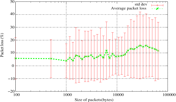
Figure 1: Average packet loss between pairs of nodes for UDP based transmission within PlanetLab.

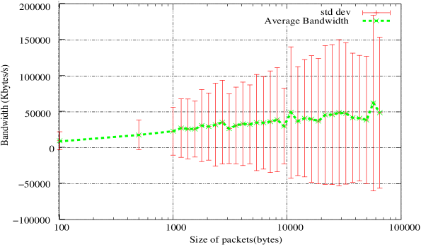
Figure 2: Average bandwidth between pairs of nodes for UDP based transmission within PlanetLab.

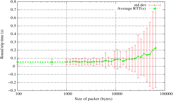
Figure 3: Average round trip time between pairs of nodes for UDP based transmission within PlanetLab.

In section 2, we introduce stochastic models to analyze the impact of packet loss on speedup; section 3 explains how we derived the number of packet copies to use for maximizing the speedup; section 4 analyzes speedup of parallel computation when only lost packets are re-transmitted; section 5 discuss some related work on traditional systems and on WAN systems; and in section 6 we summarize our conclusions and future work.

II The approach

This section introduces a couple of approach used to evaluate performance of parallel algorithms that use UDP protocol for communication purposes. We begin with a conceptual approach and later to a more realistic BSP [12] based model that reflects the effect of packet loss. In our analysis, we used the notion of sending multiple copies of the same packet such that the probability of packet loss approaches zero.

\psfrag{(1-p)}{$(1-p)$}\psfrag{(1-p)^2}{$(1-p)^{2}$}\psfrag{(1-p)p}{$(1-p)p$}\psfrag{p}{$p$}\psfrag{Data sent and received}{Data sent and received}\psfrag{Ack sent and received}{Ack sent and received}\psfrag{Data sent but not received}{Data sent but not received}\psfrag{Ack sent but not received}{Ack sent but not received}\psfrag{Sender}{Sender}\psfrag{Receiver}{Receiver}\psfrag{?}{$?$}\psfrag{Probability of}{Probability of}\psfrag{transmission}{transmission}\psfrag{I}{i)}\psfrag{II}{ii)}\psfrag{III}{iii)}\includegraphics[height=202.35622pt,width=187.90244pt]{pack_loss_scen.eps}

Figure 4: Different packet loss scenario for data packet and acknowledgment packet.

Consider sending a packet of data between $2$ nodes with a fixed loss probability of $p$. We assume probability of data packet loss and acknowledgment packet loss are identical. There are three scenarios that could happen as depicted in Fig. 4: i) The data packet sent by sender is successfully received by the receiving node, and an acknowledgment packet sent by the receiver is successfully received by the sender. This happens with a probability of $(1-p)^{2}$. ii) The data packet sent by sender is successfully received by the receiver but the acknowledgment packet sent by the receiver is lost, with a probability of $(1-p)p$. iii) The data packet sent by the sender is lost, with probability of $p$.

The probability of successful delivery is thus given by $(1-p)^{2}$. Let $c(n)$ be the total number of packets transmitted for a particular communication primitive involving $n$ processors. The probability of successful delivery of $c(n)$ data packets and successfully receiving the acknowledgment packets is $p_{s}(n,p)=(1-p)^{2c(n)}$ and the probability of at least one packet loss is $p_{f}(n,p)=1-p_{s}(n,p)$. Ideally, as $n\longrightarrow\infty$, we have maximum capacity for speedup in computing, however $p_{f}(n,p)\longrightarrow 1$ and thus the system fails to operate. As such, we consider the best $n$ to use for a particular communication complexity of $c(n)$.

\psfrag{w}{$w$}\psfrag{c(n)}{$c(n)$}\psfrag{1}{$1$}\psfrag{2}{$2$}\psfrag{r}{$r$}\includegraphics[height=108.405pt,width=173.44756pt]{simpleCom.eps}

Figure 5: Computation, $w$ and communication, $c(n)$ are performed $r$ rounds.

II-A The conceptual approach

In this section we introduce a simplified conceptual notion that communication between computing nodes are zero (an ideal environment for parallel computing). This approach is similar to that of PRAM model that provided the impetus for the existence of better parallel computing models. Our approach here is not suitable for practical purposes, but will be useful to help understand the theoretical approach. The computation and communication are performed for $r$ rounds, (see Fig. 5). The sending node only knows if a round has failed (i.e. at least one packet is lost in the round). When a round has failed, computation $w$ ($w$ is measured in seconds of work on a processor) is performed again and $c(n)$ packets are retransmitted. Here computation is performed again so as to provide some penalty for the packet losses. The conceptual approach is used to predict the best number of computing nodes to use when communication is assumed to be negligible. Let $T(1)=wr$ represent the time taken to perform computation on a single node, thus $T(n)=\frac{wr}{n}$ is the time taken to perform the same computation on $n$ processors. Since $(1-p_{s}(n,p))^{i}p_{s}(n,p)$ is the probability that $i$ attempts fail and the $(i+1)$-th attempt succeeds, we have:

$$\hat{\rho}=\sum_{i=1}^{\infty}ip_{f}(n,p)^{i-1}p_{s}(n,p)=\frac{1}{p_{s}(n,p)}.$$ (1)

$\hat{\rho}$ gives the expected number of times all the packets are transmitted. Therefore, expected time taken on $n$ processor with packet loss probability $p$, $\hat{T}(n,p)$, is given by  $\hat{T}(n,p)=w\hat{\rho}r=\frac{wr}{np_{s}(n,p)}$ to represent the total time taken to complete the computation on $n$ processors. Hence, expected speedup of $S_{E}=\frac{T(1)}{\hat{T}(n,p)}=np_{s}(n,p)$ can be achieved. Using this expected speedup for different communication $c(n)$, we can determine the optimal number of nodes, $n$, by solving $\frac{\partial{S_{E}}}{\partial{n}}=0$ for $n$.

If $k\geq 2$ copies of the same packets are sent in each round, the probability of success increases and is given by $p^{k}_{s}(n,p)=(1-p^{k})^{2c(n)}$. This approach will require $kc(n)$ packets to be transmitted from the sending nodes and it is better than when $k=1$, with $0<p<1$, and can be shown as below:

$$p \geq p^{k},$$

$$(1-p) \leq(1-p^{k}),$$

$$(1-p)^{2c(n)} \leq(1-p^{k})^{2c(n)},$$

$$p_{s}(n,p) \leq p^{k}_{s}(n,p).$$ (2)

Transmission of $k$ copies of the same packet produces higher probability of transmission success. Techniques used by high performance data transfer protocols mentioned in the previous section can be applied to reduce congestion. Their effect on the model is not considered here. Fig. 7 shows that, when communication is a constant e.g. $c(n)=1$, the speedup increases linearly (note the complexity of speedup $\mathop{\mathrm{O}}\bigl{(}{1}\bigr{)}$, e.g. a single point to point communication in a round), when $c(n)=log_{2}(n)$ (e.g. binomial tree, Bruck and recursive doubling[13] algorithm for broadcast), the speedup is monotonically increasing with $n$, $\mathop{\mathrm{O}}\bigl{(}{n^{(1-2p^{k})}}\bigr{)}$. However, when $c(n)=log_{2}^{2}(n)$, $c(n)=n$ (e.g. Van de Geijin[13] algorithm for broadcast and ring method for all-gather collective communication), $c(n)=nlog_{2}(n)$ and $c(n)=n^{2}$ (e.g. naive all-to-all algorithm) the speedup function is not monotonic and there exists an optimal value of $n$ for a given $p$. The optimal value gives an indication on possible number of nodes $n$ to use when communication cost is zero. Furthermore, it also shows the scalability of an algorithm with different type of communication and varying packet loss probability as depicted in Fig. 7.

\psfrag{Wn}{$\frac{w}{n}$}\psfrag{T1}{$T(1)$}\psfrag{TR}{$T_{R}$}\psfrag{tau}{$2\tau$}\psfrag{1}{$1$}\psfrag{2}{$2$}\psfrag{3}{$3$}\psfrag{R}{$\hat{\rho}$}\includegraphics[height=108.405pt,width=238.49121pt]{bsp_packetloss.eps}

Figure 6: Retransmission of packets using UDP in BSP type parallel program in a superstep.

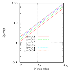
(a) $c(n)=1$

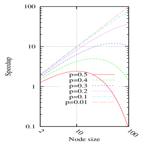
(b) $c(n)=log_{2}(n)$

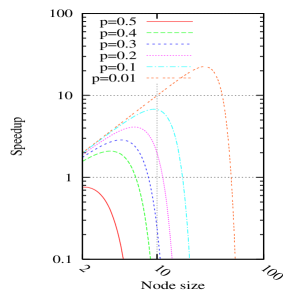
(c) $c(n)=log_{2}^{2}(n)$

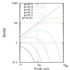
(d) $c(n)=n$

(e) $c(n)=nlog_{2}(n)$

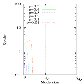
(f) $c(n)=n^{2}$

Figure 7: Graph depicts speedup achieved for communication $c(n)$ at different packet loss probabilities Vs number of processing nodes with $k=2$ for the conceptual approach.

The conceptual approach used in this section can be simplified further by using :

$$e^{x}=\lim_{b\rightarrow\infty}\bigg{(}1+\frac{x}{b}\bigg{)}^{b}.$$

Probability of success $p_{s}^{k}(n,p)=(1-p^{k})^{2c(n)}$, can be approximated as $p_{s}^{k}(n,p)\approx e^{-2p^{k}c(n)}$. When communication is $c(n)=log_{2}(n)$, $c(n)=log_{2}^{2}(n)$, $c(n)=n$, $c(n)=nlog_{2}(n)$, and $c(n)=n^{2}$ the expected speedup can be approximated as $S_{E}=ne^{-2p^{k}c(n)}$ when $p$ is small. There exists an optimal value $n$ for given $p$ when communication $c(n)$ is not $1$ or $log_{2}(n)$. For $c(n)=log_{2}^{2}(n)$, $c(n)=n$, and $c(n)=n^{2}$ optimal number of processors to use is $\big{\lfloor}e^{\frac{\ln^{2}2}{4p^{k}}}\big{\rfloor}$,$\big{\lfloor}\frac{1}{2p^{k}}\big{\rfloor}$ and $\bigg{\lfloor}\frac{1}{2\sqrt{p^{k}}}\bigg{\rfloor}$ respectively. When $c(n)=nlog_{2}(n)$, no analytical solution exists but a numerical solution can be found.

III The Lossy BSP (L-BSP) model

In this section a model to better reflect the behavior of parallel programs on VLSG is introduced. This model, called the Lossy BSP (L-BSP), includes important characteristics of the internet such as average end-to-end round-trip time and average end-to-end bandwidth. We fix value of $2\tau$ as the timeout period for sending data packets to and receiving acknowledgment packets from its destination respectively, refer Fig. 6. $\tau$ is defined as:

$$\tau=\frac{c(n)}{n}\alpha+\beta.$$

where $\alpha=\frac{packet\text{ }size}{bandwidth}$ and $\beta$, the delay is the round trip time (includes cost for sending data and receiving acknowledgment packet). $T(1)=wr$ is the time taken for computation in one processor, with $r$ as the number of times computation is repeated (known as supersteps in BSP model). Whereas, $T_{R}=\frac{w}{n}+2\hat{\rho}\tau$ refers to the expected time that $n$ processors will take to complete a single round as shown in Fig. 6. With zero packet loss (i.e. $\hat{\rho}=1$), time $T(n,\tau)=\frac{T(1)}{n}+2r\tau$ for computation and communication on $n$ nodes can be achieved. Ideally, we expect speedup $S_{I}=\frac{T(1)}{T(n,\tau)}=n$, assuming zero communication cost (i.e. $\tau=0$). However, with an expected average number of transmission $\hat{\rho}=\frac{1}{p_{s}(n,p)}$ (all packets are re-transmitted if a packet is lost), the expected time taken for computation and communication is given by $\hat{T}(n,p,\tau)=\frac{T(1)}{n}+\frac{2r\tau}{p_{s}(n,p)}$. Hence, the expected speedup achievable is:

$$S_{E}=\frac{wr}{\frac{T_{1}}{n}+\frac{2r\tau}{p_{s}(n,p)}}=\frac{w}{\frac{w}{n}+\frac{2\tau}{p_{s}(n,p)}}=\frac{nGp_{s}(n,p)}{1+Gp_{s}(n,p)},$$

where granularity (ratio of computation and communication costs) is $G=\frac{w}{2n\tau}$.

If only lost packets are re-transmitted, data packets that have been successfully sent will not be re-transmitted again. Therefore, the sequence of packet transmission is given by $c(n)$, $pc(n)$, $p^{2}c(n)$, $p^{3}c(n)$,$\cdots$. That is, in the first transmission $c(n)$ packets are sent, in the second transmission only packets that are lost (i.e. $pc(n)$) are re-transmitted and so on. The notion used in ( 1) can also be applied in this model. If $p_{s}=(1-p)^{2}$ is the probability of successful delivery of a single packet and $c(n)$ is the number of packets transmitted then the probability that a communication terminates in the $i$-th re-transmission is $(1-p_{s})^{(i-1)}p_{s}$ for a single packet. Thus, $\sum_{j=1}^{i}(1-p_{s})^{(j-1)}p_{s}$ is the probability that a communication terminates by $i$th re-transmission and $\big{[}\sum_{j=1}^{i}(1-p_{s})^{(j-1)}p_{s}\big{]}^{c(n)}$ is the probability that all communications terminate by $i$-th re-transmission. It follows that, the average number of re-transmission can be obtained from:

$$\hat{\rho}(p_{s},c(n))=\sum_{i=1}^{\infty}i\bigg{(}\bigg{[}\sum_{j=1}^{i}(1-p_{s})^{(j-1)}p_{s}\bigg{]}^{c(n)}-$$

$$\bigg{[}\sum_{j=1}^{i-1}(1-p_{s})^{(j-1)}p_{s}\bigg{]}^{c(n)}\bigg{)}$$

$$=\sum_{i=1}^{\infty}i\bigg{(}\bigg{[}1-(1-p_{s})^{i}\bigg{]}^{c(n)}-\bigg{[}1-(1-p_{s})^{i-1}\bigg{]}^{c(n)}\bigg{)}$$

The value of $\hat{\rho}(p_{s},c(n))$ depends on packet loss $p$ and communication $c(n)$. We use numerical approach to obtain values of $\hat{\rho}(p_{s},c(n))$ for different number of nodes. Thus the expected speedup obtained using the L-BSP model can be simplified as:

$$S_{E}=\frac{Gn}{G+\hat{\rho}{(p_{s},c(n))}}$$ (4)

with granularity, $G=\frac{w}{2n\tau}$. Clearly, speedup approaches linearity when $G\gg\hat{\rho}(p_{s},c(n))$. Fig. 8 shows the effect of granularity for different communication $c(n)$. For higher communication complexity such as $c(n)=nlog_{2}(n)$ and $c(n)=n^{2}$, Fig. 8(e) and Fig. 8(f) respectively, speedup deteriorates at a faster rate.

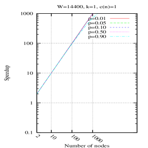
(a) $c(n)=1$

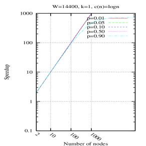
(b) $c(n)=log_{2}(n)$

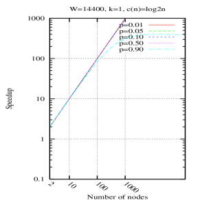
(c) $c(n)=log_{2}^{2}(n)$

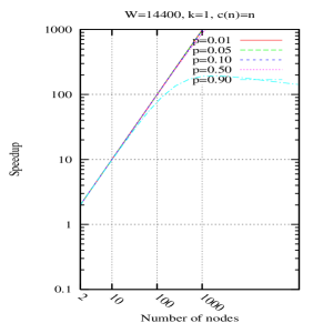
(d) $c(n)=n$

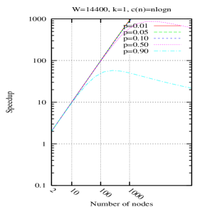
(e) $c(n)=nlog_{2}(n)$

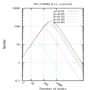
(f) $c(n)=n^{2}$

Figure 8: Graph depicts speedup achieved for different number of nodes $n$, work $W=4$ hours, communication $c(n)$ at different packet loss probability with $k=1$ for the L-BSP model.

Fig. 9 depicts the limits of speedup for different probability of packet losses when different number of nodes are used. It shows that when packet loss is lower, higher speedup can be achieved. Number of optimal nodes to use depend on different operating conditions such as computational and communication complexity. When packet loss is higher, speedup deteriorates at a faster rate. On the other hand, it demonstrates the important effect of granularity on speedup. Linear speedup is possible with higher granularity and correct number of nodes, this is true even for higher degree of communication complexity and packet loss. (e.g. $n=2$)

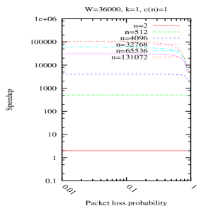
(a) $c(n)=1$

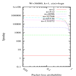
(b) $c(n)=log_{2}(n)$

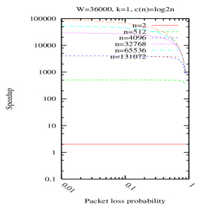
(c) $c(n)=log_{2}^{2}(n)$

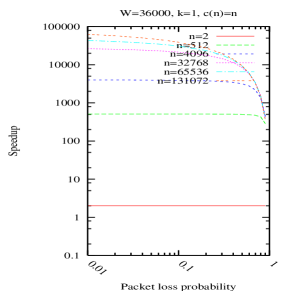
(d) $c(n)=n$

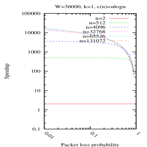
(e) $c(n)=nlog_{2}(n)$

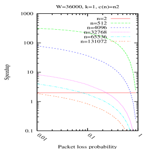
(f) $c(n)=n^{2}$

Figure 9: Graph depicts speedup for different packet loss probabilities given $n$ nodes, work $W=10$ hours, and communication $c(n)$ for the L-BSP model.

IV Optimal packet copies

The conceptual approach revealed that speedup can be increased by transmitting multiple copies of the same packet. It is easy to verify that as $k\rightarrow\infty$, we have $p_{s}\rightarrow 1$, however, it is unrealistic to send that many packet copies. Thus, finding optimal value for $k$ is necessary for a given value of $p$, $n$, $w$ and $c(n)$.

We consider this scenario in the L-BSP model. If $k$ copies of same packets are sent, ( 4), can be re-written as:

$$S_{E}=\frac{nG_{1}}{G_{1}+\hat{\rho}^{k}(p_{s}^{k},c(n))},$$ (5)

with $p_{s}^{k}=(1-p^{k})^{2}$, $\hat{\rho}^{k}(p_{s}^{k},c(n))$ the average number of transmissions when $k$ packet copies are used, and $G_{1}=\frac{w}{2n\tau_{k}}$ where $\tau_{k}$ is defined as $\tau_{k}=k\frac{c(n)}{n}\alpha+\beta$ and $2\tau_{k}$ represents the timeout value for sending $kc(n)$ packets.

Equation ( 5) can be simplified to:

$$S_{E}=\frac{n}{1+\frac{2\hat{\rho}^{k}n}{w}\bigg{(}k\frac{c(n)}{n}\alpha+\beta\bigg{)}}=\frac{n}{1+\frac{2k\hat{\rho}^{k}c(n)\alpha}{w}+\frac{2n\beta\hat{\rho}^{k}}{w}}.$$ (6)

Assuming communication $c(n)=n^{2}$, it is clear that the second term in the denominator,$\frac{2k\hat{\rho}^{k}n^{2}\alpha}{w}$, grows quadratically as $n$ increases in ( 6). Using the numerically solved value for $\hat{\rho}^{k}$ we find the optimal value of $k$, by minimizing the product of $k\hat{\rho}^{k}$. Table. I shows the dominating term that effects the speedup as $n\rightarrow\infty$ for different communication $c(n)$. For lower communication complexity, such as $c(n)=1,log_{2}^{2}(n)$ and $log(n)$, the dominating term as $n$ increases is $\frac{2n\beta\hat{\rho}^{k}}{w}$.

TABLE I: Dominating term for speedup using different type of communications.

Case	Communication $c(n)$	Dominating term as $n\rightarrow\infty$
I	$n^{2}$	$\frac{2k\hat{\rho}^{k}c(n)\alpha}{w}$
II	$nlog_{2}(n)$	$\frac{2k\hat{\rho}^{k}c(n)\alpha}{w}$
III	$n$	$\frac{2k\hat{\rho}^{k}c(n)\alpha}{w}+\frac{2n\beta\hat{\rho}^{k}}{w}$
IV	$log_{2}^{2}(n)$	$\frac{2n\beta\hat{\rho}^{k}}{w}$
V	$log_{2}(n)$	$\frac{2n\beta\hat{\rho}^{k}}{w}$
VI	$1$	$\frac{2n\beta\hat{\rho}^{k}}{w}$

As the time to transmit the packet, $\alpha$, approaches zero (i.e. transmission cost approaches zero) ( 6) can be reduced to:

$$\lim_{\begin{subarray}{c}k\rightarrow\infty\\ \alpha\rightarrow 0\end{subarray}}S_{E}=\frac{n}{\frac{2n\beta}{w}+1}.$$

Here, $\hat{\rho}^{k}\rightarrow 1$, as number of packet copies, $k$, transmitted increases. It indicates that work performed on each node should be large enough compared to the average delay between nodes to achieve good speedup.

Fig. 10 shows how speedup is effected by the number of packet copies transmitted for work of $w=10$ hours. It is clear from the figure that for communication $c(n)=n$, $c(n)=nlog_{2}(n)$ and $c(n)=n^{2}$ speedup deteriorates as the number of packet copies used increases. This observation concurs with the expected decrease in speedup, because of higher overhead caused by more packets and higher communication complexity.

Fig. 11 and Fig. 12 shows predicted speedup with different work loads, for different packet loss probabilities. These graphs are for $n=2$ and $n=131072$ nodes respectively when $k=1$. As the size of work increases on each processor, speedup approaches the total number of processor used for higher granularity.

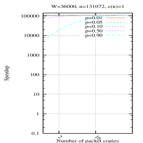
(a) $c(n)=1$

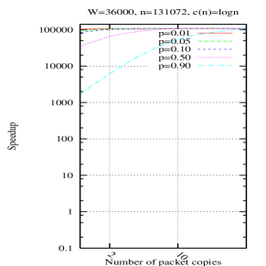
(b) $c(n)=log_{2}(n)$

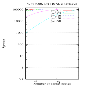
(c) $c(n)=log_{2}^{2}(n)$

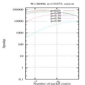
(d) $c(n)=n$

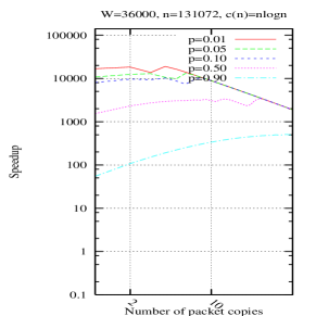
(e) $c(n)=nlog_{2}(n)$

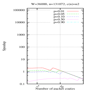
(f) $c(n)=n^{2}$

Figure 10: Graph depicts speedup for different packet copies given $n$ nodes, work $W=10$ hours, communication $c(n)$ at different packet loss probability for the L-BSP model.

(a) $c(n)=1$

(b) $c(n)=log_{2}(n)$

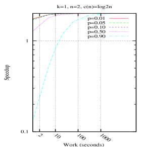
(c) $c(n)=log_{2}^{2}(n)$

(d) $c(n)=n$

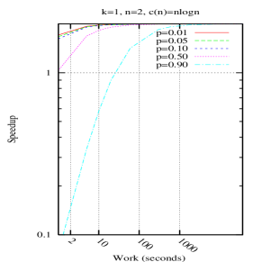
(e) $c(n)=nlog_{2}(n)$

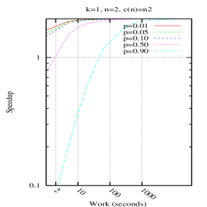
(f) $c(n)=n^{2}$

Figure 11: Graph depicts speedup for different work sizes, for $n=2$, communication $c(n)$ at different packet loss probabilities for the L-BSP model.

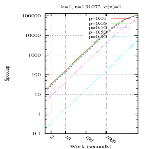
(a) $c(n)=1$

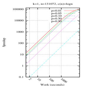
(b) $c(n)=log_{2}(n)$

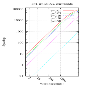
(c) $c(n)=log_{2}^{2}(n)$

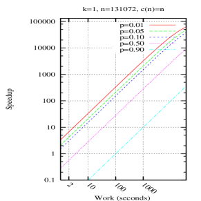
(d) $c(n)=n$

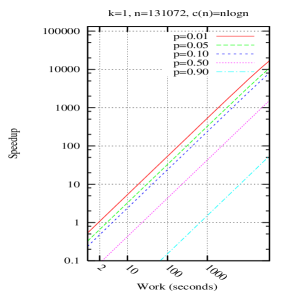
(e) $c(n)=nlog_{2}(n)$

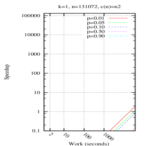
(f) $c(n)=n^{2}$

Figure 12: Graph depicts speedup for different work sizes, for $n=131072$, communication $c(n)$ at different packet loss probabilities for the L-BSP model.

V Adapting fundamental parallel algorithm

In this section, we analyze some fundamental algorithms using the L-BSP model, that provides the number of packet copies, $k$, number of nodes, $n$, amount of work loads, $w$, to use depending on packet loss probability, $p$, and communication complexity, $c(n)$.

The L-BSP model in this paper considers sending data that fits into a single packet. However, the maximum packet size in the Internet Protocol Version 4(IPv4) is only $65$KB, to accommodate large data we can: a) assume the usage of Internet Protocol version 6 (IPv6) that provides maximum packet size of up to $4$GB. b) Use multiple communication supersteps,$\gamma$, where $\gamma=\big{\lceil}\frac{data\text{ }size}{packet\text{ }size}\big{\rceil}$.

Since it was not possible for us to obtain values for packet loss probability, round-trip time and bandwidth using IPv6. This values are extrapolated from our experiment using IPv4 on PlanetLab.

TABLE II: Approximate speedup of parallel algorithms for different parameter values using L-BSP model.

Algorithm	Matrix multiplication,	Bitonic	2D-FFT	Laplace Equation,
	size ($N$x$N$)	Merge sort		size ($N$x$N$)
Size, $N$	$2^{15}$	$2^{31}$	$2^{34}$	$2^{18}$
No. of processors, $n$	$2^{16}$	$2^{17}$	$2^{15}$	$2^{17}$
Size of message (bytes)	$2^{16}$	$2^{16}$	$2^{8}$	$24$
Packet size, $p_{sz}$	$2^{16}$	$2^{16}$	$2^{8}$	$24$
Packet copies, $k$	$7$	$6$	$3$	$5$
Bandwidth,(MBytes/s)	$17.5$	$17.5$	$17.07$	$24$
Packet loss probability, $p$	$0.045$	$0.045$	$0.0005$	$0.0005$
$\frac{p_{sz}}{Bandwidth},\alpha$	$0.0037$	$0.0037$	$0.000015$	$0.000001$
Delay, $\beta$	$0.069$	$0.069$	$0.05$	$0.05$
Average No. of transmission, $\hat{\rho}^{k}$	$1.025$	$1.002$	$1.24$	$1.0$
Sequential compute time (seconds), $w_{s}$	$140765.34$	$133.14$	$5841.15$	$23364.44$
Communication cost (seconds)	$27.54$	$28.18$	$7.35$	$1.7$
Total time in parallel (seconds)	$29.69$	$28.194$	$7.55$	$1.8783$
Communication complexity, $c(n)$	$\mathop{\mathrm{O}}\bigl{(}n^{\frac{3}{2}}\bigr{)}$	$\mathop{\mathrm{O}}\bigl{(}n\bigr{)}$	$\mathop{\mathrm{O}}\bigl{(}n^{2}\bigr{)}$	$\mathop{\mathrm{O}}\bigl{(}n\bigr{)}$
Average processor performance, (GFLOPS)	$0.5$	$0.5$	$0.5$	$0.5$
Speedup, $S_{E}$	$4740.89$	$4.72$	$773.4$	$12439.43$
Efficiency	$0.072$	$0.000036$	$0.02$	$0.095$

V-A Matrix multiplication (Direct implementation)

\psfrag{sqtp}{$\sqrt{P}$}\psfrag{m}{$\frac{N}{\sqrt{P}}$}\psfrag{b}{$A_{1,1}$}\psfrag{c}{$A_{1,2}$}\psfrag{d}{$A_{1,3}$}\psfrag{e}{}\psfrag{f}{$B_{2,4}$}\psfrag{g}{$B_{3,4}$}\psfrag{h}{$B_{4,4}$}\includegraphics[height=144.54pt,width=260.17244pt]{matrix_multip.eps}

Figure 13: Parallel matrix multiplication on $P=16$ nodes.

Consider the product of two matrices $A$ and $B$ of size $N$x$N$, producing matrix $C$ of size $N$x$N$, where $N\in 2^{m}$ and $m\in\mathbb{Z}^{+}$. Each processor, $k$, with $k\in{1,2,\ldots,P}$ where $P$ is the total number of processor, has two submatrices of size $\frac{N}{\sqrt{P}}$x$\frac{N}{\sqrt{P}}$, one from each matrix (i.e. $A$ and $B$) and are indexed as $A_{i,j}$ and $B_{i,j}$, where $i,j\in{1,2,\ldots,\sqrt{P}}$ denote rows and columns respectively. Each submatrix contains $\frac{N^{2}}{P}$ elements. We assume each processor in the system have a submatrix of $A$ and $B$ in them. Squares with same numbers in Fig. 13 denotes submatrix $C_{i,j}$ that can be computed concurrently. During the communication phase, $c(P)=2(P^{\frac{3}{2}}-P)$ packets are injected into the network. At the end of computation each processor has a portion of submatrix $C$ in its possession. On a single processor the cost of computing is $2N^{3}-N^{2}$. Using $P$ processor the cost of sending submatrices from different processor to compute submatrix $C_{i,j}$ as shown in Fig. 13 is $2\gamma\hat{\rho}^{k}(2(\sqrt{P}-1)k\alpha+\beta)$ seconds. The cost of computation is: $2\frac{N^{3}}{P}-\frac{N^{2}}{P}$ FLOPs with the L-BSP model. Thus the expected speedup is:

$$S_{E}=\frac{w_{s}}{w_{p}+2\gamma\hat{\rho}^{k}(2(\sqrt{P}-1)k\alpha+\beta)}$$

with,
$w_{s}=\frac{2N^{3}-N^{2}}{Average\text{ }FLOPS}$ and $w_{p}=\frac{2\frac{N^{3}}{P}-\frac{N^{2}}{P}}{Average\text{ }FLOPS}$.

Using this model, we analyzed achievable speedup for different node sizes $P=2^{s}$ where $s=1,2,3,\ldots,17$ and for different matrix dimensions, $N$x$N$ where $N=2^{11},2^{12},2^{13},2^{14},2^{15}$. A best speedup of $4740.89$ is obtained when $N=2^{15}$ and $P=2^{17}$, Table. II shows the algorithm parameters for this speedup. The analysis shows that matrix multiplication algorithm is very well suited for parallelization on VLSG with our approach. Although the efficiency is low at $0.072$, it is interesting to note that the problem is solvable at almost $4741$ times faster using $2^{15}$ nodes compared to on a single processor.

V-B Sorting (Bitonic mergesort)

Here, we analyze the complexity of Batcher’s bitonic sort algorithm [14]. Assuming each processor in the system has $N$ unsorted keys, rearrange them so that every key in processor $i$ is less than or equal to every key in processor $i+1$ where $1\leq i<P$. First, each processor sorts its $\frac{N}{P}$ keys locally (either ascending or descending order, for obtaining bitonic sequence). Then this algorithm does $log_{2}(P)$ merge stages as shown in Fig. 15, where stage $S$ $(1\leq S\leq log_{2}(P))$ has $S$ merge steps. In merge step $j$ $(1\leq j\leq S)$ of stage $S$, each processor $i$ sends the list of $\frac{N}{P}$ keys in its possession to the processor $x$ ($x$ is obtained by complementing the $j$th bit of $i$). Thereafter, every processor does the merging and keeps either the first half or the second half of the merged list. At the end of sorting, each processor $i$ will have $\frac{N}{P}$ sorted keys that are less or equal to every key in processor $i+1$. [15] A total of $\frac{log_{2}(P)(log_{2}(P)+1)}{2}$ steps are required in this algorithm. In each step, a total of $c(P)=P$, UDP packets are transmitted. The computational cost of sorting an unsorted sequence of size $N$ and merging them in parallel is $\frac{N}{P}log_{2}\big{(}\frac{N}{P}\big{)}+\frac{log_{2}(P)(log_{2}(P)+1)}{2}\big{(}\frac{2N}{P}-1\big{)}$ FLOPs, and the total communication cost is $\gamma(log_{2}(P)(log_{2}(P)+1))(k\alpha+\beta)\hat{\rho}^{k}$ seconds. The expected speedup can be calculated using the L-BSP model as:

$$S_{E}=\frac{w_{s}}{w_{p}+\gamma log_{2}(P)(log_{2}(P)+1)(k\alpha+\beta)\hat{\rho}^{k}}$$

with, $w_{s}=\frac{Nlog_{2}N}{Average\text{ }FLOPS}$ and $w_{p}=\frac{\frac{N}{P}log_{2}\big{(}\frac{N}{P}\big{)}+log_{2}(P)(log_{2}(P)+1)\big{(}\frac{N}{P}-\frac{1}{2}\big{)}}{Average\text{ }FLOPS}$.

\psfrag{1}{$1$}\psfrag{2}{$2$}\psfrag{3}{$3$}\psfrag{4}{$4$}\psfrag{P}{$P$}\psfrag{P-3}{$P-3$}\psfrag{P-2}{$P-2$}\psfrag{P-1}{$P-1$}\psfrag{logp}{$log_{2}(P)$}\psfrag{S=1}{$S=1$}\psfrag{S=2}{$S=2$}\psfrag{S=logp}{$S=log_{2}(P)$}\psfrag{j=1}{$j=1$}\psfrag{j=2}{$j=2$}\psfrag{j=logp-1}{$j=log_{2}(P)-1$}\psfrag{j=logp}{$j=log_{2}(P)$}\psfrag{p-4}{$P-4$}\psfrag{p-3}{$P-3$}\psfrag{p-2}{$P-2$}\psfrag{p-1}{$P-1$}\psfrag{w(w+1)/2}{$\frac{log_{2}(P)(log_{2}(P)+1)}{2}$}\includegraphics[height=144.54pt,width=260.17244pt]{bitonic.eps}

Figure 14: Parallel bitonic mergesort for $P$ nodes.

With this model, achievable speedup for different sizes of data, $N=2^{20},2^{24},2^{28},2^{29},2^{30},2^{31}$ and different number of nodes $P=2^{s}$ where $s=1,2,3,\ldots,17$ were analyzed. The best speedup of $4.722$ was obtained when $P=2^{17}$ and $N=2^{31}$, Table. II shows the algorithm parameters for this speedup. Although, efficiency is very low for this algorithm it is interesting to observe that some speedup can still be obtained on VLSG with our approach.

V-C 2D Fast Fourier Transform (FFT) transpose method (FFT-TM)

Fourier transform plays an important role in many scientific and technical applications. A fast Fourier transform (FFT) has a RAM complexity of $\mathop{\mathrm{O}}\bigl{(}NlogN\bigr{)}$. The FFT can be parallelized using the 2D FFT-TM algorithm. The 2D FFT-TM algorithm can be viewed as computing multiple 1D FFTs in each direction using a fast FFT library (e.g. FFTW) and it has a couple of all-to-all communication for inter-processor data distribution. During this communication, each node will send a portion of its $\frac{N}{P}$ data (i.e. $\frac{N}{P^{2}}$ data) to $P-1$ processors. The received data (complex numbers with datum size of $16$ bytes) is then re-arranged to complete the transpose process. We assume the cost of rearranging the data to be insignificant. In our analysis, all the processor has $\frac{N}{P}$ data in their node initially and only one UDP data packet is required to send $\frac{N}{P^{2}}$ portion of its data to another node. A total of $c(P)=P(P-1)$ UDP data packets of size $\frac{Nb}{P^{2}}$, where $b$ is the data size, are transmitted during the all-to-all data distribution. The total parallel computation cost for this algorithm is given by $10\frac{N}{P}log(\frac{N}{P})$ FLOPs and the communication cost is $4\gamma\hat{\rho}^{k}\big{(}k\alpha(P-1)+\beta\big{)}$ seconds. Following, the expected speedup can be calculated using L-BSP model as:

$$S_{E}=\frac{w_{s}}{w_{p}+4\gamma\hat{\rho}^{k}\big{(}k\alpha(P-1)+\beta\big{)}}$$

with, $w_{s}=\frac{5Nlog(N)}{Average\text{ }FLOPS}$ and $w_{p}=\frac{10\frac{N}{P}log\big{(}\frac{N}{P}\big{)}}{Average\text{ }FLOPS}$.

Using this model, speedup for different node sizes $P=2^{s}$ where $s=1,2,3,\ldots,15$ and for different data sizes, $N$ where $N=2^{30},2^{32},2^{34},2^{36},2^{38}$ were analyzed. A best speedup of $773.4$ with efficiency at $0.02$ is obtained when $N=2^{34}$ and $P=2^{15}$. Table. II shows the algorithm parameters for this speedup. The analysis shows that 2D-FFT algorithm maybe suitable for parallelization on VLSG with our approach for very large data size.

V-D Partial differential equation: The Laplace’s Equation

Partial differential equation is used in many different fields of computational science to model real world phenomena. One of the fundamental partial differential equation is the Laplace’s equation:

$$\frac{\partial^{2}f}{\partial x^{2}}+\frac{\partial^{2}f}{\partial y^{2}}=0,$$

$$f(0,y)=U_{1}(y),f(l,y)=U_{2}(y),$$

$$f(x,0)=U_{3}(x),f(x,l)=U_{4}(x),$$

$$0<x<l,0<y<l.$$

The solution $f(x,y)$, for this equation with given boundary conditions can be found using the finite difference method. First the Laplace equation must be discretized and the resulting system of linear equation is then solved. In matrix-vector form, this system of linear equation has a sparse matrix with $5$ (nonzero elements) diagonals. In this paper, we analyze the Jacobi method used to solve this system. We can represent the function $f(x,y)$ by its values at discrete set of uniformly-spaced network of mesh points, $x_{i}=i\Delta x$ and $y_{j}=j\Delta y$ for $i=0,1,\ldots,m$ and $j=0,1,\ldots,q$ with $\Delta x=\frac{l}{m}$ and $\Delta y=\frac{l}{q}$. The grid size $h$ of $x$-dimension and $y$-dimension are chosen to be equal, $h=\Delta x=\Delta y$ to simplify our analysis. The function $f(x,y)$ at any point $(x_{i},y_{j})$ is represented by $f_{i,j}$. The finite difference representation for Laplace equation is,

$$\frac{f_{i+1,j}-2f_{i,j}+f_{i-1,j}}{h^{2}}+\frac{f_{i,j+1}-2f_{i,j}+f_{i,j-1}}{h^{2}}=0.$$

and can be rearranged as,

$$f^{k+1}_{i,j}=\frac{1}{4}\big{[}f^{k}_{i+1,j}+f^{k}_{i-1,j}+f^{k}_{i,j+1}+f^{k}_{i,j-1}\big{]}.$$

where $f^{k+1}$ is the value obtained from $k+1$th iteration and $f^{k}$ is the value obtained from the $k$th iteration. The $(i,j)$th point is computed from the $ij$th (product of $i$ and $j$) equation. This results in a system of linear equation with $(m-1)^{2}$ equations and $(m-1)^{2}$ unknowns. Jacobi method can be used to solve this equation and is described as:

$$x_{i}^{k}=\frac{1}{a_{i,i}}\big{[}b_{i}-\sum_{j\neq i}a_{i,j}x_{j}^{k-1}\big{]}$$

For a pentadiagonal system with $\frac{(m-1)^{2}}{P}>5$, ($P$ is the number of processors used) each node is required to exchange at most $3$ newly calculated values of unknowns between neighboring nodes. Thus, $c(P)=2(P-1)$ packets of size $3b$ bytes, where $b$, is the data size in bytes, are injected into the network at any one communication. For a diagonally dominant matrix, which is the case for Laplace equation, the Jacobi method will converge to “a good solution” in $log_{2}P$ steps, however this depends on the initial value used and the convergence rate. In our analysis, we take $log_{2}P$ as the number of rounds required for convergence.

The total parallel computation cost for this algorithm is $2dlog_{2}P\big{(}\frac{(m-1)^{2}}{P}\big{)}$ FLOPs, where $d$ is the number of diagonals in the matrix ($d=5$ for a pentadiagonal system). The total communication time is $2log_{2}P\hat{\rho}^{k}\big{(}\alpha k\frac{2(P-1)}{P}+\beta\big{)}$ seconds. Following, the expected speedup can be calculated using L-BSP model as:

$$S_{E}=\frac{w_{s}}{w_{p}+2\hat{\rho}^{k}log_{2}P\big{(}k\alpha\frac{2(P-1)}{P}+\beta\big{)}}$$

with, $w_{s}=\frac{2dlog_{2}P(m-1)^{2}}{Average\text{ }FLOPS}$ and $w_{p}=\frac{2dlog_{2}P\big{(}\frac{(m-1)^{2}}{P}\big{)}}{Average\text{ }FLOPS}$.

\psfrag{m/P}{$\frac{(m-1)^{2}}{P}$}\psfrag{m-1}{${(m-1)}^{2}$}\psfrag{exchg}{Exchange}\includegraphics[height=144.54pt,width=231.26378pt]{Jacobi1.eps}

Figure 15: Each node computes $\frac{(m-1)^{2}}{P}$ points and exchanges at most $3$ newly computed values in a pentadiagonal system.

With this model, achievable speedup for different dimension $m$x$m$, where $m=2^{14},2^{15},2^{16},2^{17},2^{18}$ and different number of nodes $P=2^{s}$ where $s=1,2,3,\ldots,17$ were analyzed. The best speedup of $12439.43$ was obtained when $P=2^{17}$ and $m=2^{18}$, Table. II shows the algorithm parameters for this speedup. Although, efficiency is low at $0.095$ for this algorithm, it is interesting to observe that reasonable speedup can still be obtained on VLSG with our approach.

V-E Broadcast

The broadcast operation is a fundamental primitive in many parallel applications. A broadcast is a communication pattern where a source node sends messages to all other processors in the system. Two commonly used algorithms are the binomial tree for short messages and the one proposed by Van de Geijn [16] for long messages. In the binomial tree algorithm, the root node $P_{0}$ sends data to node $P_{0+\frac{P}{2}}$. These nodes then act as the new roots within their own subtrees and recursively distributes the messages. This communication takes a total of $\lceil logP\rceil$ steps, in the following analysis, we consider messages that fit into a single packet. In step $logP$, $c(P)=logP$ packets are communicated. Thus, the total cost of communication in L-BSP model can be simplified as:

$$t_{bcast}=\bigg{[}\frac{k\alpha}{P}(1-2^{\lceil logP\rceil-1})+\beta\lceil logP\rceil\bigg{]}\hat{\rho}^{k}$$

V-F All-gather

The all-gather is an operation where data from different processors are gathered on all processors. Three different algorithms can be used for this operation: the ring method, recursive doubling and Bruck algorithm. In the ring method each processor $i$ sends its portion of data to processor $i+1$ and receives data from processor $i-1$ (with a wrap around). In the next step, each processor $i$ forwards to processor $i+1$ the data it received from $i-1$ in the previous step. These steps are repeated for $P-1$ times, where $P$ is the number of processor. If $N$ is the total number of data to be gathered on each processor, then at every step each processor sends $\frac{N}{P}$ data from $P-1$ other processors.[13] Here we consider data size that fit into a single packet. Thus, the total cost of communication for ring method in the L-BSP model is, $t_{allgather}=\big{[}k\alpha+\beta\big{]}(P-1)\hat{\rho}^{k}$.

VI Related work

Many computational models have been developed for parallel architecture, each of them try to reflect the behavior of parallel algorithms running on parallel architecture. As stated by Maggs et al [17], models should balance between simplicity with accuracy, abstraction with practicality, and descriptivity with prescriptivity. Early models such as PRAM [18] and its variants that emphasize on PRAMs weakness (e.g. Phase PRAM [19], APRAM [20], LPRAM [21], and BPRAM [22]) have been developed for parallel architectures. Other models such as Postal model [23], BSP [12] and LogP [24] that considers communication costs such as network latency and bandwidth were developed to better reflect behavior of parallel algorithms. Variants of BSP such as D–BSP [25, 26], E–BSP [27] and CGM [28, 29, 30, 31] and models that take memory hierarchy into consideration such as Parallel Hierarchical Memory model (P-HMM) [32], LogP-HMM and LogP-UMH [33] have also been developed. However, there is no single model that has become a standard choice for the parallel computing community. This is due to the heterogeneity in communication topology and architecture. Computational model for grid platform is still at its infancy and not many models have been developed for this platform yet. The two well known computational models for grid are the k-Heterogeneous Bulk Synchronous Parallel (HBSP^k) [34], DynamicBSP [35] and BSPGRID [36]. Although some of these models do consider communication and network latency, they, however, do not consider packet loss as a fundamental parameter in their models. This could be because most of these models assume the usage of TCP protocol for internode communication purposes and other factors in TCP that far outweighs the impact of packet losses. In our approach, we used UDP as the communication protocol. It is well known that packet loss and congestion control mechanism (such as rate based congestion control) are the main contributor to UDPs performance. In this paper we concentrate our attention on the impact of packet loss on performance and the usage of multiple packet copies to improve performance.

VII Conclusion

Providing an accurate model to reflect the behavior of sequential program running on a single computer is difficult due to current technologies in computer architecture. On grids, it becomes even harder as there are many more factors that influence the behavior of computing resources and network.

Experiments that run parallel programs on PlanetLab indicates that the communication phase between nodes on a WAN is the main bottleneck effecting performance of parallel programs, even when computing resources are not highly loaded by other jobs. Thus, it is very necessary to utilize the fastest available protocol (UDP) to execute parallel programs on grids. The weakness of UDP can be remedied by using a light-weight mechanism for reliability to enhance achievable speedup.

In this paper, a new model based on the BSP model that considers packet loss probability as a fundamental parameter is introduced. We measured average packet loss, round trip time, and bandwidth for UDP between pairs of nodes within PlanetLab to better understand the dynamics of WAN. This information is then used in our model to derive the optimal number of packet copies to use in order to maximize the speedup of parallel programs. The effect of packet loss on performance of parallel programs is shown.

We also analyzed a few fundamental algorithms using the L-BSP model. Although the efficiency is very low in some cases, the result shows that it is possible to obtain some speedup when large number of nodes are used. It is also important to note that the result do not incorporate the effect of memory hierarchy.

In future work, other features such as replication of parallel program for fault tolerance and reliability are being considered. We intend to evaluate the performance of parallel program based on L-BSP model and detailed packet loss model [37] for TCP.

References

- [1] A. Bouteiller, P. Lemarinier, G. Krawezik, and F. Cappello, “Coordinated checkpoint versus message log for fault tolerant MPI,” in Cluster 2003, 2003.
- [2] J. Postel, “RFC 793:Transmission Control Protocol,” September 1981.
- [3] ——, “RFC 768:User Datagram Protocol,” August 1980.
- [4] B. Irwin and M. Mathis, “Web100: Facilitating High-Performance Network Use. White Paper for the Internet2 End-to-End Performance Initiative.”
- [5] V. Jacobson, R. Braden, and D. Borman, “RFC 1323:TCP Extensions for High Performance ,” May 1992.
- [6] Y. Gu and R. Grossman, “SABUL: A Transport Protocol for Grid Computing,” Journal of Grid Computing, vol. 1, no. 4, pp. 377–386, 2004.
- [7] W. Feng and P. Tinnakornsrisuphap, “The failure of TCP in high-performance computational grids,” in Supercomputing ’00: Proceedings of the 2000 ACM/IEEE conference on Supercomputing (CDROM). Washington, DC, USA: IEEE Computer Society, 2000.
- [8] P. Liu, M. Meng, Y. Xiufen, and J. Gu, “An UDP-based protocol for Internet robots,” Proceedings of the 4th World Congress on Intelligent Control and Automation, vol. 1, pp. 59–65, 2002.
- [9] M. Meiss, “Tsunami: A High-Speed Rate-Controlled Protocol for File Transfer,” http://steinbeck.ucs.indiana.edu/ mmeiss/papers/tsunami.pdf.
- [10] E. He, J. Leigh, O. Yu, and T. A. Defanti, “Reliable Blast UDP: predictable high perfromance bulk data transfer,” in IEEE Cluster Computing. IEEE Computer Society, 2002, pp. 317–324.
- [11] PlanetLab, “http://www.planet-lab.org/.”
- [12] L. Valiant, “A bridging model for parallel computation,” Communication of the ACM, vol. 33, pp. 103–111, Aug 1990.
- [13] R. Thakur, R. Rabenseifner, and W. Gropp, “Optimization of Collective Operations in MPICH,” International Journal of High Performance Computing, vol. 19, pp. 49–66, 2005.
- [14] K. Batcher, “Sorting Networks and their applications.” in Proceedings of the AFIPS Spring Joint Computing Computers, 1968, pp. 307–314.
- [15] H. A. G. Juurlink, B. H. H.and Wijshoff, “A quantitative comparison of parallel computation models,” ACM Trans. Comput. Syst., vol. 16, no. 3, pp. 271–318, 1998.
- [16] M. Shro and R. Geijn, “Collmark mpi collective communication benchmark,” The University of Texas at Austin,” Technical report, December 1999.
- [17] B. Maggs, L. Matheson, and R. Tarjan, “Models of parallel computation: A survey and synthesis,” in Proc. 28th Hawaii Int. Conf. on System Sciences (HICSS). IEEE, Jan 1995, pp. 61–70.
- [18] S. Fortune and J. Wyllie, “Parallelism in random access machines,” in STOC ’78: Proceedings of the tenth annual ACM symposium on Theory of computing. New York, NY, USA: ACM Press, 1978, pp. 114–118.
- [19] P. B. Gibbons, “A more practical PRAM model,” in SPAA ’89: Proceedings of the first annual ACM symposium on Parallel algorithms and architectures. New York, NY, USA: ACM Press, 1989, pp. 158–168.
- [20] R. Cole and O. Zajicek, “The APRAM: incorporating asynchrony into the PRAM model,” in SPAA ’89: Proceedings of the first annual ACM symposium on Parallel algorithms and architectures. New York, NY, USA: ACM Press, 1989, pp. 169–178.
- [21] A. Aggarwal, A. Chandra, and M. Snir, “Communication complexity of PRAMs,” Theor. Comput. Sci., vol. 71, no. 1, pp. 3–28, 1990.
- [22] A. Aggarwal, A. K. Chandra, and M. Snir, “On communication latency in PRAM computations,” in SPAA ’89: Proceedings of the first annual ACM symposium on Parallel algorithms and architectures. New York, NY, USA: ACM Press, 1989, pp. 11–21.
- [23] A. Bar-Noy and S. Kipnis, “Designing broadcasting algorithms in the postal model for message-passing systems,” in SPAA ’92: Proceedings of the fourth annual ACM symposium on Parallel algorithms and architectures. New York, NY, USA: ACM Press, 1992, pp. 13–22.
- [24] D. Culler, R. Karp, D. Patterson, A. Sahay, K. Schauser, E. Santos, R. Subramonian, and T. Eicken, “LogP: towards a realistic model of parallel computation,” in PPOPP ’93: Proceedings of the fourth ACM SIGPLAN symposium on Principles and practice of parallel programming. New York, NY, USA: ACM Press, 1993, pp. 1–12.
- [25] G. Bilardi, C. Fantozzi, A. Pietracaprina, and G. Pucci, “On the Effectiveness of D–BSP as a Bridging Model of Parallel Computation,” in ICCS ’01: Proceedings of the International Conference on Computational Science-Part II. London, UK: Springer-Verlag, 2001, pp. 579–588.
- [26] P. Torre and C. Kruskal, “Submachine locality in the bulk synchronous setting.(Extended Abstract),” in Euro-Par ’96: Proceedings of the Second International Euro-Par Conference on Parallel Processing-Volume II, vol. 1124. London, UK: Springer-Verlag, August 1996, pp. 352–358.
- [27] B. Juurlink and H. Wijshoff, “The E-BSP Model: Incorporating Unbalanced Communication and General Locality into the BSP Model,” In Proc. Euro-Par’96, vol. 1124, pp. 339–347, January 1996.
- [28] F. Dehne, A. Fabri, and A. Rau-Chaplin, “Scalable Parallel Geometric Algorithms for Coarse Grained Multicomputers,” In Proc. ACM 9th Annual Computational Geometry, pp. 298–307, 1993.
- [29] F. Dehne, C. Kenyon, and A. Fabri, “Scalable Architecture Independent Parallel Geometric Algorithms with HIgh Probability Optimal Times,” In Proc. 6th IEEE Symposium on Parallel and Distributed Processing, pp. 586–593, Oct 1994.
- [30] F. Dehne, X. Deng, P. Dymond, A. Fabri, and A. Kokhar, “A randomized parallel 3D convex hull algorithm for coarse grained multicomputers,” in SPAA ’95: Proceedings of the seventh annual ACM symposium on Parallel algorithms and architectures. New York, NY, USA: ACM Press, 1995, pp. 27–33.
- [31] F. Dehne, “Coarse grained parallel algorithms,” Special issue of Algorithmica, vol. 24, no. 3/4, pp. 173–426, 1999.
- [32] B. H. H. Juurlink and H. A. G. Wijshoff, “The Parallel Hierarchical Memory Model,” in SWAT ’94: Proceedings of the 4th Scandinavian Workshop on Algorithm Theory. London, UK: Springer-Verlag, 1994, pp. 240–251.
- [33] Z. Li and J. H. Mills, P. H.and Reif, “Models and Resource Metrics for Parallel and Distributed Computation,” in Proceedings of the Twenty-Eighth Annual Hawaii International Conference on System Sciences, Hawaii, 1995, pp. 51–60. [Online]. Available: citeseer.ist.psu.edu/li89models.html
- [34] T. Williams, “A General-Purpose Model for Heterogeneous Computation, Ph.D. Thesis.” 2000. [Online]. Available: citeseer.ist.psu.edu/williams00generalpurpose.html
- [35] J. Martin and A. Tiskin, “Dynamic BSP: Towards a Flexible Approach to Parallel Computing over the Grid,” in Communicating Process Architectures, I. East, J. Martin, and P. Welch, Eds. IOS Press, 2004, pp. 219–226.
- [36] V. Vasilev, “BSPGRID: Variable Resources Parallel Computation and Multiprogrammed Parallelism.” Parallel Processing Letters, vol. 13, no. 3, pp. 329–340, 2003.
- [37] J. Padhye, V. Firoui, D. Towsley, and J. Kurose, “Modeling TCP throughput: a simple model and its empirical validation,” in SIGCOMM ’98: Proceedings of the ACM SIGCOMM ’98 conference on Applications, technologies, architectures, and protocols for computer communication. New York, NY, USA: ACM Press, 1998, pp. 303–314.